Nonminimal coupling and inflationary attractors

Inflation not only solves the flatness, horizon, and monopole problems in the standard big bang cosmology, but also provides the initial condition for the formation of the large-scale structure [1, 2, 3, 4]. The quantum fluctuations of the inflaton lead to metric perturbations and imprint the anisotropy signatures in the cosmic microwave background radiation. The Planck measurements of the cosmic microwave background anisotropies give $n_{s}=0.968\pm 0.006$ and $r_{0.002}<0.11$ (95% C.L.) [5, 6]. The central value of $n_{s}$ suggests the relation $n_{s}=1-2/N$ with $N=60$, where $N$ is the number of $e$-folds before the end of inflation. Based on this observation, various parametrizations with $N$ for $n_{s}$, the inflaton $\phi$, the slow roll parameters $\epsilon$ and $\eta$ were proposed to study the property of inflationary models [7, 8, 9, 10, 11, 12, 13, 14, 15]. The parametrizations of $\epsilon(N)$, $\eta(N)$, $n_{s}(N)$ or $\phi(N)$ can be compared with the observational data directly and used to reconstruct the inflationary potentials in the slow roll regime [15].

Many inflationary models have the universal result $n_{s}=1-2/N$ to the leading order approximation in $1/N$ for large $N$. In the Einstein frame, the $R^{2}$ inflation [1] has the effective potential $V(\phi)=V_{0}[1-\exp(-\sqrt{2/3}\,\phi)]^{2}$, so the $R^{2}$ inflation has the scalar tilt $n_{s}=1-2/N$ and the tensor to scalar ratio $r=12/N^{2}$. For the Higgs inflation with the nonminimal coupling $\xi\phi^{2}R$, the same results were obtained in the strong coupling limit $\xi\gg 1$ [16, 17]. Although the results can be obtained for the coupling constant as small as $\xi>0.1$ [16], and the derived $n_{s}$ and $r$ are consistent with the Planck observations even when $\xi>0.003$ [18, 19], the amplitude of the scalar perturbation $A_{s}=2.2\times 10^{-9}$ [6] requires that $\xi\approx 49000\sqrt{\lambda}$ [17]; therefore, the strong coupling limit $\xi\gg 1$ is needed to satisfy the observational constraints. The universal attractor for $R^{2}$ inflation and the Higgs inflation was also derived from more general nonminimal coupling $\xi f(\phi)R$ with the potential $\lambda^{2}f^{2}(\phi)$ for arbitrary function $f(\phi)$ in the strong coupling limit [20]. For the conformal coupling $\xi\phi^{2}R$ with $\xi=-1/6$, the kinetic term for the scalar field $\phi$ in the Einstein frame becomes $\partial\phi^{2}/(1-\phi^{2}/6)^{2}$ and has poles. In terms of the canonical scalar field $\varphi=\sqrt{6}\tanh^{-1}(\phi/\sqrt{6})$, the potential becomes much flatter, which can be used to discuss non-slow-roll dynamics in the original Jordan frame [21]. If we take the monomial potential $V(\phi)$, then we get the T model $V(\varphi)=V_{0}\tanh^{2n}(\varphi/\sqrt{6})$ in the Einstein frame and the universal attractor was also obtained [22, 23]. The universal attractor was generalized to the $\alpha$ attractors with the same $n_{s}$ and $r=12\alpha/N^{2}$ by varying the Kähler curvature [24], in which the kinetic term was generalized to $\partial\phi^{2}/(1-\phi^{2}/6\alpha)^{2}$ and the relation between $\phi$ and the canonical field $\varphi$ becomes $\phi=\sqrt{6\alpha}\tanh(\varphi/\sqrt{6\alpha})$ [25]. Inflation due to the existence of the poles in the kinetic term was discussed in more detail as the generalized pole inflation [26]. Furthermore, these attractors can be described by a general scalar-tensor theory of gravity [27].

In this paper, we show that in the strong coupling limit, any attractor is possible for the nonminimal coupling with an arbitrary coupling function $f(\phi)$. We also discuss how long the coupling constant $\xi$ takes to reach the attractors and the constraint on the energy scale of the model from $A_{s}$. The paper is organized as follows. In Sec. 2, we discuss the derivation of various attractors. The detailed behavior of the $\xi$ attractors are discussed in Sec. 3. The conclusions are drawn in Sec. 4.

As discussed in the previous section, under the limit (20), we can get any attractor behavior associated with the arbitrary potential $U(\psi)$ if we assume $V_{J}(\phi)$ takes the form defined in Eq. (22). To get the E-model attractor with the potential [23, 29],

we take

The spectral index $n_{s}$ and the tensor to scalar ratio $r$ are

where

for $n>1$ and $n/{3(2n-1)}<\alpha<{4n^{2}}/{3(n-1)^{2}}$, or $1/3<n<1$ and $\alpha>{4n^{2}}/{3(3n-1)^{2}}$;

for $n>1$ and $\alpha>{4n^{2}}/{3(n-1)^{2}}$;

for other cases; $u=\sqrt{6\alpha n^{2}+n^{2}-3\alpha n}$, $v=\sqrt{n(3\alpha-6\alpha n+n)}\,$ and $W_{-1}$ is the lower branch of the Lambert $W$ function. When $\alpha\ll 1$, Eq. (41) can be approximated as

so $n_{s}$ and $r$ become [29]

The deviation from the above attractor for $\alpha\sim 1$ is bigger if $n\sim 1$ is smaller.

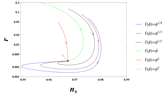
To show that the attractors (37) and (38) can be reached for an arbitrary conformal factor $\Omega(\phi)=1+\xi f(\phi)$, as an example, we take $\omega(\phi)=1$, $n=2$, $\alpha=1$, and the power-law functions $f(\phi)=\phi^{k}$ with $k=1/4$, 1/3, 1/2, 1, 2, and 3. We vary the coupling constant $\xi$ and choose $N=60$ to calculate $n_{s}$ and $r$ for the models with the potential (36), the results are shown in Fig. 1. From Fig. 1, we see that the E-model attractor is reached when $\xi\gtrsim 100$. From Eqs. (37), (38), and (39), we get the attractors $n_{s}=0.9673$ and $r=0.0031$ for $N=60$. The amplitude of the scalar perturbation

Applying the observational result $A_{s}=2.2\times 10^{-9}$ [6], we get the energy scale $V_{0}$ for the E model $V_{0}=4.35\times 10^{-13}$.

To get the T-model attractor with the potential [22, 23],

we take

The spectral index $n_{s}$ and the tensor to scalar ratio $r$ are [24]

for $n>1$ and $(4n^{2}-2n\sqrt{4n^{2}-1})/3<\alpha<{4n^{2}}/{3(n^{2}-1)}$, $1/\sqrt{3}<n<1$ and $\alpha>(4n^{2}-2n\sqrt{4n^{2}-1})/3$ or $1/3<n<1/\sqrt{3}$ and $\alpha>4n^{2}/3(9n^{2}-1)$;

for $n>1$ and $\alpha>{4n^{2}}/{3(n^{2}-1)}$;

for other cases. If $\alpha\ll 1$, Eqs. (52) and (53) become $n_{s}=1-2/N+{2}/{(N^{2}+N)}$ and $r={12\alpha}/{(1+N)^{2}}$.

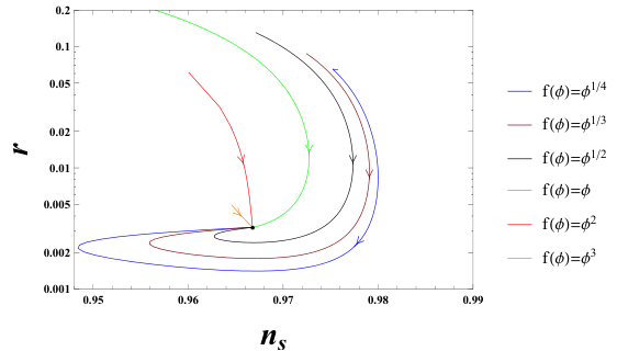
To calculate $n_{s}$ and $r$ explicitly for the potential (47), we take $\omega(\phi)=1$, $n=2$, $\alpha=1$, and the power-law functions $f(\phi)=\phi^{k}$ with $k=1/4$, 1/3, 1/2, 1, 2, and 3. We choose $N=60$ and vary the coupling constant $\xi$; the results are shown in Fig. 2. From Eqs. (48) and (49), we get the attractors $n_{s}=0.9668$ and $r=0.0032$. From Fig. 2, we find that the T-model attractor is reached when $\xi\gtrsim 100$. Using the observational constraint on $A_{s}$ [6], we get the energy scale of the potential $V_{0}=4.55\times 10^{-13}$.

To get the hilltop attractor with the potential,

we take

Here we consider the cases of $n>2$ and $\mu<1$ only. The spectral index $n_{s}$ and the tensor to scalar ratio $r$ are

where

In the large $N$ limit, Eqs. (56) and (57) become [30]

For the potential (55), we choose $\omega(\phi)=1$ and the power-law functions $f(\phi)=\phi^{k}$ with $k=1/3$, 1/2, 2/3, 1, 2 and 3. We calculate $n_{s}$ and $r$ for the cases $n=12$ and $\mu=1/3$, and $N$ is taken to be $N=60$. We show the dependence of $n_{s}$ and $r$ on the coupling constant $\xi$ in Fig. 3 and the results for $n_{s}$ and $r$ in Fig. 4. From Eqs. (56) and (57), we get the Hilltop attractor $n_{s}=0.9640$ and $r=2.6\times 10^{-7}$. The observational constraint on $A_{s}$ gives the energy scale of the potential $V_{0}=3.56\times 10^{-17}$. Figures 3 and 4 tell us that the attractor is reached if $\xi\gtrsim 1$ for $k\leq 1$. For the model with $f(\phi)=\phi^{3}$, we obtain the attractor if $\xi\gtrsim 10^{3}$.

To compare the results with the observations, we replot the $n_{s}$-$r$ graph for the three models along with the observational constraints from Planck 2015 data [6] in Fig. 5, we show the attractors for the coupling functions $f(\phi)=\phi$ and $f(\phi)=\phi^{2}$ only for simplicity. We see that all the three models are consistent with the observational results.

The T model, E model, and the general potential (16) all give the $\alpha$ attractors, and these models can be constructed in supergravity. The universal behaviors are due to the hyperbolic geometry of the moduli space and the flatness of the Kähler potential in the inflaton direction [29]. Under the conformal transformation, the potentials in the Jordan and Einstein frames have the relationship $U(\psi)=V_{J}(\phi)/\Omega^{2}(\phi)$. For any conformal factor $\Omega(\phi)$, we can always choose the corresponding potential $V_{J}(\phi)$ in the Jordan frame so that we have the same potential $U(\psi)$ in the Einstein frame. Therefore, those $\Omega(\phi)$ and $V_{J}(\phi)$ give the same $\xi$ attractor. Furthermore, the attractor can be obtained from $f(R)$ theory. By this method, we may get any attractor we want. In particular, we show explicitly how the T-model, E-model and Hilltop inflations are obtained for an arbitrary conformal factor $\Omega(\phi)$ in the strong coupling limit. These results further support that different models give the same observables $n_{s}$ and $r$, so the existence of $\xi$ attractors imposes a challenge to distinguish different models.

References

• [1] A. A. Starobinsky, Phys. Lett. B. 91, 99 (1980).
• [2] A. H. Guth, Phys. Rev. D 23, 347 (1981).
• [3] A. D. Linde, Phys. Lett. B 129, 177 (1983).
• [4] A. Albrecht and P. J. Steinhardt, Phys. Rev. Lett. 48, 1220 (1982).
• [5] R. Adam et al. (Planck Collaboration), Astron. Astrophys. 594, A1 (2016).
• [6] P.A.R. Ade et al. (Planck Collaboration), Astron. Astrophys. 594, A20 (2016).
• [7] V. Mukhanov, Eur. Phys. J. C 73, 2486 (2013).
• [8] D. Roest, J. Cosmol. Astropart. Phys. 01 (2014) 007.
• [9] J. Garcia-Bellido and D. Roest, Phys. Rev. D 89, 103527 (2014).
• [10] L. Barranco, L. Boubekeur, and O. Mena, Phys. Rev. D 90, 063007 (2014).
• [11] L. Boubekeur, E. Giusarma, O. Mena, and H. Ramírez, Phys. Rev. D 91, 083006 (2015).
• [12] T. Chiba, Prog. Theor. Exp. Phys. 2015, 073E02 (2015).
• [13] P. Creminelli et al., Phys. Rev. D 92, 123528 (2015).
• [14] R. Gobbetti, E. Pajer, and D. Roest, J. Cosmol. Astropart. Phys. 09(2015) 058.
• [15] J. Lin, Q. Gao, and Y. Gong, Mon. Not. R. Astron. Soc. 459, 4029 (2016).
• [16] D. I. Kaiser, Phys. Rev. D 52, 4295 (1995).
• [17] F. L. Bezrukov and M. Shaposhnikov, Phys. Lett. B 659, 703 (2008).
• [18] F. L. Bezrukov and D. Gorbunov, J. High Energy Phys. 07 (2013) 140.
• [19] L. Boubekeur, E. Giusarma, O. Mena, and H. Ramírez, Phys. Rev. D 91, 103004 (2015).
• [20] R. Kallosh, A. Linde, and D. Roest, Phys. Rev. Lett. 112, 011303 (2014).
• [21] K. S. Kumar, J. Marto, P. Vargas Moniz, and S. Das, J. Cosmol. Astropart. Phys. 04 (2016) 005.
• [22] R. Kallosh and A. Linde, J. Cosmol. Astropart. Phys. 07 (2013) 002.
• [23] R. Kallosh and A. Linde, J. Cosmol. Astropart. Phys. 10 (2013) 033.
• [24] R. Kallosh, A. Linde, and D. Roest, J. High Energy Phys. 11 (2013) 198.
• [25] R. Kallosh and A. Linde, J. Cosmol. Astropart. Phys. 06 (2016) 047.
• [26] T. Terada, Phys. Lett. B 760, 674 (2016) .
• [27] M. Galante, R. Kallosh, A. Linde, and D. Roest, Phys. Rev. Lett. 114, 141302 (2015).
• [28] S. Ferrara, R. Kallosh, A. Linde, and M. Porrati, Phys. Rev. D 88, 085038 (2013).
• [29] J. J. M. Carrasco, R. Kallosh, and A. Linde, Phys. Rev. D 92, 063519 (2015).
• [30] L. Boubekeur and D. Lyth, J. Cosmol. Astropart. Phys. 07(2005) 010.