Chapter 1Introduction

ÉCOLE POLYTECHNIQUE DE MONTRÉAL

ELECTRICAL ENGINEERING DEPARTMENT

AUTOMATION SECTION

DESIGN OF A TRAJECTORY TRACKING CONTROLLER FOR A NANOQUADCOPTER

Luis, C., & Le Ny, J. (August, 2016). Design of a Trajectory Tracking Controller for a Nanoquadcopter. Technical report, Mobile Robotics and Autonomous Systems Laboratory, Polytechnique Montreal.

Author: Supervisor:

Carlos Luis Jérôme Le Ny

Contents

List of Figures

List of Tables

Abstract

The primary purpose of this study is to investigate the system modeling of a nanoquadcopter as well as designing position and trajectory control algorithms, with the ultimate goal of testing the system both in simulation and on a real platform.

The open source nanoquadcopter platform named Crazyflie 2.0 was chosen for the project. The first phase consisted in the development of a mathematical model that describes the dynamics of the quadcopter. Secondly, a simulation environment was created to design two different control architectures: cascaded PID position tracker and LQT trajectory tracker. Finally, the implementation phase consisted in testing the controllers on the chosen platform and comparing their performance in trajectory tracking.

Our simulations agreed with the experimental results, and further refinement of the model is proposed as future work through closed-loop model identification techniques. The results show that the LQT controller performed better at tracking trajectories, with RMS errors in position up to four times smaller than those obtained with the PID. LQT control effort was greater, but eliminated the high control peaks that induced motor saturation in the PID controller. The LQT controller was also tested using an ultra-wide band two-way ranging system, and comparisons with the more precise VICON system indicate that the controller could track a trajectory in both cases despise the difference in noise levels between the two systems.

Chapter 1 Introduction

In the past decade quadcopters have been studied due to their relative simple fabrication in comparison to other aerial vehicles, which turns them into ideal platforms for modeling, simulation and implementation of control algorithms. The fact that they are unmanned vehicles naturally invites developers to explore tasks that require a high degree of autonomy.

Past works such as [17, 30] have set the base for developing quadcopter platforms from their construction to the automation techniques necessary to control the highly non-linear dynamics that characterize these vehicles.

The scope of the quadcopter technology has changed over the years. The cost and sizes have been reduced, it is now a platform affordable for a broad type of public, from researchers to hobbyists. But beyond the economic revenue these vehicles generate, the manufacturers are searching for more autonomy, longer flight time, high data processing capabilities and adaptation to changing environments, hence the active research on quadcopters.

A fairly new type of quadcopters are the so called “nanoquads” that are of considerably low size and weight, making them an ideal platform for indoor usage. The project proposed here considers the study of a commercial platform of a nanoquadcopter called “Crazyflie 2.0” developed by Bitcraze company [33]. Weighting only 27 grams and having 9.2 cm of length and width, this nanoquad has rapidly become one of the preferred platforms for quadcopter research.

For indoor control of quadcopters different localization techniques can be employed, for example the VICON motion capture system [33] is one of the preferred systems for precise localization and it has been used widely in recent quadcopter studies [11, 26]. A recent low-cost technology based on ultra-wide band radio modules has proven effective for indoor localization in robotics systems and specially in quacopters [35]. Its low costs are inviting developers to create their own implementations and the system is getting more precise and robust. In a few words, the system measures the distance between two ultra-wide band modules, normally called anchor and tag, by measuring the time of flight of an electromagnetic wave. Thus, by the simple relationship between time, distance and velocity (in this case, the speed of light), then the distance can be easily determined. By having at least three anchors constantly calculating the distance between them and a certain tag, a triangulation allows to calculate the position in space of the tag, knowing beforehand the fixed position of each anchor with respect to a frame.

The UWB system can be implemented using a two-way ranging protocol or a one-way ranging protocol. In two-way ranging, the tag communicates with each anchor individually following a sequence to go through all the anchors and calculate each distance. On the other hand, in one-way ranging the tag constantly broadcasts messages that are received by every anchor and by precisely synchronising the clocks of the anchors then the distance between each of them and the tag are calculated. One-way ranging is particular useful for multi-robot localization applications as there exists no bottle-neck in the number of tags the system can support. In particular, for this project the two-way ranging system developed in [36] was used to test the control loop behavior using different localization techniques. This system was developed using the decaWave DMW1000 ultra-wide band module [37] which offers an accuracy of 10-20 centimeters in distance measurements.

1.1 Main Objectives

The main objectives of the research project were:

1.

Develop the mathematical model that describes the dynamics of the Crazyflie 2.0 quadcopter.
2.

Create a simulation environment for testing position and trajectory tracking control algorithms.
3.

Implement, test and compare different control architectures.
4.

Evaluate the performance of a low-cost UWB-based localization system when integrated in the control loop.

1.2 Secondary Objectives

A set of small milestones were defined to help achieve the main objectives of the project:

1.

Investigate past works to identify the physical and aerodynamical parameters of the Crazyflie 2.0.
2.

Linearize the quadcopter’s dynamics around hover state.
3.

Study and identify the control architecture inside the Crazyflie’s firmware.
4.

Design, simulate and implement an off-board position controller using data from the VICON positioning system.
5.

Conceive a second control system, from simulation to implementation, to track more demanding trajectories.
6.

Compare the performance of both controllers with in-flight data.
7.

Compare the performance of the LQT controller using both the VICON and the UWB systems.

Chapter 2 Model of the Quadcopter

In this section a mathematical model of the Crazyflie 2.0 is proposed. This study was the basis on which the simulation environment was built and an important component in the design of controllers. Thus, it was important to dedicate enough time to understand how the system works and identify correctly some physical parameters that were relevant for the simulation to be useful in the real case scenario.

2.1 Coordinate Frames

Before any dynamic study of the quadcopter begins, it is necessary to define the coordinate frames of the body of the quadcopter (non-inertial frame) as well as the inertial frame, also called “world frame”, which in the case of this project refers to the coordinate frame set by the external positioning system (VICON/UWB). Following the conventions set by the “Bitcraze” company when designing their quadcopter, as seen in Figure 2.1.1 the body-fixed frame is defined.

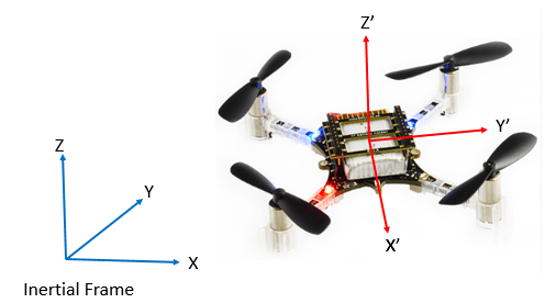
Refer to caption — Figure 2.1.1: Body-fixed frame and Inertial frame.

In the aeronautic systems, a popular axes convention is to define a positive altitude downwards, the Y axis pointing towards the east and the X axis pointing towards the true north. These types of frames are called NED frames (North, East, Down). It was decided to follow the convention used in the Crazyflie 2.0 firmware, meaning a positive altitude upwards, which defines an ENU frame (East, North, Up). Another remark is that the origin of the body-fixed frame matches with the center of gravity of the quadcopter.

Another important remark is knowing the flight configuration of the quadcopter as there are two of them: configuration “+” or configuration “X”. The difference between them is the orientation of the X-Y frame in terms of the arms of the quadcopter, as shown in Figure 2.1.2 taken from the manufacturer’s website [32] and modified accordingly.

In the modern conceptions of quadcopters the “X” configuration is prefered over the “+” configuration, mainly because in “X” it is easier to add a camera functionality as the quadcopter’s arms will not be interfering with the images captured. By default the Crazyflie 2.0 is in X mode, so for the rest of this project and during the mathematical modeling it will be considered that the quadcopter is in this configuration.

2.2 Dynamic Equations

The dynamic equations of the quadcopter proposed here take into account certain physical properties that are not necessarily perfectly valid in the real platform that is being used in this work, but they are good approximations that simplify greatly the study and comprehension of this type of vehicles. Here are the hypothesis:

1.

The quadcopter is a rigid body that cannot be deformed, thus it is possible to use the well-known dynamic equations of a rigid body.
2.

The quadcopter is symmetrical in its geometry, mass and propulsion system.
3.

The mass is constant (i.e its derivative is 0).

The mechanical classic laws of motion are valid in inertial systems, so to be able to translate these equations into the body frame it is necessary to define a rigid transformation matrix from the inertial frame to the body-fixed frame, in which only the rotational part is meaningful to the discussion and is given by three successive rotations: first a rotation of an angle $\psi$ around the $z$ axis, then a rotation of an angle $\theta$ around the intermediate $y$ axis and finally a rotation of an angle $\phi$ around the intermediate $x$ axis. Once these three rotations are calculated, the resulting transformation matrix is defined as:

$\bm{R}_{i}^{b}=\left[\begin{array}[]{ccc}\cos\theta\cos\psi&\cos\theta\sin\psi&-\sin\theta\\ \sin\phi\sin\theta\cos\psi-\cos\phi\sin\psi&\sin\phi\sin\theta\sin\psi+\cos\phi\cos\psi&\sin\phi\cos\theta\\ \cos\phi\sin\theta\cos\psi+\sin\phi\sin\psi&\cos\phi\sin\theta\sin\psi-\sin\phi\cos\psi&\cos\phi\cos\theta\end{array}\right]$

(2.2.1)

where $\phi$ , $\theta$ and $\psi$ represent the roll, pitch and yaw angles of the quadcopter’s body. Figure 2.2.1 shows the direction of said angles in the Crazyflie 2.0 body-fixed frame defined previously.

The notation convention used during the mathematical analysis of the quadcopter’s dynamics is exhibited in Table 2.2.1, where the state variables are defined.

Vector	State	Description
	$x$	X position of CoG in the inertial frame
$\bm{p}_{CG/o}$	$y$	Y position of CoG in the inertial frame
	$z$	Z position of CoG in the inertial frame
	$\phi$	Roll angle
$\bm{\Phi}$	$\theta$	Pitch angle
	$\psi$	Yaw angle
	$u$	X linear velocity of CoG in the body-fixed frame w.r to the inertial frame
$\bm{V}_{CG/o}$	$v$	Y linear velocity of CoG in the body-fixed frame w.r to the inertial frame
	$w$	Z linear velocity of CoG in the body-fixed frame w.r to the inertial frame
	$p$	Roll angular velocity in the body-fixed frame w.r to the inertial frame
$\bm{\omega}_{b/o}$	$q$	Pitch angular velocity in the body-fixed frame w.r to the inertial frame
	$r$	Yaw angular velocity in the body-fixed frame w.r to the inertial frame

w.r = with respect.

Table 2.2.1: Notation for vectors and states.

Furthermore, a left superindex such as $\vphantom{\dot{\bm{V}}_{CG/o}}{}^{o}\dot{\bm{V}}_{CG/o}$ will indicate in what frame a derivative is taken, while a right superindex indicate a vector coordinates into the specified frame. If a right superindex is not specified as in the example, then the vector does not experience any rotations after the derivative is taken.

2.2.1 Force Equations

According to Newton’s Second Law, the expression for the sum of forces is:

\sum\bm{F}=m\vphantom{\dot{\bm{V}}_{CG/o}}^{o}\dot{\bm{V}}_{CG/o}

(2.2.2)

The expression of this derivative of velocity can be determined using the Coriolis equation, which gives the following dynamic expression in the body-fixed frame:

\sum\bm{F}=m^{o}\dot{\bm{V}}_{CG/o}=m\left({}^{b}\dot{\bm{V}}_{CG/o}+\bm{\omega}_{b/o}\times\bm{V}_{CG/o}\right)

(2.2.3)

Each propeller of the quadcopter creates an aerodynamical force as shown in Figure 2.2.2 that acts upwards in the body-fixed frame.

In a situation where the quadcopter is parallel to the ground, meaning its roll and pitch angles are zero, the aerodynamic forces created by the propellers will search to counteract the effect of the weight and then make the quadcopter move upwards, downwards or stay in a hover position. In Figure 2.2.2 the vector “mg” actually represents the projection of the weight vector from the inertial frame to the body-fixed frame. That being said, this qualitative analysis of how the forces work in the quadcopter’s body can be translated into (2.2.3) as:

\left[\begin{array}[]{c}0\\ 0\\ F_{z}\end{array}\right]-\bm{R}_{o}^{b}\left[\begin{array}[]{c}0\\ 0\\ mg\end{array}\right]=m\left({\left[\begin{array}[]{c}\dot{u}\\ \dot{v}\\ \dot{w}\end{array}\right]}+\left[\begin{array}[]{c}p\\ q\\ r\end{array}\right]\times\left[\begin{array}[]{c}u\\ v\\ w\end{array}\right]\right)

(2.2.4)

From (2.2.4) it is possible to isolate the vector $\vphantom{\dot{\bm{V}}_{CG/o}}{}^{b}\dot{\bm{V}}_{CG/o}$ :

{\left[\begin{array}[]{c}\dot{u}\\ \dot{v}\\ \dot{w}\end{array}\right]}=\left[\begin{array}[]{c}0\\ 0\\ F_{z}/m\end{array}\right]-\bm{R}_{o}^{b}\left[\begin{array}[]{c}0\\ 0\\ g\end{array}\right]-\left[\begin{array}[]{c}p\\ q\\ r\end{array}\right]\times\left[\begin{array}[]{c}u\\ v\\ w\end{array}\right]

(2.2.5)

This equation dictates how the velocity of the center of gravity of the quadcopter evolves in its body-fixed frame. To determine another set of state space variables it is necessary to project this vector in the inertial frame to calculate the velocity in this coordinate system. Note: the matrix $\bm{R}_{o}^{b}$ is a rotation matrix, so it has the following property: $\left(\bm{R}_{o}^{b}\right)^{-1}=\left(\bm{R}_{o}^{b}\right){}^{T}=\bm{R}_{b}^{o}$ . Applying it, the projection is calculated:

\vphantom{\dot{\bm{p}}_{CG/o}^{b}}{}^{o}\dot{\bm{p}}_{CG/o}^{b}=\left(\bm{R}_{o}^{b}\right)\vphantom{\dot{\bm{p}}_{CG/o}}^{o}\dot{\bm{p}}_{CG/o}\Longleftrightarrow\vphantom{\dot{\bm{p}}_{CG/o}}^{o}\dot{\bm{p}}_{CG/o}=\bm{R}_{b}^{o}\bm{V}_{CG/o}^{b}\Longleftrightarrow{\left[\begin{array}[]{c}\dot{x}\\ \dot{y}\\ \dot{z}\end{array}\right]}=\bm{R}^{o}_{b}\left[\begin{array}[]{c}u\\ v\\ w\end{array}\right]

(2.2.6)

By integrating (2.2.6) it is possible to know the position of the quadcopter in the inertial frame.

Concerning the equations of forces and their state variables, it is necessary to specify the form of the aerodynamical force generated by the propellers. Following the diagram in Figure 2.2.2, the force generated by each propeller has the form:

\bm{F}_{i}^{b}=\left[\begin{array}[]{c}0\\ 0\\ T_{i}\end{array}\right]

(2.2.7)

where $T_{i}$ represents the upward thrust force in Newtons generated by each propeller. It is widely known that the thrust generated by a propeller is a function of the square of its angular speed:

T_{i}=C_{T}\omega_{i}^{2}

(2.2.8)

$C_{T}$ is a thrust coefficient that will be specified in Section 2.3 and $\omega_{i}$ is the rotation speed of the i-th motor, in revolutions per minute. As Figure 2.2.2 suggests, each propeller generates a thrust force following (2.2.8) and all in the same direction, which leads to a sum of all thrust forces:

\sum\bm{F}_{i}^{b}=\left[\begin{array}[]{c}0\\ 0\\ C_{T}\left(\omega_{1}^{2}+\omega_{2}^{2}+\omega_{3}^{2}+\omega_{4}^{2}\right)\end{array}\right]

(2.2.9)

2.2.2 Momentum Equations

These equations dictate the rotational dynamics of the quadcopter. Following the theorem of angular momentum:

\sum\bm{M}^{o}=\vphantom{\dot{\bm{h}}}^{o}\dot{\bm{h}}

(2.2.10)

where $\bm{h}$ denotes the angular momentum around the center of gravity. Using Coriolis equation:

\sum\bm{M}^{o}=\vphantom{\dot{\bm{h}}}^{o}\dot{\bm{h}}=\vphantom{\dot{\bm{h}}}^{b}\dot{\bm{h}}+\bm{\omega}_{b/o}\times\bm{h}

(2.2.11)

It is desirable to express (2.2.11) in the body-fixed frame as the momentum equations are more easily calculated, as explained in [31]:

\sum\bm{M}^{b}=\bm{J}\vphantom{\dot{\bm{\omega}}_{b/o}}^{b}\dot{\bm{\omega}}_{b/o}+\bm{\omega}_{b/o}\times\bm{J}\bm{\omega}_{b/o}

(2.2.12)

here $\bm{J}$ denotes the inertia matrix of the quadcopter, which in general can be expressed as:

\bm{J}=\left[\begin{array}[]{ccc}I_{xx}&-I_{xy}&-I_{xz}\\ -I_{xy}&I_{yy}&-I_{yz}\\ -I_{xz}&-I_{yz}&I_{zz}\end{array}\right]

(2.2.13)

but from the hypothesis that the body of the quadcopter is symmetrical around all its axes, the inertia matrix has all crossed terms equal to zero, i.e.,

\bm{J}=\left[\begin{array}[]{ccc}I_{xx}&0&0\\ 0&I_{yy}&0\\ 0&0&I_{zz}\end{array}\right]

(2.2.14)

From equation (2.2.12) it is possible to isolate the vector $\vphantom{\dot{\bm{\omega}}_{b/o}}{}^{b}\dot{\bm{\omega}}_{b/o}$ :

{\left[\begin{array}[]{c}\dot{p}\\ \dot{q}\\ \dot{r}\end{array}\right]}=\left(\bm{J}\right)^{-1}\left(\left[\begin{array}[]{c}M_{x}\\ M_{y}\\ M_{z}\end{array}\right]-\left[\begin{array}[]{c}p\\ q\\ r\end{array}\right]\times\bm{J}\left[\begin{array}[]{c}p\\ q\\ r\end{array}\right]\right)

(2.2.15)

The last state equations come from the relation between $\bm{\omega}_{b/o}$ and the Euler angles derivative $\dot{\bm{\Phi}}$

\left[\begin{array}[]{c}p\\ q\\ r\end{array}\right]=\left[\begin{array}[]{ccc}1&0&-\sin\theta\\ 0&\cos\phi&\sin\phi\cos\theta\\ 0&-\sin\phi&\cos\phi\cos\theta\end{array}\right]\left[\begin{array}[]{c}\dot{\phi}\\ \dot{\theta}\\ \dot{\psi}\end{array}\right]

(2.2.16)

with the inverse relation the state vector $\dot{\bm{\Phi}}$ is isolated:

\hskip 62.59596pt\left[\begin{array}[]{c}\dot{\phi}\\ \dot{\theta}\\ \dot{\psi}\end{array}\right]=\left[\begin{array}[]{ccc}1&\sin\phi\tan\theta&\cos\phi\tan\theta\\ 0&\cos\phi&-\sin\phi\\ 0&\sin\phi/\cos\theta&\cos\phi/\cos\theta\end{array}\right]\left[\begin{array}[]{c}p\\ q\\ r\end{array}\right]\,\textrm{for}\,\theta\neq\frac{\pi}{2}

(2.2.17)

To calculare the total momentum generated in the quadcopter system, it is imperative to know the rotation direction of each motor. As seen in Figure 2.2.3, the manufacturer of the Crazyflie 2.0 provides this information [32].

The expression for the momentum is given as:

\bm{M}=\sum_{i=1}^{4}\bm{P}_{i}\times\bm{F}_{i}+\sum_{i=1}^{4}\bm{\tau}_{i}

(2.2.18)

where $\bm{P}_{i}$ represents the position of each motor in the body-fixed frame and $\bm{\tau}_{i}$ represents the induced momentum in the quadcopter’s body generated by the i-th motor. When a rotor turns in a given direction, conservation of angular momentum dictates that the quadcopter’s body will have a tendency to counteract the generated angular momentum, being consistent with Newton’s third law of action and reaction. This reaction momentum due to the spin of a rotor is the induced moment $\bm{\tau}_{i}$ .

If $d$ denotes the distance from the center of gravity to the center of each motor, the position of each motor is:

$\bm{P}_{1}=\left[\begin{array}[]{c}d/\sqrt{2}\\ -d/\sqrt{2}\\ 0\end{array}\right]\text{ },\text{ }\bm{P}_{2}=\left[\begin{array}[]{c}-d/\sqrt{2}\\ -d/\sqrt{2}\\ 0\end{array}\right]\text{ },\text{ }\bm{P}_{3}=\left[\begin{array}[]{c}-d/\sqrt{2}\\ d/\sqrt{2}\\ 0\end{array}\right]\text{ },\text{ }\bm{P}_{4}=\left[\begin{array}[]{c}d/\sqrt{2}\\ d/\sqrt{2}\\ 0\end{array}\right]$

(2.2.19)

Then the mometum generated by the thrust force of each motor can be calculated:

$\bm{P}_{1}^{b}\times\bm{F}_{1}^{b}=\left[\begin{array}[]{c}\left(-C_{T}\omega_{1}^{2}\right)d/\sqrt{2}\\ \left(-C_{T}\omega_{1}^{2}\right)d/\sqrt{2}\\ 0\end{array}\right]$ $\bm{P}_{2}^{b}\times\bm{F}_{2}^{b}=\left[\begin{array}[]{c}\left(-C_{T}\omega_{2}^{2}\right)d/\sqrt{2}\\ \left(C_{T}\omega_{2}^{2}\right)d/\sqrt{2}\\ 0\end{array}\right]$

$\bm{P}_{3}^{b}\times\bm{F}_{3}^{b}=\left[\begin{array}[]{c}\left(C_{T}\omega_{3}^{2}\right)d/\sqrt{2}\\ \left(C_{T}\omega_{3}^{2}\right)d/\sqrt{2}\\ 0\end{array}\right]$ $\bm{P}_{4}^{b}\times\bm{F}_{4}^{b}=\left[\begin{array}[]{c}\left(C_{T}\omega_{4}^{2}\right)d/\sqrt{2}\\ \left(-C_{T}\omega_{4}^{2}\right)d/\sqrt{2}\\ 0\end{array}\right]$

The induced moments $\bm{\tau}_{i}$ act only in the Z axis and have an opposite magnitude from the moment generated by each propeller, due to the conservation of angular momentum. In this particular case, given the axis convention that is being used (z axis pointing upwards), applying the right-hand rule indicate that a clockwise spinning rotor yields a negative momentum (one thumb points downward, in the opposite direction of the z axis), thus the induced momentum will be positive. Then, the sum of induced moments in the quadcopter’s body is calculated:

\sum_{i=1}^{4}\bm{\tau}_{i}^{b}=\left[\begin{array}[]{c}0\\ 0\\ C_{D}\left(-\omega_{1}^{2}+\omega_{2}^{2}-\omega_{3}^{2}+\omega_{4}^{2}\right)\end{array}\right]

(2.2.20)

where $C_{D}$ denotes the aerodynamic drag coefficient that will be specified in Section 2.3. Finally, the total moment has the following form:

\bm{M}^{b}=\left[\begin{array}[]{c}M_{x}\\ M_{y}\\ M_{z}\end{array}\right]=\left[\begin{array}[]{c}dC_{T}/\sqrt{2}\left(-\omega_{1}^{2}-\omega_{2}^{2}+\omega_{3}^{2}+\omega_{4}^{2}\right)\\ dC_{T}/\sqrt{2}\left(-\omega_{1}^{2}+\omega_{2}^{2}+\omega_{3}^{2}-\omega_{4}^{2}\right)\\ C_{D}\left(-\omega_{1}^{2}+\omega_{2}^{2}-\omega_{3}^{2}+\omega_{4}^{2}\right)\end{array}\right]

(2.2.21)

In the total momentum equation there are certain terms that include angular accelerations that have been neglected as they tend to be small compared to the other terms of the equation. Gyroscopic moments have also been neglected using the argument that the inertia moment of each motor tends to be small thus their contribution in the total momentum is also small [21, 30].

2.3 Physical Parameters

The precise measurement of certain physical parameters is the key to create a simulation environment that correctly describes the behavior of the quadcopter. In [1] a study of said physical parameters was undertaken for the Crazyflie 2.0. The aerodynamical coefficients were studied in [2] for the Crazyflie 1.0, but they are the same or at least close to those of the Crazyflie 2.0 given the fact that these coefficients only depend on the geometry of the propellers [3], which remained unchanged between the two models. Results of both works are summarized in Table 2.3.1.

Parameter	Description	Value
$m_{quad}$	Mass of the quadcopter alone	$0.27\,[\textrm{Kg}]$
$m_{uwb}$	Mass of the UWB module	$0.04\,[\textrm{Kg}]$
$m_{vicon}$	Mass of one VICON marker	$0.02\,[\textrm{Kg}]$
$m$	Total mass	$0.33\,[\textrm{Kg}]$
$d$	Arm length	$39.73\times 10^{-3}\,[\textrm{m}]$
$r$	Rotor radius	$23.1348\times 10^{-3}\,[\textrm{m}]$
$I_{xx}$	Principal Moment of Inertia around x axis	$1.395\times 10^{-5}\,[\textrm{Kg}\times\textrm{m}^{2}]$
$I_{yy}$	Principal Moment of Inertia around y axis	$1.436\times 10^{-5}\,[\textrm{Kg}\times\textrm{m}^{2}]$
$I_{zz}$	Principal Moment of Inertia around z axis	$2.173\times 10^{-5}\,[\textrm{Kg}\times\textrm{m}^{2}]$
$k_{T}$	Non-dimensional thrust coefficient	$0.2025$
$k_{D}$	Non-dimensional torque coefficient	$0.11$

Table 2.3.1: Physical parameters for the Crazyflie 2.0.

In addition, as explained in [3], the thrust generated by the propeller is often expressed as:

T=k_{T}\rho n^{2}D^{4}

(2.3.1)

where $k_{T}$ is the non-dimensional thrust coefficient, $\rho$ is the density of air, $n$ is the propeller speed in revolutions per second and $D$ is the diameter of the rotor. As it will be evident later, it is convenient to express the propeller speed in RPM’s. Knowing that 1 revolution per second is the same as 60 revolutions per minute, (2.3.1) becomes:

T=k_{T}\mbox{$\rho$}\left(\omega/60\right)^{2}D^{4}

(2.3.2)

where $\omega$ is the angular speed of the propeller in RPM. Comparing the above with (2.2.8), it is possible to determine the thrust coefficient $C_{T}$ as:

C_{T}=k_{T}\rho\left(2r\right)^{4}/3600

(2.3.3)

taking the value of air density constant $\rho=1.225\,[\textrm{Kg/m}^{3}]$ and all the other constants defined previously, finally this coefficient is:

\boxed{C_{T}=3.1582\times 10^{-10}\,[\textrm{N/rpm}^{2}]}

(2.3.4)

Now for the torque coefficient, as specified in [3], the torque created by the propellers is described by this equation:

Q=k_{D}\rho n^{2}D^{5}

(2.3.5)

Operating the same variable change as in (2.3.3), then:

C_{D}=k_{D}\rho\left(2r\right)^{5}/3600

(2.3.6)

\boxed{C_{D}=7.9379\times 10^{-12}\,[\textrm{Nm/rpm}^{2}]}

(2.3.7)

With the parameters specified in Table 2.3.1 and the constants calculated in (2.3.4) and (2.3.7), all the basic physical parameters were determined. Here we use the word “basic” as these parameters are the minimum necessary to be able to simulate the behavior of a quadcopter and because in most applications, this one included, are a good approximation of the real physical system.

2.4 Linearization and State Space Representation

The state space representation of a system gives an idea of how the system evolves in time by the following equations:

\begin{cases}\dot{\bm{x}}\left(t\right)=\bm{A}\left(t\right)\bm{x}\left(t\right)+\bm{B}\left(t\right)\bm{u}\left(t\right)\\ \bm{y}\left(t\right)=\bm{C}\left(t\right)\bm{x}\left(t\right)+\bm{D}\left(t\right)\bm{u}\left(t\right)\end{cases}

(2.4.1)

In general, this equation describes the evolution of a linear time-varying system, where $\bm{x}\left(t\right)$ is the vector of states, $\bm{y}\left(t\right)$ is the output vector and $\bm{u}\left(t\right)$ is the input vector. For the state space representation of a quadcopter it is conventional to consider the following linear time-invariant realisation of the system, meaning that matrices A, B, C and D are static and don’t change over time:

\begin{cases}\Delta\dot{\bm{x}}=\bm{A}\Delta\bm{x}+\bm{B}\Delta\bm{u}\\ \Delta\bm{y}=\bm{C}\Delta\bm{x}+\bm{D}\Delta\bm{u}\end{cases}

(2.4.2)

where the prefix $\Delta$ means that the vector is the result of a linearisation process.

When linearizing a system the important question becomes at around which so-called "trim" trajectory we desire to linearize, or better yet, what is the trim trajectory most well-suited given the needs of the system. This trim trajectory has to be associated with an equilibrium point in which the states of the system do not change over time, meaning $\dot{\bm{x}}_{e}=0$ . In the case of the quadcopter, the common trim trajectory is the hover, in which the drone stays stationary at a certain altitude. This fact can be translated as an equilibrium state:

\bm{x}_{e}=\left[\begin{array}[]{cccccccccccc}x_{e}&y_{e}&z_{e}&\psi_{e}&\theta_{e}&\phi_{e}&u_{e}&v_{e}&w_{e}&r_{e}&q_{e}&p_{e}\end{array}\right]^{T}

(2.4.3)

At the equilibrium point, the quadcopter’s linear position and yaw angle are indifferent in terms of the linearization calculus, so they can be considered arbitrary constants. For the roll and pitch angles, they need to be zero in order for the quadcopter to keep the stationary position, and so does any linear or angular velocity. Finally the equilibrium vector is as simple as:

\bm{x}_{e}=\left[\begin{array}[]{cccccccccccc}x_{e}&y_{e}&z_{e}&\psi_{e}&0&0&0&0&0&0&0&0\end{array}\right]^{T}

(2.4.4)

In order to keep the quadcopter flying in hover mode, knowing that the body is levelled with the floor and there are no gravity components other that in the z axis, the force generated by the propellers need to compensate exactly for the weight of the quadcopter to stay stationary in the air, this means:

C_{T}\left(\omega_{e1}^{2}+\omega_{e2}^{2}+\omega_{e3}^{2}+\omega_{e4}^{2}\right)=mg

(2.4.5)

From the hypothesis that the quadcopter’s body is perfectly symmetrical, a quick deduction is that all motors need to rotate with the same speed in order to maintain the body levelled and don’t create any angular momentum, this means that in equilibrium:

\omega_{e1}=\omega_{e2}=\omega_{e3}=\omega_{e4}=\omega_{e}

(2.4.6)

Combining (2.4.5) and eqrefeq:32 gives as result:

\boxed{\omega_{e}=\sqrt{\frac{mg}{4C_{T}}}=16073\,\textrm{[rpm]}}

(2.4.7)

This constant specifies the required speed of each rotor in order to maintain the hover position and so the input vector in equilibrium is:

u_{e}=\left[\begin{array}[]{cccc}\omega_{e}&\omega_{e}&\omega_{e}&\omega_{e}\end{array}\right]^{T}

(2.4.8)

After applying a Taylor’s first order expansion, and taking into account the equilibrium state vector specified in (2.4.4), the linearized equations are:

\begin{cases}\Delta F_{x}=m\Delta\dot{u}-mg\Delta\theta\\ \Delta F_{y}=m\Delta\dot{v}+mg\Delta\phi\\ \Delta F_{z}=m\Delta\dot{w}\\ \Delta M_{x}=I_{xx}\Delta\dot{p}\\ \Delta M_{y}=I_{yy}\Delta\dot{q}\\ \Delta M_{z}=I_{zz}\Delta\dot{r}\end{cases}

(2.4.9)

The linearized forces and moments are:

\bm{\Delta F}^{b}=\left[\begin{array}[]{c}\Delta F_{x}\\ \Delta F_{y}\\ \Delta F_{z}\end{array}\right]=\left[\begin{array}[]{c}0\\ 0\\ 2C_{T}\omega_{e}\left(\Delta\omega_{1}+\Delta\omega_{2}+\Delta\omega_{3}+\Delta\omega_{4}\right)\end{array}\right]

(2.4.10)

\bm{\Delta M}^{b}=\left[\begin{array}[]{c}\Delta M_{x}\\ \Delta M_{y}\\ \Delta M_{z}\end{array}\right]=\left[\begin{array}[]{c}\sqrt{2}dC_{T}\omega_{e}\left(-\Delta\omega_{1}-\Delta\omega_{2}+\Delta\omega_{3}+\Delta\omega_{4}\right)\\ \sqrt{2}dC_{T}\omega_{e}\left(-\Delta\omega_{1}+\Delta\omega_{2}+\Delta\omega_{3}-\Delta\omega_{4}\right)\\ 2C_{D}\omega_{e}\left(-\Delta\omega_{1}+\Delta\omega_{2}-\Delta\omega_{3}+\Delta\omega_{4}\right)\end{array}\right]

(2.4.11)

In hover position the body-fixed frame coincides with the inertial frame, meaning:

\begin{cases}\Delta\dot{x}=\Delta u\\ \Delta\dot{y}=\Delta v\\ \Delta\dot{z}=\Delta w\end{cases}\,\,\,\,\,\,\,\,\,\,\,\,\,\,\,\,\,\begin{cases}\Delta\dot{\phi}=\Delta p\\ \Delta\dot{\theta}=\Delta q\\ \Delta\dot{\psi}=\Delta r\end{cases}

(2.4.12)

Merging (2.4.9) to (2.4.12) allows to write the state space representation of the linearized quadcopter:

$\left[\begin{array}[]{c}\Delta\dot{x}\\ \Delta\dot{y}\\ \Delta\dot{z}\\ \Delta\dot{\psi}\\ \Delta\dot{\theta}\\ \Delta\dot{\phi}\\ \Delta\dot{u}\\ \Delta\dot{v}\\ \Delta\dot{w}\\ \Delta\dot{r}\\ \Delta\dot{q}\\ \Delta\dot{p}\end{array}\right]=\left[\begin{array}[]{cccccccccccc}0&0&0&0&0&0&1&0&0&0&0&0\\ 0&0&0&0&0&0&0&1&0&0&0&0\\ 0&0&0&0&0&0&0&0&1&0&0&0\\ 0&0&0&0&0&0&0&0&0&1&0&0\\ 0&0&0&0&0&0&0&0&0&0&1&0\\ 0&0&0&0&0&0&0&0&0&0&0&1\\ 0&0&0&0&g&0&0&0&0&0&0&0\\ 0&0&0&0&0&-g&0&0&0&0&0&0\\ 0&0&0&0&0&0&0&0&0&0&0&0\\ 0&0&0&0&0&0&0&0&0&0&0&0\\ 0&0&0&0&0&0&0&0&0&0&0&0\\ 0&0&0&0&0&0&0&0&0&0&0&0\end{array}\right]\left[\begin{array}[]{c}\Delta x\\ \Delta y\\ \Delta z\\ \Delta\psi\\ \Delta\theta\\ \Delta\phi\\ \Delta u\\ \Delta v\\ \Delta w\\ \Delta r\\ \Delta q\\ \Delta p\end{array}\right]+\omega_{e}\left[\begin{array}[]{cccc}0&0&0&0\\ 0&0&0&0\\ 0&0&0&0\\ 0&0&0&0\\ 0&0&0&0\\ 0&0&0&0\\ 0&0&0&0\\ 0&0&0&0\\ 2C_{T}/m&2C_{T}/m&2C_{T}/m&2C_{T}/m\\ -2C_{D}/I_{zz}&2C_{D}/I_{zz}&-2C_{D}/I_{zz}&2C_{D}/I_{zz}\\ -\sqrt{2}dC_{T}/I_{yy}&\sqrt{2}dC_{T}/I_{yy}&\sqrt{2}dC_{T}/I_{yy}&-\sqrt{2}dC_{T}/I_{yy}\\ -\sqrt{2}dC_{T}/I_{xx}&-\sqrt{2}dC_{T}/I_{xx}&\sqrt{2}dC_{T}/I_{xx}&\sqrt{2}dC_{T}/I_{xx}\end{array}\right]$ $\left[\begin{array}[]{c}\Delta\omega_{1}\\ \Delta\omega_{2}\\ \Delta\omega_{3}\\ \Delta\omega_{4}\end{array}\right]$

2.5 Movement Decoupling

In the state space realization of the quadcopter’s linear model, the four inputs of the system act directly in just four states of the system. Rewriting together (2.4.10) and (2.4.11) show how each input of the system contributes to each force and momentum.

\left[\begin{array}[]{c}F_{z}\\ M_{x}\\ M_{y}\\ M_{z}\end{array}\right]=2\omega_{e}\left[\begin{array}[]{cccc}C_{T}&C_{T}&C_{T}&C_{T}\\ -dC_{T}/\sqrt{2}&-dC_{T}/\sqrt{2}&dC_{T}/\sqrt{2}&dC_{T}/\sqrt{2}\\ -dC_{T}/\sqrt{2}&dC_{T}/\sqrt{2}&dC_{T}/\sqrt{2}&-dC_{T}/\sqrt{2}\\ -C_{D}&C_{D}&-C_{D}&C_{D}\end{array}\right]\left[\begin{array}[]{c}\Delta\omega_{1}\\ \Delta\omega_{2}\\ \Delta\omega_{3}\\ \Delta\omega_{4}\end{array}\right]

(2.5.1)

From (2.5.1) a transformation matrix can be defined between the forces acting on the quadcopter’s body and the angular speed from the motors:

\bm{\Gamma}=2\omega_{e}\left[\begin{array}[]{cccc}C_{T}&C_{T}&C_{T}&C_{T}\\ -dC_{T}/\sqrt{2}&-dC_{T}/\sqrt{2}&dC_{T}/\sqrt{2}&dC_{T}/\sqrt{2}\\ -dC_{T}/\sqrt{2}&dC_{T}/\sqrt{2}&dC_{T}/\sqrt{2}&-dC_{T}/\sqrt{2}\\ -C_{D}&C_{D}&-C_{D}&C_{D}\end{array}\right]

(2.5.2)

If matrix $\bm{\Gamma}$ is invertible (i.e: $\bm{\Gamma}^{-1}$ exists) that means that all four lines are independent and thus the vertical and angular forces of the quadcopter act independently from each other. Inverting the matrix:

\bm{\Gamma}^{-1}=\frac{1}{2\omega_{e}}\left[\begin{array}[]{cccc}1/\left(4C_{T}\right)&-\sqrt{2}/\left(4dC_{T}\right)&-\sqrt{2}/\left(4dC_{T}\right)&-1/\left(4C_{D}\right)\\ 1/\left(4C_{T}\right)&-\sqrt{2}/\left(4dC_{T}\right)&\sqrt{2}/\left(4dC_{T}\right)&1/\left(4C_{D}\right)\\ 1/\left(4C_{T}\right)&\sqrt{2}/\left(4dC_{T}\right)&\sqrt{2}/\left(4dC_{T}\right)&-1/\left(4C_{D}\right)\\ 1/\left(4C_{T}\right)&\sqrt{2}/\left(4dC_{T}\right)&-\sqrt{2}/\left(4dC_{T}\right)&1/\left(4C_{D}\right)\end{array}\right]

(2.5.3)

Now taking the result in (2.5.3), it is possible to find the inverse relation of (2.5.1):

$\left[\begin{array}[]{c}\Delta\omega_{1}\\ \Delta\omega_{2}\\ \Delta\omega_{3}\\ \Delta\omega_{4}\end{array}\right]=\frac{1}{2\omega_{e}}\left[\begin{array}[]{cccc}1/\left(4C_{T}\right)&-\sqrt{2}/\left(4dC_{T}\right)&-\sqrt{2}/\left(4dC_{T}\right)&-1/\left(4C_{D}\right)\\ 1/\left(4C_{T}\right)&-\sqrt{2}/\left(4dC_{T}\right)&\sqrt{2}/\left(4dC_{T}\right)&1/\left(4C_{D}\right)\\ 1/\left(4C_{T}\right)&\sqrt{2}/\left(4dC_{T}\right)&\sqrt{2}/\left(4dC_{T}\right)&-1/\left(4C_{D}\right)\\ 1/\left(4C_{T}\right)&\sqrt{2}/\left(4dC_{T}\right)&-\sqrt{2}/\left(4dC_{T}\right)&1/\left(4C_{D}\right)\end{array}\right]\left[\begin{array}[]{c}F_{z}\\ M_{x}\\ M_{y}\\ M_{z}\end{array}\right]$

(2.5.4)

Equation (2.5.4) dictates how each motor contributes to each of the forces acting on the quadcopter’s body. This study confirms that the vertical, lateral, longitudinal and directional (yaw) forces act independently from each other in the mathematical model and thus the quadcopter’s dynamics are decoupled and can be studied as sub-systems.

•

Vertical Subsystem

This subsystem describes the dynamics of the upward movements of the quadcopter, following this state space equation:

\left[\begin{array}[]{c}\Delta\dot{w}\\ \Delta\dot{z}\end{array}\right]=\left[\begin{array}[]{cc}0&0\\ 1&0\end{array}\right]\left[\begin{array}[]{c}\Delta w\\ \Delta z\end{array}\right]+\left[\begin{array}[]{c}1/m\\ 0\end{array}\right]\Delta F_{z}

(2.5.5)

•

Directional Subsystem

The yaw angle and its velocity dictate the dynamics of the quadcopter direction in the XY plane, as suggests this following state space equation:

\left[\begin{array}[]{c}\Delta\dot{r}\\ \Delta\dot{\psi}\end{array}\right]=\left[\begin{array}[]{cc}0&0\\ 1&0\end{array}\right]\left[\begin{array}[]{c}\Delta r\\ \Delta\psi\end{array}\right]+\left[\begin{array}[]{c}1/I_{zz}\\ 0\end{array}\right]\Delta M_{z}

(2.5.6)

•

Lateral Subsystem

The lateral dynamic governs the pitch movement of the quadcopter, as well as its Y position in the inertial frame:

\left[\begin{array}[]{c}\Delta\dot{p}\\ \Delta\dot{\phi}\\ \Delta\dot{v}\\ \Delta\dot{y}\end{array}\right]=\left[\begin{array}[]{cccc}0&0&0&0\\ 1&0&0&0\\ 0&-g&0&0\\ 0&0&1&0\end{array}\right]\left[\begin{array}[]{c}\Delta p\\ \Delta\phi\\ \Delta v\\ \Delta y\end{array}\right]+\left[\begin{array}[]{c}1/I_{xx}\\ 0\\ 0\\ 0\end{array}\right]\Delta M_{x}

(2.5.7)

•

Longitudinal Subsystem

Similar to the lateral subsystem, it rules the movement around the X axis of the body-fixed frame of the quadcopter, and its X position and velocity in the inertial frame.

\left[\begin{array}[]{c}\Delta\dot{q}\\ \Delta\dot{\theta}\\ \Delta\dot{u}\\ \Delta\dot{x}\end{array}\right]=\left[\begin{array}[]{cccc}0&0&0&0\\ 1&0&0&0\\ 0&g&0&0\\ 0&0&1&0\end{array}\right]\left[\begin{array}[]{c}\Delta q\\ \Delta\theta\\ \Delta u\\ \Delta x\end{array}\right]+\left[\begin{array}[]{c}1/I_{yy}\\ 0\\ 0\\ 0\end{array}\right]\Delta M_{x}

(2.5.8)

2.6 Motor Characterization

The inputs of the above state space realization are the angular speed of each motor in RPM’s, but after exploring the Crazyflie’s 2.0 firmware it became evident that this is not the real input of the system. The voltage sent to each DC motor is controlled using a PWM signal specified as a 16 bit number, ranging from 0 to 65535, meaning that the actual input of the system can be considered directly as this PWM signal and not the actual voltage sent to the motors. In [2] experimental data was retrieved from the motors to identify the relationship between the PWM signal sent to the motors and the RPM’s generated. The experiments proved that the angular speed of the motors have a linear relationship with the PWM input of the system, following the equation:

RPM=0.2685\times PWM+4070.3

(2.6.1)

The characterization of a DC motor usually derives in a first order transfer function that specifies certain response time from the motors as they do not react immediately to the commands sent, but it is a good approximation to assume that this response time is fast enough and that it will not cause much delays in the system, thus (2.6.1) serves as a good approximation for the motor characterization.

Chapter 3 Simulation

In this section a simulation environment of the quadcopter’s dynamics is proposed with the intention of testing and designing control schemes. Two different controllers are proposed: in the first phase of the project a position PID tracker was considered and in a second phase a trajectory tracker known as the Linear-Quadratic Tracker (LQT) was studied.

3.1 Cascaded PID Position Tracker

Figure 3.1.1presents the simulation model created for this phase of the project.

Figure 3.1.1: Block Diagram of Simulation environment.

Now an explanation of each simulation block will be given:

1.

Trajectory: this block serves as the input of the overall system, specifying a trajectory in the x,y,z and yaw positions. As of now the commands sent by this block are mere constants or signal inputs such as sinusoids, random signals, ramps, etc. It serves as input commands to the controller.
2.

Controller: takes the desired trajectory and the quadcopter’s states as inputs and computes the necessary 16-bit PWM signal to send to the motors.
3.

Motors: implements the linear relation between the 16-bit PWM signal sent to the motors and the actual angular speed in revolutions per minutes generated by them, as specified in Section 2.6.
4.

Quadcopter’s dynamics: this block implements the dynamic equations of Section 2.2. The vectorial form of the equations, as they were developed, is the simplest, most common and elegant way of constructing this block. The non-linear model was linearized using MATLAB’s command “linmod” to verify it was consistent with the theoretical state space model found in the previous section.
5.

Sensor’s noise: allows to add additive white Gaussian noise to specific states of the quadcopters, to simulate the sensors that give the real states used by the control system. This block could be modified by the user to define more complex models, e.g., including sensor bias.

3.1.1 On-Board Control Architecture

The first steps to control the quadcopter was understanding the already implemented controllers that came with the stock firmware of the Crazyflie 2.0 (Firmware release 2016.02). As seen in Figure 3.1.2 the manufacturers specify the control architecture used:

A two cascaded PID control scheme was found in the Crazyflie’s firmware in order to control the pitch and roll angles. A cascaded control structure can be analysed by decomposing the architecture in an inner and outer control loops, in which the outer loop regulates the inner loop, which in turn regulates the plant of the system. As a common rule in cascaded structures, the inner loop needs to regulate at a faster rate than the outer loop. It is ideal for the inner loop output to reach an steady state value before the outer loop changes the setpoint sent to the inner loop. Synchronization problems will occur between the two controllers if the inner loop response is not as fast as it should, or if the outer loop is faster than it should. In implementation terms this is easily remediable by forcing the inner loop to be, as in this case, twice as fast as the outer loop (Attitude controller running at 250Hz and Rate controller running at 500Hz).

3.1.1.1 Inner Loop: Rate Controller

The inputs and outputs of this block are shown in Figure 3.1.3.

Figure 3.1.3: Rate Controller diagram.

The goal of this controller is to calculate the input variation from the equilibrium point of the motors in order to create the angular momentum required for the state variables $p$ , $q$ and $r$ to get the values $p_{c}$ , $q_{c}$ and $r_{c}$ respectively. For that, three independent controllers are used:

•

Roll Rate Proportional controller: calculates $\Delta_{\phi}$ following this equation, the desired value $p_{c}$ is calculated by the outer loop attitude controller:

$\Delta_{\phi}\left(t\right)=K_{P,p}\left(p_{c}\left(t\right)-p\left(t\right)\right)$ (3.1.1)
•

Pitch Rate Proportional controller: very similar to the roll rate controller, calculates $\Delta_{\theta}$ from the setpoint value $q_{c}$ :

$\Delta_{\theta}\left(t\right)=K_{P,q}\left(q_{c}\left(t\right)-q\left(t\right)\right)$ (3.1.2)

•

Yaw Rate Proportional-Integral controller: calculates the desired deviation from the base thrust, $\Delta_{\psi}$ , from an external setpoint $r_{c}$ that can be specified through a teleoperation system or as it is going to be specified later, by an off-board controller. The control law for this compensator is:

\Delta_{\theta}\left(t\right)=K_{P,r}\left(r_{c}\left(t\right)-r\left(t\right)\right)+K_{I,r}\int_{0}^{t}\left(r_{c}\left(\tau\right)-r\left(\tau\right)\right)d\tau

(3.1.3)

Table 3.1.1contains the gains for each of these controllers, taken directly from the Crazyflie’s firmware.

Controller	$K_{P}$	$K_{I}$
Roll Rate	$70$	-
Pitch Rate	$70$	-
Yaw Rate	$70$	$16.7$

Table 3.1.1: Rate Controller’s gains.

3.1.1.2 Outer Loop: Attitude Controller

The inputs and outputs of the attitude controller are as show in Figure 3.1.4.

Figure 3.1.4: Rate Controller diagram.

This controller act as a regulator of the rate controller, calculating the appropriate setpoints for the angular velocities around the X and Y axis, in order to stabilize the quadcopter at a certain desired angular position. The attitude controller uses the pitch and roll angles estimates from the sensor fusion algorithm, compares them to the external commands $\phi_{c}$ and $\theta_{c}$ (coming from teleoperation, off-board controller, etc) and feeds them to a controller that calculates the desired angular velocities $p_{c}$ and $q_{c}$ . These controllers are as follows:

•

Roll Attitude Proportional-Integral controller: computes the desired roll rate in the body frame, $p_{c}$ ,using the control law:

p_{c}\left(t\right)=K_{P,\phi}\left(\phi_{c}\left(t\right)-\phi\left(t\right)\right)+K_{I,\phi}\int_{0}^{t}\left(\phi_{c}\left(\tau\right)-\phi\left(\tau\right)\right)d\tau

(3.1.4)

•

Pitch Attitude Proportional-Integral controller: works in the same fashion as the roll controller, using the corresponding variables:

q_{c}\left(t\right)=K_{P,\theta}\left(\theta_{c}\left(t\right)-\theta\left(t\right)\right)+K_{I,\theta}\int_{0}^{t}\left(\theta_{c}\left(\tau\right)-\theta\left(\tau\right)\right)d\tau

(3.1.5)

Once again, the gains for these controllers were already specified in the Crazyflie’s firmware release 2016.02, as seen in Table 3.1.2. The same values were used during this project as they turned out to be well tuned according to the simulations and the tests made with the real platform.

Controller	$K_{P}$	$K_{I}$
Roll Attitude	$3.5$	$2$
Pitch Attitude	$3.5$	$2$

Table 3.1.2: Attitude Controller’s gains.

As it is evident from the gain values in Tables 3.1.1 and 3.1.2, the roll and pitch gains for both controllers are the same, which is consistent with the initial hypothesis that the quadcopter is a symmetrical body around all its axes.

3.1.1.3 Control Mixer

The output of the rate controller is the total input variation of the motors from the equilibrium state required to generate a torque in the desired direction of movement. Afterwards this input variation has to be distributed to the motors in the same fashion as in (2.4.11), for it to move and rotate appropriately using the PWM input it received. Given that the quadcopter is in X configuration, the motor effort has to be distributed halfway in each motor for a desired torque around the X or Y axis. All this analysis can be translated in the following equations that are implemented on board of the Crazyflie 2.0, thus specifying a “Control mixer” block in the simulation environment:

\begin{cases}PWM_{motor_{1}}=&\Omega-\Delta_{\phi}/2-\Delta_{\theta}/2-\Delta_{\psi}\\ PWM_{motor_{2}}=&\Omega+\Delta_{\phi}/2-\Delta_{\theta}/2+\Delta_{\psi}\\ PWM_{motor_{3}}=&\Omega+\Delta_{\phi}/2+\Delta_{\theta}/2-\Delta_{\psi}\\ PWM_{motor_{4}}=&\Omega-\Delta_{\phi}/2-\Delta_{\theta}/2+\Delta_{\psi}\end{cases}

(3.1.6)

where $\Omega$ is the PWM base signal for maintaining a certain altitude, a value that will be regulated from an altitude controller; $\Delta_{\phi}$ , $\Delta_{\theta}$ and $\Delta_{\psi}$ represent the outputs of the Rate Controller and at the same time give an idea of a deviation needed from the base thrust in order to obtain a certain torque in the X, Y or Z axis. From (3.1.6) it is more clearly how, for example, a command $\Delta_{\phi}>0$ will be distributed 50/50 as a reduction of the PWM input supplied to motors 1 and 4, and an increase of the power supplied to motors 2 and 3, thus creating the appropriate angular momentum to obtain certain angle in the pitch direction.

Figure 3.1.5 shows a complete diagram of the on-board control scheme.

Figure 3.1.5: Onboard control architecture with Control mixer.

The red inputs in this diagram represent the actual inputs that can be controlled from outside of the firmware, as it was suggested earlier, either by a teleoperation system or by an automated position controller. The other signals come from the sensor fusion algorithm or are intermediate variables in the control process.

3.1.2 Off-Board Position Controller

In hopes of controlling the quadcopter by sending waypoints or trajectories in a tridimensional space, it became necessary to add a position controller that in terms of the implementation will be running off-board unlike the controller of the previous section. The job of this controller can be divided into:

1.

An altitude controller whose output is the thrust $\Omega$ required to maintain a certain position in z.
2.

An X-Y position controller whose outputs are the required roll and pitch angles that will be regulated by the on-board controller.
3.

A yaw position controller that sends the required angular velocity to the on-board Yaw Rate Controller.

As seen in the dynamic analysis of the quadcopter, there exists a theoretical decoupling between the vertical, lateral, longitudinal and yaw movement, meaning that each one of these controllers can be tuned independently from each other, which simplifies the controller design task.

3.1.2.1 Altitude Controller

It is common practice to add a feedforward term as in [4] that compensates the weight of the quadcopter, in order to avoid the use of large controller gains that can lead to saturation problems. The structure in Figure 3.1.6 was the one used for this controller.

Figure 3.1.6: Altitude Controller.

The altitude controller is a simple PID compensator whose inputs are the desired altitude that comes from the trajectory block, and the altitude state that in terms of simulation comes from the quadcopter’s dynamics block. The equation that describes this PID controller is the following:

$\Delta\Omega\left(t\right)=K_{P,z}\left(z_{c}\left(t\right)-z\left(t\right)\right)+K_{I,z}\int_{0}^{t}\left(z_{c}\left(\tau\right)-z\left(\tau\right)\right)d\tau+K_{D,z}\frac{d}{dt}\left(z_{c}\left(t\right)-z\left(t\right)\right)$

(3.1.7)

The output of this PID controller is the 16-bit thrust deviation from the equilibrium point set at the hover state. That means that the feedforward term $\Omega_{e}$ in Figure 3.1.6 is the necessary PWM 16-bit signal needed for the quad to maintain its altitude. Using the calculations at the equilibrium, as seen in (2.4.7) and (2.6.1), the feedforward term can be calculated as:

\boxed{\Omega_{e}=\frac{\omega_{e}-4070.3}{0.2685}=44705}

(3.1.8)

3.1.2.2 X-Y Position Controller

The objective of this controller is to regulate the on-board Attitude Controller by calculating the necessary roll and pitch angles in order to move the quadcopter between locations in the X-Y plane. The block diagram in Figure 3.1.7 shows the inputs and outputs of this controller.

Figure 3.1.7: X-Y Position Controller.

In [5] it was proven that a similar architecture as here gives a good performance in position tracking. The first block calculates the error between the desired and actual X-Y position and does the rotation operation needed to project this error vector in the body frame. This operation is given as:

\left[\begin{array}[]{c}x_{e}\\ y_{e}\end{array}\right]^{b}=\left[\begin{array}[]{cc}\cos\left(\psi\right)&\sin\left(\psi\right)\\ -\sin\left(\psi\right)&\cos\left(\psi\right)\end{array}\right]\left[\begin{array}[]{c}x_{e}\\ y_{e}\end{array}\right]^{o}

(3.1.9)

doing the calculations, the error in the body frame is defined as:

\begin{cases}x_{e}^{b}=x_{e}^{o}\cos\left(\psi\right)+y_{e}^{o}\sin\left(\psi\right)\\ y_{e}^{b}=-x_{e}^{o}\sin\left(\psi\right)+y_{e}^{o}\cos\left(\psi\right)\end{cases}

(3.1.10)

Then the error in the body-fixed frame becomes the setpoint to the velocity in this same frame, the logic behind this apparently odd choice of a setpoint is that the bigger the error is, the more rapidly the quadcopter should move in order to arrive at the desired point as quickly as possible. Otherwise, if the error is small, meaning the drone is near the desired point, the setpoint for the velocity should be also small.

A more conventional method to do the position tracker is that the error in the body-fixed frame dictates the setpoint of the position instead of the velocity, but in practice it was found that in the first method proposed is easier to tune the PID gains as there are only 2 out of 3 gains that need to be adjusted (derivative gain is not used), whereas for the traditional tracker all three gains have to be used for a good performance. The only disadvantage that might have the first method with respect to the second is that in the real system the velocity in the body-fixed frame is not directly measured, thus it is necessary to estimate this states through mathematical means.

The controllers that compute the desired attitude use the following control laws:

•

X Position Proportional-Integral Controller:

\phi_{c}\left(t\right)=K_{P,x}\left(x_{e}^{b}\left(t\right)-u\left(t\right)\right)+K_{I,x}\int_{0}^{t}\left(x_{e}^{b}\left(\tau\right)-u\left(\tau\right)\right)d\tau

(3.1.11)

•

Y Position Proportional-Integral Controller:

\theta_{c}\left(t\right)=K_{P,y}\left(y_{e}^{b}\left(t\right)-v\left(t\right)\right)+K_{I,y}\int_{0}^{t}\left(y_{e}^{b}\left(\tau\right)-v\left(\tau\right)\right)d\tau

(3.1.12)

3.1.2.3 Yaw Position Controller

The inputs and outputs of this controller are reflected in Figure 3.1.8:

Figure 3.1.8: Yaw Position Controller.

The controller computes the error between the desired yaw position and the actual position and feeds it to a proportional controller whose output is the desired yaw rate that is regulated by the on-board rate controller. Thus the operation done by the controller is given as:

r_{c}\left(t\right)=K_{P,\psi}\left(\psi_{c}\left(t\right)-\psi\left(t\right)\right)

(3.1.13)

3.1.2.4 Controllers Gains

After validation both in simulation and in the real platform, the gains for each one of the off-board controllers are summarized in Table 3.1.3.

Controller	$K_{P}$	$K_{I}$	$K_{D}$	Output Limit
Altitude	$11000$	$3500$	$9000$	$[-20000,15000]$
$X$	$30$	$2$	-	$\pm 30\,\textrm{[deg]}$
$Y$	$-30$	$-2$	-	$\pm 30\,\textrm{[deg}]$
Yaw	$3$	-	-	$\pm 200\,\textrm{[deg/s]}$

Table 3.1.3: Gains for Off-Board Controllers.

Note that the gains for the Y Position Controller are inverted, this is because a positive roll angle makes the quadcopter move toward the negative Y axis, so the solution is to invert the gains in order to send the correct attitude commands to the on-board controller.

3.1.3 Simulation Results

The simulation environment was built in Simulink following the block diagram in Figure 3.1.1. The goal of said simulations was to test the control system for tracking a desired position $[x_{c},y_{c},z_{c},\psi_{c}]$ and compare the behavior of the non-linear dynamics of the quadcopter with the linear state model.

•

Linear trajectories

This first simulation tests the response of the system when demanded to follow step functions in all 4 trajectory inputs. The setpoints for Test #1 where: $x_{c}=1\textrm{m}$ ; $y_{c}=1\textrm{m}$ ; $z_{c}=1\textrm{m}$ ; $\psi_{c}=60\text{\textdegree}$ . Figure 3.1.9 shows the simulation of a 15 seconds flight of the quadcopter given the desired trajectory. For the X-Y position the time response is about 3 seconds, with almost no overshoot, whereas for the Z position the response is slower at roughly 8 seconds for a 2% error margin and with a more pronounced overshoot. With the experimental results, this values of PID gains gave the best response after some trial and error in gain-tuning. As for the yaw response, it has a time response of about 2 seconds with no overshoot.

Figure 3.1.9: Simulation results for Test #1.

Comparing the behavior of the non-linear model with the linear state space model, there are some notable differences. As shown in Figures 3.1.10a and 3.1.10b, the trajectory followed in the two cases is not exactly the same even though it is clear that in both situations the desired final position was reached. The linear system follows a perfect line from the starting point to the desired point, meaning that all movements are decoupled. In the non-linear system there exist no such perfect decoupling and as suggested by the trajectory followed, the motion dynamics are intertwined and influence each other, meaning for example that the movement in the quadcopter’s X axis has some impact in the Y axis and vice versa, even though they are small.

(a) Standard View.

(b) Top View.

Figure 3.1.10: 3D Trajectory for Test #1.

This coupled movement is better appreciated in Figures 3.1.11a and 3.1.11b, that show simulation results of a trajectory purely in the X axis, with a rotation of 60 degrees in the yaw angle, in order to study the influence in the Y axis. Simulation results confirm the theory of the interference between movements as this trajectory generates a deviation of 3 centimeters in the Y axis that then returns to zero with the controller action.

•

Circular trajectories

The simulated system was also tested to track positions that change over time, as a circular trajectory for example. This trajectory is defined as:

\begin{cases}x_{c}\left(t\right)=0.5\sin\left(2\pi 0.05t-\pi/2\right)\\ y_{c}\left(t\right)=0.5\sin\left(2\pi 0.05t\right)\\ z_{c}\left(t\right)=1\\ \psi\left(t\right)=50t\end{cases}

(3.1.14)

This trajectory specifies a circle of frequency 0.05Hz and radius of 0.5 meters, at a constant altitude of 1 meter and a constant angular velocity in the yaw angle of 50 degrees per second. Figure 3.1.12 displays the simulation results with these commands.

Figure 3.1.12: Simulation results for a circular trajectory.

As there is no trajectory tracker in the control system, the path taken to follow the trajectory specified in (3.1.14) never accomplishes the task of minimizing the error between the quadcopter’s trajectory and the desired trajectory. The position tracker by itself cannot follow a time-varying trajectory when the change rate of said trajectory is too fast. For example if the frequency of the circular trajectory is augmented, the path following will be less precise. Figures 3.1.13a and 3.1.13b show the 3D circular trajectory described by the quadcopter in this simulation:

(a) Standard view.

(b) Top View.

Figure 3.1.13: 3D Circular Trajectory.

A helical trajectory can be easily generated by making the altitude command a ramp function, as specified in this next equation:

\begin{cases}x_{c}\left(t\right)=0.5\sin\left(2\pi 0.05t-\pi/2\right)\\ y_{c}\left(t\right)=0.5\sin\left(2\pi 0.05t\right)\\ z_{c}\left(t\right)=0.05t\\ \psi\left(t\right)=50t\end{cases}

(3.1.15)

in which the altitude command refers to a linear velocity of 5 centimeters per second in the vertical axis. Simulation results are presented in Figures 3.1.14 and 3.1.15. The newly added time-varying command in altitude worked as expected, following the ramp.

Figure 3.1.14: Helical Trajectory Time response.

Figure 3.1.15: 3D Helical Trajectory.

The deficiencies of this control architecture to follow more complicated trajectories justify the need to conceive a higher performance controller for the task at hand.

3.2 Linear-Quadratic Tracker (LQT)

As the previous simulation results suggested, a more refined controller is required in order to truly track trajectories that change over time, which can be seen as a problem of being in the appropriate place, at the appropriate time. There exists a wide variety of controllers suited to precisely track trajectories, e.g., Model-Predictive controllers have proven to be quite robust in the case of quadcopters [26]. But this type of non-linear approach requires heavy calculations and often require powerful processors in order to be effective. On the other hand, the linear-quadratic tracker has proven to be a versatile controller method for trajectory tracking with quadcopters in previous works as [11] and [15], with the advantages of linear controllers and their rapid prototyping and implementation.

3.2.1 The Optimization Problem Setup

The LQT algorithm is formulated as an optimization problem to reduce a cost function in terms of the plant’s states, inputs and certain weight functions that must be specified by the controller designer. It is indeed a problem very much alike the well-known LQR, but in this case the states considered for the resolution of the Algebraic Ricatti Equation (ARE) are time-varying, which leads to gains that also vary depending on the trajectory to follow. These characteristics make the LQT controller more appropriate than the LQR when trying to accomplish more precise trajectory following, which is exactly the feature that the previous PID architecture lacked.

As the name suggests, the LQT algorithm is part of the family of linear controllers, thus it uses linear state space models (or linearized models, as in this case). The design of this controller was done directly in the discrete-time domain as it makes easier its implementation on the real platform. The linear state space realization obtained in Section 2.4 was first discretized using a time step $T_{s}=0.01s$ that corresponds to a frequency of 100 Hz. This time step was chosen as it corresponds to the frequency the controller was going to be working on when implemented in the real system. Considering the state vector:

\bm{\Delta x}=\left[\begin{array}[]{cccccccccccc}\Delta x&\Delta y&\Delta z&\Delta\psi&\Delta\theta&\Delta\phi&\Delta u&\Delta v&\Delta w&\Delta r&\Delta q&\Delta p\end{array}\right]^{T}

(3.2.1)

the state space realization obtained in subsection 2.4 went through a discretization process in MATLAB, using the zero-order hold method and sample time $T_{s}$ . The discrete-time system obeys the following dynamic equation:

\begin{cases}\Delta\dot{\bm{x}}[k+1]=\bm{A}_{d}\Delta\bm{x}[k]+\bm{B}_{d}\Delta\bm{u}[k]\\ \Delta\bm{y}[k]=\bm{C}_{d}\Delta\bm{x}[k]+\bm{D}_{d}\Delta\bm{u}[k]\end{cases}

(3.2.2)

where the matrices $\bm{A}_{d}$ , $\bm{B}_{d}$ , $\bm{C}_{d}$ , $\bm{D}_{d}$ are the result of the discretization.

Following the procedure to set up the discrete-time linear quadratic tracking system specified in [23], considering the state space system described by (3.2.2), the performance index to be minimized $J_{d}$ is defined as:

	$\displaystyle J_{d}$	$\displaystyle=\frac{1}{2}\left[\bm{C}_{d}\Delta\bm{x}\left[k_{f}\right]-\bm{z}\left[k_{f}\right]\right]^{T}\bm{F}\left[\bm{C}_{d}\Delta\bm{x}\left[k_{f}\right]-\bm{z}\left[k_{f}\right]\right]$		(3.2.3)
		$\displaystyle+\frac{1}{2}\sum_{k=k_{0}}^{k_{f}-1}\left\{\left[\bm{C}_{d}\Delta\bm{x}\left[k_{f}\right]-\bm{z}\left[k_{f}\right]\right]^{T}\bm{Q}\left[\bm{C}_{d}\Delta\bm{x}\left[k_{f}\right]-\bm{z}\left[k_{f}\right]\right]+\Delta\bm{u}^{T}\left[k\right]\bm{R}\Delta\bm{u}\left[k\right]\right\}$

where $\bm{F}$ and $\bm{Q}$ are state weight matrices, $\bm{R}$ is the control weight matrix and $\bm{z}\left[k\right]$ is a 12x1 vector that specifies the time-varying trajectory for each state. The final time step, $k_{f}$ , is fixed and the final state value $\Delta\bm{x}\left[k_{f}\right]$ is not fixed nor specified, thus it is called in the literature “free” state. Weight matrices have well-defined characteristics as to obtain a stable close-loop system using the gains given by the optimization algorithm, mainly that $\bm{F}$ and $\bm{Q}$ are both positive semidefinite symmetric $n\times n$ matrices and $\bm{R}$ is a $p\times p$ positive definite symmetric matrix (in this case $n=12$ and $p=4$ ).

For simplicity in the next algorithm equations, the following matrices are defined:

\bm{E}=\bm{B}_{d}\bm{R}^{-1}\bm{B}_{d}^{T}\,\,;\,\,\bm{V}=\bm{C}_{d}^{T}\bm{Q}\bm{C}_{d}\,\,;\,\,\bm{W}=\bm{C}_{d}^{T}\bm{Q}

(3.2.4)

Now, using results from optimal control theory in [23] it is possible to establish a matrix Riccati Difference Equation (RDE) as follows:

\bm{P}\left[k\right]=\bm{A}_{d}^{T}\left[\bm{P}\left[k+1\right]+\bm{E}\right]^{-1}\bm{A}_{d}+\bm{V}

(3.2.5)

this equation must be solved backwards in time using the final condition

\bm{P}\left[k_{f}\right]=\bm{C}_{d}^{T}\bm{F}\bm{C}_{d}

(3.2.6)

Also the algorithm requires to solve the following vector difference equation:

\bm{g}\left[k\right]=\bm{A}_{d}\left[\bm{I}_{12\times 12}-\left[\bm{P}^{-1}\left[k+1\right]+\bm{E}\right]^{-1}\bm{E}\right]\bm{g}\left[k+1\right]+\bm{W}\bm{z}\left[k\right]

(3.2.7)

The vector $\bm{g}\left[k\right]$ depends on the desired trajectory and thus contains all information about it. This equation must also be solved backwards in time, with the final condition:

\bm{g}\left[k_{f}\right]=\bm{C}_{d}^{T}\bm{F}\bm{z}\left[k_{f}\right]

(3.2.8)

After resolving (3.2.5) and (3.2.7), the optimal control law can be computed by:

\Delta\bm{u}\left[k\right]=-\bm{L}\left[k\right]\bm{x}+\bm{L}_{g}\left[k\right]\bm{g}\left[k+1\right]

(3.2.9)

where the gain $\bm{L}$ corresponds to a state feedback gain given by the expression:

\bm{L}\left[k\right]=\left[\bm{R}+\bm{B}_{d}^{T}\bm{P}\left[k+1\right]\bm{B}_{d}\right]^{-1}\bm{B}^{T}\bm{P}\left[k+1\right]\bm{A}_{d}

(3.2.10)

and the gain $\bm{L}_{g}$ is a trajectory feedforward gain that multiplies the vector $\bm{g}\left[k\right]$ which contains the trajectory information. This gain can be calculated from the following equation:

\bm{L}_{g}\left[k\right]=\left[\bm{R}+\bm{B}_{d}^{T}\bm{P}\left[k+1\right]\bm{B}\right]^{-1}\bm{B}^{T}

(3.2.11)

While developing the algorithm, it was noted that matrices $\bm{P}\left[k\right]$ , $\bm{L}\left[k\right]$ and $\bm{L}_{g}\left[k\right]$ only varied at the end to enforce the terminal condition. It was preferred to remove the final "free state" enforcement of the algorithm as it lead to undesired behavior at the end of the trajectory. Hence, the aforementioned matrices were considered time-invariant by taking their constant values before the final state enforcement. Therefore, the only factor in the optimal control law that changes over time is the feedforward vector $\bm{g}\left[k\right]$ . The versatility of this control method is that all gains can be computed offline, meaning before the trajectory is executed.

Being a model-based algorithm, the LQT controller performance will be closely related to the accuracy of the linear model of the quadcopter. The previous study with the PID architecture showed that the coupling between the movements, as well as unmodeled phenomena such as blade flapping, body and motor force asymmetry, all contribute as model perturbations to the system. In the light of these real-life unfavorable conditions, during the conception of the LQT controller the addition of integral action was necessary to ensure disturbance rejection and thus a zero steady-state error in the 3D position of the drone.

Normally the procedure dictate that an augmentation of the system should be executed to include the state of the integral of the error, but in the LQT algorithm these states can further complicate the task of designing the trajectory $\bm{z}\left[k\right]$ , as it will also require to specify a trajectory for the position integral error. The first simulation trials with this method were not satisfactory, specifying a trivial zero trajectory for the integral of the error states did not yield good results. Instead of searching for a model that might describe the evolution over time of the error, which is by itself a difficult task considering that the position trajectory can take almost any form, a much more convenient solution to resolve the disturbance rejection problem is to simply add the integral action directly into the control vector $\Delta\bm{u}\left[k\right]$ , as proposed in a similar LQT formulation [27].

In addition to the integral action in the position, it was found in practice that using integral action in the angular position improved the overall performance of the system, by regulating the drone’s Euler angles to zero thus keeping it stable with an increased level of robustness. Finally the command vector adopted the following form:

$\Delta\bm{u}^{\prime}\left[k\right]=-\bm{L}\left[k\right]\bm{x}+\bm{L}_{g}\left[k\right]\bm{g}\left[k+1\right]+\bm{K}_{i}^{ang}\sum\limits_{k=k_{0}}^{k_{f}-1}\left(\bm{e}_{ang}\left[k\right]\Delta k_{ang}\right)+\bm{K}_{i}^{pos}\sum\limits_{k=k_{0}}^{k_{f}-1}\left(\bm{e}_{pos}\left[k\right]\Delta k_{pos}\right)$

(3.2.12)

where $\bm{e}_{ang}\left[k\right]$ is the angular error vector in regulation mode (error with respect to zero) defined as:

\bm{e}_{ang}\left[k\right]=\left[\begin{array}[]{ccc}-\psi\left[k\right]&-\theta\left[k\right]&-\phi\left[k\right]\end{array}\right]^{T}

(3.2.13)

and similarly $\bm{e}_{pos}\left[k\right]$ is the position error vector with respect to the desired trajectory $\bm{z}\left[k\right]$ :

\bm{e}_{pos}\left[k\right]=\left[\begin{array}[]{ccc}z_{1}\left[k\right]-x\left[k\right]&z_{2}\left[k\right]-y\left[k\right]&z_{3}\left[k\right]-z\left[k\right]\end{array}\right]^{T}

(3.2.14)

The coefficients $\Delta k_{ang}$ and $\Delta k_{pos}$ are the time steps corresponding to each integral gain. The block diagram in Figure 3.2.1 represents the closed-loop control system proposed.

Figure 3.2.1: LQT Closed-Loop System.

With a better understanding of how to setup the LQT problem, the next logical step was to test the algorithm in the quadcopter model and study the feasibility for practical implementation in the Crazyflie 2.0 platform.

Before testing the actual control algorithm, it became necessary to address the problem of the observation of the states, mainly to answer the question of how to reconstruct all 12 states of the dynamic model given the data coming from different sensors used in the implementation. The Inertial Measurement Unit inside the Crazyflie 2.0 gives good estimates of the Euler angles and the body-fixed frame angular velocities, by a sensor fusion algorithm that merges data coming from the accelerometer and the gyroscope. A localization system such as the VICON estimates the position of an object with respect to a certain fixed inertial frame, but a priori these type of systems do not directly measure nor estimate the linear velocities. Thus the need of some algorithm that can reconstruct the missing states from a model of how they evolve over time as well from the sensors’ data.

3.2.2 Kalman Filter for Linear Velocity Estimation

With the objective of simulating as close as possible real-life scenarios, white Gaussian noise was added to the position values coming from the quadcopter non-linear dynamics, as to reproduce the uncertainties given by any position-fixed system such as VICON or an ultra-wide band system. In addition, the linear velocity is not directly given by any of these systems, thus the need for a state observer capable of filtering the noise coming from the position estimation while correctly computing estimations for the linear velocities in the inertial frame defined by the positioning system.

The well-known Kalman Filter is ideal for these type of tasks. Using as reference the example found in [24], the Kalman Filter problem was stated. First a vector containing the estimated variables must be defined:

\hat{\bm{x}}\left[k\right]=\left[\begin{array}[]{cccccc}\hat{x}&\hat{y}&\hat{z}&\hat{\dot{x}}&\hat{\dot{y}}&\hat{\dot{z}}\end{array}\right]^{T}

(3.2.15)

As the estimation process only addresses the state variables for the position and linear velocities, this reduced state vector is ideal to set-up the problem. The next step is to describe the state space system based on the dynamics between the position and the velocity of a given rigid body. The following equation defines the dynamics of the state space in discrete-time:

\begin{cases}\hat{\bm{x}}[k+1]=\bm{A}_{hat}\hat{\bm{x}}[k]+\bm{G}\bm{w}\left[k\right]\\ \bm{y}_{hat}[k]=\bm{C}_{hat}\hat{\bm{x}}[k]+\bm{v}\left[k\right]\end{cases}

(3.2.16)

where $\bm{w}\left[k\right]$ is the process noise vector, that multiplies a certain matrix $\bm{G}$ that models how this noise interacts within the state evolution. Then $\bm{v}\left[k\right]$ is a random variable with certain variance that simulates the measurements noise of the position-fixed system and $\bm{y}_{hat}\left[k\right]$ is the noise-infected output of the reduced position-velocity system. Matrix $\bm{A}_{hat}$ is the state transition matrix, defined as:

\bm{A}_{hat}=\left[\begin{array}[]{cccccc}1&0&0&T_{s}&0&0\\ 0&1&0&0&T_{s}&0\\ 0&0&1&0&0&T_{s}\\ 0&0&0&1&0&0\\ 0&0&0&0&1&0\\ 0&0&0&0&0&1\end{array}\right]

(3.2.17)

then matrix $\bm{G}$ was modeled:

\bm{G}=\left[\begin{array}[]{ccc}T_{s}/2&0&0\\ 0&T_{s}/2&0\\ 0&0&T_{s}/2\\ 1&0&0\\ 0&1&0\\ 0&0&1\end{array}\right]

(3.2.18)

Thus, by examining the three lower rows of matrices $\bm{A}_{hat}$ and $\bm{G}$ , the evolution of the linear velocities is defined as:

\begin{cases}\dot{\hat{x}}\left[k+1\right]=\dot{\hat{x}}\left[k\right]+w_{1}\left[k\right]\\ \dot{\hat{y}}\left[k+1\right]=\dot{\hat{y}}\left[k\right]+w_{2}\left[k\right]\\ \dot{\hat{z}}\left[k+1\right]=\dot{\hat{z}}\left[k\right]+w_{3}\left[k\right]\end{cases}

(3.2.19)

which describes a constant velocity model with and added random variable that accounts for the process noise. As possible improvement, acceleration estimations in the world frame could be added to the model, taking for example the accelerometer measurements and the appropriate rotation estimate. Then, the position evolution was modeled starting by the principle that the position in reality is a continuous variable and the velocity is defined as the derivative of the position:

\frac{d}{dt}\hat{x}=\dot{\hat{x}}

(3.2.20)

this relationship can be approximated in the discrete domain as:

\frac{\hat{x}\left[n+1\right]-\hat{x}\left[n\right]}{T_{s}}=\frac{\dot{\hat{x}}\left[n+1\right]+\dot{\hat{x}}\left[n\right]}{2}

(3.2.21)

Now, the left hand side of (3.2.21) is the approximation of the derivative in discrete time, while the right hand side describes the approximation of a constant velocity between two time steps. Basically the model proposed works with the idea of a constant velocity and the accelerations that will introduce changes to the velocity are modeled as random variables.

Matrix $\bm{C}_{hat}$ selects which states are truly measured by the position-fixed system, in this particular case that corresponds to the position states, then:

\bm{C}_{hat}=\left[\begin{array}[]{cccccc}1&0&0&0&0&0\\ 0&1&0&0&0&0\\ 0&0&1&0&0&0\end{array}\right]

(3.2.22)

Now that the system is clearly defined, a noise characterization needs to be done in order to get the best possible estimator. In practice that means to estimate the measurement noise covariance from experimentally-retrieved data. This estimation gives a good approximation for the noise covariance matrix $\bm{R}_{kal}$ that is assumed to be diagonal from the principle that there exists no correlation between the noises of the different positions. Then the noise covariance matrix takes the following form:

\bm{R}_{kal}=diag\left[\begin{array}[]{ccc}\sigma_{x}^{2}&\sigma_{y}^{2}&\sigma_{z}^{2}\end{array}\right]

(3.2.23)

As for the process noise covariance $\bm{Q}_{kal}$ , it is analytically difficult to define or estimate its weights. In practice, the values are often found by experimentation rather than modeling process noise as a consequence of unmodeled phenomena. As the dynamical model for each one of the axes is the same, and theoretically decoupled, the matrix $\bm{Q}_{kal}$ takes also the form of a diagonal,

\bm{Q}_{kal}=diag\left[\begin{array}[]{ccc}\sigma_{w_{1}}^{2}&\sigma_{w_{2}}^{2}&\sigma_{w_{3}}^{2}\end{array}\right]

(3.2.24)

There exists an evident coupling between the position and the velocity process noises, but this over complicates the task of a rather simple method of state observation, thus the diagonal form was preferred over a full scale 3x3 matrix. Also note that one advantage of using the matrix $\bm{G}$ is that it reduces the tuning parameters of the Kalman filter algorithm, by considering a smaller dimension process covariance matrix. Normally, without a matrix $\bm{G}$ in the model, the process covariance matrix is $n\times n$ , but if added, a new matrix $\bar{\bm{Q}}_{kal}$ defined as:

\bar{\bm{Q}}_{kal}=\bm{G}\bm{Q}_{kal}\bm{G}^{T}

(3.2.25)

is considered for the resolution of the Algebraic Riccati Equation associated with the Kalman filter. Finally, the dimension of matrix $\bar{\bm{Q}}_{kal}$ is $\left(n-r\right)\times\left(n-r\right)$ , where $r$ is the number of columns of matrix $\bm{G}$ and therefore, the dimension of the vector $\bm{w}\left[k\right]$ .

In order to complete the Kalman filter design, the values for the noise matrices must be given. Two scenarios were taken in account: one in which the data was taken from the VICON system and another in which the position estimation came from an ultra-wide band system.

1.

VICON system: a simple test leaving the drone steady on the floor allowed the retrieval of data during 1 minute to calculate through MATLAB the variance of the position in each axis . The average results were:

$\sigma_{x}^{2}=\sigma_{y}^{2}=\sigma_{z}^{2}=5\times 10^{-9}[\textrm{m}^{2}]$ (3.2.26)

Having fixed the values of the noise covariance matrix $\bm{R}_{kal}$ , the process covariance matrix was hand-tuned through simulation and experimentation. These values were:

$\sigma_{w_{1}}^{2}=\sigma_{w_{2}}^{2}=\sigma_{w_{3}}^{2}=8\times 10^{-8}$ (3.2.27)

The fact that the process covariance matrix has low values indicates that the state space model is good at predicting future values for the estimated state vector.
2.

Ultra-wide Band system: the system was used to estimate the X and Y position of the quadcopter, while the altitude was tracked with the VICON. The same procedure as before was applied, giving the following noise variance values:

$\sigma_{x}^{2}=\sigma_{y}^{2}=5\times 10^{-5}[\textrm{m}^{2}]\,\,;\,\,\sigma_{z}^{2}=5\times 10^{-9}[\textrm{m}^{2}]$ (3.2.28)

these values suggested that the standard deviation of the UWB is around 100 times greater that the VICON’s. Then for the process covariance matrix, the following values were used:

$\sigma_{w_{1}}^{2}=\sigma_{w_{2}}^{2}=3\times 10^{-5}\textrm{}\,\,;\,\,\sigma_{z}^{2}=8\times 10^{-8}\textrm{}$ (3.2.29)

The validation of the filter was done using real data from a dummy test using the Crazyflie 2.0 and making a simulated flight by hand, just grabbing the drone and moving it around the test area. Comparisons were made between the raw data of the position estimations with the filter output, and for the velocity a discrete time derivative of the incoming data estimations was taken to contrast it with the output of the filter.

First, while using the VICON positioning system and the values of variance in (3.2.26) and (3.2.27), the experimental results obtained are shown in Figure 3.2.2. For the position estimation, the output of the filter superposes with the raw data as the VICON system does already a lot of filtering and the raw data has low levels of noise, hence the Kalman Filter algorithm output for the position is virtually the same as the raw data. As for the velocity estimations, the Kalman filter reduces the noise levels while being fast enough to follow the true dynamics.

Figure 3.2.2: Experimental validation of the Kalman Filter using the VICON system raw data of X-Y positions.

Then, using the UWB system, the filter was adjusted with the appropriate variance values for $\bm{R}_{kal}$ and $\bm{Q}_{kal}$ , found in (3.2.28) and (3.2.29). The experimental results are displayed in the time plots of Figure 3.2.3.

The position raw data is lightly filtered in order to keep low levels of lag in the estimations, while the velocity estimations of the Kalman Filter are more heavily filtered and at the same time fast enough to keep a good convergence speed.

Figure 3.2.3: Experimental validation of the Kalman Filter using the UWB system raw data of X-Y positions.

The last step of the filter validation was testing the altitude estimations, which in both cases came from the VICON system. Figure 3.2.4 displays the experimental results for this test.

Figure 3.2.4: Experimental validation of the Kalman Filter altitude estimation from VICON raw data of Z position.

Similar as the results seen in Figure 3.2.2, the altitude estimation results confirm the quality of the filter developed and therefore validate the conception proposed.

3.2.3 Weight Matrices and Integral Action

A simulation environment in MATLAB was created to test the LQT algorithm with the non-linear dynamics of the quadcopter, the added noise to the position states and the Kalman Filter. The LQT algorithm is calculated before the simulation runs, using the discrete time linear model of the quadcopter and the following weight matrices:

\begin{cases}\bm{Q}=diag\left(2000,2000,4000,4000,4000,4000,20,20,10,10,10,10\right)\\ \bm{F}=\bm{Q}\\ \bm{R}=0.00003\times\bm{I}_{4\times 4}\end{cases}

(3.2.30)

It is common practice to choose state weight matrices such as $\bm{Q}$ and $\bm{F}$ to be diagonal, that is a way of imposing individual weights to each one of the states considering that all of them are decoupled. In the case of the quadcopter it is known the existence of some coupling between the movements, although it is minor.

Another remark is that being a linear algorithm, the performance will hold as long as the quadcopter stays in the vicinity of the hover point, meaning by default that the three Euler angles will always be regulated at zero degrees. This implies that with the LQT algorithm, as proposed in this project, specifying a trayectory for the yaw angle will not be possible as the linearization will not longer be a valid approximation.

Continuing with the setup of the simulation environment for the LQT controller, the angular integral action gain, the matrix $\bm{K}_{i}^{ang}$ , takes the following format:

\bm{K}_{i}^{ang}=\left[\begin{array}[]{ccc}-k_{i}^{ang}&-k_{i}^{ang}&-k_{i}^{ang}\\ k_{i}^{ang}&k_{i}^{ang}&-k_{i}^{ang}\\ -k_{i}^{ang}&k_{i}^{ang}&k_{i}^{ang}\\ k_{i}^{ang}&-k_{i}^{ang}&k_{i}^{ang}\end{array}\right]

(3.2.31)

where $k_{i}^{ang}$ was a tuned parameter to compensate modeling errors and other unmodeled phenomena. The tuning procedure is further explained in Section 4.2. The value used both in simulation and in the experimental phase was $k_{i}^{ang}=8660$ .

Similarly, the position integral action gain $\bm{K}_{i}^{pos}$ takes on the form:

\bm{K}_{i}^{pos}=\left[\begin{array}[]{ccc}k_{i}^{pos}&-k_{i}^{pos}&-k_{i}^{pos}\\ -k_{i}^{pos}&-k_{i}^{pos}&-k_{i}^{pos}\\ -k_{i}^{pos}&k_{i}^{pos}&-k_{i}^{pos}\\ k_{i}^{pos}&k_{i}^{pos}&-k_{i}^{pos}\end{array}\right]

(3.2.32)

The value chosen for $k_{i}^{pos}$ was 5000, after thorough testing both in simulation and practice. The approach to find the correct weight matrices in (3.2.30) was a simple trial-and-error method, taking in account some general knowledge about the dynamics of the quadcopter, but most importantly through experimentation with the actual platform.

Basically the simulation served as a first good approximation to obtain decent performance in practice and then as a tool to know which parameters to tune further to improve the control system in the real-life scenario.

3.2.4 Trajectory Generation

A trajectory for the 12-state vector must be specified before running the LQT algorithm. For the generation of the trajectory, a small angle approach was taken meaning that the trajectory for angular velocities and angular positions was considered as zero throughout the whole trajectory. As for the trajectory of the states $[u,v,w]$ , the position trajectory was simply fed to a Kalman Filter similar as the one previously designed to obtain a velocity profile for each axis (in this case the filter acts only as a velocity estimator). Note that in the small angle approximation, the vector $[u,v,w]$ coincides with the vector $[\dot{x},\dot{y},\dot{z}]$ , hence a projection from the inertial frame to the body-fixed frame was not necessary.

The generation of feasible trajectories for a quadcopter is a complex and open research subject that has been treated before in works such as [25]. In the case of this project these types of studies were not considered and are suggested as future work.

The trajectories were generated via MATLAB through a GUI interface (modified version of function get_curve.m) that allowed the user to specify a number of waypoints in the X-Y plane and then a cubic interpolation calculated a trajectory between each one of the waypoints. After this first step was done, a similar window opened to specify the trajectory in the altitude of the drone. The interpolation was done with respect to a time vector with a fixed time step of $T_{s}=0.01s$ and a range from 0 to a fixed final time in which the trajectory was to be executed. Then the interpolation function created a position vector of the same length as the time vector, specifying a discrete time trajectory $z[k]$ between the waypoints chosen through the interface. The interpolation method gives two variants to the trajectory generated:

1.

“spline” does the classic piecewise cubic interpolation between the waypoints.
2.

“pchip” does a shape-preserving cubic interpolation.

Figure 3.2.5shows a series of points chosen by the user and the corresponding interpolation and trajectory generated by the interface. The user must then choose between the “spline” or “pchip” trajectories generated.

This method establishes an easy and automated way of generating trajectories, but the feasibility of said trajectories depends mostly on the time allowed to execute them.

(a) MATLAB GUI waypoint selection

(b) Generated Trajectory

Figure 3.2.5: Trajectory generation GUI.

3.2.5 Simulation Results

The control system was thoroughly tested in simulation before the implementation phase, even though the final tuning of the controller was done using and getting to know the experimental platform. First the step response was computed for the $x$ , $y$ and $z$ positions, using simulated noise for both the VICON and UWB system. Simulation results are appreciated in Figure 3.2.6.

Figure 3.2.6: Simulation for steps in

x

y

and

z

positions.

This first simulation of the LQT algorithm shows an interesting feature for a step response. Instead of obtaining a classical response that starts when the step is commanded, the quadcopter actually starts moving beforehand as to minimize the overall error of the trajectory. This feature is only possible because the trajectory was known by the controller and the algorithm calculated the appropriate feedforward gain $g\left[k\right]$ to ensure the “anticipatory” feature seen in simulation. Another important remark after playing around with the simulation is that the overshoot can be reduced easily by decreasing the integral gains $\bm{K}_{i}^{ang}$ and/or $\bm{K}_{i}^{pos}$ , but due to later difficulties in the implementation they remained with the values specified before (this subject is further discussed in Section 4.3.2). As to the UWB vs VICON performance, the time plots suggests that both have almost the same exact response in position.

The Kalman Filter performance in simulation to estimate the linear velocities is presented in Figure 3.2.7. The filters main job in the control system is to calculate reliable state estimations for the linear velocities in the inertial frame, then the appropriate rotation projects this estimations in the body frame thus obtaining estimates for the states $[u,v,w]$ . Simulation results suggests that the levels of noise in the estimations for the UWB X-Y velocities is greater, but this was expected knowing already that the noise has at least two order of magnitude greater standard deviation than the VICON system.

Figure 3.2.7: Kalman Filter simulation, with VICON and UWB simulated noise.

Nonetheless, the Kalman Filter in both cases manages a good compromise between the filtering and the convergence speed. As seen in the plots of the X and Y velocities, the UWB Kalman Filter introduced some delay ( $\scriptstyle\sim$ 200ms) in the estimations with respect to the true dynamics of the quadcopter. This was the cost for a more aggressive filtering of the noise. In practice the proposed gains provided a satisfactory performance despite the lag introduced, ultimately it was found that if the filtering was less aggressive then too much noise entered the system and the overall performance of the tracker degraded.

To truly justify the need of using a more refined trajectory tracker, the simulated system was subject to follow a more complex trajectory to test the tracking capabilities of the LQT algorithm and also to evaluate the Kalman filter performance under more complex situations. Figure 3.2.8 shows simulation results for a trajectory created by the user interface presented in Section 3.2.4.

The LQT controller was capable of tracking the desired trajectory, with a low error even in closed curves as suggests the 3D diagrams in Figure 3.2.9.

Figure 3.2.8: Tracking for complex trajectories.

(a) Standard view

(b) XY Plane

Figure 3.2.9: 3D Diagram for a complex trajectory.

As for the Kalman filter estimations, Figure 3.2.10 shows that the filter performed as expected when asked to track more complex velocity profiles as the one generated by this trajectory.

Figure 3.2.10: Kalman Filter simulation for a complex trajectory.

The simulation environment for the LQT control system proved to be a useful tool for developing and understanding the mechanics of the newly adopted control technique for trajectory tracking. Going hand by hand with the implementation phase, the simulation proposed in this section served as a helpful guidance while fine tuning the controller in practice, and at the same time serving as reference in terms of the performance to aim for in the control system.

Chapter 4 Hardware Implementation and Experimental Results

The implementation process was divided in two major phases: first a familiarization with the Crazyflie 2.0 platform and implementation of a PID position controller and secondly the implementation of a linear quadratic algorithm.

4.1 PID Controller

After a thorough analysis of the original Crazyflie 2.0 firmware it became evident that some minor changes were needed to be made because the body-fixed frame defined in the embedded system did not match the one adopted during the simulation phase, therefore, for the sake of consistency with the body-fixed frame defined in Figure 2.2.3, certain lines of the original firmware code were changed (see Appendix A: Firmware Modifications). The first step towards the implementation was to test the on-board sensors such as the inertial measurement unit and all its components. Even though the sensors’ data analysis was not part of the project, it was important to at least follow the idea of how the firmware captured said data, ran it, for example, through the sensor fusion algorithm and estimated the states of the quadcopter that were fed to the on-board controllers. After this familiarization phase, the research moved towards the off-board controller implementation using ROS.

4.1.1 ROS Controller Node

Starting from the Open source ROS nodes presented in [6], the controller node was modified to implement the equations proposed in Section 3.1.2. Figure 4.1.1 shows the ROS nodes and topics concerning the controller implemented.

A detailed explanation of the internal organization of each one of this nodes and interactions is beyond the scope of this report, but a qualitative analysis is adequate for an overall understanding of the system:

•

Crazyflie Server: this node defines the core interaction between ROS and the Crazyflie 2.0, through a radio communication. Its primary function in the control process is to serve as a data bridge between the Crazyflie and the off-board controller. On the one hand, it publishes sensors’ readings coming from the quadcopter, such as the IMU, that will serve as state estimations for the control process. On the other hand, the node receives commands coming from the controller node and sends them back to the Crazyflie. More specifically, the data sent in the “/cmd_vel” topic contains the outputs of the off-board controller, that means, messages of the form $[\begin{array}[]{cccc}\phi_{c}&\theta_{c}&r_{c}&\Omega\end{array}]$ . This messages will then be the inputs of the on-board control system, as shown previously in Figure 3.1.5.
•

VICON Listener: manages the communication with the VICON positioning system. It publishes data concerning the inertial frame coordinates $[x,y,z]$ of a reflective sphere as seen in Figure 4.1.2, sitting on top of the Crazyflie 2.0.

Figure 4.1.2: Crazyflie 2.0 with Vicon Sphere and UWB module.

Ideally, the VICON system should be used with three or more of these spheres, in order for the position estimations to be more resilient against other reflections in the laboratory or even for the Euler angles estimations. However, up to this point, all the tests were done using the configuration shown in Figure 4.1.2. and it did not present any major drawbacks during the tests.
•

Joystick: this nodes serves basically as an external emergency stop button. It is always a nice idea to keep the security measures “software free” in case something goes wrong during a flight, thus the preference of using a hardware stop button instead of one, probably more elegant, implemented in software such as MATLAB.
•

Goal: this is a user interactive topic created in MATLAB that lets the user choose between a number of predefined trajectories for the quadcopter to follow. Once the trajectory is selected, through a certain ID number that can be changed in real-time, the MATLAB node publishes the desired waypoint $\left[x_{c},y_{c},z_{c},\psi_{c}\right]$ . An additional feature allows the user to choose whether to send position or velocity commands to the yaw angle of the drone.

•

Controller: this is naturally the core of the real-time control system. The node takes data from the IMU of the Crazyflie and from the VICON system in order to have an estimate of the states of the quadcopter in the control algorithm presented in Section 3.1.2 . However this data only gives estimations of 9 states: the three linear positions in the inertial frame, the three Euler angles and the three angular velocities coming from the gyroscope. The linear velocities in the body frame $[u,v,w]$ are not directly measured by any of the sensors and they need to be estimated somehow as they are used in the X-Y Position Controller. Usually, in this type of scenarios, a state observer (Luenberger’s, Kalman Filter, etc) is required to reconstruct the missing states. However, given the fact that the position estimations of the VICON system are truly precise (error<1mm), the following equations to estimate the velocities in the body-fixed frame using a pseudo-derivative in discrete time of the X-Y positions proved to be good enough for the control system to behave adequately:

V_{x}[k]=\left(\frac{x[k]-x[k-1]}{\Delta t}\right)

(4.1.1)

V_{y}[k]=\left(\frac{y[k]-y[k-1]}{\Delta t}\right)

(4.1.2)

where $V_{x}[k]$ and $V_{y}[k]$ are the linear velocities estimations in the inertial frame. The term $\Delta t$ is the time step taken between iterations in the control algorithm, given that the controller node runs at 100 Hz, then $\Delta t=0.01s$ . Normally to obtain the velocities in the body-fixed frame a multiplication by the Euler matrix $\bm{R}^{b}_{o}$ should be executed, but taking a small angle approximation for the pitch and roll angles, then the calculation is simplified to just one rotation of the yaw angle around the Z axis, as shown in the following equation:

\left[\begin{array}[]{c}u[k]\\ v[k]\end{array}\right]=\left[\begin{array}[]{cc}\cos\left(\psi[k]\right)&\sin\left(\psi[k]\right)\\ -\sin\left(\psi[k]\right)&\cos\left(\psi[k]\right)\end{array}\right]\left[\begin{array}[]{c}V_{x}[k]\\ V_{y}[k]\end{array}\right]

(4.1.3)

Finally the linear velocities in the body-fixed frame can be expressed in terms of the measured states:

\begin{cases}u[k]=\cos\left(\psi[k]\right)\left(\frac{x[k]-x[k-1]}{0.01}\right)+\sin\left(\psi[k]\right)\left(\frac{y[k]-y[k-1]}{0.01}\right)\\ v[k]=-\sin\left(\psi[k]\right)\left(\frac{x[k]-x[k-1]}{0.01}\right)+\cos\left(\psi[k]\right)\left(\frac{y[k]-y[k-1]}{0.01}\right)\end{cases}

(4.1.4)

This approximation proved to be good enough for the control architecture proposed to work correctly.

4.1.2 Experimental Results

The flight data was retrieved using the MATLAB node mentioned earlier, allowing for a more analytical interpretation of the results. The following section presents a number of these flights with the appropriate analysis.

•

Linear trajectories

For this type of trajectories the tests consisted basically in a take-off, a linear movement in one or more directions, and a landing. For the first test, steps of two different amplitudes were sent in the vertical position of the drone, trying to maintain its X-Y position. The time plots of Figure 4.1.3 present the experimental data retrieved.

Figure 4.1.3: Steps in vertical command

z_{c}

The two commands were sent to maintain an altitude of either 0.68 meters or 1.18 meter, with all other commands set to zero. The X position stayed within a 6cm margin of error while the Y position had a more prominent error, roughly a 10 cm margin from the initial take-off position. The fact that the drone used for these tests is not entirely symmetrical (see Figure 4.1.2) means that the position holding in one of the axes is better than in the other, as it was in fact the case. Figure 4.1.4 shows different 3D perspectives of the trajectory followed by the Crazyflie during the test.

(a) Standard view

(b) ZX Plane

Figure 4.1.4: 3D Vertical Trajectory.

The next test consisted in sending commands both in the X position and in the altitude, in order to study the quadcopter’s behavior when sending mixed movements. Experimental data is plotted in Figure 4.1.5, showing the in-flight response of the quadcopter.

Figure 4.1.5: Steps in

z_{c}

and

x_{c}

Similar to the simulations, the response time for a unity step in the X position was around 4 seconds, whereas for the altitude is around 7 seconds. The Y position remained in a 10 cm error margin and the yaw angle stayed well within a 3 degree margin after the initial take off (which is represented in the peak at 3 seconds). Figure 4.1.6 shows two different 3D perspectives of the experimental flight.

(a) Standard view.

(b) XY Plane.

Figure 4.1.6: 3D Diagonal Trajectory.

It remained only to test step commands in the Y axis and in the yaw position, so this last test in the linear trajectories consisted in sending both steps simultaneously and study the response of the system knowing the movement interference analysed during the simulation phase of the project. Test results are showcased in Figure 4.1.7.

Figure 4.1.7: Steps in

y_{c}

and

\psi_{c}

While maintaining an altitude of 1 meter and a position in X of zero, the commands sent were $y_{c}=0.5\textrm{m}$ and $\psi=90\text{\textdegree}$ . The response time for the Y position was, as in the case of the X axis, around 4 seconds. On the other hand, the time response for a command in yaw is much faster, about 1 second. Studying the impact these two movements had in the other positions, for the altitude it is noted how it remained roughly within the same level during the whole trial, meaning that those commands did not have a major impact and the altitude controller compensated any small interference those movements could have generated. As for the X position, aside from the initial deviation due to take-off, the position stayed around the 10 cm error margin, but in this case the effect caused by the movements was much more notable, as seen in the 3D perspectives of Figure 4.1.8.

The error in the X position around the initial position is more important than in the other trajectories that were tested. Even as a qualitative analysis from the experimental observations, the simultaneous movement of the Y position and the yaw rotation generated light deviations in the X axis while moving from point A to point B of the trajectory.

(a) Standard view.

(b) XY Plane.

Figure 4.1.8: 3D Trajectory with Y-Yaw compound movement.

•

Circular trajectories

The next step for testing the position controller was to generate more complicated trajectories and see if the system was capable of following the desired path. To describe a circle, the following function in discrete time was implemented:

\begin{cases}x_{c}[k]=x_{0}+\sin\left(2\pi 0.1k\right)\\ y_{c}[k]=y_{0}+\sin\left(2\pi 0.1k+\pi/2\right)\\ z_{c}[k]=0.9\\ \psi[k]=-30k\end{cases}

(4.1.5)

where the values $x_{0}$ and $y_{0}$ represent the initial position of the drone in the X-Y plane. The experimental data retrieved while performing the circular trajectory is presented in Figure 4.1.9.

In the X-Y position it is observed that the amplitude of the sine waves did not reach the value of 1m, meaning that the position controller failed to minimize the error as a consequence of not being fast enough for more complicated trajectories. A similar problem occurred with the simulated model and actually the explanation can be reused. Given the fact that the controller is a position tracker, it will try to regulate at each time step of the process the actual position with the desired position. In this case, the rate and amplitude of the trajectory were too high for the position tracker developed to actually make the quadcopter follow the path required.

Figure 4.1.9: Time Response for circular trajectory.

The 3D trajectories exhibited in Figure 4.1.10 show more clearly the deficiencies in the path followed by the quadcopter.

(a) Standard view.

(b) Top view.

Figure 4.1.10: 3D Circular trajectory.

The last trajectory tested was the helix as seen during the simulation phase, the discrete time function implemented in the controller was defined as:

\begin{cases}x_{c}[k]=x_{0}+\sin\left(2\pi 0.1k\right)\\ y_{c}[k]=y_{0}+\sin\left(2\pi 0.1k+\pi/2\right)\\ z_{c}[k]=0.9+0.04k\\ \psi[k]=-90k\end{cases}

(4.1.6)

meaning that in the X-Y plane it described the same circle as before, but this time augmenting the altitude at a ratio of 4 centimeters per second. Experimental data in Figure 4.1.11 shows the performance of the quadcopter while following the helical trajectory.

Figure 4.1.11: Time Response for helix trajectory.

The increase of the yaw angle velocity did not have a major impact in the performance of the system, the Crazyflie could turn at 90 degrees per second without any complications. The results in the Z position confirms that the altitude controller is good enough to follow a time-varying function such as a straight line, even though the amplitude variation of this trajectory was small. For the X-Y position the same phenomenon occurred as in the case of the circular trajectory. The 3D perspectives in Figure 4.1.12 displays the helicoidal trajectory followed.

(a) Standard view.

(b) Top view.

Figure 4.1.12: 3D Helix Trajectory.

After take-off, the quadcopter began the regulation of the desired trajectory which presents the same deficiencies as the previous test. The landing was successful as the data shows that the landing site was just a few centimeters away from the take-off point.

4.2 LQT Controller Implementation

Having completed the first phase of the implementation process, a broader knowledge of the embedded system and its limitations was gained which was vital in the task of implementing the more delicate LQT system. The word “delicate” in this context refers to the fact that now the design included some low level control that was not done in the previous phase. With the PID controller, the two cascaded architecture embedded in the drone were already designed by the manufacturer, thus the design was reduced just to the off-board position controller. Instead, this new implementation required the careful thought of how to implement every portion of the controller.

The design process began with the naive idea of implementing the whole 12 state feedback off-board using the MATLAB/ROS interface to send directly the motor commands through the radio link communicating the computer with the Crazyflie 2.0. This approach became rapidly discarded after some failed trials, mainly due to the latency of the radio link (around 2ms according to the manufacturer’s specifications) and to the refresh rate used in the MATLAB interface (100 Hz). The low level stabilization, meaning the angle and angular velocities, is done in almost every quadcopter inside the embedded system and not through any external software, and there are two main reasons for it:

1.

The control must be done at a high frequency rate to compensate the quick angular dynamics of the quadcopter. These rates are seldom obtainable through wireless communication protocols.
2.

The low level control is not robust to the sort of delays introduced by wireless links. If done within the embedded system, this latency is easily eliminated.

In order to resolve this issue, the elements of the time-invariant state feedback gain $\bm{L}$ that corresponded to the angles and angular velocities states were implemented in the embedded system while the elements corresponding to the position and linear velocities of $\bm{L}$ and also the feedforward gains $\bm{g}\left[k\right]$ and $\bm{L}_{g}$ were implemented in MATLAB (see Section 4.2.2).

After including the state feedback control in the Crazyflie’s firmware, the first tests of the on-board attitude stabilizer were conducted using a calibration rig as seen in Figure 4.2.1. Although it could only be used to test the feedback of the pitch angle, the roll angle theoretically has similar dynamics and therefore the same tuned gains were used for both pitch and roll.

Even though there exists some non-negligible tension force induced by the cables that attached the quadcopter’s body to the posts, this is a good first test trial to avoid potential crashes. After tuning the gains of the roll and pitch angles the tests suggested that integral action was needed to compensate for different sources of perturbation, such as the asymmetry of the body and asymmetry of the motor’s power. While these effects might also be compensated by the position integral action, the overall performance of the control system was improved when adding the integral action to the angular positions.

The implemented architecture is exposed in the block diagram of Figure 4.2.2. On top it shows the angular stabilization loop that runs in the embedded system at a faster rate of 500Hz, while below is the rest of the LQT architecture running off-board at a slower rate of 100 Hz.

Figure 4.2.2: Implementation diagram.

The sensor fusion algorithm calculation for the three Euler angles and the angular velocities coming from the gyroscope compose the state vector $\hat{\bm{x}}_{ang}\left[k\right]$ in the following manner:

\hat{\bm{x}}_{ang}=\left[\begin{array}[]{cccccc}\hat{\psi}&\hat{\theta}&\hat{\phi}&\hat{r}&\hat{q}&\hat{p}\end{array}\right]^{T}

(4.2.1)

The gain $\bm{L}_{ang}$ is a 4x6 matrix that multiplies accordingly the state vector $\hat{\bm{x}}_{ang}.$ The system input $\Delta\bm{u}_{ang}$ is a deviation from the equilibrium point, $\bm{u}_{e}$ , to maintain an angle equal to zero in all three Euler angles. The on-board controller runs at 500Hz, thus the time step $\Delta k_{ang}$ in Figure 4.2.2 is equal to 0.002s.

The off-board section of the controller computes the state feedback for the position and linear velocities states captured by the VICON or UWB systems and the Kalman filter developed in Section 3.2.2, therefore composing the following state vector:

\hat{\bm{x}}_{pos}=\left[\begin{array}[]{cccccc}\hat{x}&\hat{y}&\hat{z}&\hat{u}&\hat{v}&\hat{w}\end{array}\right]^{T}

(4.2.2)

Matrix gain $\bm{L}_{pos}$ is also a 4x6 matrix that multiplies the state vector $\hat{\bm{x}}_{pos}$ . For the position integral action, the time step $\Delta k_{pos}$ is equal to 0.01s

4.2.1 ROS Controller Node Modifications

For the LQT implementation, the ROS controller node presented in Section 4.1.1 that previously implemented the PID controller was modified to only receive the incoming commands from the MATLAB interface and send them to the Crazyflie 2.0 through the radio link. The Crazyflie server node was then slightly modified to send the motor PWM signals instead of the desired Euler angles as it did with the previous control system.

4.2.2 MATLAB Interface Details

The MATLAB interface was the heart of the LQT algorithm implementation. The ROS and MATLAB communication was done using the Robotics System Toolbox^TM, in particular the Simulink blocks that implement ROS publishers and subscribers. All of the off-board section of the controller was executed within this interface, as well as the state vector reconstruction and flight data retrieval for further analysis. Figure 4.2.3 exhibits the structure of the interface developed.

Figure 4.2.3: MATLAB Interface diagram to implement the LQT controller.

Now a breakdown of each block:

•

VICON/UWB: block that gives the position estimations of the drone in a previously defined inertial frame.
•

ROS Subscribers: these subscribers serve as bridge between MATLAB, the positioning system and the Crazyflie angle data. Four subscribers are included: one for the VICON position estimations, one for the UWB system, another one for the IMU data of the Crazyflie 2.0 and the last one to retrieve the PWM commands sent to the motors.
•

State observer: takes data from the position, Euler angles and angular velocities of the quadcopter to calculate an estimation of the state vector $\hat{\bm{x}}_{pos}$ . This is done through the Kalman Filter developed in Section 3.2.2.
•

LQT algorithm: implements the off-board section of the LQT algorithm as suggested in Figure 4.2.2.
•

ROS Publisher: takes the input vector $\bm{u}_{pos}$ and decomposes in its four components, in order to send it to the Crazyflie via radio link in the format $\left[u_{1},u_{2},u_{3},u_{4}\right]$ .
•

Crazyflie 2.0: the drone takes the output message of the ROS publisher and adds it to the on-board control section of the LQT algorithm, as suggested once again in Figure 4.2.2. The platform continuously outputs the IMU readings as well as the total 16-bit PWM signal sent to the motors.

4.2.3 Experimental Results

A series of trajectories created using the GUI developed in Section 3.2.4 were tested with the LQT algorithm. The RMS error between the desired trajectory and the actual trajectory followed by the drone was used as a measure of the controller’s performance as in past works in UAV control such as [25, 28] . Another performance index was defined, from the basis that a 10 cm error margin from the desired position is ideal, then it was relevant to calculate for each one of the spatial coordinates of the drone the percentage in which each coordinate stayed within this margin of the desired position. These performance indices will be further known as $\xi_{x}$ , $\xi_{y}$ and $\xi_{z}$ .

•

Trajectory #1: a simple trajectory with fixed altitude of 1 meter was commanded for the quadcopter to follow. The time plots in Figure 4.2.4 present the test results, while Figure 4.2.5 show different 3D perspectives of the flight.

Figure 4.2.4: Position plots for Trajectory#1.

(a) Standard view.

(b) XY Plane.

Figure 4.2.5: 3D Trajectory#1.

For this simple trajectory the RMS errors were low, 6.2cm for the X position, 6.3cm for the Y and 3.9cm for the altitude Z. The corresponding performance indices were $\xi_{x}=92.65\%$ , $\xi_{y}=90.72\%$ and $\xi_{z}=95.87\%$ . The tracking of these type of slow trajectories had an outstanding level of performance.

•

Trajectory #2: for this second trajectory a varying altitude was also commanded to asses the behavior of the quadcopter while moving simultaneously in all three spatial coordinates. The flight data is displayed in Figures 4.2.6 and 4.2.7.

Figure 4.2.6: Position plots for Trajectory#2.

(a) Standard view.

(b) XY Plane.

Figure 4.2.7: 3D Trajectory#2.

Despise adding more difficulty to the trajectory the performance was satisfactory, with RMS errors of 4.72cm, 7.81cm and 4.75cm respectively for the x, y and z positions. The performance indices remained in the high end, with $\xi_{x}=93.89\%$ , $\xi_{y}=87.30\%$ and $\xi_{z}=94.63\%$ .

•

Trajectory #3: a more complex trajectory is showcased in Figures 4.2.8 and 4.2.9

Figure 4.2.8: Position plots for Trajectory#3.

(a) Standard view.

(b) XY Plane.

Figure 4.2.9: 3D Trajectory#3.

Even though the controller kept a good trajectory tracking, it is evident how the performance starts degrading when adding more complexity to the trajectories. In this case the RMS erros were of 7.51cm, 5.97cm and 7.34cm for the X, Y and Z positions. The performance indices were lower than in the two previous trajectories, with $\xi_{x}=83.47\%$ , $\xi_{y}=88.49\%$ and $\xi_{z}=85.12\%$ .

•

Trajectory #4: a complex spiral trajectory in 3D was commanded. The experimental results can be appreciated in Figures 4.2.10 and 4.2.11.

Figure 4.2.10: Position plots for Trajectory#4.

(a) Standard view.

(b) XY Plane.

Figure 4.2.11: 3D Trajectory#4.

The RMS error incurred when following this trajectory was of 7.93cm in X, 11.79cm in Y and 5.44cm in Z. The performance indices were $\xi_{x}=79.55\%$ , $\xi_{y}=58.19\%$ and $\xi_{z}=93.12\%$ . Even more clear than with Trajectory#3, this spiral trajectory shows a performance degradation when the trajectories demand faster movements, closer curves or harder brakes. For example, at the 30 second mark in the X position a sudden brake was required but the controller was not as fast which caused an overshoot. As seen in the simulation phase these type of overshoots are caused mainly by the integral action, but otherwise, if lowered, in practice the position regulation would worsen.

4.3 Controller Comparisons

In this section the step response of the control system is used as a measure to compare the performance of the two controllers synthesized in this project, as well as comparing the simulated model and the experimental data to determine how close the simulation predicted the actual test results. Then, to compare trajectory tracking capabilities, the two controllers were tested on identical trials to follow sinusoidal waves.

4.3.1 Simulation vs Experimental - PID

Comparing the step response of the simulation model developed in subsection 3.1 and the one obtained during a real flight of the drone was the chosen method to verify the accuracy of the mathematical model of the quadcopter. Three different flights were executed, sending individual steps in the direction of X, Y and Z.

•

Step command in the X direction

A step command of 1 meter was commanded in the X coordinate, while maintaining a 1 meter altitude and a zero position in the Y coordinate. The experimental results are presented in Figure 4.3.1.

Figure 4.3.1: Trajectory using the PID controller to follow a Step in the X position.

The simulation and experimental step responses had almost identical response time of around 3 seconds with almost to no overshoot. The simulation response shows less damping in the response. The clear difference is in the Y response, the simulation predicted a perfect zero which is clearly impossible in practice, nonetheless the drone maintained a 10 centimeters error margin within the initial Y position. The movement had little impact in the altitude.

•

Step command in the Y direction

The test was conducted in a similar fashion as the previous one, but this time sending the appropriate command to the Y coordinate. Simulation and experimental results were plotted together as show in Figure 4.3.2.

Figure 4.3.2: Trajectory using the PID controller to follow a Step in the Y position.

Similar to the X step response, the dynamics for the Y direction matches up to some extent those predicted by the simulation.

•

Step command in the Z direction

Finally a step command of 1 meter in altitude was tested, as seen in Figure 4.3.3.

Figure 4.3.3: Trajectory using the PID controller to follow a Step in the Z position.

The altitude dynamics were slower in practice than in simulation and with a the experimental data exposes a more pronounced overshoot.

4.3.2 Simulation vs Experimental - LQT

Similarly, with the simulation model developed in Section 3.2, the following plots show the step response comparisons between the simulation and the experimental data.

•

Step command in the X direction

Figure 4.3.4exhibits a comparative plot between the simulation and the experimental data.

Figure 4.3.4: Trajectory using the LQT controller to follow a Step in the X position.

The simulation scenario in the X and Z positions matches the results obtained during the experiment. The main difference is the perturbation around the zero position of the Y coordinate, the simulation predicted an almost perfect hold of this position while in reality the quadcopter oscillated in a 10 cm error margin.

•

Step command in the Y direction

Doing a similar test, but sending a command to the Y coordinate gave the results seen in Figure 4.3.5.

Figure 4.3.5: Trajectory using the LQT controller to follow a Step in the Y position.

The dynamics were similar to those of the X step, the simulation proved once again to be accurate in predicting the test results.

•

Step command in the Z direction

The behavior in Figure 4.3.6 corresponds with a 1 meter command in the Z coordinate.

Figure 4.3.6: Trajectory using the LQT controller to follow a Step in the Z position.

The altitude step simulation matched almost perfectly the one obtained in practice, as the comparison demonstrate.

After reviewing this data a few conclusions can be drawn. On the first hand, the PID simulation is precise up to some extent at predicting the response of the system when applying step commands, although it has some considerable differences on the altitude estimation. On the other hand the LQT simulation proved to be more precise, giving accurate information of how the system will behave in the real scenario. Both of these simulations serve the common purpose of validating the mathematical model of the quadcopter.

In the LQT simulations there is an important remark to be made before jumping to an early conclusion about the accuracy of the mathematical model. In the X-Y step responses there is an overshoot introduced mainly by the high integral gains $\bm{K}_{i}^{ang}$ and $\bm{K}_{i}^{pos}$ , if those gains were to be lowered at least in simulation the overshoot would be reduced giving more pleasant results, however various experimental results suggest that lowering these gains will worsen the overall performance of the controller in practice. The conclusion is that the high integral gain is necessary to compensate all the model deficiencies and future efforts should be made in refining the model in order to lower the integral gains without loosing performance.

4.3.3 Controller Performance: PID vs LQT

One of the main goals of the project was to objectively compare the performance of the two controllers synthesized, in terms of tracking accuracy and command effort. First the step responses were compared and then a sinusoidal trajectory showed the tracking capabilities of each controller. For each controller, the results presented correspond to the flight with the best performance after performing a series of trials under the same conditions (gains, weights, etc.). The same performance indices as in Section 4.2.3 were used. To quantify the control effort, the two-norm is used as in [29], then the control effort is defined as:

U_{i}=\sum_{k=0}^{k=k_{f}}u_{i}^{2}\left[k\right]

(4.3.1)

where $u_{i}\left[k\right]$ is the PWM signal ranging from 0-65536 sent to the i-th motor, and $U_{i}$ is the associated control effort. Also, the ratio percentage $\%\left(\frac{U_{LQT}-U_{PID}}{U_{PID}}\right)$ is used to quantify the increase or decrease percentage in control effort of the LQT with respect to the PID.

•

Step command in the X direction

Figure 4.3.7exhibits the experimental results for both controllers when commanded to follow a 1 meter step in the X coordinate.

Figure 4.3.7: X-Y Position and error comparison when following a unit step in the X position.

The error terms for the LQT controller are lower, at the expenditure of a higher overshoot than the PID. By moving before the step command, the LQT controller manages to reduce an otherwise big error of 1 meter. Table 4.3.1 summarizes the performance for both controllers.

	$\textrm{RMS}\left(e_{x}\right)\,\textrm{[cm]}$	$\textrm{RMS}\left(e_{y}\right)\,\textrm{[cm]}$	$\%\xi_{x}$	$\%\xi_{y}$
LQT	$12.58$	$3.37$	$76.53$	$100$
PID	$24.63$	$6.41$	$74.98$	$95.08$

Table 4.3.1: Error comparison when following a unit step in X position.

The RMS error values for the X-Y position with the LQT controller were almost half of those obtained with the PID. The performance indices were slightly better with the LQT controller.

The motor commands data for both trials were registered and compared as shown in Figure 4.3.8.

Figure 4.3.8: Motor commands comparison when following a unit step in the X position.

The control effort is overall greater with the LQT controller, but the PID has control effort discontinuities when the step command goes into action. Around the 32 second mark the motor M1 reached saturation using the PID controller. Furthermore, Table 4.3.2 quantifies the motor’s command effort in both cases.

	$U_{1}\textrm{[$\times 10^{12}$]}$	$U_{2}[\times 10^{12}]$	$U_{3}[\times 10^{12}]$	$U_{4}[\times 10^{12}]$
LQT	$5.26$	$4.66$	$5.86$	$4.40$
PID	$4.66$	$3.87$	$5.42$	$3.46$
$\%\left(\frac{U_{LQT}-U_{PID}}{U_{PID}}\right)$	$12.88\%$	$20.41\%$	$8.12\%$	$27.17\%$

Table 4.3.2: Motor effort comparison when following a unit step in the X position.

The results show a clear tendency of control effort increase while using the LQT controller with respect to the PID controller.

•

Step command in the Y direction

When commanded to follow a 1 meter step in the Y coordinate, the quadcopter behaved as suggested in Figure 4.3.9.

Figure 4.3.9: X-Y Position and error comparison when following a unit step in the Y position.

Similar as the last test, the anticipatory feature of the LQT controller allows to reduce the big error the system incurs when sending step commands. The graphical evidence is supported by the error comparison contained in Table 4.3.3.

	$\textrm{RMS}\left(e_{x}\right)\,\textrm{[cm]}$	$\textrm{RMS}\left(e_{y}\right)\,\textrm{[cm]}$	$\%\xi_{x}$	$\%\xi_{y}$
LQT	$2.53$	$12.25$	$100$	$78.34$
PID	$3.50$	$28.39$	$99.68$	$65.69$

Table 4.3.3: Error comparison when following a unit step in Y position.

Once again, the RMS error in the direction the step was send was cut by more than half with the LQT controller. Performance indices show that the LQT was superior in terms of reducing the tracking error.

As for the motor commands, Figure 4.3.10 show the same trend as the last test, the LQT algorithm control outputs is overall bigger than the control outputs of the PID system, while this last one displays discontinuities in the commands sent as a consequence of the step demanded.

Figure 4.3.10: Motor commands comparison when following a unit step in the Y position.

The data presented in Table 4.3.4 indicate that the control effort increment of the LQT algorithm with respect to the PID controller can get up to more than a 50%.

	$U_{1}\textrm{[$\times 10^{12}$]}$	$U_{2}[\times 10^{12}]$	$U_{3}[\times 10^{12}]$	$U_{4}[\times 10^{12}]$
LQT	$5.66$	$5.13$	$6.35$	$4.88$
PID	$4.89$	$3.71$	$5.49$	$3.23$
$\%\left(\frac{U_{LQT}-U_{PID}}{U_{PID}}\right)$	$15.75\%$	$38.28\%$	$15.66\%$	$51.08\%$

Table 4.3.4: Motor effort comparison when following a unit step in the Y position.

•

Step command in the Z direction

The last comparison for the linear trajectories was done sending a 1 meter step command in the Z coordinate. The test result flight data is exposed in Figures 4.3.11 and 4.3.12, where all three coordinate comparisons between the two controllers are illustrated.

The LQT algorithm outperforms by a good margin the PID, by greatly reducing the overshoot and the response time in the Z position. The LQT also kept a more precise X-Y position, both at a constant altitude and when applying the command to ascend 1 meter.

Figure 4.3.11: Z Position and error comparison when following a unit step.

Figure 4.3.12: X-Y Position and error comparison when following a unit step in the Z position.

The analysis of the results is summarized in Table 4.3.5. The error comparison confirms the superiority of the LQT with respect to the PID, with reduced RMS values of error and better performance indices.

	$\textrm{RMS}\left(e_{x}\right)\,\textrm{[cm]}$	$\textrm{RMS}\left(e_{y}\right)\,\textrm{[cm]}$	$\textrm{RMS}\left(e_{z}\right)\,\textrm{[cm]}$	$\%\xi_{x}$	$\%\xi_{y}$	$\%\xi_{z}$
LQT	$2.82$	$4.35$	$13.38$	$100$	$99.48$	$81.48$
PID	$6.13$	$5.46$	$28.59$	$86.43$	$91.83$	$52.68$

Table 4.3.5: Error comparison when following a unit step in Z position.

The control commands of the motors are visualized in Figure 4.3.13. As in all the other tests, the LQT control effort remained greater than that of the PID. However the LQT plots do not present evident command peaks as the PID when sending the altitude command.

Figure 4.3.13: Motor commands comparison when following a unit step in the Z position.

The increase in control effort is exposed by the results in Table 4.3.6. The numbers reveal a maximum increase of around 31% in control effort in one of the motors with the LQT controller with respect to the PID.

	$U_{1}\textrm{[$\times 10^{12}$]}$	$U_{2}[\times 10^{12}]$	$U_{3}[\times 10^{12}]$	$U_{4}[\times 10^{12}]$
LQT	$5.32$	$4.42$	$5.78$	$4.13$
PID	$4.05$	$4.18$	$4.98$	$3.73$
$\%\left(\frac{U_{LQT}-U_{PID}}{U_{PID}}\right)$	$31.36\%$	$5.74\%$	$16.06\%$	$10.72\%$

Table 4.3.6: Motor effort comparison when following a unit step in the Z position.

•

Circular trajectory

A circular trajectory composing a circle in the X-Y plane was conducted with both controllers to test the tracking of rapidly varying trajectories. The time plot comparisons of the X-Y positions are displayed in Figure 4.3.14.

Figure 4.3.14: X-Y Position and error comparison when following a circular trajectory.

The LQT controller manages to track and stay in phase with the sinusoidal waves, while the PID controller was not capable of such feat nor of obtaining the desired 1 meter amplitude. The error plots expose the improvement in trajectory tracking of the LQT controller with respect to the PID, and are validated by the data shown in Table 4.3.7.

	$\textrm{RMS}\left(e_{x}\right)\,\textrm{[cm]}$	$\textrm{RMS}\left(e_{y}\right)\,\textrm{[cm]}$	$\%\xi_{x}$	$\%\xi_{y}$
LQT	$10.32$	$16.69$	$55.74$	$55.00$
PID	$46.05$	$47.28$	$14.72$	$17.68$

Table 4.3.7: Error comparison when following a circular position.

The RMS error is about 4 times greater with the PID controller than with the LQT algorithm, clearly showing the superiority of the latter in tracking more complex trajectories.

The motors’ 16-bit PWM signals of both controllers are compared in Figure 4.3.15.

Figure 4.3.15: Motor command comparison when following a circular trajectory.

The tendency of a greater command effort for the LQT algorithm compared to the PID remained as before, also confirmed by the values in Table 4.3.8. Note that for this trajectory there are important control spikes with the PID controller exactly in the points where the error reached its maximum points in Figure 4.3.14, causing for instance a motor saturation at the 28 second mark in motor M3.

	$U_{1}\textrm{[$\times 10^{12}$]}$	$U_{2}[\times 10^{12}]$	$U_{3}[\times 10^{12}]$	$U_{4}[\times 10^{12}]$
LQT	$11.68$	$10.20$	$12.50$	$9.65$
PID	$8.82$	$7.69$	$10.28$	$6.88$
$\%\left(\frac{U_{LQT}-U_{PID}}{U_{PID}}\right)$	$32.43\%$	$32.64\%$	$21.60\%$	$40.26\%$

Table 4.3.8: Motor effort comparison when following a circular trajectory.

The comparison between the PID and LQT control systems gave insightful data to draw conclusions about their advantages and disadvantages. Starting with the overall performance in position and trajectory tracking, the LQT was superior at keeping low levels of error with respect to the desired position. The goal of improving the tracking performance of the PID controller was achieved with the LQT algorithm.

As for the command effort of the motors, even though the LQT algorithm does an optimization process to minimize it, the experimental data exposed that the PID used less effort in every trial. The explanation for this phenomenon are the elevated integral gains and weighting factors used with the LQT algorithm to obtain the desired performance. It is intuitive to think that the correct tracking of more demanding trajectories leads to a greater control effort, as for most control systems design this ends up being a compromise issue, in this case between performance and motor power. This increase in control effort translated in a shorter battery life-time while using the LQT controller with respect to the PID.

4.4 LQT with UWB Position Estimation

Using the two-way ranging ultra-wide band system developed in [36], four base stations were placed forming a 7x4m rectangle at 2.5m of height from the floor. Figure 4.4.1 displays how the tag was incorporated to the quadcopter’s body.

A series of trajectories were followed using the VICON and then the UWB system to test the LQT controller. In both cases the flight data was compared using the VICON measurements as the ground truth in order to study the tracking performance. The UWB estimations were used only for the X and Y position, while the altitude came from the VICON system. The analysis was focused to the tracking in the X-Y plane, while keeping a 1 meter altitude. With each system a certain amount of flights were executed and the one with best performance is the one showcased in this section, so the comparisons were made in the best-case scenario with each localization system. Note: while using the UWB system it was decided to lower the position integral gains as it improved the performance.

•

Hover

The first test was a simple hover to asses the controller’s capability of keeping a fixed position. Figure 4.4.2 presents the experimental results for the hover test.

Figure 4.4.2: X-Y Position and error comparison while hovering around a point.

Although in both cases the controller performed similarly, with the UWB system there were more oscillations, specially in the take-off and landing stages at the beginning and end of the time plot. Table 4.4.1 quantifies the error values of the hover flight.

	$\textrm{RMS}\left(e_{x}\right)\,\textrm{[cm]}$	$\textrm{RMS}\left(e_{y}\right)\,\textrm{[cm]}$	$\%\xi_{x}$	$\%\xi_{y}$
VICON	$4.67$	$5.03$	$93.74$	$94.78$
UWB	$5.90$	$6.42$	$92.15$	$90.27$

Table 4.4.1: Error comparison while hovering around a point.

Both hover flights were solid, although the RMS errors and performance indices suggests that with the VICON system the drone hold more precisely its position.

•

Trajectory #1

The results for the first trajectory are displayed in Figure 4.4.3.

Figure 4.4.3: X-Y Position and error comparison when following Trajectory #1.

Once again, the overall performance in both cases in terms of the errors was similar, but the greater levels of noise of the UWB system with respect to the VICON is translated into more oscillations in the position. The 3D perspectives in Figure 4.4.4 show the smoothness of the system with the VICON with respect to the more oscillating trajectory with the UWB.

(a) Standard view.

(b) XY Plane.

Figure 4.4.4: Comparison of 3D Trajectory#1.

As for the performance, the summary in Table 4.4.2 indicates that the overall performance with the VICON system is better, but nonetheless with the UWB system the controller manages to follow the trajectory with RMS errors around 10 centimeters.

	$\textrm{RMS}\left(e_{x}\right)\,\textrm{[cm]}$	$\textrm{RMS}\left(e_{y}\right)\,\textrm{[cm]}$	$\%\xi_{x}$	$\%\xi_{y}$
VICON	$9.16$	$7.55$	$73.69$	$86.39$
UWB	$10.22$	$7.82$	$63.44$	$79.85$

Table 4.4.2: Error comparison while following Trajectory #1.

•

Trajectory #2

While following a second trajectory, similar in complexity as the first one, the results presented in Figure 4.4.5 illustrate the tracking capabilities of the LQT controller in both cases, despite the higher levels of noise when using the UWB system. The error plots compare the smooth lines in the VICON flight with the more oscillating ones of the UWB.

Figure 4.4.5: X-Y Position and error comparison when following Trajectory #2.

The 3D perspectives in Figure 4.4.6 illustrate the trajectory followed by the quadcopter in both cases, and specially the X-Y plane view shows the main difference between the two flights: the smoothness and stability with which the quadcopter managed to follow the desired trajectory.

(a) Standard view.

(b) XY Plane.

Figure 4.4.6: Comparison of 3D Trajectory#2.

Table 4.4.3summarizes the performance in trajectory tracking. The UWB system incurred in a greater RMS error than the VICON, around 3.4cm more for the X position and 0.6cm for the Y position. The performance indices $\xi_{x}$ and $\xi_{y}$ were inferior while using the UWB system, but still close enough to be acceptable.

	$\textrm{RMS}\left(e_{x}\right)\,\textrm{[cm]}$	$\textrm{RMS}\left(e_{y}\right)\,\textrm{[cm]}$	$\%\xi_{x}$	$\%\xi_{y}$
VICON	$7.71$	$9.50$	$82.08$	$73.17$
UWB	$11.16$	$10.15$	$71.04$	$70.32$

Table 4.4.3: Error comparison while following Trajectory #2.

•

Trajectory #3

The third trajectory time plots and 3D path are exposed in figures Figures 4.4.7 and 4.4.8. A similar behavior as before is appreciated, both flights had some level of success in following the commanded trajectory, but the error plots suggests a greater noise in the position while using the UWB system. Nonetheless, the top view in Figure 4.4.8b illustrate the trajectory tracking capability in both flights.

The position errors reflected in Table 4.4.4 suggest a similar performance in the X position, with a more pronounced discrepancy in the Y position, in both cases being the VICON was the more precise system.

Figure 4.4.7: X-Y Position and error comparison when following Trajectory #3.

(a) Standard view.

(b) XY Plane.

Figure 4.4.8: Comparison of 3D Trajectory#3.

	$\textrm{RMS}\left(e_{x}\right)\,\textrm{[cm]}$	$\textrm{RMS}\left(e_{y}\right)\,\textrm{[cm]}$	$\%\xi_{x}$	$\%\xi_{y}$
VICON	$7.56$	$7.29$	$84.69$	$83.00$
UWB	$9.43$	$8.11$	$74.68$	$78.66$

Table 4.4.4: Error comparison while following Trajectory #3.

The experimental data confirms the robustness of the control system while using a positioning system with around 100 times greater standard deviation noise than the initial system. The tuning of the Kalman Filter to adapt to this new source of noise was vital to ensure a good compromise between filtering and precision in the estimations. Even though there is a clear advantage on using more precise technology, such as the VICON, the system could still track the desired trajectories with an acceptable degree of precision while using a more cheaper system such as the UWB.

The fact that the position integral gains for the X and Y positions had to be lowered while using the UWB system, was a necessary compromise to ensure less oscillations while following the desired trajectory. Such a compromise did not arise while using the VICON system, with which the quadcopter remained stable and followed smoothly the trajectories for a wide range of gain values.

If the control system could only use the UWB system, then a more detailed study of how to compensate the different sources of noise and biases should be made. For instance, the UWB system looses precision when the tag is close to one of the anchors, or if the tag is facing away from one of the anchors. All this subtleties, if taken in account while designing the control system, could lead to a better performance than the one obtained and presented in this work.

Finally, the video found in [38] shows a summary of the project’s simulation and experimental results.

Chapter 5 Conclusions and Future Work

The study was set out to explore the dynamics of an open source nanoquadcopter named Crazyflie 2.0, as well as creating a simulation environment for control design and then testing it in the real platform. This type of unmanned aerial vehicles is becoming the preferred platform for testing control algorithms of diverse natures, thus the inherent importance of conceiving a mathematical model of the vehicle that can predict, up to some extent, how the system will evolve over time. Hence, the project started by a modeling of the nanoquadcopter and an identification of certain physical parameters, based in previous work. Working in parallel with the literature and the quadcopter’s embedded firmware was the main key in describing the system behavior just as it is in the real platform, an important milestone for future work as the dynamics of a system is the heart of every simulation environment.

The second phase of the project was building the simulation that served as the first test-bench of the control architectures proposed. Using both the non-linear dynamics and the linearised state space realisation of the system, the simulation created is a solid testing environment to conceive all types of control systems. It was incredibly useful during the first stages of the project to get a better understanding of how the system worked. In addition, the simulation was used for designing both the PID position controller and the LQT trajectory tracker.

An important conclusion is that the initial belief that all dynamics were decoupled as suggested during the linear modeling was not entirely true in the non-linear system. As observed in the simulations, there exists some interference between movements that, for instance, does not allow the quadcopter to describe a perfectly straight line trajectory when there are more than one movement involved (a yaw rotation for example).

The position PID tracker was tested for time-varying trajectories, such as circles and helices. Even though the system could described these trajectories, there were some drawbacks and performance issues, for example not getting fast enough to the desired points which lead to errors in the desired trajectory. The fact that the task at hand was managed by a position tracker and not a trajectory tracker was the main reason of these discrepancies. To address the deficiencies of the PID controller, a new control system was conceived using the LQT algorithm, which proved to have interesting characteristics while following step responses, mainly that it started moving before the command was asked in order to reduce the tracking error. The feature was possible thanks to the off-line calculation of the algorithm and the knowledge of the trajectory beforehand.

The comparisons between the PID and the LQT controller indicate a clear superiority of the LQT in terms of reducing the trajectory tracking error, specially in the more demanding trajectories, in which the LQT algorithm reduced up to 4 times the RMS errors obtained with the PID controller. Directly related to the better tracking, the LQT incurred in higher levels of control effort than the PID, but it also eliminated the great command peaks seen in the motor time plots of the PID, thus getting rid of the undesired motor saturations that could lead to unstable states.

There are two main drawbacks of the LQT algorithm with respect to the PID: the first one is the inability to specify trajectories for the heading (yaw angle) and the second one is the need to know the trajectory before its execution. Taking in account these shortcomings, it is proposed as future work for this research to incorporate a method to control the yaw angle while keeping the good performance in the LQT algorithm, the author proposes a gain-scheduling method being the yaw angle the scheduling variable as a possible solution for this problem. As for the second drawback of the LQT algorithm, more research should be directed towards an on-line implementation thus making the controller useful in more complex tasks such as planning and execution missions in real-time.

The GUI created for trajectory generation proved to be a valuable asset to quickly test different types of trajectories, with varying difficulty. But the tool can be improved by adding physical constraints to the trajectory generation, as to assure the trajectory is feasible for the quadcopter to follow. Future work in this area should explore feasible trajectory generation as proposed in works such as [25].

The simulation versus experimental comparative time plots show that the simulation environment developed in this project was accurate to some extent, serving its purpose as a useful design tool for the controllers synthesized, but it had its limitations mainly due to unmodeled phenomena, which lead to the need of introducing high integral gains in the controllers to compensate the model errors and other perturbations of the system. As future work, it is suggested a more thorough model identification for the quadcopter, for example using numerical methods such as the closed-loop "black box" identification proposed in [11].

The Kalman Filter approach for estimating the linear velocities from the position data proved to be successful using both the VICON and the UWB, specially with the latter in which the data had 100 times greater standard deviation noise. The VICON versus UWB experiments suggest that in both cases the LQT tracked the desired position, but with obvious different levels of smoothness and precision. Even though both performances were satisfactory in terms of the scope of this work, future research into improving the control system while using the UWB position system would be ideal. Starting from an identification of different sources of added noise and biases of the UWB system, upto different filtering techniques that are more appropriate than the classic Kalman filter proposed in this project are the author’s recommendations to improve the control system performance.

This work represents a solid base for future research using this platform, with enough explanation in the calculus for newcomers in the area to understand the basic functioning of the system. The simulation environment was developed in a fashion that corresponds exactly with the equations shown in the mathematical model, which helps in the quick understanding of how everything works and saves time in comprehending an otherwise complex system, plus it is easily customizable for future users to develop their own controllers. The project successfully fulfilled its ultimate goal of characterizing the provided quadcopter platform and doing all the steps needed to develop an efficient control system for trajectory tracking.

References

[1] Hanna, W. (2014). Modelling and control of an unmanned aerial vehicle (B.Eng Thesis, Charles Darwin University).
[2] Subramanian, G. P. (2015). Nonlinear control strategies for quadrotors and CubeSats (M.S. Thesis, University of Illinois at Urbana-Champaign).
[3] Greitzer, E. M., Spakovszky, Z. S., & Waitz, I. A. (2006). Thermodynamics and propulsion. Mechanical Engineering, MIT.
[4] Corke, P. (2011). Robotics, vision and control: fundamental algorithms in MATLAB (Vol. 73). Springer.
[5] Hartman, D., Landis, K., Mehrer, M., Moreno, S., & Kim, J.(2014) Quadcopter Dynamic Modeling and Simulation (Quadsim) v1.00 (Senior Design project, Drexel University)
[6] Hoenig, W., Milanes, C., Scaria, L., Phan, T., Bolas, M., & Ayanian, N. (2015). Mixed reality for robotics. In Intelligent Robots and Systems (IROS), 2015 IEEE/RSJ International Conference on (pp. 5382-5387). IEEE
[7] Elruby, A. Y., El-Khatib, M. M., El-Amary, N. H., & Hashad, A. I. (2012). Dynamic modeling and control of quadrotor vehicle. In Fifteenth International Conference on Applied Mechanics and Mechanical Engineering, AMME (Vol. 15).
[8] Karwoski, K. (2011). Quadrocopter Control Design and Flight Operation. (Internship Final Report, NASA USRP)
[9] Sonnevend, I. (2010). Analysis and model based control of a quadrotor helicopter. (BSc Diploma work, Péter Pázmány Catholic University, Faculty of Information Technology, Budapest, Hungary (supervisor: G. Szederkényi) )
[10] Habib, M. K., Abdelaal, W. G. A., & Saad, M. S. (2014). Dynamic modeling and control of a Quadrotor using linear and nonlinear approaches. (M.S. Thesis, The American University in Cairo).
[11] Landry, B. (2015). Planning and control for quadrotor flight through cluttered environments (Master’s Degree Thesis, Massachusetts Institute of Technology).
[12] Dunkley, O., Engel, J., Sturm, J., & Cremers, D. (2014). Visual-inertial navigation for a camera-equipped 25g nano-quadrotor. In IROS2014 Aerial Open Source Robotics Workshop.
[13] Xu, D., Wang, L., Li, G., & Guo, L. (2012, August). Modeling and Trajectory Tracking Control of a Quad-rotor UAV. In Proceedings of the 2012 International Conference on Computer Application and System Modeling. Atlantis Press.
[14] Meyer, J., Sendobry, A., Kohlbrecher, S., Klingauf, U., & Von Stryk, O. (2012). Comprehensive simulation of quadrotor uavs using ros and gazebo. In Simulation, Modeling, and Programming for Autonomous Robots (pp. 400-411). Springer Berlin Heidelberg.
[15] Suiçmez, E. C. (2014). Trajectory Tracking of a quadrotor unmanned aerial vehicle (UAV) via attitude and position control (Master’s Degree Thesis, Middle East Technical University).
[16] Oh, S. M. (2012). Modeling and Control of a Quad-rotor Helicopter. (M.S. Thesis, University of Florida)
[17] Pounds, P. E. I. (2007). Design, construction and control of a large quadrotor micro air vehicle. (Doctoral dissertation, Australian National University.)
[18] Tamami, N., Pitowarno, E., & Astawa, I. G. P. (2014). Proportional Derivative Active Force Control for “X” Configuration Quadcopter. Journal of Mechatronics, Electrical Power, and Vehicular Technology, 5(2), 67-74.
[19] Roo, M. (2015). Optimal Event Handling by Multiple UAVs. (M.S. Report, University of Twente)
[20] Lehnert, C., & Corke, P. (2013). µAV-Design and implementation of an open source micro quadrotor. AC on Robotics and Automation, Eds.
[21] Sabatino, F.(2015). Quadrotor control: modeling, nonlinear control design, and simulation. (Master’s Degree Project, KTH Royal Institute of Technology).
[22] Kader, S. A., El-henawy, A. E., & Oda, A. N. (2014). Quadcopter System Modeling and Autopilot Synthesis. In International Journal of Engineering Research and Technology (Vol. 3, No. 11 (November-2014)). ESRSA Publications.
[23] Naidu, D. S. (2002).Optimal control systems. CRC press.
[24] Mathworks®(2015).State Estimation Using Time-Varying Kalman Filter. Retrieved May 16, 2016, from http://www.mathworks.com/help/control/getstart/estimating-states-of-time-varying-systems-using-kalman-filters.html
[25] Hoffmann, G. M., Waslander, S. L., & Tomlin, C. J. (2008).Quadrotor helicopter trajectory tracking control. In AIAA guidance, navigation and control conference and exhibit (pp. 1-14).
[26] Mueller, M. W., & D’Andrea, R. (2013).A model predictive controller for quadrocopter state interception. In European Control Conference (pp. 1383-1389).
[27] Mu, S., Zeng, Y., & Wu, P. (2008).Multivariable control of anaerobic reactor by using external recirculation and bypass ratio. Journal of chemical technology and biotechnology, 83(6), 892-903.
[28] Huang, H., Hoffmann, G. M., Waslander, S. L., & Tomlin, C. J. (2009).Aerodynamics and control of autonomous quadrotor helicopters in aggressive maneuvering. In Robotics and Automation, 2009. ICRA’09. IEEE International Conference on (pp. 3277-3282). IEEE.
[29] Sujit, P. B., Saripalli, S., & Sousa, J. B. (2014).Unmanned aerial vehicle path following: A survey and analysis of algorithms for fixed-wing unmanned aerial vehicles. IEEE Control Systems, 34(1), 42-59.
[30] Bouabdallah, S., Noth, A., & Siegwart, R. (2004).PID vs LQ control techniques applied to an indoor micro quadrotor. In Intelligent Robots and Systems, 2004.(IROS 2004). Proceedings. 2004 IEEE/RSJ International Conference on (Vol. 3, pp. 2451-2456). IEEE.
[31] Peraire, J., & Widnall, S. (2009) Lecture L28 - 3D Rigid Body Dynamics. MIT OpenCourseWare, Dynamics Fall 2009. Available online: http://ocw.mit.edu.
[32] Bitcraze®(2015). Crazyflie 2.0 assembly instructions. Retrieved August 3, 2016, from https://wiki.bitcraze.io/projects:crazyflie2:userguide:assembly
[33] Bitcraze®(2015). Crazyflie 2.0 Main Page. Retrieved August 5, 2016. from https://www.bitcraze.io/crazyflie-2/
[34] ©Vicon Motion Systems (2015). VICON Motion Capture System Main Page. Retrieved August 5, from https://www.vicon.com/
[35] Mueller, M. W., Hamer, M., & D’Andrea, R. (2015). Fusing ultra-wideband range measurements with accelerometers and rate gyroscopes for quadrocopter state estimation. In 2015 IEEE International Conference on Robotics and Automation (ICRA) (pp. 1730-1736). IEEE.
[36] Rafrafi, W., & Le Ny, J. (2016). Intégration d’un système radio à bande ultra-large pour la navigation de robots mobiles. (Master’s Degree Thesis, École Polytechnique de Montréal).
[37] ©decaWave(2015). ScenSor DWM1000 Module Product Page. Retrieved August 11, from http://www.decawave.com/products/dwm1000-module
[38] Luis, C. (2016). Trajectory Tracking of a Crazyflie 2.0 Nanoquadcopter [Video File]. Retrieved August 13, from https://youtu.be/c-SXovCyhJQ

Appendix A: Firmware Modifications

The firmware used during this project was “Release 2016.02” found in https://github.com/bitcraze/crazyflie-release/releases, with the following changes:

•

power_distribution_stock.c lines 58-64

⬇

#ifdef QUAD_FORMATION_X

int16_t r = control->roll / 2.0f;

int16_t p = control->pitch / 2.0f;

motorPower.m1 = limitThrust(control->thrust - r - p - control->yaw);

motorPower.m2 = limitThrust(control->thrust - r + p + control->yaw);

motorPower.m3 = limitThrust(control->thrust + r + p - control->yaw);

motorPower.m4 = limitThrust(control->thrust + r - p + control->yaw);

•

controller_pid.c lines 64-84

⬇

attitudeControllerCorrectAttitudePID(state->attitude.roll, -state->attitude.pitch, state->attitude.yaw,

setpoint->attitude.roll, setpoint->attitude.pitch, attitudeDesired.yaw,

&rateDesired.roll, &rateDesired.pitch, &rateDesired.yaw);

//Bypass Attitude controller if Rate mode active

if (setpoint->mode.roll == modeVelocity) {

rateDesired.roll = setpoint->attitudeRate.roll;

}

if (setpoint->mode.pitch == modeVelocity) {

rateDesired.pitch = setpoint->attitudeRate.pitch;

}

if (setpoint->mode.yaw == modeVelocity) {

rateDesired.yaw = setpoint->attitudeRate.yaw;

}

attitudeControllerCorrectRatePID(sensors->gyro.x, sensors->gyro.y, sensors->gyro.z,

rateDesired.roll, rateDesired.pitch, rateDesired.yaw);

attitudeControllerGetActuatorOutput(&control->roll,

&control->pitch,

&control->yaw);