A Strongly Quasiconvex PAC-Bayesian Bound

PAC-Bayesian analysis, where PAC stands for the Probably Approximately Correct frequentist learning model Valiant (1984), analyzes prediction accuracy of randomized classifiers. A randomized classifier is a classifier defined by a distribution $\rho$ over a hypothesis class ${\cal H}$. A randomized classifier predicts by drawing a hypothesis from ${\cal H}$ according to $\rho$ and applying it to make the prediction McAllester (1998). In many applications randomized prediction is replaced by a $\rho$-weighted majority vote Germain et al. (2009).

PAC-Bayesian analysis provides some of the tightest generalization bounds in statistical learning theory Germain et al. (2009). PAC-Bayesian bounds have a form of a trade-off between empirical performance of $\rho$ and its complexity, measured by the Kullback-Leibler (KL) divergence (a.k.a. relative entropy) between $\rho$ and a prior distribution $\pi$. Most of PAC-Bayesian literature relies on cross-validation to tune the trade-off. Cross-validation is an extremely powerful and practical heuristic for selecting model parameters, but it can potentially be misleading Kearns et al. (1997); Kearns and Ron (1999). It is also computationally expensive, especially for computationally demanding models, such as kernel SVMs, since it requires training a large number of classifiers on almost the whole dataset. Derivation of theoretical results that would not require parameter cross-validation is a long-standing challenge for theoretical machine learning Langford (2005).

The need to rely on cross-validation stems from several reasons:

• •

  Not all of the existing PAC-Bayesian bounds are convex in the posterior distribution $\rho$. For example, the most widely used PAC-Bayes-kl bound due to Seeger (2002) is non-convex. This makes it hard to minimize the bound with respect to the posterior distribution. In most papers the bound is replaced by a linear trade-off between empirical error and the KL divergence and the trade-off parameter is tuned by cross-validation.

  While it is possible to achieve convexity in the posterior distribution $\rho$ by introducing an additional trade-off parameter Catoni (2007); Keshet et al. (2011), we are unaware of successful attempts to tune the additional trade-off parameter through rigorous bound minimization. In practice, the alternative bounds are replaced by the same linear trade-off mentioned above and tuned by cross-validation.

• •

  The second obstacle is that, in order to keep the KL divergence between the posterior and the prior tractable, the set of posterior and prior distributions is often restricted. A popular example are Gaussian posteriors and Gaussian priors Langford and Shawe-Taylor (2002); McAllester (2003); Langford (2005). Even if the initial bound is convex in the posterior distribution, the convexity may be broken by such a restriction or reparametrization, as it happens in the Gaussian case Germain et al. (2009).

• •

  Even though PAC-Bayesian bounds are some of the tightest, we are unaware of examples, where their tightness is sufficient to compete with cross-validation in tuning the trade-off between complexity and empirical performance.

We propose a relaxation of Seeger’s PAC-Bayes-kl inequality, which we name PAC-Bayes-$\lambda$ inequality or PAC-Bayes-$\lambda$ bound when referring to the right hand side of the inequality. The bound is convex in the posterior distribution $\rho$ and has a convex trade-off between the empirical loss and KL divergence. The inequality is similar in spirit to the one proposed by Keshet et al. (2011), but it does not restrict the form of $\rho$ and $\pi$. We provide an alternating procedure for minimizing the bound. We show that the bound can be rewritten as a continuous one-dimensional function of the trade-off parameter $\lambda$ and that under certain sufficient conditions this function is strongly quasiconvex (it has a single global minimum and no other stationary points). This guarantees convergence of alternating minimization to the global optimum.

For infinite hypothesis spaces alternating minimization can be computationally intractable or require parametrization, which can break the convexity of the bound in the posterior distribution. We get around this difficulty by constructing a finite data-dependent hypothesis space. The hypothesis space is constructed by taking $m$ subsamples of size $r$ from the training data. Each subsample is used to train a weak classifier, which is then validated on the remaining $n-r$ points, where $n$ is the sample size. We adapt our PAC-Bayesian bound and minimization procedure to this setting. Our analysis and minimization procedure work for any $m$, $r$, and any split of the data, including overlaps between training sets and overlaps between validation sets. In particular, it can also be applied to aggregate models originating from a cross-validation split of the data. However, in cross-validation the training sets are typically large (of order $n$) and validation sets and the number of models are small. While the prediction accuracy is still competitive in this setting, the highest computational advantage from our approach is achieved when the relation is reversed and the training size $r$ is taken to be small, roughly of order $d$, where $d$ is the number of features, and the number of models $m$ is taken to be large, roughly of order $n$. The construction of hypothesis space can be seen as sample compression Laviolette and Marchand (2007). However, unlike the common approach to sample compression, which considers all possible subsamples of a given size and thus computationally and statistically inefficient, we consider only a small subset of possible subsamples.

We provide experimental results on several UCI datasets showing that the prediction accuracy of our learning procedure (training $m$ weak classifiers and weighting their predictions through minimization of the PAC-Bayes-$\lambda$ bound) is comparable to prediction accuracy of kernel SVMs tuned by cross-validation. In addition, we show that when $r$ is considerably smaller than $n$ and $m$ is of order $n$, the comparable prediction accuracy is achieved at a much lower computation cost. The computational speed-up is achieved because of the super-quadratic training time of kernel SVMs, which makes it much faster to train many weak SVMs on small training sets than one powerful SVM on a big training set.

In the following, we provide a brief review of PAC-Bayesian analysis, then present the PAC-Bayesian bound and its minimization procedure in Section 3, derive conditions for convergence of minimization procedure to the global minimum in Section 4, describe our construction of a hypothesis space and specialize our results to this construction in Section 5, and provide experimental validation in Section 6.

To set the scene we start with a brief review of PAC-Bayesian analysis.

By inversion of the $\kl$ with respect to its second argument, inequality (2) provides a bound on $\mathbb{E}_{\rho}\left[L(h)\right]$. However, this bound is not convex in $\rho$ and, therefore, inconvenient for minimization. We introduce a relaxed form of the inequality, which has an additional trade-off parameter $\lambda$. The inequality leads to a bound, which is convex in $\rho$ for a fixed $\lambda$ and convex in $\lambda$ for a fixed $\rho$, making it amenable to alternating minimization. Theorem 3 is analogous to Keshet et al. (2011, Theorem 1) and a similar result can also be derived by using the techniques from Tolstikhin and Seldin (2013), as shown by Thiemann (2016).

We emphasize that the theorem holds for all values of $\lambda\in(0,2)$ simultaneously. This is in contrast to some other parametrized PAC-Bayesian bounds, for example, the one proposed by Catoni (2007), which hold for a fixed value of a trade-off parameter.

Since $\mathbb{E}_{\rho}\left[\hat{L}(h,S)\right]$ is linear in $\rho$ and $\KL(\rho\|\pi)$ is convex in $\rho$ Cover and Thomas (2006), for a fixed $\lambda$ the right hand side of inequality (3) is convex in $\rho$ and the minimum is achieved by

where $\mathbb{E}_{\pi}\left[e^{-\lambda n\hat{L}(h^{\prime},S)}\right]$, a shorthand for $\mathbb{E}_{h^{\prime}\sim\pi}\left[e^{-\lambda n\hat{L}(h^{\prime},S)}\right]$, is a convenient way of writing the normalization factor, which covers continuous and discrete hypothesis spaces in a unified notation. Furthermore, for $t\in(0,1)$ and $c_{1},c_{2}\geq 0$ the function $\frac{c_{1}}{1-t}+\frac{c_{2}}{t(1-t)}$ is convex in $t$ Tolstikhin and Seldin (2013). Therefore, for a fixed $\rho$ the right hand side of inequality (3) is convex in $\lambda$ for $\lambda\in(0,2)$. The minimum is achieved by

(Tolstikhin and Seldin, 2013). Note that the optimal value of $\lambda$ is smaller than 1 and that for $n\geq 4$ it can be lower bounded as $\lambda\geq\frac{2}{\sqrt{2n+1}+1}\geq\frac{1}{\sqrt{n}}$. Alternating application of the update rules (7) and (8) monotonously decreases the bound, and thus converges to a local minimum.

Unfortunately, the bound is not jointly convex in $\rho$ and $\lambda$ (this can be verified by computing the Hessian of the first term and taking large $n$, so that the second term can be ignored). Joint convexity would have been a sufficient condition for convergence to the global minimum, but it is not a necessary condition. In the following section we show that under certain conditions alternating minimization is still guaranteed to converge to the global minimum of the bound despite absence of joint convexity.

We denote the right hand side of the bound in Theorem 3 by

By substituting the optimal value of $\rho$ from equation (7) into ${\cal F}(\rho,\lambda)$ and applying the identity

we can write ${\cal F}$ as a function of a single scalar parameter $\lambda$:

We note that ${\cal F}(\lambda)$ is not necessarily convex in $\lambda$. For example, taking ${\cal H}=\left\{h_{1},h_{2}\right\}$, $\hat{L}(h_{1},S)=0$, $\hat{L}(h_{2},S)=0.5$, $\pi(h_{1})=\pi(h_{2})=\frac{1}{2}$, $n=100$, and $\delta=0.01$ produces a non-convex ${\cal F}$. However, we show that ${\cal F}(\lambda)$ is strongly quasiconvex under a certain condition on the variance defined by

We recall that a univariate function $f:\mathcal{I}\to\mathbb{R}$ defined on an interval $\mathcal{I}\subseteq\mathbb{R}$ is strongly quasiconvex if for any $x,y\in\mathcal{I}$ and $t\in(0,1)$ we have $f(tx+(1-t)y)<\max\left\{f(x),f(y)\right\}$.

Next we show a sufficient condition for (10) to be satisfied for a finite ${\cal H}$ for all $\lambda$.

The theorem splits hypotheses in ${\cal H}$ into “good”, “mediocre”, and “bad”. “Good” hypotheses are those for which $x_{h}\leq a$, meaning that the empirical loss $\hat{L}(h,S)$ is close to the best. “Mediocre” are those for which $x_{h}\in(a,b)$. “Bad” are those for which $x_{h}\geq b$. The theorem states that as long as the number of “mediocre” hypotheses is not too large, ${\cal F}(\lambda)$ is guaranteed to be quasiconvex.

In Appendix B we provide a couple of relaxations of the conditions in Theorem 5. The first allows to trade the boundaries $a$ and $b$ of the intervals with the value of $K$ and the second improves the value of $b$.

In our experiments presented in Section 6, ${\cal F}(\lambda)$ turned to be convex even when the sufficient conditions of Theorem 5 (including the relaxations detailed in Appendix B) were violated. This suggests that it may be possible to relax the conditions even further. At the same time, it is possible to construct artificial examples, where ${\cal F}(\lambda)$ is not quasiconvex. For example, taking $n=200$, $\delta=0.25$, and $m=\round\left(e^{0.74n\Delta}\right)+1\approx 2.7\cdot 10^{6}$ hypotheses (where $\round$ is rounding to the nearest integer) with $\hat{L}(h_{1},S)=0$ and $\hat{L}(h_{i},S)=\Delta=0.1$ for all $i\in\left\{2,\dots,m\right\}$ and a uniform prior leads to ${\cal F}(\lambda)$ with two local minima. The artificial example requires $m$ to be of the order of $e^{n\lambda^{\star}\Delta}$, where $\lambda^{\star}$ is the value of $\lambda$ at a stationary point of ${\cal F}(\lambda)$ and $\Delta$ is the loss of suboptimal hypotheses (in the example $\Delta=0.1$). Thus, quasiconvexity is not always guaranteed, but it holds in a wide range of practical scenarios.

Computation of the partition function (the denominator in (7)) is not always tractable, however, it can be easily computed when ${\cal H}$ is finite. The crucial step is to construct a sufficiently powerful finite hypothesis space ${\cal H}$. Our proposal is to construct ${\cal H}$ by training $m$ hypotheses, where each hypothesis is trained on $r$ random points from $S$ and validated on the remaining $n-r$ points. This construction resembles a cross-validation split of the data. However, in cross-validation $r$ is typically large (close to $n$) and validation sets are non-overlapping. Our approach works for any $r$ and has additional computational advantages when $r$ is small. We do not require validation sets to be non-overlapping and overlaps between training sets are allowed. Below we describe the construction more formally.

Let $h\in\left\{1,\dots,m\right\}$ index the hypotheses in ${\cal H}$. Let $S_{h}$ denote the training set of $h$ and $S\setminus S_{h}$ the validation set. $S_{h}$ is a subset of $r$ points from $S$, which are selected independently of their values (for example, subsampled randomly or picked according to a predefined partition of the data). We define the validation error of $h$ by $\hat{L}^{\text{val}}(h,S)=\frac{1}{n-r}\sum_{(X,Y)\in S\setminus S_{h}}\ell(h(X),Y)$. Note that the validation errors are $(n-r)$ i.i.d. random variables with bias $L(h)$ and, therefore, for $f(h,S)=(n-r)\kl(\hat{L}^{\text{val}}(h,S)\|L(h))$ we have $\mathbb{E}_{S}\left[e^{f(h,S)}\right]\leq 2\sqrt{n-r}$. The following result is a straightforward adaptation of Theorem 3 to our setting. A proof sketch is provided in Appendix C.

It is natural, but not mandatory to select a uniform prior $\pi(h)=1/m$. The bound in equation (13) can be minimized by alternating application of the update rules in equations (7) and (8) with $n$ being replaced by $n-r$ and $\hat{L}$ by $\hat{L}^{\text{val}}$.

In this section we study how PAC-Bayesian weighting of weak classifiers proposed in Section 5 compares with “strong” kernel SVMs tuned by cross-validation and trained on all training data. The experiments were performed on eight UCI datasets (Asuncion and Newman, 2007) summarized in Table 1. In our experiments we employed the SVM solver from LIBSVM (Chang and Lin, 2011).

We compared the prediction accuracy and run time of our prediction strategy with a baseline of RBF kernel SVMs tuned by cross-validation. For the baseline we used 5-fold cross-validation for selecting the soft-margin parameter, $C$, and the bandwidth parameter $\gamma$ of the kernel $k(X_{i},X_{j})=\exp(-\gamma\|X_{i}-X_{j}\|^{2})$. The value of $C$ was selected from a grid, such that $\log_{10}C\in\{-3,-2,\ldots,3\}$. The values for the grid of $\gamma$-s were selected using the heuristic proposed in Jaakkola et al. (1999). Specifically, for $i\in\{1,\ldots,n\}$ we defined $G(X_{i})=\min_{(X_{j},Y_{j})\in S\wedge Y_{i}\neq Y_{j}}\left\lVert X_{i}-X_{j}\right\rVert$. We then defined a seed $\gamma_{J}$ by $\gamma_{J}=\frac{1}{2\cdot\text{median}(G)^{2}}$. Finally, we took a geometrically spaced grid around $\gamma_{J}$, so that $\gamma\in\{\gamma_{J}10^{-4},\gamma_{J}10^{-2},\ldots,\gamma_{J}10^{4}\}$.

For our approach we selected $m$ subsets of $r$ points uniformly at random from the training set $S$. We then trained an RBF kernel SVM for each subset. The kernel bandwidth parameter $\gamma$ was randomly selected for each subset from the same grid as used in the baseline. In all our experiments very small values of $r$, typically up to $d+1$ with $d$ being the input dimension, were sufficient for successfully competing with the prediction accuracy of the baseline and provided the most significant computational improvement. For such small values of $r$ it was easy to achieve perfect separation of the training points and, therefore, selection of $C$ was unnecessary. The performance of each weak classifier was validated on $n-r$ points not used in its training. The weighting of classifiers $\rho$ was then computed through alternating minimization of the bound in Theorem 13.

In most of PAC-Bayesian literature it is common to replace randomized prediction with $\rho$-weighted majority vote. From a theoretical point of view the error of $\rho$-weighted majority vote is bounded by at most twice the error of the corresponding randomized classifier, however, in practice it usually performs better than randomized prediction (Germain et al., 2009). In our main experiments we have followed the standard choice of using the $\rho$-weighted majority vote. In Appendix D.4 we provide additional experiments showing that in our case the improvement achieved by taking the majority vote was very minor compared to randomized prediction. We use the term PAC-Bayesian aggregation to refer to prediction with $\rho$-weighted majority vote.

In the first two experiments we studied the influence of $r$ and $m$ on classification accuracy and run time. The complexity term in Theorem 13 (the second term on the right hand side of (13)) decreases with the decrease of the training set sizes $r$ (because the size of the validation sets $n-r$ increases) and with the decrease of the number of hypotheses $m$ (because $\pi(h)=1/m$ increases). From the computational point of view it is also desirable to have small $r$ and $m$, especially when working with expensive-to-train models, such as kernel SVMs, which have super-quadratic training time. What pushes $r$ and $m$ up is the validation error, $\mathbb{E}_{\rho}\left[\hat{L}^{\text{val}}(h,S)\right]$.

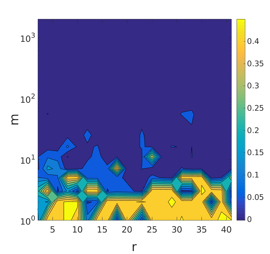
In the first experiment we studied the influence of $r$ and $m$ on the prediction accuracy of PAC-Bayesian aggregation. We considered 20 values of $m$ in $[1,n]$ and 20 values of $r$ in $[2,d+1]$. For each pair of $m$ and $r$ the prediction accuracy of PAC-Bayesian aggregation was evaluated, resulting in a matrix of losses. To simplify the comparison we subtracted the prediction accuracy of the baseline, thus zero values correspond to matching the accuracy of the baseline. In Figure 1 we show a heatmap of this matrix for two UCI datasets and the results for the remaining datasets are provided in Appendix D.1. Overall, reasonably small values of $m$ and $r$ were sufficient for matching the accuracy of SVM tuned by cross-validation.

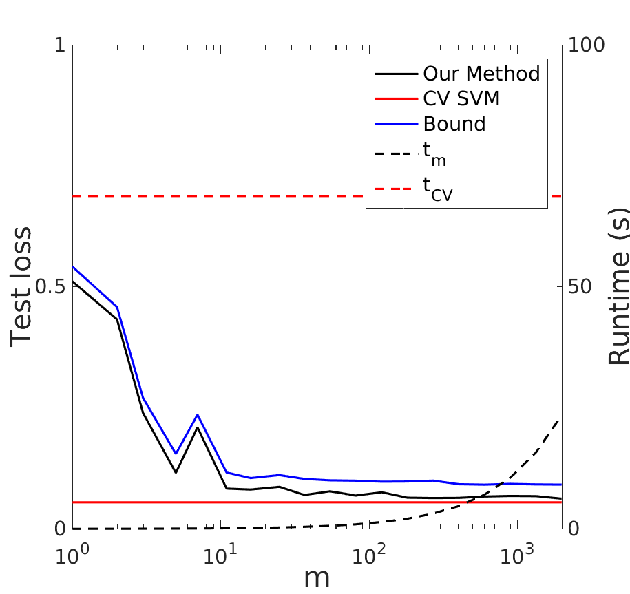
In the second experiment we provide a closer look at the effect of increasing the number $m$ of weak SVMs when their training set sizes $r$ are kept fixed. We picked $r=d+1$ and ran our training procedure with 20 values of $m$ in $[1,n]$. In Figure 2 we present the prediction accuracy of the resulting weighted majority vote vs. prediction accuracy of the baseline for four datasets. The graphs for the remaining datasets are provided in Appendix D.1. We also show the running time of our procedure vs. the baseline. The running time of the baseline includes cross-validation and training of the final SVM on the whole training set, while the running time of PAC-Bayesian aggregation includes training of $m$ weak SVMs, their validation, and the computation of $\rho$. In addition, we report the value of PAC-Bayes-kl bound from Theorem 2 on the expected loss of the randomized classifier defined by $\rho$. The kl divergence was inverted numerically to obtain a bound on the expected loss $\mathbb{E}_{\rho}\left[L(h)\right]$. The bound was adapted to our construction by replacing $n$ with $n-r$ and $\mathbb{E}_{\rho}\left[\hat{L}(h,S)\right]$ with $\mathbb{E}_{\rho}\left[\hat{L}^{\text{val}}(h,S)\right]$. We note that since the bound holds for any posterior distribution, it also holds for the distribution found by minimization of the bound in Theorem 13. However, since Theorem 13 is a relaxation of PAC-Bayes-kl bound, using PAC-Bayes-kl for the final error estimate is slightly tighter. The bound on the loss of $\rho$-weighted majority vote is at most a factor of 2 larger than than the bound for the randomized classifier. In calculation of the bound we used $\delta=0.05$. We conclude from the figure that relatively small values of $m$ are sufficient for matching or almost matching the prediction accuracy of the baseline, while the run time is reduced dramatically. We also note that the bound is exceptionally tight.

In our last experiment we tested quasiconvexity of ${\cal F}(\lambda)$. Theorem 5 provided theoretical guarantee of quasiconvexity for small $m$ and numerical evaluation has further shown that ${\cal F}(\lambda)$ was convex for all values of $m$ used in our experiments. For testing the theoretical guarantees we increased $m$ in steps of 10 until the sufficient condition for strong quasiconvexity in Theorem 5 was violated. The condition included adjustment of interval boundaries $a$ and $b$, as described in Appendix B.1, and improved value of $b$, as described in Appendix B.2. The experiments were repeated 10 times for each dataset, where in each experiment the training sets were redrawn and a new set of hypotheses was trained, leading to a new set of validation losses $\hat{L}^{\text{val}}$. In Table 2 we report the average over the 10 repetitions of the maximal values of $m$ with guaranteed quasiconvexity. Since ${\cal F}(\lambda)$ is always quasiconvex for $m\leq K(0,0)+1$, where $K(0,0)=\frac{e^{2}}{4}\ln\frac{4n}{\delta^{2}}$ (see equation (15) in Appendix B.1), we report the value of $K(0,0)+1$ whenever it was not possible to ensure quasiconvexity with larger $m$. When it was not possible to guarantee quasicovexity theoretically we tested the shape of ${\cal F}(\lambda)$ empirically. Figure 3 shows a few typical examples. The plots in Figure 3 were constructed in the following way: given a sample $S$, we trained $m$ weak SVMs. We then computed the corresponding vector of validation losses, $\hat{L}^{\text{val}}(h,S)$. For each value in a grid of $\lambda$-s, we computed the corresponding $\rho$ according to equation (7). Finally, we substituted the value of $\rho_{\lambda}$ and $\lambda$ into equation (3) to get the value of the bound. In all our calculations we used a uniform prior and $\delta=0.05$. The figure shows that ${\cal F}(\lambda)$ was convex in $\lambda$ in all the cases.

We have presented a new PAC-Bayesian inequality, an alternating procedure for its minimization, and a way to construct a finite hypothesis space for which the bound and minimization procedure work particularly well. We have derived sufficient conditions for the minimization procedure to converge to the global optimum of the bound. We have shown that the procedure is competitive with cross-validation in tuning the trade-off between complexity and empirical performance of $\rho$. In addition, it provides tight high-probability generalization guarantees and achieves prediction accuracies on par with kernel SVMs tuned by cross-validation, but at a considerably lower computation cost.

In our experiments the bound turned to be convex even when the sufficient conditions of Theorem 5 were violated. It suggests that further relaxation of these conditions may be possible to achieve in future work.