Hitting statistics from quantum jumps

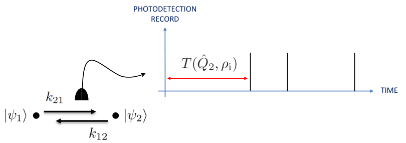
The quantum-jump approach to dissipative quantum dynamics has traditionally been used for efficiently solving master equations [14, 15, 16, 17], or calculating photon statistics in photon counting [18, 19]. It also goes by the name of Monte Carlo wavefunctions or quantum trajectories due to the different contexts in which it was invented (although quantum jumps correspond only to a subset of unravellings within quantum-trajectory theory¹¹ 1 We have devoted a separate discussion to the use of other unravellings in hitting problems in Sec. 7.2. If the reader is already familiar with quantum-trajectory theory then this may be read now, but otherwise should be left till the end for the nonexperts.). We refer the reader to Ref. [20] for a comprehensive review of how the quantum-jump method was developed. Figure 1 illustrates a typical scenario where quantum jumps are applied e.g. Refs. [21, 22, 23, 24]. There is usually a system (described by a master equation [25]), say a lossy cavity or a two-level atom which dissipates energy into the environment in the form of photons. The emitted photons are then measured by a photodetector. Each count, or photodetector “click” appears as a spike in the photodetection record. The quantum-jump formalism then allows one to compute the system evolution conditioned on a given photodetection record where each detector click is associated with a “jump” in the system Hilbert space. Periods of no clicks then correspond to system evolution with no jumps. The quantum-jump method states that an average over a large number of such conditioned states will reproduce the solution to the master equation. Thus in solving the master equation, one also gains access to the statistics of photon arrival times at the detector. Photon statistics are therefore often calculated using the quantum-jump method [24, 26, 27]. In fact, Carmichael derived the quantum-jump method [18, 19] from the photon-counting distribution due to Kelley and Kleiner [28]. It is this intuition between photodetector clicks and quantum jumps that we will exploit for deriving the hitting-time statistics in quantum walks. To see this we need to first explain what hitting times are: In quantum-walk theory the system, usually called the walker, has a Hilbert space spanned by a countable set of orthonormal states $\{|{\psi_{n}}\rangle\}_{n}$, called sites, nodes, or vertices. The hitting time is defined as the time required for the walker to reach (or “hit”) some “final” state $|{\psi_{N}}\rangle$ for the first time given that initially it was at $|{\psi_{m}}\rangle$. The hitting time is a random variable since the first time that the walker arrives at $|{\psi_{N}}\rangle$ will vary from one realisation of the quantum walk to another. It therefore makes sense to speak of the average hitting time and its higher-order statistics. We will often call the hitting-time distribution simply as the hitting distribution for ease of reference. Similarly, hitting statistics (as in the title) refers to the statistics of hitting times. It should be noted that the problem we have defined here has an analogue in classical Markov chains, where the orthonormal set $\{|{\psi_{n}}\rangle\}_{n}$ is replaced by a set of probabilities. The temporal evolution of the classical walker is then governed by a set of rate equations for the site probabilities [29] which plays the role of the master equation in the quantum case. In fact, one of the quantum-walk models that we will discuss two paragraphs down is based on this idea. We should also mention that hitting times are usually called first-passage times in the classical theory of Markov chains and most areas of science where this concept appears, see e.g. Refs. [30, 31, 32].

The quantum-jump method lends itself naturally to a hitting problem because the question one is asking, starting from the initial time, is whether the system has made a transition to the final state or not. This leads to a very natural division of the system evolution into two types—either a transition to the final state occurred, or it has not, and this corresponds to a system evolution conditioned on “jumps” and “no jumps”. We illustrate this idea on an arbitrarily chosen quantum walk in Fig. 2. The walker can move between any two vertices connected by a line, usually called an edge (edges and vertices together form a graph as shown). We are not defining the edges precisely for the moment but one may think of each edge as given by a completely-positive trace-preserving map, i.e. a Kraus channel of some sort [1, 33]. Consider the hitting problem defined by the initial and final states shown as $|{\psi_{1}}\rangle$ and $|{\psi_{N}}\rangle$ respectively on the graph. Imagine now that each transition on the graph emits a photon. Then we can find out when the quantum walker will arrive at $|{\psi_{N}}\rangle$ by associating photodetectors with the edges connected to $|{\psi_{N}}\rangle$ (assuming our photodetectors only measure photons emitted from transitions to $|{\psi_{N}}\rangle$). If we superimpose the photodetection records from these detectors then we will observe an overall record shown on the right of Fig. 2. In this case a photodetector click signifies that our walker is at $|{\psi_{N}}\rangle$, and the first such click provides the hitting time. We will not be able to distinguish which channel the quantum walker took to reach $|{\psi_{N}}\rangle$ but this does not matter if we only care about when the walker visits $|{\psi_{N}}\rangle$. This analogy makes clear how the quantum-jump method can be applied to calculate the distribution of hitting times in quantum walks. The theory of quantum walks is more than two decades old so let us briefly review some of the key developments in this field and then discuss where our work stands in relation to the literature on this topic.

The concept of a quantum walk was first introduced by Aharonov and coworkers in 1993 [34]. Quantum walks can be categorised into one of two classes—either a walk in discrete time, or a walk in continuous time [35]. Quantum walks in discrete time follow the idea originally prosposed by Aharonov and colleagues where a quantum coin is introduced. Classically, a random walk on a line involves a coin toss, the result of which determines whether the walker moves one step to the left, or one step to the right. In the quantum version the coin is simply a two-state system. The movement of the walker is then effected by a (quantum) coin toss implemented as a Hadamard gate $\hat{C}$, followed by applying a shift operator $\hat{S}$ to change the walker’s position conditioned on the coin state [36]. Each application of the unitary operator $\hat{U}\equiv\hat{S}\hat{C}$ then evolves the walker in one time step. For a unitary quantum walk, the notion of hitting becomes fuzzy due to the walker’s ability to be in a superposition of sites. As a result, multiple definitions of hitting have been proposed [37, 38]. Among these, the definition of hitting based on repeated measurements proposed by Krovi and Brun in Ref. [38] will be useful for our analysis. Applications of discrete-time quantum walks include the design of search algorithms [39, 40], and implementing universal quantum computation [41]. Continuous-time quantum walks on the other hand do not use a coin. Instead, the quantum walker evolves according to a unitary operator generated by a Hamiltonian, i.e. $\hat{U}(t)=\exp(-i\hat{H}t)$ with $\hat{H}$ parametrised by hopping rates to adjacent nodes. Quantum walks in continuous time were first introduced by Farhi and Gutmann [42] in close analogy to continuous-time Markov chains [42, 43]. Their hitting properties were then studied by Varbanov and colleagues [44] who defined hitting times through jumplike weak measurements. The quantum-jump treatment in the present paper can also be seen as a weak measurement of the walker position in that most of the time one gets a null result (no jumps) which does not modify the walker state very much but once in a while a collapse (a jump) happens which changes the walker state drastically [45]. As with the discrete-time case, continuous-time quantum walks have also been shown to give rise to exponential speedups over classical algorithms for searching [46] and solving black-box problems [47]. It has also been shown that universal quantum computation can be achieved using continuous-time quantum walks [48]. Discrete-time quantum walks were then generalised to allow for non-unitary evolution. These are known as open quantum walks and were first introduced by Attal and collaborators [49, 50]. Here the coin changes its state according to a completely-positive trace-preserving map and the evolution operator $\hat{U}$ for the unitary walk is also replaced by a completely-positive trace-preserving map. A continuous-time model was subsequently proposed by Pellegrini as the continuous-time limit of the discrete-time open quantum walk [51]. Most recently, Liu and Balu proposed yet another continuous-time model of open quantum walks by starting with a master equation in the Lindblad form [52]. This approach to defining quantum walks is in the same spirit as Farhi and Gutmann’s for unitary walks as already alluded to above. They (Farhi and Gutmann) viewed the Schrödinger equation as the analogue of the rate equation for probabilities in classical Markov chains. Generalising this to allow for non-unitary dynamics naturally leads to a master equation. We also consider here continuous-time open quantum walks described by a master equation.

Of particular interest for our work is the application of quantum trajectories in Refs. [49, 50, 51]. These works were motivated by the fact that quantum trajectories offer an efficient means of simulating quantum walks and have the advantage of providing a visualisation of the walk. Lardizabal and Souza have recently defined hitting times using quantum trajectories [53], but for the discrete-time model due to Attal and colleagues [49, 50]. Given that quantum trajectories were invented in the context of Lindblad-form master equations the latter is in fact the most natural setting in which to consider them. For such non-unitary graphs one can therefore bypass the formalism of positive operator-valued measures (as in Ref. [44] for example) and give a quantum-trajectory treatment of the hitting problem. Our aim in this paper is to define the hitting time for open quantum walks as the time for the first jump to occur and use this as the basis for calculating the distribution of hitting times and its statistical moments. Our result also corrects Ref. [54] which claims to have calculated the average hitting time for continuous-time open quantum walks. However, an inspection of Ref. [54] shows their model to be purely classical. A summary of the relevant literature is given in Fig. 3.

Here we will explain the method of quantum jumps as illustrated in Fig. 1, i.e. in the context of photon counting. This makes the basic structure of the formalism intuitive. Assume for simplicity that the system in Fig. 1 is a single-mode field in an optical cavity with one slightly lossy mirror. The lossy mirror allows the single-mode light to couple to the field outside the cavity which we assume is in a vacuum state. This is described by a master equation which has only one dissipative channel, given by

$\displaystyle\dot{\rho}(t)={\cal L}\rho(t)\equiv-i\big[\hat{H},\rho(t)\big]+\hat{c}\,\rho(t)\,\hat{c}^{\dagger}-\frac{1}{2}\,\big\{\hat{c}^{\dagger}\hat{c},\rho(t)\big\}\;,$

(1)

where $\hat{c}=\sqrt{\gamma}\,\hat{a}$ with $\gamma$ being a damping coefficient and $\hat{a}$ a bosonic annihilation operator. We are using the notation $\{\hat{A},\hat{B}\}$ for the anticommutator of any two operators $\hat{A}$ and $\hat{B}$. The terms containing $\hat{c}$ modify the usual unitary dynamics (which conserves the system’s energy) to include a dissipative process (here being the loss of photons to the vacuum outside the optical cavity). The quantum-jump formalism provides a way to understand these terms as follows. The system state $\rho(t)$ can evolve over an infinitesimal time interval $dt$ conditioned on two types of detection events—a count, and no count (Fig. 1). Given an initial state $\rho(t)$, the probability of registering a count in the interval $[t,t+dt)$ is given by

$\displaystyle\wp_{1}(dt)={\rm Tr}\big\{{\cal J}\rho(t)\big\}dt={\rm Tr}\big\{\hat{c}^{\dagger}\hat{c}\,\rho(t)\big\}dt\;,$

(2)

where we have defined

$\displaystyle{\cal J}\rho\equiv\hat{c}\,\rho\,\hat{c}^{\dagger}\;.$

(3)

Here we are assuming our detector in Fig. 1 is ideal. The state change conditioned on observing a count (a spike in the photodetection record in Fig. 1) is effected by

$\displaystyle\rho_{1}(t+dt)=\frac{{\cal J}\rho(t)}{{\rm Tr}\big\{{\cal J}\rho(t)\big\}}\;.$

(4)

Equation (4) is called a quantum jump and $\hat{c}$ is referred to as a jump operator. A quantum jump causes $\rho(t)$ to change discontinuously in time.

The second type of evolution is conditioned on the event that no counts were registered in $[t,t+dt)$. This is commonly referred to as the no-jump evolution and occurs with probability

$\displaystyle\wp_{0}(dt)=1-\wp_{1}(dt)\;.$

(5)

The state at time $t+dt$ conditioned on a no-count observation is

$\displaystyle\rho_{0}(t+dt)=\frac{e^{\bar{\cal L}dt}\rho(t)}{{\rm Tr}\big[e^{\bar{\cal L}dt}\rho(t)\big]}\;,$

(6)

where

$\displaystyle\bar{\cal L}\,\rho(t)\equiv-i\big[\hat{H},\rho(t)\big]-\frac{1}{2}\,\big\{\hat{c}^{\dagger}\hat{c},\rho(t)\big\}\;.$

(7)

Note that $\wp_{0}(dt)$ can be written explicitly in terms of (7) as

$\displaystyle\wp_{0}(dt)={\rm Tr}\big[e^{\bar{\cal L}dt}\rho(t)\big]\;.$

(8)

It helps to consider two generalisations of the basic structure given by (2)–(7) for the application of quantum jumps to quantum walks coming up later.

We now define the problem to which we would like to apply the quantum-jump formalism. Our problem can be set up in analogous fashion to a classical Markov chain problem in continuous time. We are given a quantum system that makes transitions between a set of discrete states

$\displaystyle\mathbb{S}_{N}\equiv\{|{\psi_{1}}\rangle,|{\psi_{2}}\rangle,\ldots,|{\psi_{N}}\rangle\}\;.$

(18)

The set $\mathbb{S}_{N}$ forms an orthonormal basis for the system. The space in which the system resides is thus spanned by $\mathbb{S}_{N}$. In the language of quantum-walk theory, each state in $\mathbb{S}_{N}$ is referred to as a vertex and the system is referred to as a quantum walker. We shall also refer to the elements of $\mathbb{S}_{N}$ as states, or sites.

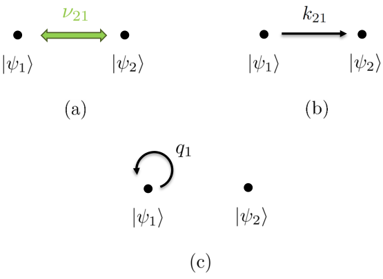
We must therefore also define the exact manner in which the system makes transitions between different states (analogous to specifying a transtion matrix in classical Markov chains). We assume that our system is undergoing dynamics that can be composed from three basic processes. They are coherent transitions, incoherent population transfer, and dephasing. These processes are represented schematically in Fig. 4 for two vertices and are explained below.

We now derive a closed-form expression for the hitting time distribution on an arbitrary graph using quantum-jump formalism. For simplicity we first consider a graph where there are no loops, i.e. no dephasing:

$\displaystyle\frac{d}{dt}\,\rho(t)={\cal L}\,\rho(t)\equiv-\frac{i}{2}\,\underset{m\neq n}{\sum_{m=1}^{N-1}\sum_{n=1}^{N-1}}\,\big[\hat{H}_{mn},\rho(t)\big]+\underset{m\neq n}{\sum_{m=1}^{N}\sum_{n=1}^{N}}\,k_{mn}\,{\cal D}_{mn}\,\rho(t)\;.$

(36)

Note that we have divided the sum over commutators by half to compensate for double counting. This is because $\hat{H}_{mn}=\hat{H}_{nm}$. In general not every state will be connected to every other state via all possible processes. When this is the case we can simply choose which processes to switch off in (36) by setting the relevant rates zero. One may have also noticed that the sums over the coherent transitions (the commutator terms) do not include transitions to the final state $|{\psi_{N}}\rangle$. This is because only the incoherent transitions to $|{\psi_{N}}\rangle$ are detectable in the quantum-jump formalism. Later on (in Sec. 6) we will show how the hitting probability density can be obtained when there are coherent transitions to $|{\psi_{N}}\rangle$ by introducing an artifical dissipative channel.

In order to apply the quantum-jump technique we first note that (34) can also be rewritten using Bayes’s rule as

	$\displaystyle h(t)\,dt={}$	$\displaystyle{\rm Pr}\Big\{\rho(\tau)=\hat{Q}_{N}\;\text{for}\;\tau\in[t,t+dt)\;\Big|\;\rho(\tau)\neq\hat{Q}_{N}\;\text{for}\;\tau\in(0,t)\,,\,\rho(0)=\rho_{\rm i}\Big\}$
		$\displaystyle\times{\rm Pr}\Big\{\rho(\tau)\neq\hat{Q}_{N}\;\text{for}\;\tau\in(0,t)\;\Big|\;\rho(0)=\rho_{\rm i}\Big\}\;.$		(37)

Each factor on the right-hand side in (37) can now be calculated using the prescription laid out in Sec. 2.1. To do this we map (13) directly to (36) by making the following identification

	$$\displaystyle\big\{\hat{c}_{q}\big\}_{q}=\big\{\sqrt{k_{mn}}\,\hat{Q}_{mn}\big\}_{m,n}\;,$$		(38)
	$$\displaystyle\hat{H}=\frac{1}{2}\,\underset{m\neq n}{\sum_{m=1}^{N-1}\sum_{n=1}^{N-1}}\,\hat{H}_{mn}\;.$$		(39)

In terms of the multichannel theory of quantum jumps in Sec. 2.1.2, each channel is now labelled by an ordered pair $(m,n)$ where $m=1,2,\ldots N$, and $n=1,2,\ldots N$, and a quantum jump is simply the detection of a transition between any two nodes, say $|{\psi_{m}}\rangle$ and $|{\psi_{n}}\rangle$. The measurement efficiency for this quantum jump can then be labelled by $\eta_{mn}$, and is a number which corresponds to the fraction of jumps observed in the $|{\psi_{n}}\rangle\to|{\psi_{m}}\rangle$ incoherent transition. The actual number of jumps from $|{\psi_{n}}\rangle$ to $|{\psi_{m}}\rangle$ will always be greater than the observed number of jumps unless $\eta_{mn}=1$. We can then express the probability of finding the system in the final state $|{\psi_{N}}\rangle$ using the probability of detecting a jump to $|{\psi_{N}}\rangle$ provided that all transitions to $|{\psi_{N}}\rangle$ are monitored with unit efficiency. This identification then dictates how we should set $\eta_{mn}$ for all $m$ and $n$, namely that $\eta_{Nn}=1$ for any $n$. Transitions to states other than $|{\psi_{N}}\rangle$ are irrelevant so we simply do not monitor these transitions. Therefore we set $\eta_{mn}=0$ for every $m\neq N$. We must use this set of detection efficiencies in the formalism outlined in Sec. 2.1.2 in order for it to be applicable for hitting-time calculations. This prompts us to assign a special label, $\bm{\eta}_{\star}$, for the detection efficiencies to be used:

$\displaystyle\bm{\eta}_{\star}\,\Longleftrightarrow\,\eta_{mn}=\delta_{mN}\;.$

(40)

The jump superoperator (14) on using (38) and (40), becomes

$\displaystyle{\cal J}({\bm{\eta}}_{\star})\,\rho\equiv\sum_{n=1}^{N-1}\,k_{Nn}\,\hat{Q}_{Nn}\,\rho\;\hat{Q}^{\dagger}_{Nn}\;.$

(41)

An application of ${\cal J}({\bm{\eta}}_{\star})$ effects an instantaneous collapse of the system to the state $|{\psi_{N}}\rangle$. From (15) and (38), the probability of detecting a jump in time $dt$ given $\rho(t)$ is thus

$\displaystyle\wp_{1}(\bm{\eta}_{\star};dt)={\rm Tr}\big[{\cal J}(\bm{\eta}_{\star})\,\rho(t)\big]\,dt=\sum_{n=1}^{N-1}\;k_{Nn}\,\langle{\psi_{n}}|\rho(t)|{\psi_{n}}\rangle\,dt\;.$

(42)

If $\rho(t)$ in (42) is a state where no transitions to $|{\psi_{N}}\rangle$ are observed in the time interval $[0,t)$ given some initial state $\rho(0)$, then (42) is exactly the first factor on the right-hand side of (37). Such a state can be directly obtained by solving the no-jump evolution defined by (16), (38), and (39):

	$\displaystyle\frac{d}{dt}\,\bar{\rho}(t)\equiv\bar{\cal L}(\bm{\eta}_{\star})\,\bar{\rho}(t)={}$	$\displaystyle-\frac{i}{2}\,\underset{m\neq n}{\sum_{m=1}^{N-1}\sum_{n=1}^{N-1}}\,\big[\hat{H}_{mn},\bar{\rho}(t)\big]+\underset{m\neq n}{\sum_{m=1}^{N}\sum_{n=1}^{N}}\;k_{mn}\,(1-\delta_{mN})\,\hat{Q}_{mn}\,\bar{\rho}(t)\,\hat{Q}^{\dagger}_{mn}$
		$\displaystyle-\frac{1}{2}\,\underset{m\neq n}{\sum_{m=1}^{N}\sum_{n=1}^{N}}\;k_{mn}\,\big\{\hat{Q}^{\dagger}_{mn}\hat{Q}_{mn},\bar{\rho}(t)\big\}\;.$		(43)

It helps to rewrite $\bar{\cal L}(\bm{\eta}_{\star})\;\!\bar{\rho}(t)$ so that its meaning is more obvious. Expanding the sum containing $(1-\delta_{mN})$ we get

	$\displaystyle\bar{\cal L}(\bm{\eta}_{\star})\,\bar{\rho}(t)={}$	$\displaystyle-\frac{i}{2}\,\underset{m\neq n}{\sum_{m=1}^{N-1}\sum_{n=1}^{N-1}}\,\big[\hat{H}_{mn},\bar{\rho}(t)\big]+\underset{m\neq n}{\sum_{m=1}^{N}\sum_{n=1}^{N}}\;k_{mn}\,\hat{Q}_{mn}\,\bar{\rho}(t)\,\hat{Q}^{\dagger}_{mn}$
		$\displaystyle-{\cal J}({\bm{\eta}}_{\star})\,\bar{\rho}(t)-\frac{1}{2}\,\underset{m\neq n}{\sum_{m=1}^{N}\sum_{n=1}^{N}}\;k_{mn}\,\big\{\hat{Q}^{\dagger}_{mn}\hat{Q}_{mn},\bar{\rho}(t)\big\}\;.$		(44)

It is simple to see that

$\displaystyle\underset{m\neq n}{\sum_{m=1}^{N}\sum_{n=1}^{N}}\;k_{mn}\,\hat{Q}_{mn}\,\bar{\rho}(t)\,\hat{Q}^{\dagger}_{mn}={\cal J}({\bm{\eta}}_{\star})\,\bar{\rho}(t)+\underset{m\neq n}{\sum_{m=1}^{N-1}\sum_{n=1}^{N}}\;k_{mn}\,\hat{Q}_{mn}\,\bar{\rho}(t)\,\hat{Q}^{\dagger}_{mn}\;,$

(45)

and similarly

$\displaystyle\underset{m\neq n}{\sum_{m=1}^{N}\sum_{n=1}^{N}}\;k_{mn}\,\big\{\hat{Q}^{\dagger}_{mn}\hat{Q}_{mn},\bar{\rho}(t)\big\}=\sum_{n=1}^{N-1}\;k_{Nn}\,\big\{\hat{Q}^{\dagger}_{Nn}\hat{Q}_{Nn},\bar{\rho}(t)\big\}+\underset{m\neq n}{\sum_{m=1}^{N-1}\sum_{n=1}^{N}}\;k_{mn}\,\big\{\hat{Q}^{\dagger}_{mn}\hat{Q}_{mn},\bar{\rho}(t)\big\}\;.$

(46)

Substituting (45) and (46) into (44) gives

$\displaystyle\bar{\cal L}(\bm{\eta}_{\star})\,\bar{\rho}(t)={}$

$\displaystyle-\frac{i}{2}\,\underset{m\neq n}{\sum_{m=1}^{N-1}\sum_{n=1}^{N-1}}\,\big[\hat{H}_{mn},\bar{\rho}(t)\big]+\underset{m\neq n}{\sum_{m=1}^{N-1}\sum_{n=1}^{N}}\;k_{mn}\,{\cal D}_{mn}\,\bar{\rho}(t)+\sum_{n=1}^{N-1}\;k_{Nn}\,\bar{{\cal D}}_{Nn}\,\bar{\rho}(t)\;,$

(47)

where we have defined

$\displaystyle\bar{{\cal D}}_{Nn}\,\rho=-\frac{1}{2}\,\big\{\hat{Q}^{\dagger}_{Nn}\hat{Q}_{Nn},\rho\big\}\;.$

(48)

As already described at the outset, the first term in (47) describes coherent population transfer between states other than the final state $|{\psi_{N}}\rangle$ (recall Sec. 2.2.1). The second term in (47) describes incoherent transitions that either move populations out of $|{\psi_{N}}\rangle$, or between any two states except for $|{\psi_{N}}\rangle$ (see Sec. 2.2.2). The last term in (47) is similar in form to ${\cal D}_{mn}$ except that terms of the form $\hat{Q}_{Nn}\,\bar{\rho}(t)\,\hat{Q}^{\dagger}_{Nn}$ have been removed. But these are the terms which describe jumps to the final state. Therefore $\bar{{\cal D}}_{Nn}$ is a superoperator which describes how the system evolves conditioned on no jumps to $|{\psi_{N}}\rangle$. Substituting the formal solution of (43) into (42) we thus obtain

		$\displaystyle{\rm Pr}\Big\{\rho(\tau)=\hat{Q}_{N}\;\text{for}\;\tau\in[t,t+dt)\;\Big|\;\rho(\tau)\neq\hat{Q}_{N}\;\text{for}\;\tau\in(0,t)\,,\,\rho(0)=\rho_{\rm i}\Big\}$
		$\displaystyle=\sum_{n=1}^{N}\;k_{Nn}\,\frac{\langle{\psi_{n}}|\;\!e^{\bar{{\cal L}}(\bm{\eta}_{\star})\,t}\rho_{\rm i}\;\!|{\psi_{n}}\rangle}{{\rm Tr}\big[e^{\bar{{\cal L}}(\bm{\eta}_{\star})\,t}\rho_{\rm i}\big]}\;dt\;.$		(49)

Note that (43) produces a trace-decreasing state, which is why we have used an overbar for the density operator and the generator of time evolution. Following Sec. 2.1.2 we see that the norm of $\bar{\rho}(t)$ is precisely the probability of no jumps in the interval $[0,t)$, given some initial state i.e.

$\displaystyle{\rm Pr}\Big\{\rho(\tau)\neq\hat{Q}_{N}\;\text{for}\;\tau\in[0,t)\;\Big|\;\rho(0)=\rho_{\rm i}\Big\}={\rm Tr}\big[e^{\bar{{\cal L}}(\bm{\eta}_{\star})\,t}\rho_{\rm i}\;\!\big]\;.$

(50)

The product of (49) and (50) simply cancels the norm of $\bar{\rho}(t)$ giving the final expression for the hitting probability density as

$\displaystyle h\big(t;\hat{Q}_{N},\rho_{\rm i}\big)=\sum_{n=1}^{N-1}\;k_{Nn}\,\langle{\psi_{n}}|\,e^{\bar{{\cal L}}(\bm{\eta}_{\star})\,t}\,\rho_{\rm i}\;\!|{\psi_{n}}\rangle\;.$

(51)

This completes our derivation of the hitting distribution using the quantum-jump method.

We now illustrate (51) with a simple example. Consider the graph shown in Fig. 5(a). This is an example with $N=4$ so by our convention the final state is $\rho_{\rm f}=\left|{\psi_{4}}\rangle\langle{\psi_{4}}\right|$. We will let the initial state be $\rho_{\rm i}=\left|{\psi_{1}}\rangle\langle{\psi_{1}}\right|$. In Fig. 5(b), (c), and (d), we plot the hitting distribution for various amounts of coherence between states $|{\psi_{1}}\rangle$ and $|{\psi_{2}}\rangle$ while keeping other parameters constant (see figure caption for their values). We observe that as $\Omega_{21}$ is increased from 5 [Fig. 5(b)] to 50 [Fig. 5(d)], the hitting distribution starts to show more and more oscillations due to the increased level of coherence. Classically, only incoherent transitions are permitted so hitting distributions do not exhibit oscillations. We can see from Fig. 5(b) that for $\Omega_{21}=5$ the oscillations in the hitting distribution are dying out and the quantum walk is in transition to the classical regime. Furthermore, the oscillations in the hitting distribution can actually reach zero (or near zero) at its minimum meaning that there are times at which it is impossible to find the walker at $|{\psi_{4}}\rangle$. Again, such features would not appear in a purely classical walk since incoherent transitions cannot produce any interference effects. For variation we show in Fig. 6 what happens when we change $\Omega_{32}$ instead of $\Omega_{21}$ while keeping every other parameter constant (see the figure caption for the actual values). Like Fig. 5, the amount of oscillations increases as $\Omega_{32}$ is increased, but now this is accompanied by a lengthening of the tail of the hitting distribution. The shape of the hitting distribution depends on the exact manner in which the probability amplitudes for the different paths of the quantum walk interfere. A comparison of Fig. 5 with Fig. 6 illustrates that hitting times of a given graph can be much more sensitive to one coherent transition but not others. We will have more to say about this in Sec. 4.

We obtained (51) based on (36) which does not have the dephasing processes defined in (30). The omission of dephasing connections was simply to make the derivation easier to follow. If we include dephasing in ${\cal L}$ then the dephasing terms will simply carry through to $\bar{{\cal L}}(\bm{\eta}_{\star})$. The expression for the hitting-time probability density will still be given by (51), just with an $\bar{{\cal L}}(\bm{\eta}_{\star})$ that includes dephasing connections. Stated more formally, we can consider a graph defined by

$\displaystyle\frac{d}{dt}\,\rho(t)={\cal L}\,\rho(t)\equiv-\frac{i}{2}\,\underset{m\neq n}{\sum_{m=1}^{N-1}\sum_{n=1}^{N-1}}\,\big[\hat{H}_{mn},\rho(t)\big]+\underset{m\neq n}{\sum_{m=1}^{N}\sum_{n=1}^{N}}\;k_{mn}\,{\cal D}_{mn}\,\rho(t)+\sum_{n=1}^{N}\;q_{n}\,{\cal D}_{n}\,\rho(t)\;.$

(52)

Note that the total number of incoherent channels in this case is given by $L=N^{2}$ and we can make the following identification for the Lindblad operators in (13):

$$\displaystyle\big\{\hat{c}_{q}\big\}_{q=1}^{N^{2}-N}=\big\{\sqrt{k_{mn}}\,\,\hat{Q}_{mn}\big\}_{m,n}\;,\quad\big\{\hat{c}_{q}\big\}_{q=N^{2}-N+1}^{N^{2}}=\big\{\sqrt{q_{n}}\,\,\hat{Q}_{n}\big\}_{n}\;.$$

(53)

The Hamiltonian in (13) is still given by (39). The detection efficiencies should now be set according to

$\displaystyle\bm{\eta}_{\star}\,\Longleftrightarrow\,\eta_{mn}=\delta_{mN}\;,\quad n=1,2,\ldots,L/2\;.$

(54)

This then gives

	$\displaystyle\bar{\cal L}(\bm{\eta}_{\star})\,\bar{\rho}(t)={}$	$\displaystyle-\frac{i}{2}\,\underset{m\neq n}{\sum_{m=1}^{N-1}\sum_{n=1}^{N-1}}\,\big[\hat{H}_{mn},\bar{\rho}(t)\big]+\sum_{n=1}^{N}\;q_{n}\,{\cal D}_{n}\,\bar{\rho}(t)$
		$\displaystyle+\underset{m\neq n}{\sum_{m=1}^{N-1}\sum_{n=1}^{N}}\;k_{mn}\,{\cal D}_{mn}\,\bar{\rho}(t)+\sum_{n=1}^{N-1}\;k_{Nn}\,\bar{{\cal D}}_{Nn}\,\bar{\rho}(t)\;.$		(55)

Replacing $\bar{{\cal L}}(\bm{\eta}_{\star})$ in (51) with (55) then gives the distribution of hitting times for the general graph.

The reason why adding dephasing connections to the graph does not change the form of hitting distribution as a function of $\bar{{\cal L}}(\bm{\eta}_{\star})$ is because the quantum-jump method works by detecting transitions to the final state $|{\psi_{N}}\rangle$. Of the three types of connections that we consider, only two can induce transitions between states—coherent and incoherent population transfer. The third type, i.e dephasing, changes only the coherences in the system. Of course changing coherences in the graph does affect how quickly the final state is reached. That is to say, the distribution of hitting times for a state diagram with dephasing will be a different function of $t$ compared to one without dephasing but otherwise identical in all respects.

For illustration we include in Fig. 7 hitting distributions for the graph with dephasing of $|{\psi_{2}}\rangle$, see Fig. 7(a). The plots in Fig. 7 are identical to Fig. 5(d) except with various amounts of dephasing added as indicated in the plots. Here the dephasing rate is $q_{2}$ and as we increase this rate the quantum walk becomes more classical. This can be seen in passing from Fig. 7(b) to (d) where the oscillations which we attributed to the quantum-mechanical nature of the walk in Fig. 5 gradually die out. This is to be expected since by increasing $q_{2}$ we are making the walk more classical, in other words, making it more and more difficult to share coherences between $|{\psi_{2}}\rangle$ and other nodes in the graph. Next we calculate the moments of $h\big(t;\hat{Q}_{N},\rho_{\rm i}\big)$.

The $n$th raw statistical moment of the hitting time $T(\hat{Q}_{N},\rho_{\rm i})$ is defined as

$\displaystyle{\rm E}\big[T^{n}(\hat{Q}_{N},\rho_{\rm i})\big]=\int_{0}^{\infty}dt\;t^{n}\;h(t;\hat{Q}_{N},\rho_{\rm i})\;,$

(56)

where we are using the notation ${\rm E}[X]$ to mean the ensemble average of an arbitrary random variable $X$. Although having the hitting-time distribution is formally equivalent to knowing the statistics of $T(\hat{Q}_{N},\rho_{\rm i})$, deriving a closed-form expression for (56) is still a nontrivial task. We will show in Sec. 4.2 that (56) evaluates to

$\displaystyle{\rm E}\big[T^{n}(\hat{Q}_{N},\rho_{\rm i})\big]=(-1)^{n+1}\,n!\sum_{m=1}^{N-1}\,k_{Nm}\,\langle{\psi_{m}}|\,\bar{{\cal L}}_{\star}^{+}{}^{(n+1)}\,\rho_{\rm i}\;\!|{\psi_{m}}\rangle$

(57)

where we have defined the shorthand

$\displaystyle\bar{{\cal L}}_{\star}=\bar{\cal L}(\bm{\eta}_{\star})\;,$

(58)

and $\bar{{\cal L}}_{\star}^{+}$ is the Moore–Penrose pseudoinverse of $\bar{{\cal L}}_{\star}$, defined by

$\displaystyle\bar{{\cal L}}_{\star}^{+}\,\bar{{\cal L}}_{\star}\,\bar{{\cal L}}_{\star}^{+}=\bar{{\cal L}}_{\star}^{+}\;,\quad\bar{{\cal L}}_{\star}\,\bar{{\cal L}}_{\star}^{+}\,\bar{{\cal L}}_{\star}=\bar{{\cal L}}_{\star}\;,\quad\big[\bar{{\cal L}}_{\star}^{+}\,\bar{{\cal L}}_{\star}\big]^{\dagger}=\bar{{\cal L}}_{\star}^{+}\,\bar{{\cal L}}_{\star}\;,\quad\big[\bar{{\cal L}}_{\star}\,\bar{{\cal L}}_{\star}^{+}\big]^{\dagger}=\bar{{\cal L}}_{\star}\,\bar{{\cal L}}_{\star}^{+}\;.$

(59)

Note the superoperator Hermitian conjugate in (59) is defined with respect to the Hilbert–Schmidt inner product ${\rm Tr}[\hat{X}^{\dagger}\hat{Y}]$ between any two bounded operators $\hat{X}$ and $\hat{Y}$. We say an arbitrary superoperator ${\cal A}$ is Hermitian, i.e. ${\cal A}={\cal A}^{\dagger}$ if and only if

$\displaystyle\Big({\rm Tr}\big[\hat{X}^{\dagger}{\cal A}\hat{Y}\big]\Big)^{*}={\rm Tr}\big[\hat{Y}^{\dagger}{\cal A}\hat{X}\big]\quad\forall\;\hat{X}\,,\hat{Y}\;.$

(60)

The Moore–Penrose pseudoinverse always exists, is unique, and recovers the standard inverse when $\bar{{\cal L}}_{\star}$ is invertible. One may wonder how $\bar{{\cal L}}_{\star}^{+}$ can actually be computed for a given graph. To find the pseudoinverse it will be most convenient to use a matrix representation for $\bar{{\cal L}}_{\star}$. This can be accomplished by using $\{\hat{Q}_{mn}\}_{m,n}$ as an operator basis, in which case the Hilbert–Schmidt inner product allows us to represent an arbitrary state $\rho$ by a vector $\bm{\rho}$ whose elements are $\rho_{mn}$. Note in this representation each row of $\bm{\rho}$ is labelled by two indices so $\bm{\rho}$ is a $N^{2}\times 1$ vector. Similarly $\bar{{\cal L}}_{\star}$ can be represented by an $N^{2}\times N^{2}$ matrix $(\bar{{\cal L}}_{\star})$ whose elements are

$\displaystyle(\bar{{\cal L}}_{\star})_{jk,mn}={\rm Tr}\big[\hat{Q}^{\dagger}_{jk}\bar{{\cal L}}_{\star}\hat{Q}_{mn}\big]\;.$

(61)

The superoperator pseudoinverse $\bar{{\cal L}}_{\star}^{+}$ will then be faithfully represented by the Moore–Penrose pseudoinverse of $(\bar{{\cal L}}_{\star})$, i.e. $(\bar{{\cal L}}_{\star}^{+})=(\bar{{\cal L}}_{\star})^{+}$. Equation (61) will be useful in Sec. 4.3 when we consider simple examples. There, we will consider one example where $\bar{{\cal L}}_{\star}^{-1}$ does not exist and another where it does. This will explicitly illustrate the use of the Moore–Penrose pseudoinverse in (57).

References

- [1] M. A. Nielsen and I. L. Chuang, Quantum Computation and Quantum Information (Cambridge University Press, United Kingdom, 2000).
- [2] S. E. Venegas-Andraca, Quantum Walks for Computer Scientists (Morgan and Claypool, 2008).
- [3] R. Portugal, Quantum Walks and Search Algorithms (Springer, New York, Heidelberg, Dordrecht, London, 2013).
- [4] G. S. Engel, T. R. Calhoun, E. L. Read, T.-K. Ahn, T. Manal, Y.-C. Cheng, R. E. Blankenship, and G. R. Fleming, Evidence for wavelike energy transfer through quantum coherence in photosynthetic systems, Nature 446, 782 (2007).
- [5] M. Mohseni, P. Rebentrost, S. Lloyd, and A. Aspuru-Guzik, Environment-assisted quantum walks in photosynthetic energy transfer, J. Chem. Phys. 129, 174106 (2008).
- [6] T. Oka, N. Konno, R. Arita, and H. Aoki, Breakdown of an electric-field driven system: A mapping to a quantum walk, Phys. Rev. Lett. 94, 100602 (2005).
- [7] H. B. Perets, Y. Lahini, F. Pozzi, M. Sorel, R. Moran-Dotti, and Y. Silberberg. Realization of quantum walks with negligible decoherence in waveguide lattices, Phys. Rev. Lett. 100, 170506 (2008).
- [8] M. Karski, L. Förster, J. M. Choi, A. Steffen, W. Alt, D. Meschede, and A. Widera, Quantum walk in position space with single optically trapped atoms, Science 325, 174 (2009).
- [9] H. Schmitz, R. Matjeschk, Ch. Schneider, J. Glueckert, M. Enderlein, T. Huber, and T. Schaetz, Quantum walk of a trapped ion in phase space, Phys. Rev. Lett. 103, 090504 (2009).
- [10] F. Zähringer, G. Kirchmair, R. Gerritsma, E. Solano, R. Blatt, and C. F. Roos, Realization of a quantum walk with one and two trapped ions, Phys. Rev. Lett. 104, 100503 (2010).
- [11] D. Bouwmeester, A. Ekert, and A. Zeilinger (Eds.), The Physics of Quantum Information (Springer-Verlag, Berlin, Heidelberg, New York, 2001).
- [12] P. Kok and B. W. Lovett, Introduction to Optical Quantum Information Processing (Cambridge University Press, New York, 2010).
- [13] H. M. Wiseman and G. J. Milburn, Quantum Measurement and Control (Cambridge University Press, New York, 2010).
- [14] J. Dalibard, Y. Castin, and K. Mølmer, Wave-function approach to dissipative processes in quantum optics, Phys. Rev. Lett. 68, 580 (1992).
- [15] R. Dum, P. Zoller, and H. Ritsch, Monte Carlo simulation of the atomic master equation for spontaneous emission, Phys. Rev. A 45, 4879 (1992).
- [16] R. Dum, A. S. Parkins, P. Zoller, and C. W. Gardiner, Monte Carlo simulation of master equations in quantum optics for vacuum, thermal, and squeezed reservoirs, Phys. Rev. A 46, 4382 (1992).
- [17] K. Mølmer, Y. Castin, and J. Dalibard, Monte Carlo wave-function method in quantum optics, J. Opt. Soc. Am. B 10, 524 (1993).
- [18] H. J. Carmichael, S. Singh, R. Vyas, and P. R. Rice, Photoelectron waiting times and atomic state reduction in resonance fluorescence, Phys. Rev. A 39, 1200 (1989).
- [19] H. J. Carmichael, An Open Systems Approach to Quantum Optics (Springer-Verlag, Berlin, Heidelberg, 1993).
- [20] M. B. Plenio and P. L. Knight, The quantum-jump approach to dissipative dynamics in quantum optics, Rev. Mod. Phys. 70, 101 (1998).
- [21] D. B. Horoshko and S. Ya. Kilin, Direct detection feedback for preserving quantum coherence in an open cavity, Phys. Rev. Lett. 78, 840 (1997).
- [22] J. Gambetta and H. M. Wiseman, State and dynamical parameter estimation for open quantum systems, Phys. Rev. A 64, 042105 (2001).
- [23] C. Di Fidio, W. Vogel, M. Khanbekyan, and G.-G. Welsch, Photon emission by an atom in a lossy cavity, Phys. Rev. A 77, 043822 (2008).
- [24] A. H. Kiilerich and K. Mølmer, Parameter estimation by multichannel photon counting, Phys. Rev. A 91, 012119 (2015).
- [25] H. J. Carmichael, Statistical Methods in Quantum Optics 2 (Springer, Berlin, Heidelberg, New York, 2008).
- [26] B. Jones, S. Ghose, J. P. Clemens, P. R. Rice, and L. M. Pedrotti, Photon statistics of a single atom laser, Phys. Rev. A 60, 3267 (1999).
- [27] A. Kronwald, M. Ludwig, and F. Marquadt, Full photon statistics of a light beam transmitted through an optomechanical system, Phys. Rev. A 87, 013847 (2013).
- [28] P. L. Kelley and W. H. Kleiner, Theory of electromagnetic field measurement and photoelectron counting, Phys. Rev. 136, A316 (1964).
- [29] H. Kobayashi, B. L. Mark, and W. Turin, Probability, Random Processes, and Statistical Analysis (Cambridge University Press, New York, 2012).
- [30] S. Redner, A Guide to First-Passage Processes, (Cambridge University Press, United States of America, 2001).
- [31] T. Taillefumier and M. O. Magnasco, A phase transition in the first passage of a Brownian process through a fluctuating boundary with implications for neural coding, Proc. Natl. Acad. Sci. 110, E1438 (2013).
- [32] S. Condamin, O. Bénichou, V. Tejedor, R. Voituriez, and J. Klafter, First-passage times in complex scale-invariant media, Nature 450, 77 (2007).
- [33] K. Kraus, General state changes in quantum theory, Ann. Phys. 64, 311 (1971).
- [34] Y. Aharanov and L. Davidovich and N. Zagury, Quantum random walks, Phys. Rev. A 48, 1687 (1993).
- [35] S. E. Venegas-Andraca, Quantum walks: a comprehensive review, Quantum Inf. Process. 12, 1015 (2012).
- [36] J. Kempe, Quantum walks: an introductory overview, Contemp. Phys. 44, 307 (2003).
- [37] J. Kempe, Discrete quantum walks hit exponentially faster, Proceedings of the 7th International Workshop on Randomization and Approximation Techniques in Computer Science (RANDOM03), 354 (2003).
- [38] H. Krovi and T. A. Brun, Hitting time for quantum walks on the hypercube, Phys. Rev. A 73, 032341 (2006).
- [39] N. Shenvi, J. Kempe, and K. B. Whaley, Quantum random-walk search algorithm, Phys. Rev. A 67, 052307 (2003).
- [40] A. Ambainis, J. Kempe, and A. Rivosh, Coins make quantum walks faster, Proc. 16th ACM-SIAM Symposium on Discrete Alogrithms, 1099 (2005) (http://dl.acm.org/citation.cfm?id=1070432.1070590).
- [41] N. B. Lovett, S. Cooper, M. Everitt, M. Trevers, and V. Kendon, Universal quantum computation using the discrete-time quantum walk, Phys. Rev. A 81, 042330 (2010).
- [42] E. Farhi and S. Gutmann, Quantum computation and decision trees, Phys. Rev. A 58, 915 (1998).
- [43] A. M. Childs, E. Farhi, and S. Gutmann, An example of the difference between quantum and classical random walks, Quant. Inf. Process. 1, 35 (2002).
- [44] M. Varbanov, H. Krovi, and T. A. Brun, Hitting time for the continuous quantum walk, Phys. Rev. A 78, 022324 (2008).
- [45] T. A. Brun, A simple model of quantum trajectories, Am. J. Phys. 70, 719 (2002).
- [46] A. M. Childs and J. Goldstone, Spatial search by quantum walk, Phys. Rev. A 70, 022314 (2004).
- [47] A. M. Childs, R. Cleve, E. Deotto, E. Farhi, S. Gutmann, and D. A. Spielman, Exponential algorithmic speedup by a quantum walk, Proc. of the 35th Annual ACM Symposium on Theory of Computing, 59 (2003).
- [48] A. M. Childs, Universal computation by quantum walk, Phys. Rev. Lett. 102, 180501 (2009).
- [49] S. Attal, F. Petruccione, and I. Sinayskiy, Open quantum walks on graphs, Phys. Lett. A 376, 1545 (2012).
- [50] S. Attal, F. Petruccione, C. Sabot, and I. Sinayskiy, Open quantum random walks, J. Stat. Phys. 147, 832 (2012).
- [51] C. Pellegrini, Continuous time open quantum random walks and non-Markovian Lindblad master equations, J. Stat. Phys. 154, 838 (2014).
- [52] C. Liu and R. Balu, Steady states of continuous-time open quantum walks, C. Liu and R. Balu, Steady states of continuous-time open quantum walks, Quantum Inf. Process. 16, 173 (2017).
- [53] C. F. Lardizabal and R. R. Souza, Open quantum random walks: Ergodicity, hitting times, gambler’s ruin and potential theory, J. Stat. Phys. 164, 1122 (2016).
- [54] R.-T. Qiu, W.-S. Dai, and M. Xie, Mean-first passage time of quantum transition processes, Physica A, 4748 (2012).
- [55] S. Daryanoosh and H. M. Wiseman, Quantum jumps are more quantum than quantum diffusion, New. J. Phys. 16, 063028 (2014).
- [56] A. Chia, A. Górecka, P. Kurzyński, T. Paterek, D. Kaszlikowski, Coherent chemical kinetics as quantum walks. II. Radical-pair reactions in Arabidopsis thaliana, Phys. Rev. E 93, 032408 (2016).
- [57] H. M. Wiseman and L. Diósi, Complete parameterization, and invariance, of diffusive quantum trajectories for Markovian open systems, Chem. Phys. 268, 91 (2001).
- [58] A. Chia and H. M. Wiseman, Complete parameterizations of diffusive quantum monitorings, Phys. Rev. A 84, 012119 (2011).
- [59] K. Jacobs, How to project qubits faster using quantum feedback, Phys. Rev. A 67, 030301(R) (2003).
- [60] K. Jacobs, Optimal feedback control for rapid preparation of a qubit, Proc. SPIE 5468, 355 (2004).
- [61] J. Combes and K. Jacobs, Rapid state reduction of quantum systems using feedback control, Phys. Rev. Lett. 96, 010504 (2006).
- [62] H. M. Wiseman and J. F. Ralph, Reconsidering rapid qubit purification by feedback, New J. Phys. 8, 90 (2006).
- [63] C. W. Gardiner, Handbook of Stochastic Methods Third Edition (Springer-Verlag, Berlin, Heidelberg, New York, 2004).
- [64] A. H. Kiilerich and K. Mølmer, Estimation of atomic interaction parameters by photon counting, Phys. Rev. A. 89, 052110 (2014).
Appendix A Independent derivation of the average hitting time
The goal here is to provide a derivation of the average of hitting times that is independent of the moment-generating function used in Sec. 4.2. This will add further confidence in our result. The ensemble average of with is defined by