Bayesian aggregation of two forecasts in the partial information framework
Abstract
We generalize the results of [Satopää et al. (2014), Satopää et al. (2015)] by showing how the Gaussian aggregator may be computed in a setting where parameter estimation is not required. We proceed to provide an explicit formula for a “one-shot” aggregation problem with two forecasters.
1 Introduction
Prediction polling is a form of polling that asks a group of people to predict a common quantity. These forecasts are often used to make important decisions in medicine, economics, government, etc. In many practical settings, it is not possible to determine ex-ante which of the forecasters is the most informed or accurate (and even if this could be done, a decision to follow a specific forecaster’s advice may result in relevant information from other forecasters being ignored). A more prudent solution is to pool the forecasters’ information into a single consensus. This requires aggregators which can incorporate different information structures amongst the forecasters. This task motivated the work of [Satopää et al. (2014)], which introduced the Gaussian partial information framework for forecast aggregation. Further methodological framework for estimating parameters in the Gaussian partial information model was developed in [Satopää et al. (2015)].
The purpose of this letter is to further generalize the results of [Satopää et al. (2014)] by showing how the Gaussian aggregator may be computed via a (Bayesian) approach in which parameter estimation is not required. Our main result is Theorem 1, which provides an explicit formula for the Gaussian aggregator in a “one-shot” (a setting in which a stream of forecasts is unavailable) aggregation problem with two forecasters.
In the remainder of the introduction we give a brief description of important challenges in event forecasting and in forecast aggregation. We proceed to summarize the partial information framework, the Gaussian partial information model, and our Bayesian approach. §2 recalls the relevant computations for the Gaussian model with fixed parameters. §3 computes the Bayesian aggregator and §4 utilizes hypothetical data to compare the aggregators.
1.1 Event forecasting, loss functions, and calibration
In event forecasting, an expert is asked for a series of probability forecasts for events . The quantitative study of event forecasting dates back at least three decades [Dawid (1982)], [Murphy and Winkler (1987)]. Usually, the expert is scored by a loss function . The loss function is assumed to be proper, meaning that minimizes when is a Bernoulli random variable with mean . Thus a forecaster with subjective probability minimizes expected loss by forecasting . For a more complete discussion of probability forecasting and proper loss functions, one may consult [Hwang and Pemantle (1997)].
Probability forecasts can suffer from two kinds of error: bias and imprecision. Bias occurs when the long run frequency of for those is not equal to . Imprecision occurs when is typically not close to zero or one. Assuming a sufficiently long stream of forecasts, each forecast may be replaced by the forecast where is the long run frequency of given a forecast of . The forecast is then said to be calibrated; (cf.[Murphy and Winkler (1987)]) in this work we always assume calibrated forecasts. Of course, there are settings in which a stream of forecasts may not be available. In such a setting it is impossible to assess bias. A reasonable protocol is to assume no bias and to encourage calibration via proper loss functions (see [Ungar et al. (2012)]).
Unlike other aggregators, a distinct advantage of one-shot aggregators is their universality; they can employed when a stream of forecasts is unavailable. One-shot aggregators can also serve as an equally applicable yet a more principled alternative to common aggregators such as the average and median. The simplicity of the average and the median aggregators has long been attractive to practitioners. The key contribution of this letter is to encourage the use of more principled aggregation techniques by providing a partial information aggregator that, too, has a simple and closed-form expression.
1.2 Forecast aggregation
Various probability models have been implicitly or explicitly used for producing a synthesized forecast from a collection of expert forecasts. Consider a probability space and events . As discussed in [Satopää et al. (2014)], an expert’s forecast is considered to be calibrated if the forecast for an event is equal to for some . The -field represents the information used to make the forecast; it need not be the full information available to the expert.
Some empirical work on forecast aggregation operates outside the above framework. For example, the measurement error framework assumes there is a true probability , interpreted as the forecast made by an “ideal” forecaster. The actual forecasters observe a transformation together with independent mean zero idiosyncratic errors. This leads to relatively simple aggregation rules. For example, if is the identity, the forecasters are assumed to be reporting plus independent mean zero errors. The corresponding aggregator then simply averages the forecasts
| (1) |
When the function is (the inverse normal CDF) this leads to probit averaging, defined by
| (2) |
Such models, while very common in practice, lead both to uncalibrated forecasts and suboptimal performance. Some theoretical problems with these models are discussed by [Hong and Page (2009)]; for example, such aggregators can never leave the convex hull of the individual expert forecasts, which is demonstrably sub-optimal in some cases [Parunak et al. (2013)]; see also [Satopää et al. (2015), Section 2.3.2].
Letting , we define an aggregator as any random variable . Then, amongst all such aggregators, (see (3) below) is the one that minimizes the expectation of any proper loss function. It is also calibrated.
In the partial information framework for aggregation of calibrated forecasts proposed by [Satopää et al. (2014)], each forecaster , is assumed to have access to information . The aggregator only considers the forecasts . Theoretically, the best possible forecast with this information is the revealed estimator
| (3) |
It is clear that
for some function ; however, it is not possible to explicitly compute without making further assumptions about the model.
1.3 Gaussian partial information model
The Gaussian partial information model was introduced in [Satopää et al. (2014)]. The probability space supports a centered Gaussian process indexed by the Borel subsets of a single set , with , where refers to Lebesgue measure. Without loss of generality, we consider to be the unit interval. The event is defined to be the event that . Each infinitesimal unit of white noise adds either positive or negative information about the occurrence of . Each forecaster is privy to some subset of this information; the forecaster observes all the noise in some subset . Formally, . Specification of the sets determines the model and hence .
A number of consequences of the Gaussian partial information model are discussed in [Satopää et al. (2014)]. [Satopää et al. (2015), Section 5.1] found that this model significantly outperformed other aggregators on the data provided by the Good Judgment Project [Ungar et al. (2012)]. The same work provides a formal mechanism for efficiently estimating the parameters for the Gaussian partial information model. More specifically, the parameters of interest and form a covariance matrix, known as the information structure, that is estimated under a specific semi-definite constraint. Note that, empirically, the exact identities of the sets are irrelevant; all that matters are the covariances themselves [Satopää et al. (2014)]. For the purpose of parameter estimation, however, it is necessary that each forecaster provides a stream of forecasts.
Alternatively one may choose the parameters in advance or use a Bayesian model with a prior distribution on the unknown parameters. This letter focuses on the Bayesian approaches and generalizes the work of [Satopää et al. (2015)] by considering the scenario in which a stream of forecasts is unavailable.
1.4 A Bayesian approach to specifying parameters
We now turn our focus to the problem of applying the Gaussian partial information model in a one-shot forecasting model. The parameters cannot consistently be estimated because there is only one data point for each forecaster . We model this one-shot problem with a Bayesian approach; a uniform prior is chosen on these parameters. Let denote the posterior law of the parameters given the forecasts. Then is the mean of when is an assignment of parameters chosen randomly from the posterior law .
Clearly, giving an analytical solution to the problem of integrating over the space of all coherent information structures is intractable. Therefore, our subsequent discussion motivates simplifying assumptions that allow us to derive the Bayesian aggregator in closed-form. Although numerical integration can be performed trivially with Markov chain Monte Carlo (MCMC) methods, our primary motivation, as emphasized in §1.1, is to find a closed-form expression that encourages principled and easily available aggregation of forecasts.
2 Aggregation function for fixed parameters
Using the notation introduced in §1, we consider a model in which , , and . Here can be interpreted as the total amount of information available to the forecasters. Consequently, represents the amount of information used by the th forecaster. The model is invariant to scaling: one can replace by and by . Therefore the choice is irrelevant [Satopää et al. (2014)]. This particular choice, however, is convenient as it simplifies some of our notation. What is more important is how of much of this information each forecaster uses. As will be explained below, letting is a non-informative and hence a natural choice. The final parameter , treated in [Satopää et al. (2014)] and in [Satopää et al. (2015)]. as a parameter to be estimated, will later be taken to be uniform on . In this section, however, we fix and compute the forecast, its marginal distribution, and the aggregator.
This aggregator is limited to the case of two forecasters. One way to generalize it to forecasters is to set and for and . This leads to a simplified Gaussian model with a compound symmetric information structure described fully by two parameters, namely and . Integrating out these parameters with respect to their posterior distribution would provide a more broadly applicable aggregator. This is one of our current research projects. Unfortunately, the integrals are analytically much more challenging, and it is still not clear whether a closed-form solution exists.
2.1 Computing the forecast and marginals for any parameters
A forecaster observing is ignorant of which is independent of and has distribution or , where is a standard normal. Therefore, conditional on , the forecast is
Let . Because is distributed as , we see that the law of in this model is the law of . Because has law for uniform on ,
The density behaves like . When it is unimodal, when it blows up at the endpoints, and when it is exactly uniform (see Figure 1).

In this light, the choice of seems natural, as it causes each forecast to be marginally uniform on .
2.2 Computing under fixed overlap
We now specialize to the Gaussian partial information model and assume that the parameter is known. We proceed to compute the aggregator.
Proposition 1.
In the Gaussian partial information model with , and , if the two experts forecast and , then the best aggregator is given by
| (4) |
Proof: Under the Gaussian model the joint distribution of , and is
where
The inverse of is
Using the well-known properties of a conditional multivariate Gaussian distribution (see, e.g., [Ravishanker and Dey (2001), Result 5.2.10]), the distribution of given is , where
Denoting and respectively by and , we recall that the individual forecasts are and . The synthesized forecast is then
3 Bayesian model
We now further develop our model in §2 via a Bayesian approach. We assume that the overlap parameter has a prior distribution that is uniform over the interval . The posterior distribution is not uniform because the likelihood
of given is nonconstant, whence Bayes’ Rule applied with the uniform prior gives a nonconstant posterior. Given and , posterior probabilities are given by quotients of integrals:
| (5) | |||||
Here we include a factor of in the denominator so that we may, if we choose, allow not to be normalized to have total mass one.
Theorem 1.
can be evaluated in the following closed-form expression
| (6) |
Proof: To compute , recall that and are standard normals with covariance and that maps to by in each coordinate. The density of at is proportional to
where the quadratic form is the inverse of the covariance matrix
Thus the density of at is equal to
| (7) |
The Jacobian of the map at is given by
| (8) |
and therefore
Combining this with (4) and (5) gives
| (9) |
By symmetry, we may assume without loss of generality that . Removing a factor of
| (10) |
from both the numerator and denominator of (9) gives
| (11) |
We first compute the denominator of (11) and then proceed to compute the numerator.
3.1 Computation of the denominator
Let us denote the denominator of (11) by
| (12) |
Let the density, CDF and tail of the bivariate standard normal with correlation parameter be defined respectively by
Plackett’s formula ([Plackett (1954)]) gives that
specializes to the integrand in (12) when and , whence
Assuming and utilizing the identities and , we obtain
| (13) | |||||
3.2 Computation of the numerator
We denote the numerator of (11) as
| (14) |
Extending previous notation, we denote the trivariate normal CDF by
| (15) |
where is the correlation matrix. [Plackett (1954)] contains a formula for the partial derivative of the trivariate CDF with respect to the coefficient , meaning that the and entries of change while all other entries remain constant:
| (16) |
where
| (17) |
Plugging in
gives
This leads to
| (22) |
Integrating (22) as ranges from 0 to 1 and comparing with (14), we see that
| (27) | |||||
where the matrices are given by
| (28) |
Computing , we note that forces , whence
| (29) |
where . If is Gaussian with covariance then and where are independent standard normals. Thus, if ,
[Meyer (2009)] remarks (see Figure 2) that
Thus,
| (30) |
We next compute . In this case, where again is a pair if independent standard normals. We therefore must compute
We claim that
| (31) |
When , then and together imply . Thus the probability is as claimed. When , the claimed result follows as illustrated in Figure 3.
4 Comparison of aggregations with hypothetical data
We now offer a concrete comparison amongst aggregators. Let us suppose two experts forecast respective probabilities and . We wish to consider a number of of aggregators. The first two were discussed in (1) and (2), namely the simple average and the inverse-phi average . As discussed previously, these values are constrained to lie between and .
We compare the revealed forecast to these two aggregators and to two aggregators others not constrained to the convex hull. The first of the two latter aggregators is from Gaussian model with fixed overlap parameter . The second is the log odds summing aggregator. The log odds summing aggregator, which we have not discussed above, is based on the probability model in which each forecaster begins with a prior probability estimate of (equivalently and observes the result of an independent experiment.
By Bayes rule, this experiment affects the posterior probability by an additive increment in the log odds. The result of the two independent experiments is to add both increments to the log odds, resulting in an estimator which is the most extreme of those we have considered. Just as and are demonstrably underconfident, is overconfident because it assumes that the experts’ data are completely disjoint. Below we present the following values for the various synthesized forecasts (rounded to the nearest ).
The range of values of these aggregators is quite broad, extending from at the low end to at the high end. 11 1 A number of these aggregators give rational values on rational inputs. Almost anyone in the business, if given forecasts of and , would place their estimate between and . The choice of model substantially alters the particular aggregate forecast within the interval of plausible forecasts, and is therefore quite important. We also remark that this choice is not a mathematical one but a practical one. Different forecasting problems may call for different aggregation techniques.

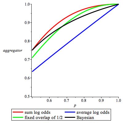
The left graph in Figure 4 provides a visual comparison of the above synthesis functions by graphing the diagonal values, that is those where . By symmetry, it suffices to graph each of these on the interval . When , both the average and the inverse-phi average are also equal to ; these are shown by the blue line. The red curve is , which is always greatest of the aggregators under consideration. The green and black curves represent and respectively, which are the two partial overlap models. As is evident, these are not strictly ordered. On the right, graphs are shown for and . When , as in the figure on the right, the inverse-phi average (shown in brown) is distinct from the average.
One final remark concerns , a popular choice for empirically driven aggregators. While it may seem atheoretical, in fact it arises as the limit as of the fixed overlap aggregator. To see this, denote the values of as varies over the algebra of sets generated by and by , , and ; thus and , where are independent Gaussians with respective variances .
As in Figure 5, asymptotically, the likeliest way to achieve and is to let and . These choices become forced in the limit. Applying this with and shows that the revealed forecast is which is the inverse-phi average. In other words, this forecast is practical only if we have reason to believe that both forecasters know nearly all information possible and that they find highly relevant information in the small part of their information that is not shared.
Acknowledgments
This research was supported in part by NSF grant # DMS-1209117
and a research contract to the University of Pennsylvania and the
University of California from the
Intelligence Advanced Research Projects Activity (IARPA)
via the Department of Interior National Business Center
contract number D11PC20061. The U.S. Government is authorized
to reproduce and distribute reprints for Government purposes
notwithstanding any copyright annotation thereon.
Disclaimer: The views and conclusions expressed herein are
those of the authors and should not be interpreted as necessarily
representing the official policies or endorsements, either expressed
or implied, of IARPA, DoI/NBC, or the U.S. Government.
REFERENCES
- [Dawid (1982)] Dawid, A. The well-calibrated Bayesian., Journal of the American Statistical Association. 77 (1982), 605–610.
- [Hong and Page (2009)] Hong, L. and Page, S. Interpreted and generated signals., Journal of Economic Theory. 144 (2009), 2174–2196.
- [Hwang and Pemantle (1997)] Hwang, J.T. and Pemantle, R. Estimating the truth of an indicator function of a statistical hypothesis under a class of proper loss functions., Statistics & Decisions. 15 (1997), 103–128.
- [Meyer (2009)] Meyer, C. The bivariate normal copula. Communications in Statistics–Theory and Methods. 42 (2009), 2402–2422.
- [Murphy and Winkler (1987)] Murphy, A. and Winkler, R. A general framework for forecast verification., Monthly Weather Review. 115 (1987), 1330–1338.
- [Parunak et al. (2013)] Parunak, H., Brueckner, S., Hong, L., Page, S. and Rohwer, R. Characterizing and aggregating agent estimates, In Proceedings of the 2013 International Conference on Autonomous Agents and Multi-agent Systems, pages 1021–1028. International Foundation for Autonomous Agents and Multi-agent Systems, Richland, SC. (2013).
- [Plackett (1954)] Plackett, R. A reduction formula for normal multivariate integrals., Biometrika. 41 (1954), 351–360.
- [Ravishanker and Dey (2001)] Ravishanker, N. and Dey, D. A First Course in Linear Model Theory. CRC Press (2001).
- [Satopää et al. (2014)] Satopää, V. and Pemantle, R. and Ungar, L. Modeling probability forecasts via information diversity,, To appear in Journal of the American Statistical Association. (2015).
- [Satopää et al. (2015)] Satopää, V., Jensen, S., Pemantle, R., and Ungar, L. Partial information framework: aggregating estimates from diverse information sources., Preprint. (2015).
- [Ungar et al. (2012)] Ungar, L., Mellers,B., Satopää, V., Tetlock, P. and Baron, J. The Good Judgment Project: A Large Scale Test of Different Methods of Combining Expert Predictions, In The Association for the Advancement of Artificial Intelligence 2012 Fall Symposium Series. (2012).