Quantum centipedes with strong global constraint

Consider a centipede with $N$ legs, moving along an infinite one-dimensional oriented regular lattice with unit spacing, and vertices labelled by integers, such that:
- each leg is attached to a vertex of the lattice, and at most one leg is attached to any given site (attachment constraint),
- any two consecutive legs are separated by at most one empty vertex, or gap (local constraint).
For a fixed position of the first (i.e. leftmost) leg, a configuration can be depicted by a sequence of regularly-spaced black and white bullets, with each black bullet corresponding to a leg attached to a vertex, and each white bullet corresponding to an empty vertex. Because of the attachment constraint, an allowed configuration contains exactly $N$ black bullets. For example, in the case $N=3$, the configuration of the legs allowed by the attachment constraint and the local constraint are the following:

$$(\bullet\bullet\bullet),\;(\bullet\circ\bullet\bullet),\;(\bullet\bullet\circ\bullet),\;(\bullet\circ\bullet\circ\bullet),$$

(1)

where the leftmost black dot on the left of each configuration is the first leg of the centipede (there are infinitely many empty vertices on the left of every configuration, as the lattice is infinite in both directions).

We can add a global constraint by requiring that the two external legs are at a distance at most $S$ from each other. The total length of the centipede is therefore between $N-1$ and $S$. The bound $S$ cannot be lower than $N-1$ because of the attachment constraint. If $S=N-1$, there is only one configuration allowed once the position of the first leg is chosen. Hence the value $S=N$ is the strongest global constraint on the length of the centipede still allowing the centipede to move.
In this note we focus on this case ($S=N$). Let us describe leg configurations. The only parameter in the model is $N$. If $N=2$, the local and global constraint are equivalent, and we are left with the two-body problem studied in [6]. Let us therefore assume that $N\geq 3$. There are $N$ allowed leg configurations for the centipede (if the position of the first leg is fixed):
- one in which there is no empty vertex between any pair of legs (the total length of the centipede is $N-1$ in this configuration), let us call it $l_{0}$;
- configurations in which exactly one pair of consecutive legs, say the $k$-th and $(k+1)$-th legs, are separated by one empty vertex; let us call such a configuration $l_{k}$, where $k$ can take all integer values between $1$ and $N-1$.
In the special case $N=3$, the first three configurations depicted in Eq. 1 are still allowed by the global constraint (they correspond to $l_{0}$, $l_{1}$ and $l_{2}$ respectively), while the last one is forbidden.

The allowed moves in an infinitesimal time step are of the following kinds.

$(i)$ From the configuration $l_{0}$ to either configuration $l_{1}$ or configuration $l_{N-1}$ (in the case $N=3$, these moves map $(\bullet\bullet\bullet)$ to $(\bullet\circ\bullet\bullet)$ and $(\bullet\bullet\circ\bullet)$ respectively), raising the length of the centipede to $N$, the largest value allowed by the global constraint.

$(ii)$ From the configuration $l_{k}$ (with $k$ an integer in $[1..N-2]$ to either the configuration $l_{k-1}$ or the configuration labelled $l_{k+1}$ (in the case $N=3$, these moves map $(\bullet\circ\bullet\bullet)$ to $(\bullet\bullet\bullet)$ and $(\bullet\bullet\circ\bullet)$ respectively, either conserving the length of the centipede, or reducing ot by one).

$(iii)$ From the configuration $l_{N-1}$ to either the configuration $l_{N-2}$ or to the configuration $l_{0}$ (in the case $N=3$, these moves map $(\bullet\bullet\circ\bullet)$ to $(\bullet\circ\bullet\bullet)$ and $(\bullet\bullet\bullet)$ respectively, conserving the length of the centipede in the first case, reducing the length by one in the second case, but without moving the first leg, unlike the move described in $(ii)$ that maps the configuration to $l_{0}$).

Let us describe the quantum walk of the centipede by the wave function $|\psi(t)\rangle$, which lives in the Hilbert space $\mathcal{H}_{N}$ consisting of the tensor product of the position of the first leg and the space spanned by the above-described configurations of legs:

$$|\psi(t)\rangle\in\mathcal{H}_{N}=\mathbf{Z}\otimes{\mathrm{Span}}_{\mathbf{C}}(\left\{|l_{k}\rangle\right\}_{0\leq k\leq N-1}).$$

(2)

where $|l_{k}\rangle$ is the ket corresponding to the leg configuration denoted by $l_{k}$.

If the position of the first leg is fixed at the vertex labelled $n$ (corresponding to the ket $|n\rangle$), the wave function of the centipede at time $t$ can therefore be described as an element of the projection of the Hilbert space $\mathcal{H}_{N}$ onto the ket $|n\rangle$:

$$|\psi_{n}(t)\rangle=\langle n|\psi(t)\rangle.$$

(3)

Let us introduce the Fourier transform of the wave function, by defining for every wave number $q$ in the first Brillouin zone

$$|\hat{\psi}(q,t)\rangle=\sum_{n\in\mathbf{Z}}e^{-inq}|\psi_{n}(t)\rangle.$$

(4)

The ket $|\hat{\psi}(q,t)\rangle$ is an element of the $N$-dimensional span of the leg configurations:

$$|\hat{\psi}(q,t)\rangle\in{\mathrm{Span}}_{\mathbf{C}}(\left\{|l_{k}\rangle\right\}_{0\leq k\leq N-1}).$$

(5)

For a fixed wave number $q$, the allowed moves in continuous time (with identical rates) that have been described in $(i)$–$(iii)$ induce a Schrödinger equation for the Fourier transform $|\hat{\psi}(q,.)\rangle$, with a $q$-dependent Hamiltonian:

$$i\frac{\partial}{\partial t}|\hat{\psi}(q,t)\rangle=H(q)|\hat{\psi}(q,t)\rangle,$$

(6)

where the Hamiltonian operator $H(q)$ is expressed as

$$H(q)=J(q)+J(q)^{\dagger},$$

(7)

with the entry of the $N$ by $N$ matrix of $J(q)$ at row $i$ and column $j$ (in the basis $\left\{|l_{k}\rangle\right\}_{0\leq k\leq N-1}$) is given by

$$(J(q))_{ij}=e^{-iq}\delta_{i1}\delta_{j2}+\delta_{iN}\delta_{j1}+\sum_{j=3}^{N}\delta_{i,j-1}.$$

(8)

In the case $N=3$, we obtain¹¹ 1 As $N$ is the only parameter in the model, we exclude the symbol $N$ from most notations, making the dependence on $N$ implicit, but restore it for definiteness when describing the case $N=3$. the following matrices:

$$J(q)_{(N=3)}=\left(\begin{array}[]{lll}0&e^{-iq}&0\\ 0&0&1\\ 1&0&0\end{array}\right),\;\;\;H(q)_{(N=3)}=\left(\begin{array}[]{lll}0&e^{-iq}&1\\ e^{iq}&0&1\\ 1&1&0\end{array}\right).$$

(9)

The $q$-dependent matrix elements in the Hamiltonian reflect the fact that the only allowed moves that modify the position of the first leg of the centipede are the moves from configuration $l_{0}$ to configuration $l_{1}$, and from $l_{1}$ to configuration $l_{0}$ (together with the definition of the Fourier transform, Eq. 4). The rules assigning the values $e^{iq}$, $e^{-iq}$ or $1$ to matrix elements of the Hamiltonian according to configuration moves are identical to the ones worked out in [7] (see Eqs. (3.7) in Section 3 of that paper). The effect of the global constraint is just to reduce the set of allowed configurations and moves, ensuring that the Hamiltonian $H(q)$ is a submatrix extracted from the matrix of size $2^{N-1}$ corresponding to the dynamics of a centipede with the same number of quantum walkers, identical local constraints and no global constraint.

The Hamiltonian $H(q)$ can be diagonalised using the same method as for a circulant matrix (to which it reduces if $e^{iq}$ equals 1). Indeed, we can diagonalise $J(q)$ and $J(q)^{\dagger}$ separately, and notice that they have the same eigenvectors (associated to complex conjugated eigenvalues). These eigenvectors are therefore those of the Hamiltonian, and they are associated to eigenvalues equal to twice the real part of those of $J(q)$.

Let us denote by $|u\rangle=\sum_{j=0}^{N-1}u_{j}|l_{j}\rangle$ an eigenvector of $J(q)$, and by $\lambda$ the associated eigenvalue. The components satisfy the system of equations:

$$e^{-iq}u_{1}=\lambda u_{0},$$

$$\forall j\in[1..(N-2)],\;u_{j+1}=\lambda u_{j},$$

$$u_{0}=\lambda u_{N-1}.$$

This system implies

$$\forall j\in[1..(N-1)],\;u_{j}=\lambda^{j-1}e^{iq}u_{0},$$

$$u_{0}=\lambda^{N}e^{iq}u_{0}.$$

The component $u_{1}$ cannot be zero, otherwise the eigenvector $|u\rangle$ would be zero, hence the eigenvalue $\lambda$ must satisfy

$$\lambda^{N}e^{iq}=1.$$

(10)

The eigenvalues of $J(q)$ are therefore elements of the set of complex numbers

$$\left\{\lambda_{k}(q)=e^{\frac{i}{N}\left(-q+2k\pi\right)},\;k\in[0..N-1]\right\}.$$

(11)

Moreover, using the system of equations, one can check that for fixed $k$ in $[0..N-1]$ the ket

$$|u^{(k)}(q)\rangle=\frac{1}{\sqrt{N}}\sum_{j=0}^{N-1}\lambda_{k}(q)^{j}e^{-iq\delta_{j0}}|l_{j}\rangle$$

(12)

is a normalized eigenvector of $J(q)$ associated with the eigenvalue $\lambda_{k}(q)$. Moreover, it is an eigenvector of $J(q)^{\dagger}$ associated with the eigenvalue $\lambda_{k}^{-1}$. It is therefore an eigenvector of the Hamiltonian $H(q)$ associated with the eigenvalue $\lambda_{k}+\lambda_{k}^{-1}$. The spectrum of $H(q)$ therefore consists of $N$ eigenvalues expressed as cosines with regularly spaced arguments:

$${\mathrm{Spec}}\left(H(q)\right)=\left\{\omega_{k}(q)=2\cos\left(\frac{1}{N}\left(-q+2k\pi\right)\right),\;k\in[0..N-1]\right\}$$

(13)

The group velocities corresponding to these modes read

$$v_{k}(q)=\frac{\partial}{\partial q}\omega_{k}(q)=\frac{2}{N}\sin\left(\frac{1}{N}\left(-q+2k\pi\right)\right),\;k\in[0..N-1].$$

(14)

The maximal absolute value $V^{(N)}$ of the group velocities of the strongly constrained $N$-legged quantum centipede

$$V^{(N)}=\mathrm{max}_{q\in[-\pi,\pi],k\in[0..N-1]}|v_{k}(q)|$$

(15)

therefore goes to zero in the large-$N$ limit. If $N$ is a multiple of 4, the sine function reaches its maximal value at $q=0$, along the branch corresponding to $k=N/4$. If $N$ is large enough, considering the division of $N$ by 4 is enough to see that the maximal possible value of the group velocities is always reached.

Consider the initial condition corresponding to a centipede with the first leg at the origin and no empty vertex between any pair of legs:

$$|\psi_{n}(0)\rangle=\delta_{n,0}|l_{0}\rangle,\;\forall n\in{\mathbf{Z}}.$$

(16)

Rewriting the position of the leftmost leg as an integral over Fourier modes, and using the basis $\left\{|l_{k}\rangle\right\}_{0\leq k\leq N-1}$ of the space of leg configurations, we can integrate the Schrödinger equation (Eq. 6) as follows:

$$|\psi_{n}(0)\rangle=\int_{0}^{2\pi}\frac{dq}{2\pi}e^{inq}\sum_{k=0}^{N-1}\langle u^{(k)}|l_{0}\rangle|u^{(k)}(q)\rangle,$$

(17)

$$|\psi_{n}(t)\rangle=\int_{0}^{2\pi}\frac{dq}{2\pi}e^{inq}\sum_{k=0}^{N-1}\langle u^{(k)}(q)|l_{0}\rangle e^{-i\omega_{k}t}|u^{(k)}(q)\rangle.$$

(18)

Substituting the results of the diagonalisation of $H(q)$, Eqs 11 and 12, we express the ket $|\psi_{n}(t)\rangle$ as a sum over eigenvectors:

$$|\psi_{n}(t)\rangle=\frac{1}{\sqrt{N}}\int_{0}^{2\pi}\frac{dq}{2\pi}e^{i(n+1)q}\sum_{k=0}^{N-1}e^{-2it\cos\left(\frac{-q+2k\pi}{N}\right)}|u^{(k)}(q)\rangle.$$

(19)

The probability law of the position of the first leg at time $t$ is obtained by adding together the probabilities of the configurations with the same position of the first leg:

$$P_{n}(t)=\sum_{p=0}^{N-1}|\langle l_{p}|\psi_{n}(t)\rangle|^{2}=\frac{1}{N}\sum_{p=0}^{N-1}\left|\int_{0}^{2\pi}\frac{dq}{2\pi}\sum_{k=0}^{N-1}e^{i(n+1)q-2it\cos\left(\frac{-q+2k\pi}{N}\right)}\langle l_{p}|u^{(k)}(q)\rangle\right|^{2}.$$

(20)

Using Eq. 12 for the components of the eigenvectors of $H(q)$ yields integrands in exponential form:

$$P_{n}(t)=\frac{1}{N^{2}}\sum_{p=0}^{N-1}\left|\int_{0}^{2\pi}\sum_{k=0}^{N-1}\frac{dq}{2\pi}e^{i(n+1)q-2it\cos\left(\frac{-q+2k\pi}{N}\right)}\lambda_{k}(q)^{p}(e^{-iq}\delta_{0p}+(1-\delta_{0p}))\right|^{2}.$$

(21)

In the integral corresponding to index $k$, let us perform the change of variable

$$K=\frac{-q+2k\pi}{N},$$

(22)

which results in $k$-dependent bounds in the integrals (with no dependence on the integer $k$ left in the integrand, due to periodicity):

$$P_{n}(t)=\sum_{p=0}^{N-1}\left|\sum_{k=0}^{N-1}\int_{\frac{2k\pi}{N}}^{\frac{2(k+1)\pi}{N}}\frac{dK}{2\pi}e^{i(-(n+1)N+p)K-2t\cos K)}(e^{iNK}\delta_{0p}+(1-\delta_{0p}))\right|^{2}.$$

(23)

The sum over the integer $k$ can therefore be performed by extending the integration domain to the full interval $[0,2\pi]$, yielding Bessel functions according to the integral definition:

$$J_{m}(t)=i^{m}\int_{0}^{2\pi}\frac{dq}{2\pi}e^{i(mq-t\cos q)},$$

(24)

so that each value of the index $p$ in Eq. 23 yields a Bessel function:

$$P_{n}(t)=\left(|J_{(-nN)}(2t)|^{2}+\sum_{p=1}^{N-1}|J_{p-(n+1)N}(2t)|^{2}\right).$$

(25)

This closed-form expression is reminiscent of the case of a single quantum walker, in which only one Bessel function appears in the wave function [6].

Consider a centipede with $N$ legs, and allow a weaker global constraint on the maximal total distance between the first and last legs, $S\geq N$. Let us keep the local constraint on the maximal number of empty sites between two consecutive legs. The maximal total number $G$ of gaps allowed between legs is $G=S-N+1$. The case $G=1$ has been solved exactly, let us now assume $G>1$. A basis of the Hilbert space is given by the direct sum of spaces of linear combinations of configurations with a fixed number $g$ of gaps, for $g$ in $[0..G]$. The value $g=0$ corresponds to just one configuration, with length $N-1$. At a fixed value $g>1$, the allowed configurations are in one-to-one correspondence with the number of ways of choosing $g$ distinct integers $p_{1},\dots,p_{g}$, with $1\leq p_{1}<\dots<p_{g}<N$, where $p_{k}$ is the index of the $k$-th leg that is followed by a gap. If $g>1$, we can rewrite the last index $p_{g}$ by grouping consecutive indices as follows:

$$p_{g}=p_{1}+\sum_{k=2}^{g}(p_{k}-p_{k-1}),$$

(26)

which induces a $(g+1)$-composition²² 2 A composition of an integer $n$ with $k$ terms (or $k$-composition) is a way to write $n$ as a sum of $k$ strictly positive integers, i.e. an element $(u_{1},\dots,u_{k})$ of $({\mathbf{N}}^{\ast})^{k}$, such that $n=\sum_{p=1}^{k}u_{p}$. The order of the terms is taken into account: two $k$-compositions $(u_{1},\dots,u_{k})$ and $(u^{\prime}_{1},\dots,u^{\prime}_{k})$ of $n$ are regarded as identical if and only if $\sum_{p=1}^{k}|u_{p}-u^{\prime}_{p}|=0$. If $n>1$ and $k>1$, the $k$-compositions of $n$ are in one-to-one correspondence with a choice of $k-1$ spacings between consecutive integers in $[1..n]$ (in our case, the role of $k-1$ is played by the number of gaps). As there are $n-1$ such spacings, there are ${{n-1}\choose{k-1}}$ distinct $k$-compositions of $n$. This expression also yields the correct result if $k=1$. of $N$:

$$N=p_{g}+N-p_{g}=p_{1}+\sum_{k=2}^{g}(p_{k}-p_{k-1})+(N-p_{g}),$$

(27)

corresponding to a description of the configuration in terms of the cardinalities of sets of consecutive legs that do not contain any gap, read from left to right.

Conversely, given a $(g+1)$-composition $(s_{1},\dots,s_{g+1})$ of $N$, it can be mapped to an allowed configuration with $g$ gaps, by concatenating $(g+1)$ sets of legs with $s_{k}$ legs each, spaced by one gap. The allowed configurations at fixed length $N-1+g$ are therefore in one-to-one correspondence with the $(g+1)$-compositions of $N$. Let us denote by $\mathcal{C}_{g,N}$ the corresponding subspace of the Hilbert space. The Fourier modes of the wave function of the constrained quantum centipede are therefore elements of the direct sum of these spaces, for all values of $g$ compatible with the global constraint:

$$|\hat{\psi}(q,t)\rangle\in\bigoplus_{g=0}^{S-N+1}\mathcal{C}_{g,N},$$

(28)

and from the above discusion

$${\mathrm{dim}}\;\mathcal{C}_{g,N}={{N-1}\choose{g}}.$$

(29)

The Hamiltonian $H(q)$ can be expressed in matrix form, with a block structure adapted to the decomposition of the Hilbert space in Eq. 29. This requires a choice of order in each of the relevant sets of compositions, but the spectrum of the Hamiltonian does not depend on this choice. For numerical implementation we can choose the lexicographic order. The general rules allowing the centipede to move one leg at a time induce couplings within a given diagonal block corresponding to compositions with a fixed number of terms differing by the transfer of one unit between two adjacent terms. The corresponding entries in the matrix of the Hamiltonian equal one. All the non-zero elements in non-diagonal blocks couple configurations belonging to blocks $\mathcal{C}_{g,N}$ and $\mathcal{C}_{g^{\prime},N}$, with $|g-g^{\prime}|=1$. Such couplings involve pairs of compositions, one of which has a $1$ in initial (resp. final) position (in which case the corresponding entry in the Hamiltonian equals $e^{\pm iq}$, resp. $1$) or terminal position. A heat map of the real part of the Hamiltonian with these conventions for $N=16$ and $S=17$ (corresponding to a maximal of $G=2$ two gaps in configurations) is illustrated in Fig. 1.

In the notations introduced above in the case of the strongest constraint $S=N$, the integer $j$ labelling the configurations yields a basis of the one-dimensional space $\mathcal{C}_{0,M}$ for $j=0$, while each of the remaining $N-1$ values of $j$ corresponds to the two-composition $N=j+(N-j)$. As the configuration with no gaps was put in the first position in the basis of the Hilbert space in Section 2, the presentation of the Hamiltonian in matrix form so far is consistent with the block structure adapted to compositions of $N$.

Given the number $N$ of legs of the centipedes, and the total number $G$ of gaps between legs allowed by the global constraint, assuming a choice of order in the elements of the basis, let us denote by $H(q)$ the matrix form of the Hamiltonian. The $q$-dependent entries are equal either to $e^{iq}$ or to $e^{-iq}$. Let us denotes by $B$ the sub-matrix of $H(q)$ containing only entries equal to 0 or 1 for all values of the mode $q$. There is a matrix unique $A$ with entries equal to 0 or 1, such that the following relation holds for all $q$ in $[-\pi,\pi]$:

$$H(q)=e^{iq}A+e^{-iq}A^{\dagger}+B.$$

(30)

Given the spectrum of phase velocities and associated eigenvectors of $H(q)$, labelled by the integer $k$ and a functional dependence on the mode $q$, the group velocities at mode $q^{\prime}=q+\epsilon$ close to $q$ can be computed using first-order perturbation theory (assuming non-degeneracy):

$$H(q)|\psi_{(k)}(q)\rangle=\omega_{k}(q)|\psi_{(k)}(q)\rangle,\;\;\forall q\in[-\pi,\pi],$$

(31)

$$H(q+\epsilon)=H(q)+\epsilon(ie^{iq}A-e^{-iq}A^{\dagger})+o(\epsilon),$$

(32)

so that the group velocities at mode $q$ are expressed as

$$\frac{\partial\omega_{k}}{\partial q}(q)=\langle\psi_{(k)}(q)|(ie^{iq}A-ie^{-iq}A^{\dagger})|\psi_{(k)}(q)\rangle.$$

(33)

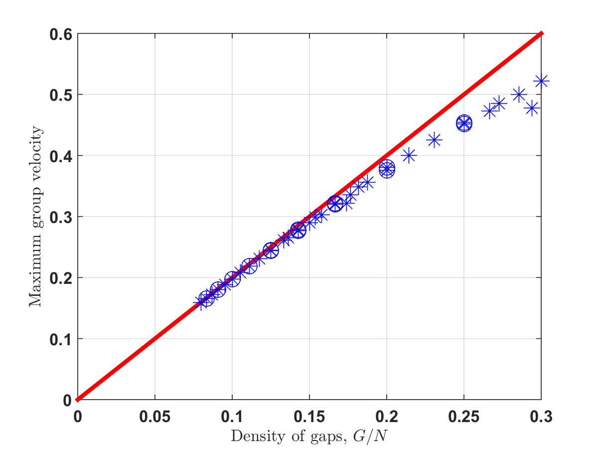
The implementation³³ 3 in MATLAB, code available online at Researchgate, https://www.researchgate.net/publication/315625145, with regularly spaced modes in the interval $[-\pi,\pi]$, yields the spectra plotted in Fig. 2 for $N=5$. It allows to reproduce the relevant figures of [7] in the case $G=N-1$, corresponding to a fully relaxed global constraint. When the maximal group velocity is plotted at fixed value of $N$ as a function of $G$, the rate of growth can be observed between the value $2/N$ and the saturation value predicted in [7]. The plot of Fig. 3 exhibits a linear growth at small values of $G$. The propagation of wave packets yield heuristic arguments explaining this behaviour.

Consider a quantum centipede with a large number $N$ of legs and a global constraint corresponding to a maximal number $G$ of gaps. Let us assume that $G$ is a divisor of $N$, so that there exists configurations with $G$ gaps obtained by concatenating $G$ identical configurations of a centipede with $L=N/G$ legs and one gap. There must also be wave packets with maxima spaced by $L$. If $L$ is large enough, the maxima of these wave packets should be well separated, and as the number of maxima equals the maximal number of gaps, the propagation of such wave packets should be well approximated at short times by the concatenation of $G$ wave packets, each of which is propagating on a maximally constrained centipede with $L$ legs.

Consider such a wave packet, described by a wave function $\phi$ in Fourier space, assumed to be peaked at the value $q_{0}$ of the linear momentum, and containing only modes from the branch of index $k$ of the spectrum of the maximally constrained Hamiltonian, such that $\partial_{q}\omega_{k}(q_{0})$ is the maximal group velocity. The corresponding wave function in position space, denoted by $\tilde{\phi}$, can be expressed in terms of its projections on the kets $|l_{p}\rangle$, for $p$ between $0$ and $L-1$:

$$\begin{split}\langle l_{p}|\tilde{\phi}_{n}\rangle(t)&=\int_{0}^{2\pi}dq\,\phi(q)e^{i(qn-\omega_{k}(q)t)}\langle l_{p}|u_{k}(q)\rangle\\ &=\frac{1}{\sqrt{L}}\int_{0}^{2\pi}dq\,\phi(q)\exp\left(i\left(q(n+\delta_{j0}-\omega_{k}(q)t+\frac{p}{L}(q+2k\pi)\right)\right).\end{split}$$

(34)

With the dispersion relation of Eq. 13, the derivatives of all even orders of $\omega_{k}(q)$ vanish at the extremum $q_{0}$, while the derivatives of odd order $(2j+1)$ are proportional to the maximal group velocity:

$$\frac{\partial^{2j+1}\omega}{\partial x^{2j+1}}(q_{0})=\frac{2}{L^{2j+1}}.$$

(35)

The time-evolution of a wave packet traveling at the maximal group velocity is therefore given by

$$\begin{split}\langle l_{p}|\tilde{\phi}_{n}\rangle&=\int_{0}^{2\pi}dq\,\phi(q)e^{i(qn-\omega_{k}(q)t)}\langle l_{p}|u_{k}(q)\rangle\\ &=\frac{1}{\sqrt{L}}\int_{0}^{2\pi}dq\,\phi(q)\exp\left(i\left(q(n+\delta_{p0})-2\sinh\left(\frac{q-q_{0}}{L}\right)t+\frac{p}{L}(q+2k\pi)\right)\right).\end{split}$$

(36)

If the density of modes $\phi$ is sufficiently peaked around $q_{0}$, the wave front travels at velocity $2/L$. As the space is discrete, the characteristic time step for this evolution to be detectable is $\delta t=L/2$. For the concatenation of $G$ such short wave packets to yield a wave packet with fronts traveling at velocity $2/L$, the deformation of the wave packet $\tilde{\phi}$ must be small over the time interval $\delta t$. A large-$L$ expansion at first non-trivial order yields

$$\langle l_{p}|\tilde{\phi}_{n}\rangle(\delta t)=\left(e^{2i\frac{q_{0}}{\delta t}}\langle l_{p}|\tilde{\phi}_{n-\frac{2\delta t}{L}}\rangle(0)\right)\left(1+O(L^{-3}\delta t\right)),$$

(37)

which shows that the description of the propagation as a traveling wave packet, over a time step $\delta t=L/2$, should become better for larger $N$ at fixed $G$.

In real space, starting from a concatenation of $G$ such short wavepackets spread over a segment of length $L$ each. At fixed $L$, that is at a fixed value of the group velocity of each wave packet, the fraction of the probability measure of the centipede that will feel boundary effects over an interval of $L$ units of time corresponds to the two short wave packets that are close to the first and last leg of the centipede. It is is proportional to $G^{-1}=L/N$, which goes to zero with $N$. At a fixed value of the intensive variable $G/N$ (the maximal density of gaps along the centipede), the proposed concatenation of short wave packets should become a better approximation to a long wave packet traveling at group velocity $2G/N$ when $N$ grows.

Plotting the maximal group velocities as a function of the maximal allowed density of gaps $G/N$ reveals a linear growth, with negative corrections due to the saturation phenomenon (see Fig. 4). The fact that the linearity has been tested numerically within 4 percent of the predicted value at $L=6$ for low values of $N$ suggests lower bounds on the group velocities that can be reached at large $N$ for a fixed value of the denisty of gaps. For instance a finite group velocity of about $0.26$ should be reachable in the large-$N$ limit with a maximal allowed density of gaps of about 16 percent, or $G=0.16N$. Values of $G$ that are not divisors of $N$ roughly yield a growing maximal group velocity as a function of the density, even though the above argument is not valid for them, as the group velocities of the short wave packets cannot be uniform across the concatenation. This effect should become less relevant when $N$ goes to infinity.

On the other hand, at a fixed value of $N$, the maximal group velocity is expected to be a growing function of the total number $G$ of gaps allowed, and to be smaller than the value $V^{(N)}$ obtained if no global constraint is imposed. This value decreases exponentially fast as a function of $N$, to reach a limit $V^{(\infty)}$ expressed in integral form in [7] and evaluated numerically to be $V^{\infty}\simeq 0.570$. The linear growth of the maximal group velocity in the globally constrained model as a function of the density of gaps $G/N$ can therefore not keep going after this value of the group velocity is reached. This yields an upper bound $G_{crit}$ on the number of gaps for which the maximal group velocity can be estimated by linear extrapolation of the model with strongest global constraint:

$$\frac{2(G_{crit})}{N}=V^{\infty},\;\;\;{\mathrm{i.e.}}\;\;\;G_{crit}\simeq[0.2852N].$$

(38)

This upper bound grows as $O(N)$ and thanks to the fast convergence to $V^{\infty}$ yields numerically testable cases (some of which are visible on Fig. 3).

References

- [1] E. R. Kay, D. A. Leigh, and F. Zerbetto, Angew. Chem. Int. Ed. 46, 72–191 (2007).
- [2] T. Antal, P.L. Krapivsky and K. Mallick, Molecular spiders in one dimension, J. Stat. Mech. (2007) P08027, [arXiv:0705.2594].
- [3] Y. Aharonov, L. Davidovich L and N. Zagury, Quantum random walks, Phys. Rev. A 48 1687.
- [4] J. Kempe, Quantum random walks – an introductory overview, Contemp. Phys. 44 307.
- [5] S. de Toto Arias and J.M. Luck, Anomalous dynamical scaling and bifractality in the 1D Anderson model de Toto Arias, Journal of Physics A 31 (1998), 7699, [arXiv:cond-mat/9808021].
- [6] P.L. Krapivsky, J.M. Luck and K. Mallick, Interacting quantum walkers: Two-body bosonic and fermionic bound states, J. Phys. A: Math. Theor. 48 475301, [arXiv:1507.01363].
- [7] P.L. Krapivsky, J.M. Luck and K. Mallick Quantum centipedes: collective dynamics of interacting quantum walkers, J. Phys. A 49, 335303 (2016), [arXiv:1603.04601].