跳到论文正文
W Papers独立论文阅读器 arXiv:1608.04223 论文正文 计算阅读时间 · 0%
引用这篇论文根据当前论文元数据生成,正式投稿前建议核对。


License: arXiv.org perpetual non-exclusive license
arXiv:1608.04223v4 [cs.DS] 27 Dec 2017

A Faster Approximation Algorithm for the Gibbs Partition Function

Vladimir Kolmogorov Affiliation: Institute of Science and Technology Austria Email: vnk@ist.ac.at
Abstract

We consider the problem of estimating the partition function Z⁡(β)=∑xexp⁡(−β​H​(x))Z(\beta)=\sum_{x}\exp(-\beta H(x)) of a Gibbs distribution with a Hamilton H⁡(⋅)H(\cdot), or more precisely the logarithm of the ratio q=ln⁡Z⁡(0)/Z⁡(β)q=\ln Z(0)/Z(\beta). It has been recently shown how to approximate qq with high probability assuming the existence of an oracle that produces samples from the Gibbs distribution for a given parameter value in [0,β][0,\beta]. The current best known approach due to Huber [9] uses O⁡(q​ln⁡n⋅[ln⁡q+ln⁡ln⁡n+ε−2])O(q\ln n\cdot[\ln q+\ln\ln n+\varepsilon^{-2}]) oracle calls on average where ε\varepsilon is the desired accuracy of approximation and H⁡(⋅)H(\cdot) is assumed to lie in {0}∪[1,n]\{0\}\cup[1,n]. We improve the complexity to O⁡(q​ln⁡n⋅ε−2)O(q\ln n\cdot\varepsilon^{-2}) oracle calls. We also show that the same complexity can be achieved if exact oracles are replaced with approximate sampling oracles that are within O⁡(ε2q​ln⁡n)O(\frac{\varepsilon^{2}}{q\ln n}) variation distance from exact oracles. Finally, we prove a lower bound of Ω⁡(q⋅ε−2)\Omega(q\cdot\varepsilon^{-2}) oracle calls under a natural model of computation.

1 Introduction

It is known that for large classes of problems, e.g. self-reducible problems [14], there is an intimate connection between approximate counting and sampling: the ability to solve one problem allows solving the other one. This paper explores this connection for Gibbs distributions.

Let Ω\Omega be some finite set and H⁡(⋅)H(\cdot) be some real-valued function on Ω\Omega called a Hamiltonian. The Gibbs distribution for such a system is a family of distributions {μβ}\{\mu_{\beta}\} on Ω\Omega parameterized by β\beta, where

μβ​(x)=1Z⁡(β)​exp⁡(−β​H​(x))∀x∈Ω\mu_{\beta}(x)=\frac{1}{Z(\beta)}\exp(-\beta H(x))\hskip 20.00003pt\forall x\in\Omega (1)

The normalizing constant Z⁡(β)Z(\beta) is called the partition function:

Z⁡(β)=∑x∈Ωexp⁡(−β​H​(x))Z(\beta)=\sum_{x\in\Omega}\exp(-\beta H(x)) (2)

Estimating this function for a given value of β\beta is a widely studied computational problem with applications in many areas. In particular, it is a key computational task in statistical physics. Evaluations of Z⁡(⋅)Z(\cdot) yield estimates of important thermodynamical quantities, such as the free energy. Note, parameter β\beta corresponds to the inverse temperature. A classical example of a Gibbs distribution in physics is the Ising model.

Example 1.

Given an undirected graph (V,E)(V,E), let Ω={−1,+1}V\Omega=\{-1,+1\}^{V} and H(x)=∑{i,j}∈E[xi≠xj]H(x)=\sum_{\{i,j\}\in E}[x_{i}\neq x_{j}] where [⋅][\cdot] is 1 if its argument is true, and 0 otherwise. Distribution (1) for such a Hamiltonian is called the Ising model. It is ferromagnetic if β>0\beta>0, and antiferromagnetic if β<0\beta<0 (although in the latter case the function H′​(x)=−H​(x)H^{\prime}(x)=-H(x) is usually treated as the Hamiltonian). Computing Z⁡(β)Z(\beta) exactly is a #\#P-complete problem, and is even hard to approximate in the antiferromagnetic case [13].

The problem of counting various combinatorial objects such as proper kk-coloring and matchings in graphs can also be naturally phrased as estimating the partition function.

Example 2.

Let Ω={1,…,k}|V|\Omega=\{1,\ldots,k\}^{|V|} be the set of all colorings in an undirected graph G=(V,E)G=(V,E). Define H(x)=∑{i,j}∈E[xi=xj]H(x)=\sum_{\{i,j\}\in E}[x_{i}=x_{j}], then Z⁡(+∞)Z(+\infty) gives the number of proper kk-colorings.

Example 3.

Let Ω\Omega be the set of matchings M⊆EM\subseteq E in an undirected graph G=(V,E)G=(V,E). Define H⁡(M)=|M|H(M)=|M|, then Z⁡(0)=|Ω|Z(0)=|\Omega|.

A related problem is that of sampling from the distribution μβ\mu_{\beta} for a given value of β\beta. There is a vast literature on designing sampling algorithms from Gibbs distributions, see e.g. [17, 19, 8, 6] or [4] for an overview. For the ferromagnetic Ising model there exists a polynomial-time approximate sampling algorithm [13] and also an exact sampling algorithm that appears to run efficiently at or above the critical temperature [18]. Approximate sampling of kk-colorings in low-degree graphs is addressed in [12, 21] (for β=+∞\beta=+\infty, though techniques are potentially extendable to other values of β\beta), and for matchings polynomial-time approximate sampling is described in [16, Section 2.3.5].

It is known that the ability to sample can be used for designing a randomized approximation scheme for estimating the partition function. By definition, it is an algorithm that for a given ε>0\varepsilon>0 produces an estimate Q^\hat{Q} of the desired quantity QQ such that Q^∈[Q1+ε,Q⁡(1+ε)]\hat{Q}\in\left[\frac{Q}{1+\varepsilon},Q(1+\varepsilon)\right] with probability at least 3/43/4. (The value 3/43/4 is arbitrary: by repeating the algorithm multiple times and taking the median of the outputs the probability can be boosted to any other constant in (0,1)(0,1)). This paper studies the following question: how many samples are needed to approximate Z⁡(β)Z(\beta) with a given accuracy ε\varepsilon?

Formal description   To state the complexity of different approaches, we need to introduce several quantities. First, we assume that H⁡(x)∈{0}∪[1,n]H(x)\in\{0\}\cup[1,n] for any x∈Ωx\in\Omega where nn is a known number. Non-negativity of the Hamiltonian implies that Z⁡(⋅)Z(\cdot) is a decreasing function. Our goal will be to estimate the ratio Q=Z⁡(βmin)/Z⁡(βmax)Q=Z({\beta_{\min}})/Z({\beta_{\max}}) for given values βmin<βmax{\beta_{\min}}<{\beta_{\max}}. Note that computing Z⁡(β)Z(\beta) for some specific value of β\beta is usually an easy task, so this will allow estimating Z⁡(β)Z(\beta) for any other β\beta. In particular, in Examples 1, 2 and 3 we have Z⁡(0)=2|V|Z(0)=2^{|V|}, Z⁡(0)=k|V|Z(0)=k^{|V|} and Z⁡(+∞)=1Z(+\infty)=1 respectively.

Let us denote q=log⁡Qq=\log Q, and assume that there exists an oracle that can produce a sample X∼μβX\sim\mu_{\beta} for a given value β∈[βmin,βmax]\beta\in[{\beta_{\min}},{\beta_{\max}}]. When stating asymptotic complexities, we will always assume that q=Ω⁡(1)q=\Omega(1), n=1+Ω⁡(1)n=1+\Omega(1) and ε=O⁡(1)\varepsilon=O(1) to simplify the expressions. Bezáková et al. [2] showed that QQ can be estimated using O⁡(q2​(ln⁡n)2)O(q^{2}(\ln n)^{2}) oracle calls in the worst case (for a fixed ε\varepsilon). This was improved to O⁡(q​(ln⁡q+ln⁡n)5​ε−2)O(q(\ln q+\ln n)^{5}\varepsilon^{-2}) expected number of calls by Štefankovič et al. [22] and then to O⁡(q​ln⁡n⋅[ln⁡q+ln⁡ln⁡n+ε−2])O(q\ln n\cdot[\ln q+\ln\ln n+\varepsilon^{-2}]) by Huber [9].

The first contribution of this paper is to improve the complexity further to O⁡(q​ln⁡n⋅ε−2)O(q\ln n\cdot\varepsilon^{-2}) oracle calls (on average). This is achieved by a better analysis of the algorithm in [9]. The formal statement of our result is given in Section 3 as Theorems 5 and 7.

In many applications we only have an access to approximate sampling oracles. Using a standard coupling argument, in Section 3.1 we show that the same complexity can be achieved with approximate oracles assuming that they are within O⁡(ε2q​ln⁡n)O(\frac{\varepsilon^{2}}{q\ln n}) variation distance from exact oracles.

As our final contribution, we prove a lower bound of Ω⁡(q⋅ε−2)\Omega(q\cdot\varepsilon^{-2}) oracle calls under a natural model of computation. The precise statement of the result is given as Theorem 12 in Section 5.

Remark 1.

The assumption that H⁡(⋅)H(\cdot) lies in {0}∪[1,n]\{0\}\cup[1,n] can be relaxed using a standard trick. Suppose, for example, that H⁡(x)∈{hmin,hmin+1,…,hmax}H(x)\in\{h_{\min},h_{\min}+1,\ldots,h_{\max}\} where hminh_{\min} and hmaxh_{\max} are known integers. Let n=hmax−hminn=h_{\max}-h_{\min}. We claim that the problem can be solved using O⁡(q′​ln⁡n⋅ε−2)O(q^{\prime}\ln n\cdot\varepsilon^{-2}) oracle calls (on average), where either (i) q′=q−(βmax−βmin)⋅hminq^{\prime}=q-({\beta_{\max}}-{\beta_{\min}})\cdot h_{\min}, or (ii) q′=−q+(βmax−βmin)⋅hmaxq^{\prime}=-q+({\beta_{\max}}-{\beta_{\min}})\cdot h_{\max}.

Indeed, to achieve the first complexity, define new Hamiltonian H′​(x)=H⁡(x)−hminH^{\prime}(x)=H(x)-h_{\min}. The partition function for the new problem is Z′​(β)=eβ​hmin⋅Z⁡(β)Z^{\prime}(\beta)=e^{\beta h_{\min}}\cdot Z(\beta), and so q′q^{\prime} is as defined in (i). (We use “primes” to denote all quantities related to the new problem). We have H′​(x)∈{0,1,…,n}H^{\prime}(x)\in\{0,1,\ldots,n\}, so the algorithm claimed above can be applied to give an estimate of q′q^{\prime} and thus of qq. Note that distributions μβ′\mu^{\prime}_{\beta} and μβ\mu_{\beta} coincide, and so sampling from μβ\mu_{\beta} allows to sample from μβ′\mu^{\prime}_{\beta}.

To achieve the second complexity, define H′​(x)=−H⁡(x)+hmaxH^{\prime}(x)=-H(x)+h_{\max} and also change the bounds: βmin′=−βmax\beta^{\prime}_{\min}=-{\beta_{\max}} and βmax′=−βmin\beta^{\prime}_{\max}=-{\beta_{\min}}. There holds Z′​(β)=e−β​hmax⋅Z⁡(−β)Z^{\prime}(\beta)=e^{-\beta h_{\max}}\cdot Z(-\beta), and q′q^{\prime} is as defined in (ii). We again have H′​(x)∈{0,1,…,n}H^{\prime}(x)\in\{0,1,\ldots,n\}, and distributions μβ′\mu^{\prime}_{\beta} and μ−β\mu_{-\beta} coincide. We can now use the same argument as before.

2 Background and preliminaries

We will assume for simplicity that H⁡(⋅)≠c​o​n​s​tH(\cdot)\neq const. Let us denote z⁡(β)=ln⁡Z⁡(β)z(\beta)=\ln Z(\beta). It can be easily checked that

z′​(β)=𝔼X∼μβ​[−H⁡(X)]z^{\prime}(\beta)={\mathbb{E}}_{X\sim\mu_{\beta}}[-H(X)]

Since H⁡(⋅)H(\cdot) is non-negative and non-constant, we have z′​(β)<0z^{\prime}(\beta)<0 for any β\beta and thus z⁡(⋅)z(\cdot) and Z⁡(⋅)Z(\cdot) are strictly decreasing functions. It is also known [23, Proposition 3.1] that function z⁡(⋅)z(\cdot) is convex for any H⁡(⋅)H(\cdot), and in fact strictly convex if H⁡(⋅)≠c​o​n​s​tH(\cdot)\neq const.

Next, we discuss previous approaches for estimating Z⁡(βmin)/Z⁡(βmax)Z({\beta_{\min}})/Z({\beta_{\max}}), closely following [9].

It is well-known that for given values β1,β2\beta_{1},\beta_{2} an unbiased estimator WW of Z⁡(β2)/Z⁡(β1)Z(\beta_{2})/Z(\beta_{1}) can be obtained as follows: first sample X∼μβ1X\sim\mu_{\beta_{1}} and then set W=exp⁡((β1−β2)​H​(X))W=\exp((\beta_{1}-\beta_{2})H(X)). Indeed,

𝔼⁡[W]=∑x∈Ωexp⁡(−β1​H​(x))Z⁡(β1)⋅exp⁡((β1−β2)​H​(x))=∑x∈Ωexp⁡(−β2​H​(x))Z⁡(β1)=Z⁡(β2)Z⁡(β1){\mathbb{E}}[W]=\sum_{x\in\Omega}\frac{\exp(-\beta_{1}H(x))}{Z(\beta_{1})}\cdot\exp((\beta_{1}-\beta_{2})H(x))=\sum_{x\in\Omega}\frac{\exp(-\beta_{2}H(x))}{Z(\beta_{1})}=\frac{Z(\beta_{2})}{Z(\beta_{1})}

Applying this estimator directly to (β1,β2)=(βmin,βmax)(\beta_{1},\beta_{2})=({\beta_{\min}},{\beta_{\max}}) or to (β1,β2)=(βmax,βmin)(\beta_{1},\beta_{2})=({\beta_{\max}},{\beta_{\min}}) is problematic since it usually has a huge relative variance. A standard approach to reduce the relative variance is via the multistage sampling method of Valleau and Card [20]. First, a sequence βmin=β0≤β1≤…≤βℓ=βmax{\beta_{\min}}=\beta_{0}\leq\beta_{1}\leq\ldots\leq\beta_{\ell}={\beta_{\max}} is selected; it is called a cooling schedule. We then have

Z⁡(βmin)Z⁡(βmax)=Z⁡(β0)Z⁡(β1)⋅Z⁡(β1)Z⁡(β2)⋅…⋅Z⁡(βℓ−1)Z⁡(βℓ)\frac{Z({\beta_{\min}})}{Z({\beta_{\max}})}=\frac{Z(\beta_{0})}{Z(\beta_{1})}\cdot\frac{Z(\beta_{1})}{Z(\beta_{2})}\cdot\ldots\cdot\frac{Z(\beta_{\ell-1})}{Z(\beta_{\ell})}

Throughout the paper we refer to [βi,βi+1][\beta_{i},\beta_{i+1}] as “interval ii”, where i∈{0,1,…,ℓ−1}i\in\{0,1,\ldots,\ell-1\}. The ratio Z⁡(βi)/Z⁡(βi+1)Z(\beta_{i})/Z(\beta_{i+1}) for each such interval can be estimated independently as described above, and then multiplied to give the final estimate. Fishman calls an estimate of this form a product estimator [7]. Its mean and variance are given by the lemma below. In this lemma we use the following notation: if XX is a random variable then 𝕊⁡[X]= def 𝔼⁡[X2](𝔼⁡[X])2=𝚅𝚊𝚛⁡(X)(𝔼⁡[X])2+1{{\mathbb{S}}[{X}]}{\stackrel{{\scriptstyle\mbox{\tiny\tt~def~}}}{{=}}}\frac{{\mathbb{E}}[X^{2}]}{({\mathbb{E}}[X])^{2}}=\frac{{\tt Var}(X)}{({\mathbb{E}}[X])^{2}}+1 (the relative variance of XX plus 1).

Lemma 1 ([5, page 136]).

For P=∏iPiP=\prod_{i}P_{i} where the PiP_{i} are independent,

𝔼⁡[P]=∏i𝔼⁡[Pi],𝕊⁡[P]=∏i𝕊⁡[Pi]{\mathbb{E}}[P]=\prod_{i}{\mathbb{E}}[P_{i}],\hskip 20.00003pt{{\mathbb{S}}[{P}]}=\prod_{i}{{\mathbb{S}}[{P_{i}}]}

Using a fixed cooling schedule, Bezáková et al. [2] obtained an approximation algorithm that needs O⁡(q2​(ln⁡n)2)O(q^{2}(\ln n)^{2}) samples in the worst case (for a fixed ε\varepsilon). Štefankovič et al. [22] asymptotically improved this to 108​q​(ln⁡q+ln⁡n)5​ε−210^{8}q(\ln q+\ln n)^{5}\varepsilon^{-2} samples on average. They used an adaptive cooling schedule where the values βi\beta_{i} depend on the outputs of sampling oracles. A further improvement to O⁡(q​ln⁡n⋅[ln⁡q+ln⁡ln⁡n+ε−2])O(q\ln n\cdot[\ln q+\ln\ln n+\varepsilon^{-2}]) was given by Huber [9]. One of the key ideas in [9] was to replace the product estimator with the paired product estimator, which is described next.

2.1 Paired product estimator

One run of this estimator can be described as follows:

  • •

    sample Xi∼μβiX_{i}\sim\mu_{\beta_{i}} for each i∈[0,ℓ]i\in[0,\ell]

  • •

    for each interval i∈[0,ℓ−1]i\in[0,\ell-1] compute

    Wi=exp⁡(−βi+1−βi2​H​(Xi)),Vi=exp⁡(βi+1−βi2​H​(Xi+1))W_{i}=\exp(-\,\mbox{$\frac{\beta_{i+1}-\beta_{i}}{2}$}\;H(X_{i})),\hskip 20.00003ptV_{i}=\exp(\mbox{$\frac{\beta_{i+1}-\beta_{i}}{2}$}\;H(X_{i+1}))
  • •

    compute W=∏iWiW=\prod_{i}W_{i} and V=∏iViV=\prod_{i}V_{i}.

An easy calculation (see [9]) shows that

𝔼⁡[Wi]=Z⁡(β¯i,i+1)Z⁡(βi),𝔼⁡[Vi]=Z⁡(β¯i,i+1)Z⁡(βi+1),𝔼⁡[Vi]/𝔼⁡[Wi]=Z⁡(βi)Z⁡(βi+1),𝔼⁡[V]/𝔼⁡[W]=Z⁡(βmin)Z⁡(βmax){\mathbb{E}}[W_{i}]=\frac{Z(\bar{\beta}_{i,i+1})}{Z(\beta_{i})},\hskip 10.00002pt\;\;{\mathbb{E}}[V_{i}]=\frac{Z(\bar{\beta}_{i,i+1})}{Z(\beta_{i+1})},\hskip 10.00002pt\;\;{\mathbb{E}}[V_{i}]/{\mathbb{E}}[W_{i}]=\frac{Z(\beta_{i})}{Z(\beta_{i+1})},\hskip 10.00002pt\;\;{\mathbb{E}}[V]/{\mathbb{E}}[W]=\frac{Z({\beta_{\min}})}{Z({\beta_{\max}})}

where we denoted β¯i,i+1=βi+βi+12\bar{\beta}_{i,i+1}=\frac{\beta_{i}+\beta_{i+1}}{2}. Also,

𝕊⁡[Wi]=𝕊⁡[Vi]=Z⁡(βi)​Z​(βi+1)Z​(β¯i,i+1)2,𝕊⁡[W]=𝕊⁡[V]=∏iZ⁡(βi)​Z​(βi+1)Z​(β¯i,i+1)2{{\mathbb{S}}[{W_{i}}]}={{\mathbb{S}}[{V_{i}}]}=\frac{Z(\beta_{i})Z(\beta_{i+1})}{Z(\bar{\beta}_{i,i+1})^{2}},\hskip 20.00003pt{{\mathbb{S}}[{W}]}={{\mathbb{S}}[{V}]}=\prod_{i}\frac{Z(\beta_{i})Z(\beta_{i+1})}{Z(\bar{\beta}_{i,i+1})^{2}} (3)

Although 𝔼⁡[V]/𝔼⁡[W]=Z⁡(βmin)Z⁡(βmax)=Q{\mathbb{E}}[V]/{\mathbb{E}}[W]=\frac{Z({\beta_{\min}})}{Z({\beta_{\max}})}=Q, using V/WV/W as the estimator of QQ would be a poor choice since it is biased in general. Instead, [9] uses the following procedure.

Algorithm 1 Paired product estimator. Input: schedule (β0,…,βℓ)(\beta_{0},\ldots,\beta_{\ell}), integer r≥1r\geq 1.
1 compute rr independent samples of (W,V)(W,V) as described above
2 take their sample averages W¯\bar{W} and V¯\bar{V} and output Q^=V¯/W¯\hat{Q}=\bar{V}/\bar{W} as the estimator of QQ

The argument from [9] gives the following result.

Lemma 2.

Suppose that

𝕊⁡[W]=𝕊⁡[V]\displaystyle{{\mathbb{S}}[{W}]}={{\mathbb{S}}[{V}]} ≤\displaystyle\leq 1+12​γ​r​ε~ 21+\frac{1}{2}\gamma r\tilde{\varepsilon}^{\,2} (4)

where ε~=1−(1+ε)−1/2=12ε+O(ε2)\tilde{\varepsilon}=1-(1+\varepsilon)^{-1/2}=\frac{1}{2}\varepsilon+O(\varepsilon^{2}) and γ>0\gamma>0. Then ℙ⁡(Q^/Q∈(11+ε,1+ε))≥1−γ{\mathbb{P}}(\hat{Q}/Q\in(\frac{1}{1+\varepsilon},1+\varepsilon))\geq 1-\gamma.

Proof.

We have 𝔼⁡[W¯]=𝔼⁡[W]{\mathbb{E}}[\bar{W}]={\mathbb{E}}[W] and 𝚅𝚊𝚛⁡(W¯)=1r​𝚅𝚊𝚛​(W){\tt Var}(\bar{W})=\frac{1}{r}{\tt Var}(W), and so 𝕊⁡[W¯]=1r​(𝕊⁡[W]−1)+1{{\mathbb{S}}[{\bar{W}}]}=\frac{1}{r}({{\mathbb{S}}[{W}]}-1)+1. By Chebyshev’s inequality, ℙ⁡(|W¯/𝔼⁡[W¯]−1|≥ε~)≤(𝕊⁡[W¯]−1)/ε~ 2=1r​(𝕊⁡[W]−1)/ε~ 2≤γ/2{\mathbb{P}}(|\bar{W}/{\mathbb{E}}[\bar{W}]-1|\geq\tilde{\varepsilon})\leq({{\mathbb{S}}[{\bar{W}}]}-1)/\tilde{\varepsilon}^{\,2}=\frac{1}{r}({{\mathbb{S}}[{W}]}-1)/\tilde{\varepsilon}^{\,2}\leq\gamma/2. Similarly, ℙ⁡(|V¯/𝔼⁡[V¯]−1|≥ε~)≤γ/2{\mathbb{P}}(|\bar{V}/{\mathbb{E}}[\bar{V}]-1|\geq\tilde{\varepsilon})\leq\gamma/2.

Denote S=W¯/𝔼⁡[W¯]S=\bar{W}/{\mathbb{E}}[\bar{W}] and T=V¯/𝔼⁡[V¯]T=\bar{V}/{\mathbb{E}}[\bar{V}]. The union bound gives ℙ⁡(max⁡{|S−1|,|T−1|}≥ε~)≤γ{\mathbb{P}}(\max\{|S-1|,|T-1|\}\geq\tilde{\varepsilon})\leq\gamma. Observe that condition max⁡{|S−1|,|T−1|}<ε~\max\{|S-1|,|T-1|\}<\tilde{\varepsilon} implies {S,T}⊂(1−ε~,1+ε~)⊆(1(1+ε)1/2,(1+ε)1/2)\{S,T\}\subset(1-\tilde{\varepsilon},1+\tilde{\varepsilon})\subseteq(\frac{1}{(1+\varepsilon)^{1/2}},(1+\varepsilon)^{1/2}) and thus Q^Q=TS∈(11+ε,1+ε)\frac{\hat{Q}}{Q}=\frac{T}{S}\in(\frac{1}{1+\varepsilon},1+\varepsilon). The claim follows. ∎

Recall that 𝕊⁡[W]=𝕊⁡[V]{{\mathbb{S}}[{W}]}={{\mathbb{S}}[{V}]} is a deterministic function of the schedule (β0,…,βℓ)(\beta_{0},\ldots,\beta_{\ell}) (see eq. (3)). We say that the schedule is good (with respect to fixed constants rr and γ\gamma) if the resulting quantity 𝕊⁡[W]=𝕊⁡[V]{{\mathbb{S}}[{W}]}={{\mathbb{S}}[{V}]} satisfies (4). Huber presented in [9] a randomized algorithm that produces a good schedule with probability at least 0.950.95 (with respect to r=Θ⁡(ε−2)r=\Theta(\varepsilon^{-2}) and γ=0.2\gamma=0.2). By Lemma 2, the output Q^\hat{Q} of the resulting algorithm lies in (Q1+ε,Q⁡(1+ε))(\frac{Q}{1+\varepsilon},Q(1+\varepsilon)) with probability at least 0.95⋅(1−γ)>0.750.95\cdot(1-\gamma)>0.75, as desired.

Huber’s algorithm for producing schedule (β0,…,βℓ)(\beta_{0},\ldots,\beta_{\ell}) is reviewed in the next section. It makes O⁡(q​ln⁡n⋅[ln⁡q+ln⁡ln⁡n])O(q\ln n\cdot[\ln q+\ln\ln n]) calls to the sampling oracle (on average). Then in Section 3 we will describe how to reduce the number of oracle calls to O⁡(q​ln⁡n)O(q\ln n) while maintaining the desired guarantees.

2.2 TPA method

The algorithm of [9] for producing a schedule is based on the TPA method of Huber and Schott [10, 11]. (The abbreviation stands for the “Tootsie Pop Algorithm”). Let us review the application of the method to the Gibbs distribution with a non-negative Hamiltonian H⁡(⋅)H(\cdot).

Its key subroutine is procedure 𝚃𝙿𝙰𝚜𝚝𝚎𝚙⁡(β){\tt TPAstep}(\beta) that for a given constant β\beta produces a random variable in [β,+∞][\beta,+\infty] as follows:

  • •

    sample X∼μβX\!\sim\!\mu_{\beta}, draw U∈[0,1]U\in[0,1] uniformly at random, return β−ln⁡U/H⁡(X)\beta-\ln U/H(X) (or +∞+\infty if H⁡(X)=0H(X)\!=\!0).

The motivation for this sampling rule comes from the following fact (which we prove here for completeness).

Lemma 3.

Consider random variable U=Z⁡(𝚃𝙿𝙰𝚜𝚝𝚎𝚙⁡(β))U=Z({\tt TPAstep}(\beta)). If H⁡(⋅)H(\cdot) is strictly positive (implying that Z⁡(+∞)=0Z(+\infty)=0) then UU has the uniform distribution on [0,Z⁡(β)][0,Z(\beta)]. If H⁡(x)=0H(x)=0 for some x∈Ωx\in\Omega (implying that 𝑂𝑃𝐸𝑁𝑂𝑃𝐸𝑁Z⁡(+∞)>0))Z(+\infty)>0)) then UU has the same distribution as the following random variable U′U^{\prime}: sample U′∈[0,Z⁡(β)]U^{\prime}\in[0,Z(\beta)] uniformly at random and set U′←max⁡{U′,Z⁡(+∞)}U^{\prime}\leftarrow\max\{U^{\prime},Z(+\infty)\}.

Proof.

It suffices to prove ℙ⁡(𝚃𝙿𝙰𝚜𝚝𝚎𝚙⁡(β)≥α)=Z⁡(α)/Z⁡(β){\mathbb{P}}({\tt TPAstep}(\beta)\geq\alpha)=Z(\alpha)/Z(\beta) for any α∈[β,+∞)\alpha\in[\beta,+\infty). We have

[𝚃𝙿𝙰𝚜𝚝𝚎𝚙(β)≥α]=[lnU/H(X)≤β−α]=[lnU≤(β−α)H(X)]=[U≤exp((β−α)H(X))][{\tt TPAstep}(\beta)\geq\alpha]=[\ln U/H(X)\leq\beta-\alpha]=[\ln U\leq(\beta-\alpha)H(X)]=[U\leq\exp((\beta-\alpha)H(X))]

Therefore,

ℙ⁡(𝚃𝙿𝙰𝚜𝚝𝚎𝚙⁡(β)≥α)\displaystyle{\mathbb{P}}({\tt TPAstep}(\beta)\geq\alpha) =\displaystyle= ∑x∈Ωℙ⁡(𝚃𝙿𝙰𝚜𝚝𝚎𝚙⁡(β)≥α|X=x)​ℙ​(X=x)\displaystyle\sum_{x\in\Omega}{\mathbb{P}}({\tt TPAstep}(\beta)\geq\alpha|X=x){\mathbb{P}}(X=x)
=\displaystyle= ∑x∈Ωℙ⁡(U≤exp⁡((β−α)​H​(x)))⋅exp⁡(−β​H​(x))Z⁡(β)\displaystyle\sum_{x\in\Omega}{\mathbb{P}}(U\leq\exp((\beta-\alpha)H(x)))\cdot\frac{\exp(-\beta H(x))}{Z(\beta)}
=\displaystyle= ∑x∈Ωexp⁡((β−α)​H​(x))⋅exp⁡(−β​H​(x))Z⁡(β)\displaystyle\sum_{x\in\Omega}\exp((\beta-\alpha)H(x))\cdot\frac{\exp(-\beta H(x))}{Z(\beta)}
=\displaystyle= ∑x∈Ωexp⁡(−α​H​(x))Z⁡(β)=Z⁡(α)Z⁡(β)\displaystyle\sum_{x\in\Omega}\frac{\exp(-\alpha H(x))}{Z(\beta)}\;\;=\;\;\frac{Z(\alpha)}{Z(\beta)}

∎

Roughly speaking, the TPA method counts how many steps are needed to get from βmin{\beta_{\min}} to βmax{\beta_{\max}}.

Algorithm 2 One run of TPA. Output: a multiset 𝐁{\bf B} of values in the interval [βmin,βmax]{[}{\beta_{\min}},{\beta_{\max}}{]}.
1 set β0=βmin\beta_{0}={\beta_{\min}}, let 𝐁{\bf B} be the empty multiset
2 for i=1i=1 to +∞+\infty do
    3 sample βi=𝚃𝙿𝙰𝚜𝚝𝚎𝚙⁡(βi−1)\beta_{i}={\tt TPAstep}(\beta_{i-1})
    4 if βi∈[βmin,βmax]\beta_{i}\in[{\beta_{\min}},{\beta_{\max}}] then add βi\beta_{i} to 𝐁{\bf B}, otherwise output 𝐁{\bf B} and terminate

The output of Algorithm 2 will be denoted as 𝚃𝙿𝙰⁡(1){\tt TPA}(1), and the union of kk independent runs of 𝚃𝙿𝙰⁡(1){\tt TPA}(1) as 𝚃𝙿𝙰⁡(k){\tt TPA}(k). For a multiset 𝐁{\bf B} we define multiset z⁡(𝐁)= def {z⁡(β)|β∈𝐁}z({\bf B}){\stackrel{{\scriptstyle\mbox{\tiny\tt~def~}}}{{=}}}\{z(\beta)\>|\>\beta\in{\bf B}\} in a natural way. (Recall that z⁡(⋅)z(\cdot) is a continuous strictly decreasing function). It is known [10, 11] that z⁡(𝚃𝙿𝙰⁡(k))z({\tt TPA}(k)) is a Poisson Point Process (PPP) on [z⁡(βmax),z⁡(βmin)][z({\beta_{\max}}),z({\beta_{\min}})] of rate kk, starting from z⁡(βmin)z({\beta_{\min}}) and going downwards. In other words, the random variable 𝒛=z⁡(𝚃𝙿𝙰⁡(k)){\mbox{\boldmath$z$}}=z({\tt TPA}(k)) is generated by the following process.

Algorithm 3 Equivalent process for generating z⁡(𝚃𝙿𝙰⁡(k))z({\tt TPA}(k)).
1 set z0=z⁡(βmin)z_{0}=z({\beta_{\min}}), let 𝒛z be the empty multiset
2 for i=1i=1 to +∞+\infty do
    3 draw η\eta from the exponential distribution of rate kk (and with the mean 1k\frac{1}{k}), set zi=zi−1−ηz_{i}=z_{i-1}-\eta
    4 if zi∈[z⁡(βmax),z⁡(βmin)]z_{i}\in[z({\beta_{\max}}),z({\beta_{\min}})] then add ziz_{i} to 𝒛z, otherwise output 𝒛z and terminate

One way to use the TPA method is to simply count the number of points in 𝚃𝙿𝙰⁡(k){\tt TPA}(k). Indeed, |𝚃𝙿𝙰⁡(k)||{\tt TPA}(k)| is distributed according to the Poisson distribution with rate k⋅(z⁡(βmin)−z⁡(βmax))=k⋅qk\cdot(z({\beta_{\min}})-z({\beta_{\max}}))=k\cdot q, so 1k​|𝚃𝙿𝙰⁡(k)|\frac{1}{k}|{\tt TPA}(k)| is an unbiased estimator of qq. Unfortunately, obtaining a good estimate of qq with this approach requires a fairly large number of samples, namely O⁡(q2)O(q^{2}) for a given accuracy and the probability of failure [10, 11]. A better application of TPA was proposed in [9], where the method was used for generating a schedule (β0,…,βℓ)(\beta_{0},\ldots,\beta_{\ell}) as follows.

Algorithm 4 Generating a schedule (β0,…,βℓ)(\beta_{0},\ldots,\beta_{\ell}). Input: integers k,d≥1k,d\geq 1.
1 sample 𝐁∼𝚃𝙿𝙰⁡(k){\bf B}\sim{\tt TPA}(k)
2 sort the values in 𝐁{\bf B} and then keep every ddth successive value
3 add values βmin{\beta_{\min}} and βmax{\beta_{\max}} and output the resulting sequence (β0,…,βℓ)=(βmin,…,βmax)(\beta_{0},\ldots,\beta_{\ell})=({\beta_{\min}},\ldots,{\beta_{\max}})

Note that the resulting sequence (z1,…,zℓ−1)(z_{1},\ldots,z_{\ell-1})=(z⁡(β1),…,z⁡(βℓ−1))(z(\beta_{1}),\ldots,z(\beta_{\ell-1})) can be described by a process in Algorithm 3 where η\eta is drawn as the sum of dd exponential distributions each of rate kk; this is the gamma (Erlang) distribution with shape parameter dd and rate parameter kk.

Huber showed in [9] that if d=Θ⁡(ln⁡q+ln⁡ln⁡n)d=\Theta(\ln q+\ln\ln n) and k=Θ⁡(d​ln⁡n)k=\Theta(d\ln n) (with appropriate constants) then Algorithm 4 produces a good schedule with high probability. Since qq is unknown in practice, [9] uses a two-stage procedure: first an estimate q^=2⋅|𝚃𝙿𝙰⁡(5)|5+1\hat{q}=2\cdot{\frac{|{\tt TPA}(5)|}{5}}+1 is computed, which is shown to be an upper bound on qq with probability at least 0.990.99. This estimate is then used for setting dd and kk.

In the next section we prove that the algorithm has desired guarantees for smaller parameter values, namely d=Θ⁡(1)d=\Theta(1) and k=Θ⁡(ln⁡n)k=\Theta(\ln n). This allows to reduce the complexity of Algorithm 4 by a factor of Θ⁡(ln⁡q+ln⁡ln⁡n)\Theta(\ln q+\ln\ln n), and also eliminates the need for a two-stage procedure.

3 Our results

For technical reasons we will need to make the following assumption for line 2 of Algorithm 4: if β1,β2,…\beta_{1},\beta_{2},\ldots is the sorted sequence of points in 𝐁{\bf B} then the index of the first point to be taken is sampled uniformly from {1,…,d}\{1,\ldots,d\} (and after that the index is always incremented by dd).

Denote m=kdm=\frac{k}{d} and zi=z⁡(βi)z_{i}=z(\beta_{i}) for i∈[0,ℓ]i\in[0,\ell]. We treat mm and dd as being fixed, and k=m​dk=md as their function. Also let δ=ln⁡𝕊⁡[W]=ln⁡𝕊⁡[V]\delta=\ln{{\mathbb{S}}[{W}]}=\ln{{\mathbb{S}}[{V}]}. From (3) we get

δ=∑iδi, ​δi=z⁡(βi)−2​z⁡(βi+βi+12)+z⁡(βi+1).\displaystyle\delta=\sum_{i}\delta_{i}\;,\mbox{~~~~~~~~~~~}\delta_{i}=z(\beta_{i})-2\mbox{$z\left(\frac{\beta_{i}+\beta_{i+1}}{2}\right)$}+z(\beta_{i+1}). (5)

Since z⁡(⋅)z(\cdot) is convex, we have δi≥0\delta_{i}\geq 0 for all ii.

Case I: H⁡(x)∈[1,n]H(x)\in[1,n] for all x∈Ωx\in\Omega   First, let us assume that H⁡(⋅)H(\cdot) does not take value 00. In this case the proofs become somewhat simpler, and we will get slightly smaller constants.

Huber showed that for d=Θ⁡(ln⁡(q​ln⁡n))d=\Theta(\ln(q\ln n)) the schedule is well-balanced with probability Θ⁡(1)\Theta(1), meaning that all intervals ii satisfy zi−zi+1≤τ⋅1mz_{i}-z_{i+1}\leq\tau\cdot\frac{1}{m} for a constant τ=43\tau=\frac{4}{3}. (Note that 𝔼⁡[zi−zi+1]≈1m{\mathbb{E}}[z_{i}-z_{i+1}]\approx\frac{1}{m}, ignoring boundary effects). It was then proved11 1 More precisely, this is what the argument of [9] would give assuming that H⁡(⋅)H(\cdot) does not take value 00. that a well-balanced schedule satisfies δ≤τ2⋅ln⁡nm\delta\leq\frac{\tau}{2}\cdot\frac{\ln n}{m}, leading to condition (4). We improve on this result as follows.

Choose a constant τ>0\tau>0 (to be specified later), and say that interval ii is large if zi−zi+1>τ⋅1mz_{i}-z_{i+1}>\tau\cdot\frac{1}{m}, and small otherwise. Let δ+\delta^{+} be the sum of δi\delta_{i} over large intervals and δ−\delta^{-} be the sum of δi\delta_{i} over small intervals (so that δ=δ++δ−\delta=\delta^{+}+\delta^{-}). In Section 4.1 we prove the following fact. (Recall that δ+,δ−\delta^{+},\delta^{-} are deterministic functions of the schedule (β0,…,βℓ)(\beta_{0},\ldots,\beta_{\ell})).

Lemma 4.

There holds δ−≤τ2⋅ln⁡nm\delta^{-}\leq\frac{\tau}{2}\cdot\frac{\ln n}{m} and 𝔼⁡[δ+]≤Γ⁡(d+2,τ​d)2​d⋅d!⋅ln⁡nm{\mathbb{E}}[\delta^{+}]\leq\frac{\Gamma(d+2,\tau d)}{2d\;\cdot\;d!}\cdot\frac{\ln n}{m} for the schedule (β0,…,βℓ)(\beta_{0},\ldots,\beta_{\ell}) produced by Algorithm 4 with parameters k=m​dk=md and dd, where Γ⁡(⋅,⋅)\Gamma(\cdot,\cdot) is the upper incomplete gamma function:

Γ⁡(a,b)=∫b+∞ta−1​e−t​𝑑t(with ​Γ​(a,0)=Γ⁡(a)=(a−1)!)\Gamma(a,b)=\int_{b}^{+\infty}t^{a-1}e^{-t}dt\hskip 20.00003pt(\mbox{with }\Gamma(a,0)=\Gamma(a)=(a-1)!)

Using Markov’s inequality, we can now conclude that for any τ+>0\tau^{+}>0 we have

ℙ⁡(δ+≥τ+2⋅ln⁡nm)≤1τ+2⋅ln⁡nm⋅𝔼⁡[δ+]≤Γ⁡(d+2,τ​d)τ+⋅d⋅d!{\mathbb{P}}(\delta^{+}\geq\mbox{$\frac{\tau^{+}}{2}$}\cdot\mbox{$\frac{\ln n}{m}$})\;\;\leq\;\;\frac{1}{\frac{\tau^{+}}{2}\cdot\mbox{$\frac{\ln n}{m}$}}\cdot{\mathbb{E}}[\delta^{+}]\;\;\leq\;\;\frac{\Gamma(d+2,\tau d)}{\tau^{+}\;\cdot\;d\;\cdot\;d!}

Thus, with probability at least 1−Γ⁡(d+2,τ​d)τ+⋅d⋅d!1-\frac{\Gamma(d+2,\tau d)}{\tau^{+}\;\cdot\;d\;\cdot\;d!} Algorithm 4 produces a schedule satisfying δ≤τ+τ+2⋅ln⁡nm\delta\leq\frac{\tau+\tau^{+}}{2}\cdot\frac{\ln n}{m}.

Recall that we want Algorithm 4 to succeed with probability at least ρ=0.751−γ\rho=\frac{0.75}{1-\gamma} to make the overall probability of success at least 0.750.75. (Here γ\gamma is the constant from Lemma 2). Let us define function τρ​(d)\tau_{\rho}(d) as follows:

τρ​(d)=minτ≥0,τ+>0⁡{τ+τ+|Γ⁡(d+2,τ​d)τ+⋅d⋅d!≤1−ρ}=minτ≥0⁡[τ+Γ⁡(d+2,τ​d)(1−ρ)⋅d⋅d!]\tau_{\rho}(d)=\min_{\tau\geq 0,\tau^{+}>0}\left\{\tau+\tau^{+}\>|\>\mbox{$\frac{\Gamma(d+2,\tau d)}{\tau^{+}\;\cdot\;d\;\cdot\;d!}$}\leq 1-\rho\right\}=\min_{\tau\geq 0}\left[\tau+\mbox{$\frac{\Gamma(d+2,\tau d)}{(1-\rho)\;\cdot\;d\;\cdot\;d!}$}\right]

The table below shows some values of this function for γ=0.24\gamma=0.24 and ρ=0.751−γ=7576\rho=\frac{0.75}{1-\gamma}=\frac{75}{76} (computed with the code of [3]).

dd 1 2 4 8 16 32 64 128 256 512
upper bound on τρ​(d)\tau_{\rho}(d) 9.903 6.052 4.000 2.860 2.197 1.794 1.539 1.372 1.260 1.184
achieved with τ=\tau= 8.645 5.384 3.634 2.653 2.075 1.720 1.492 1.342 1.241 1.170

We can now formulate our main result for case I.

Theorem 5.

Let Q^\hat{Q} be the estimate given by Algorithm 1 (with parameter rr) applied to the schedule produced by Algorithm 4 (with parameters k=m​dk=md and dd). Suppose that

m≥τρ​(d)⋅ln⁡n2​ln⁡(1+12​γ​r​ε~ 2)for some ​γ∈(0,0.25)​ and ρ=0.751−γ\hskip 60.0ptm\geq\frac{\tau_{\rho}(d)\cdot\ln n}{2\ln\left(\mbox{$1+\frac{1}{2}$}\gamma r\tilde{\varepsilon}^{\,2}\right)}\hskip 20.00003pt\hskip 10.00002pt\mbox{for some }\gamma\in(0,0.25)\mbox{ and $\rho=\frac{0.75}{1-\gamma}$} (6)

where ε~=1−(1+ε)−1/2=12ε+O(ε2)\tilde{\varepsilon}=1-(1+\varepsilon)^{-1/2}=\frac{1}{2}\varepsilon+O(\varepsilon^{2}). Then Q^∈(Q1+ε,Q⁡(1+ε))\hat{Q}\in(\frac{Q}{1+\varepsilon},Q(1+\varepsilon)) with probability at least 0.750.75. The expected number of oracle calls that this algorithm makes is m​q​(r+d)+2​r+1mq(r+d)+2r+1.

In particular, (6) will be satisfied for d=64d=64, m≥3.6⋅ln⁡nm\geq 3.6\cdot\ln n and r=⌈2​ε~−2⌉=8​(1+o⁡(1))​ε−2r=\left\lceil 2\tilde{\varepsilon}^{\,-2}\right\rceil=8(1+o(1))\varepsilon^{-2}.

Proof.

As we just showed,

ℙ⁡(δ≤τρ​(d)2⋅ln⁡nm)≥ρ\mbox{${\mathbb{P}}\left(\delta\leq\frac{\tau_{\rho}(d)}{2}\cdot\frac{\ln n}{m}\right)$}\;\;\geq\;\;\rho (7)

Condition δ≤τρ​(d)2⋅ln⁡nm\delta\leq\frac{\tau_{\rho}(d)}{2}\cdot\frac{\ln n}{m} implies condition δ≤ln⁡(1+12​γ​r​ε~ 2)\delta\leq\ln\left(\mbox{$1+\frac{1}{2}$}\gamma r\tilde{\varepsilon}^{\,2}\right) (by (6)), which is in turn equivalent to 𝕊⁡[W]≤1+12​γ​r​ε~ 2{{\mathbb{S}}[{W}]}\leq 1+\frac{1}{2}\gamma r\tilde{\varepsilon}^{\,2}. Thus, from Lemma 2 we get

ℙ⁡(Q^∈(Q1+ε,Q⁡(1+ε))|δ≤τρ​(d)2⋅ln⁡nm)≥1−γ{\mathbb{P}}\left(\hat{Q}\in(\frac{Q}{1+\varepsilon},Q(1+\varepsilon))\;|\;\delta\leq\frac{\tau_{\rho}(d)}{2}\cdot\frac{\ln n}{m}\right)\geq 1-\gamma (8)

Multiplying (7) and (8) gives the first claim.

A PPP of rate kk on an interval [z⁡(βmax),z⁡(βmin)][z({\beta_{\max}}),z({\beta_{\min}})] produces k⁡[z⁡(βmin)−z⁡(βmax)]=m​d​qk[z({\beta_{\min}})-z({\beta_{\max}})]=mdq points on average. Thus, Algorithm 4 makes m​d​q+1mdq+1 oracle calls on average and produces a sequence (β0,…,βℓ)(\beta_{0},\ldots,\beta_{\ell}) with 𝔼⁡[ℓ]=m​q+1{\mathbb{E}}[\ell]=mq+1. Algorithm 1 then makes (ℓ+1)​r(\ell+1)r oracle calls, i.e. (m​q+2)​r(mq+2)r calls on average. This gives the second claim. ∎

Case II: H⁡(x)∈{0}∪[1,n]H(x)\in\{0\}\cup[1,n] for all x∈Ωx\in\Omega   We now consider the general case. In Section 4.2 we prove the following fact.

Lemma 6.

For any constant λ∈(0,1)\lambda\in(0,1) there exists a decomposition δ=δ−+δ+\delta=\delta^{-}+\delta^{+} with δ−,δ+≥0\delta^{-},\delta^{+}\geq 0 such that

δ−≤ln⁡11−λ+τ2⋅2+ln⁡nλm𝔼⁡[δ+]≤Γ⁡(d+2,τ​d)2​d⋅d!⋅2+ln⁡nλm\delta^{-}\leq\ln\frac{1}{1-\lambda}+\frac{\tau}{2}\cdot\frac{2+\ln\frac{n}{\lambda}}{m}\hskip 20.00003pt\hskip 20.00003pt\hskip 10.00002pt{\mathbb{E}}[\delta^{+}]\leq\frac{\Gamma(d+2,\tau d)}{2d\;\cdot\;d!}\cdot\frac{2+\ln\frac{n}{\lambda}}{m}

As in the first case, we conclude from the Markov’s inequality that with probability at least 1−Γ⁡(d+2,τ​d)τ+⋅d⋅d!1-\frac{\Gamma(d+2,\tau d)}{\tau^{+}\;\cdot\;d\;\cdot\;d!} Algorithm 4 produces a schedule satisfying δ≤ln⁡11−λ+τ+τ+2⋅2+ln⁡nλm\delta\leq\ln\frac{1}{1-\lambda}+\frac{\tau+\tau^{+}}{2}\cdot\frac{2+\ln\frac{n}{\lambda}}{m}. This leads to

Theorem 7.

The conclusion of Theorem 5 holds if

m≥τρ​(d)⋅(2+ln⁡nλ)2​ln⁡[(1+12​γ​r​ε~ 2)​(1−λ)]for some ​γ∈(0,0.25)​, ρ=0.751−γ and λ∈(0,1)\hskip 20.0ptm\geq\frac{\tau_{\rho}(d)\cdot(2+\ln\frac{n}{\lambda})}{2\ln\left[\left(\mbox{$1+\frac{1}{2}$}\gamma r\tilde{\varepsilon}^{\,2}\right)(1-\lambda)\right]}\hskip 20.00003pt\hskip 10.00002pt\mbox{for some }\gamma\in(0,0.25)\mbox{, $\rho=\frac{0.75}{1-\gamma}$ and $\lambda\in(0,1)$} (9)

For example, (9) will be satisfied for d=64d=64, m≥3.6⋅(9+ln⁡n)m\geq 3.6\cdot(9+\ln n) and r=⌈2​ε~−2⌉=8​(1+o⁡(1))​ε−2r=\left\lceil 2\tilde{\varepsilon}^{\,-2}\right\rceil=8(1+o(1))\varepsilon^{-2} (where we used γ=0.24\gamma=0.24 and λ=e−7\lambda=e^{-7}).

3.1 Approximate sampling oracles

So far we assumed that exact sampling oracles μβ\mu_{\beta} are used. For many applications, however, we only have approximate sampling oracles μ~β\tilde{\mu}_{\beta} that are sufficiently close to μβ\mu_{\beta} in terms of the variation distance ||⋅||T​V||\cdot||_{TV} defined via

‖μ~β−μβ‖T​V=maxA⊆Ω⁡|μ~β​(A)−μβ​(A)|=12​∑x∈Ω|μ~β​(x)−μβ​(x)|.||\tilde{\mu}_{\beta}-\mu_{\beta}||_{TV}=\max_{A\subseteq\Omega}|\tilde{\mu}_{\beta}(A)-\mu_{\beta}(A)|=\frac{1}{2}\sum_{x\in\Omega}|\tilde{\mu}_{\beta}(x)-\mu_{\beta}(x)|.

The analysis can be extended to approximate oracles using a standard trick (see e.g. [22, Remark 5.9]).

Theorem 8.

Let Q^\hat{Q} be the output of the algorithm with parameters d,m,rd,m,r satisfying the conditions of Theorem 5 or 7 (depending on whether H⁡(⋅)∈[1,n]H(\cdot)\in[1,n] or H⁡(⋅)∈{0}∪[n]H(\cdot)\in\{0\}\cup[n]), where exact sampling oracles μβ\mu_{\beta} are replaced with approximate sampling oracles μ~β\tilde{\mu}_{\beta} satisfying ‖μβ−μ~β‖T​V≤κm​q​(r+d)+3​r+1||\mu_{\beta}-\tilde{\mu}_{\beta}||_{TV}\leq\frac{\kappa}{mq(r+d)+3r+1}. Then Q^∈(Q1+ε,Q⁡(1+ε))\hat{Q}\in(\frac{Q}{1+\varepsilon},Q(1+\varepsilon)) with probability at least 0.75−κ0.75-\kappa.

As mentioned in the introduction, probability 0.75−κ0.75-\kappa can be boosted to any other probability in (0.5,1)(0.5,1) by repeating the algorithm a constant number of times and taking the median (assuming that κ\kappa is a constant in (0,0.25)(0,0.25)). Alternatively, one can tweak parameters in Theorems 5 and 7 to get the desired probability directly.

Proof.

It is known that there exists a coupling between μβ\mu_{\beta} and μ~β\tilde{\mu}_{\beta} such that they produce identical samples with probability at least 1−‖μ~β−μβ‖T​V≥1−δ1-||\tilde{\mu}_{\beta}-\mu_{\beta}||_{TV}\geq 1-\delta, where we denoted δ=κm​q​(r+d)+3​r+1\delta=\frac{\kappa}{mq(r+d)+3r+1}. Let 𝔸{\mathbb{A}} and 𝔸~\tilde{\mathbb{A}} be the algorithms that use respectively exact and approximate samples, where the kk-th call to μβ\mu_{\beta} in 𝔸{\mathbb{A}} is coupled with the kk-th call to μ~β~\tilde{\mu}_{\tilde{\beta}} in 𝔸~\tilde{\mathbb{A}} when β=β~\beta=\tilde{\beta}. We say that the kk-th call is good if the produced samples are identical. Note, ℙ⁡[k-th call is good|all previous calls were good]≥1−δ{\mathbb{P}}[\mbox{$k$-th call is good}\>|\>\mbox{all previous calls were good}]\geq 1-\delta, since the conditioning event implies β=β~\beta=\tilde{\beta}. Also, if all calls are good then 𝔸{\mathbb{A}} and 𝔸~\tilde{\mathbb{A}} give identical results.

Let NN be the number of points inside [z⁡(βmax),z⁡(βmin)][z({\beta_{\max}}),z({\beta_{\min}})] produced by the call 𝚃𝙿𝙰⁡(m​d){\tt TPA}(md) in Algorithm 4. Then NN follows the Poisson distribution of rate λ=m​d​q\lambda=mdq, i.e. ℙ⁡(N=n)=λn​e−λn!{\mathbb{P}}(N=n)=\frac{\lambda^{n}e^{-\lambda}}{n!}. Algorithm 4 makes N+1N+1 oracle calls, and produces a sequence (β0,…,βℓ)(\beta_{0},\ldots,\beta_{\ell}) with ℓ≤Nd+2\ell\leq\frac{N}{d}+2. Thus, the total number of oracle calls is N+1+(ℓ+1)​r≤N​c+3​r+1N+1+(\ell+1)r\leq Nc+3r+1 where c=1+rdc=1+\frac{r}{d}. Denoting μ=λ​(1−δ)c\mu=\lambda(1-\delta)^{c}, we can write

ℙ⁡[all calls are good]\displaystyle{\mathbb{P}}[\mbox{all calls are good}] ≥\displaystyle\!\geq\! ∑n=0∞ℙ⁡(N=n)⋅(−δ)n​c+3​r+1=∑n=0∞λn​e−λn!⋅(−δ)n​c+3​r+1\displaystyle\sum_{n=0}^{\infty}{\mathbb{P}}(N=n)\cdot(1\!-\!\delta)^{nc+3r+1}=\sum_{n=0}^{\infty}\frac{\lambda^{n}e^{-\lambda}}{n!}\cdot(1\!-\!\delta)^{nc+3r+1}
=\displaystyle\!=\! ∑n=0∞μn​e−μn!⋅eμ−λ​(−δ)3​r+1=eμ−λ​(−δ)3​r+1=e−λ⁡(1−(1−δ)c)​(−δ)3​r+1\displaystyle\sum_{n=0}^{\infty}\frac{\mu^{n}e^{-\mu}}{n!}\cdot e^{\mu-\lambda}(1\!-\!\delta)^{3r+1}=e^{\mu-\lambda}(1\!-\!\delta)^{3r+1}=e^{-\lambda\left(1-(1-\delta)^{c}\right)}(1\!-\!\delta)^{3r+1}
≥\displaystyle\!\geq\! e−λ⁡(1−(1−c​δ))​(−δ)3​r+1≥(−λ​c​δ)​(−δ)3​r+1≥−λ​c​δ−(3​r+1)​δ≥−κ\displaystyle e^{-\lambda\left(1-(1-c\delta)\right)}(1\!-\!\delta)^{3r+1}\;\geq\;(1\!-\!\lambda c\delta)(1\!-\!\delta)^{3r+1}\;\geq\;1\!-\!\lambda c\delta\!-\!(3r\!+\!1)\delta\;\geq\;1\!-\!\kappa

where we used the facts that (1−x)c≥1−c​x(1-x)^{c}\geq 1-cx and e−x≥1−xe^{-x}\geq 1-x for x≥0x\geq 0 and c≥1c\geq 1. Using the union bound, we obtain the claim of the theorem. ∎

4 Proofs

4.1 Proof of Lemma 4

We will assume that the sequence (β0,…,βℓ)(\beta_{0},\ldots,\beta_{\ell}) is strictly increasing (this holds with probability 1). Accordingly, the sequence (z0,…,zℓ)(z_{0},\ldots,z_{\ell}) is strictly decreasing. The following has been shown in [22, 9].

Lemma 9.

For any i∈[0,ℓ−1]i\in[0,\ell-1] there holds δi≤zi−zi+1\delta_{i}\leq z_{i}-z_{i+1} and also

−z′​(βi)−z′​(βi+1)≥exp⁡(2​δi/(zi−zi+1))\frac{-z^{\prime}(\beta_{i})}{-z^{\prime}(\beta_{i+1})}\geq\exp(2\delta_{i}/(z_{i}-z_{i+1}))
Proof.

Denote β¯=(βi+βi+1)/2\bar{\beta}=(\beta_{i}+\beta_{i+1})/2 and z¯=z⁡(β¯)\bar{z}=z(\bar{\beta}), then δi=zi+1−2​z¯+zi\delta_{i}=z_{i+1}-2\bar{z}+z_{i}. Since z⁡(⋅)z(\cdot) is a convex strictly decreasing function, we have

−z′​(βi)≥zi−z¯β¯−βi−z′​(βi+1)≤z¯−zi+1βi+1−β¯-z^{\prime}(\beta_{i})\geq\frac{z_{i}-\bar{z}}{\bar{\beta}-\beta_{i}}\hskip 20.00003pt-z^{\prime}(\beta_{i+1})\leq\frac{\bar{z}-z_{i+1}}{\beta_{i+1}-\bar{\beta}}

Since β¯−βi=βi+1−β¯\bar{\beta}-\beta_{i}=\beta_{i+1}-\bar{\beta}, taking the ratio gives the second claim of the lemma:

−z′​(βi)−z′​(βi+1)≥zi−z¯z¯−zi+1=12​(zi−zi+1+δi)12​(zi−zi+1−δi)=1+λ1−λ≥e2​λ\frac{-z^{\prime}(\beta_{i})}{-z^{\prime}(\beta_{i+1})}\geq\frac{z_{i}-\bar{z}}{\bar{z}-z_{i+1}}=\frac{\frac{1}{2}(z_{i}-z_{i+1}+\delta_{i})}{\frac{1}{2}(z_{i}-z_{i+1}-\delta_{i})}=\frac{1+\lambda}{1-\lambda}\geq e^{2\lambda}

where we denoted λ=δizi−zi+1≥0\lambda=\frac{\delta_{i}}{z_{i}-z_{i+1}}\geq 0 and observed that λ<1\lambda<1 since 1−λ=2​z¯−zi+1zi−zi+1>01-\lambda=2\frac{\bar{z}-z_{i+1}}{z_{i}-z_{i+1}}>0. The fact that λ<1\lambda<1 also gives the first claim of the lemma. ∎

Let us define s⁡(β)=ln⁡[−z′​(β)]s(\beta)=\ln[-z^{\prime}(\beta)] and si=ln⁡[−z′​(βi)]s_{i}=\ln[-z^{\prime}(\beta_{i})] for i∈[0,ℓ]i\in[0,\ell], then function s⁡(⋅)s(\cdot) and the sequence (s0,…,sℓ)(s_{0},\ldots,s_{\ell}) are strictly decreasing. Since z⁡(β)z(\beta) and s⁡(β)s(\beta) are continuous strictly decreasing functions of β\beta, we can uniquely express zz via ss and define a continuous strictly increasing function z⁡(s)z(s) on the interval S= def [sℓ,s0]S{\stackrel{{\scriptstyle\mbox{\tiny\tt~def~}}}{{=}}}[s_{\ell},s_{0}] (Fig. 1(b)). Note, with some abuse of notation we use z⁡(⋅)z(\cdot) for two different functions: one of argument β\beta, and another one of argument ss. The exact meaning should always be clear from the context.

The inequality in the last lemma for an interval i∈[0,ℓ−1]i\in[0,\ell-1] can be rewritten as follows:

2​δi\displaystyle 2\delta_{i} ≤\displaystyle\leq (zi−zi+1)⋅(si−si+1)\displaystyle(z_{i}-z_{i+1})\cdot(s_{i}-s_{i+1}) (10)

Equivalently, we have 2​δi≤A​r​e​a​(Δi)2\delta_{i}\leq Area(\Delta_{i}) where Δi⊆[sℓ,s0]×[zℓ,z0]\Delta_{i}\subseteq[s_{\ell},s_{0}]\times[z_{\ell},z_{0}] is the rectangle with the top right corner at (si,zi)(s_{i},z_{i}) and the bottom left corner at (si+1,zi+1)(s_{i+1},z_{i+1}) (Fig. 1(b)). Let Δ+\Delta^{+} be the union of rectangles Δi\Delta_{i} corresponding to large intervals ii (with |zi−zi+1|>τ⋅1m|z_{i}-z_{i+1}|>\tau\cdot\frac{1}{m}), and Δ−\Delta^{-} be the union of Δi\Delta_{i} corresponding to small intervals ii. Then 2​δ+≤A​r​e​a​(Δ+)2\delta^{+}\leq Area(\Delta^{+}) and 2​δ−≤A​r​e​a​(Δ−)2\delta^{-}\leq Area(\Delta^{-}).

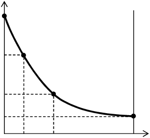
Refer to caption β max β min z 0 z 1 z 2 z 3 β z ( β ) Refer to caption s 0 s 1 s 2 s 3 z 0 z 1 z 2 z 3 s ( β ) z ( β ) - + + Refer to caption s η + s
(a)         (b)         (c)
Figure 1: (a) z⁡(β)=ln⁡Z⁡(β)z(\beta)=\ln Z(\beta) is a strictly convex decreasing function. Four dots show a possible output of Algorithm 4. Here ℓ=3\ell=3 and [β0,βℓ]=[βmin,βmax][\beta_{0},\beta_{\ell}]=[{\beta_{\min}},{\beta_{\max}}]. (b) Definitions of the sets Δi\Delta_{i} (in gray). Intervals 00 and 11 are assumed to be large, while interval 22 is small. (c) Definition of the variable ηs+\eta^{+}_{s} (in the case of a large interval).

By geometric considerations it should be clear that

A​r​e​a​(Δ−)≤max⁡{|zi−zi+1|:i is small}⋅|S|≤τ⋅1m⋅|S|Area(\Delta^{-})\;\;\leq\;\;\max\left\{|z_{i}-z_{i+1}|\>:\>\mbox{$i$ is small}\right\}\cdot|S|\;\;\leq\;\;\tau\cdot\mbox{$\frac{1}{m}$}\cdot|S|

Observe that −z′​(β)=𝔼X∼μβ​[H⁡(X)]∈[1,n]-z^{\prime}(\beta)={\mathbb{E}}_{X\sim\mu_{\beta}}[H(X)]\in[1,n] for any β\beta, and therefore S=[sℓ,s0]⊆[0,ln⁡n]S=[s_{\ell},s_{0}]\subseteq[0,\ln n] and so |S|≤ln⁡n|S|\leq\ln n. This establishes the first claim of Lemma 4. Next, we focus on proving the second claim.

For a point s∈Ss\in S let ηs\eta_{s} be the length of the interval (zi+1,zi)(z_{i+1},z_{i}) into which z⁡(s)z(s) falls (or 00, if z⁡(s)∈{zℓ,…,z0}z(s)\in\{z_{\ell},\ldots,z_{0}\}). Also let ηs+=ψ⁡[ηs]\eta^{+}_{s}=\psi[\eta_{s}] where ψ⁡[⋅]\psi[\cdot] is the following function: ψ⁡[a]=a\psi[a]=a if a>τ⋅1ma>\tau\cdot\frac{1}{m}, and ψ⁡[a]=0\psi[a]=0 otherwise. Thus, if z⁡(s)∈(zi+1,zi)z(s)\in(z_{i+1},z_{i}) for some large interval ii then ηs+=zi−zi+1\eta^{+}_{s}=z_{i}-z_{i+1} (Fig. 1(c)), otherwise ηs+=0\eta^{+}_{s}=0. We have

A​r​e​a​(Δ+)=∫Sηs+​𝑑sArea(\Delta^{+})=\int_{S}\eta^{+}_{s}ds

The linearity of expectation gives

2​𝔼​[δ+]\displaystyle 2{\mathbb{E}}[\delta^{+}] ≤\displaystyle\leq 𝔼⁡(A​r​e​a​(Δ+))=∫S𝔼⁡[ηs+]​𝑑s≤maxs∈S⁡𝔼⁡[ηs+]⋅|S|\displaystyle{\mathbb{E}}(Area(\Delta^{+}))\;\;=\;\;\int_{S}{\mathbb{E}}[\eta^{+}_{s}]ds\;\;\leq\;\;\max_{s\in S}{\mathbb{E}}[\eta^{+}_{s}]\cdot|S| (11)

Now let X0,X1,X2,…X_{0},X_{1},X_{2},\ldots be a Poisson process on [0,+∞)[0,+\infty) and X−1,X−2,…X_{-1},X_{-2},\ldots be a Poisson process on (−∞,0](-\infty,0] (both with rate kk). Thus, Xi=ξ0+…+ξiX_{i}=\xi_{0}+\ldots+\xi_{i} for i≥0i\geq 0 and Xi=−ξ−1−ξ−2−…−ξiX_{i}=-\xi_{-1}-\xi_{-2}-\ldots-\xi_{i} for i≤−1i\leq-1, where ξj\xi_{j} are i.i.d. variables from the exponential distribution of rate kk. By the superposition theorem for Poisson processes [15, page 16], bidirectional sequence 𝐗=…,X−2,X−1,X0,X1,X2,…{\bf X}=\ldots,X_{-2},X_{-1},X_{0},X_{1},X_{2},\ldots is a Poisson process on (−∞,+∞)(-\infty,+\infty) (again with rate kk), and in particular it is translation-invariant.

Let 𝐘=…,Y−2,Y−1,Y0,Y1,Y2,…{\bf Y}=\ldots,Y_{-2},Y_{-1},Y_{0},Y_{1},Y_{2},\ldots be the following process: draw an integer c∈{0,…,d−1}c\in\mbox{$\{0,\ldots,d-1\}$} uniformly at random and then set Yi=Xd​i+cY_{i}=X_{di+c} for each ii. It can be seen that 𝐘{\bf Y} models the output (β0,…,βℓ)(\beta_{0},\ldots,\beta_{\ell}) of Algorithm 4 as follows: take the sequence z⁡(βmin)−Y0,z⁡(βmin)−Y1,z⁡(βmin)−Y2,…z({\beta_{\min}})-Y_{0},z({\beta_{\min}})-Y_{1},z({\beta_{\min}})-Y_{2},\ldots, restrict to [z⁡(βmax),z⁡(βmin)][z({\beta_{\max}}),z({\beta_{\min}})] and append z⁡(βmin)z({\beta_{\min}}) and z⁡(βmax)z({\beta_{\max}}). Then the resulting sequence has the same distribution as (z⁡(β0),…,z⁡(βℓ))(z(\beta_{0}),\ldots,z(\beta_{\ell})). We assume below that (β0,…,βℓ)(\beta_{0},\ldots,\beta_{\ell}) is generated by this procedure.

For a point a∈ℝa\in\mathbb{R} let θa\theta_{a} be the length of the interval (Yi,Yi+1)(Y_{i},Y_{i+1}) into which aa falls (or 00, if no such interval exists). Note, the distribution of random variable θa\theta_{a} does not depend on aa (since process 𝐘{\bf Y} is translation-invariant). We also denote θa+=ψ⁡[θa]\theta^{+}_{a}=\psi[\theta_{a}], and let θ\theta and θ+=ψ⁡[θ]\theta^{+}=\psi[\theta] be random variables with the same distributions as θa\theta_{a} and θa+\theta^{+}_{a}, respectively (for any fixed aa). Clearly, for each s∈[sℓ,s0]s\in[s_{\ell},s_{0}] we have ηs≤θa\eta_{s}\leq\theta_{a} and ηs+≤θa+\eta^{+}_{s}\leq\theta^{+}_{a} for a suitably chosen aa, namely, a=z⁡(βmin)−z⁡(s)a=z({\beta_{\min}})-z(s). (Note, if z⁡(s)∈(zℓ−1,z1)z(s)\in(z_{\ell-1},z_{1}) then ηs=θa\eta_{s}=\theta_{a} and ηs+=θa+\eta^{+}_{s}=\theta^{+}_{a}, but at the boundaries the inequalities may be strict). We thus have

𝔼⁡[ηs+]≤𝔼⁡[θ+]{\mathbb{E}}[\eta^{+}_{s}]\leq{\mathbb{E}}[\theta^{+}] (12)
Lemma 10.

Variable θ\theta has the gamma (Erlang) distribution with shape parameter d+1d+1 and rate kk, whose probability density is f⁡(t)=kd+1​td​e−k​t/d!f(t)=k^{d+1}t^{d}e^{-kt}/d! for t≥0t\geq 0.

Proof.

We prove this fact for variable θa\theta_{a} with a=0a=0. We know that Y−1=Xc−d≤0Y_{-1}=X_{c-d}\leq 0 and Y0=Xc≥0Y_{0}=X_{c}\geq 0, so θ0=Y0−Y−1\theta_{0}=Y_{0}-Y_{-1} (with probability 1). By construction, Xc−Xc−d=ξc−d+ξc−d+1+…+ξcX_{c}-X_{c-d}=\xi_{c-d}+\xi_{c-d+1}+\ldots+\xi_{c}, i.e. θ0\theta_{0} is a sum of d+1d+1 i.i.d. exponential random variables each of rate kk. This implies the claim. ∎

Remark 2.

It may seem counterintuitive that all intervals ζi=Yi−Yi−1\zeta_{i}=Y_{i}-Y_{i-1} are distributed as a sum of dd exponential random variables with the exception of i=0i=0, in which case it is a sum of d+1d+1 variables (even though 𝐘{\bf Y} is translation-invariant). This can be viewed as an instance of the “inspection paradox”, discussed e.g. at [1]. Below we describe an alternative approach, which may help to understand this phenomenon.

Let ζ\zeta be a sum of dd exponential random variables each of rate kk and g⁡(⋅)g(\cdot) be the probability density of ζ\zeta. Then the following (non-rigorous) argument shows that the probability density of θ\theta is t​g​(t)/𝔼⁡[ζ]tg(t)/{\mathbb{E}}[\zeta] (after which a simple calculation would prove the claim).

Let LL be some large number. Since the distribution of θa\theta_{a} does not depend on aa, we can define θ\theta as the output of the following process: sample 𝐘{\bf Y}, sample a∈[0,L]a\in[0,L] uniformly at random, and then set θ=θa\theta=\theta_{a} (i.e. the length of the interval in 𝐘{\bf Y} into which aa falls). Let us compute the probability that θ∈[t,t+d​t]\theta\in[t,t+dt]. Process 𝐘{\bf Y} will have L/𝔼⁡[ζ]L/{\mathbb{E}}[\zeta] intervals in [0,L][0,L] on average, and out of those (L/𝔼⁡[ζ])⋅(g⁡(t)​d​t)(L/{\mathbb{E}}[\zeta])\cdot(g(t)dt) intervals will have length in the range [t,t+d​t][t,t+dt]. The combined length of such intervals is (L/𝔼⁡[ζ])⋅(g⁡(t)​d​t)⋅t(L/{\mathbb{E}}[\zeta])\cdot(g(t)dt)\cdot t. Thus, point aa will fall into one of those intervals with probability (L/𝔼⁡[ζ])⋅(g⁡(t)​d​t)⋅t/L=(t​g​(t)/𝔼⁡[ζ])​d​t(L/{\mathbb{E}}[\zeta])\cdot(g(t)dt)\cdot t/L=(tg(t)/{\mathbb{E}}[\zeta])dt. Therefore, the density of θ\theta is t​g​(t)​d​t/𝔼⁡[ζ]tg(t)dt/{\mathbb{E}}[\zeta].

Recall that θ+=θ\theta^{+}=\theta if θ>τ/m\theta>\tau/m, and θ+=0\theta^{+}=0 otherwise. Lemma 10 now gives

𝔼⁡[θ+]\displaystyle{\mathbb{E}}[\theta^{+}] =\displaystyle= ∫τ/m+∞t​f​(t)​𝑑t=∫τ/m+∞kd+1​td+1​e−k​td!​𝑑t=∫τ​d/k+∞(k​t)d+1​e−(k​t)k⋅d!​d​(k​t)\displaystyle\int\limits_{\tau/m}^{+\infty}tf(t)dt\;\;=\;\;\int\limits_{\tau/m}^{+\infty}\frac{k^{d+1}t^{d+1}e^{-kt}}{d!}dt\;\;=\;\;\int\limits_{\tau d/k}^{+\infty}\frac{(kt)^{d+1}e^{-(kt)}}{k\cdot d!}d(kt)
=\displaystyle= 1k⋅d!​∫τ​d+∞ud+1​e−u​𝑑u=Γ⁡(d+2,τ​d)k⋅d!=Γ⁡(d+2,τ​d)m​d⋅d!\displaystyle\frac{1}{k\cdot d!}\int\limits_{\tau d}^{+\infty}u^{d+1}\,e^{-u}du\;\;=\;\;\frac{\Gamma(d+2,\tau d)}{k\cdot d!}\;\;=\;\;\frac{\Gamma(d+2,\tau d)}{md\cdot d!}

Combining this with (11) and (12) and observing again that |S|≤ln⁡n|S|\leq\ln n finally gives the second claim of Lemma 4.

4.2 Proof of Lemma 6

We will use the same notation as in the previous section. Since H⁡(⋅)H(\cdot) can now take value 00, we have −z′​(β)=𝔼X∼μβ​[H⁡(X)]∈[0,n]-z^{\prime}(\beta)={\mathbb{E}}_{X\sim\mu_{\beta}}[H(X)]\in[0,n] and so [sℓ,s0]⊆[−∞,ln⁡n][s_{\ell},s_{0}]\subseteq[-\infty,\ln n] (instead of [sℓ,s0]⊆[0,ln⁡n][s_{\ell},s_{0}]\subseteq[0,\ln n], as in the previous section). We will deal with small values of s⁡(β)s(\beta) exactly as in [9].

Recall that z′​(β)z^{\prime}(\beta) is a strictly increasing function of β\beta. Let β^\hat{\beta} be the unique value with z′​(β^)=−λz^{\prime}(\hat{\beta})=-\lambda. (If it does not exist, then we take β^∈{−∞,+∞}\hat{\beta}\in\{-\infty,+\infty\} using the natural rule). Denote z^=z⁡(β^)\hat{z}=z(\hat{\beta}) and s^=ln⁡[−z′​(β^)]\hat{s}=\ln[-z^{\prime}(\hat{\beta})]. Now introduce the following terminology for an interval i∈[0,ℓ−1]i\in[0,\ell-1]:

  • •

    interval ii is steep if βi+1≤β^\beta_{i+1}\leq\hat{\beta}, or equivalently si+1≥s^s_{i+1}\geq\hat{s};

  • •

    interval ii is flat if βi≥β^\beta_{i}\geq\hat{\beta}, or equivalently si≤s^s_{i}\leq\hat{s};

  • •

    interval ii is crossing if β^∈(βi,βi+1)\hat{\beta}\in(\beta_{i},\beta_{i+1}), or equivalently s^∈(si+1,si)\hat{s}\in(s_{i+1},s_{i}).

If steep intervals exist then β^≥βmin\hat{\beta}\geq{\beta_{\min}} and z′​(β^)≤−λz^{\prime}(\hat{\beta})\leq-\lambda. (The inequality may be strict if β^=+∞\hat{\beta}=+\infty). We thus have [si+1,si]⊆[s^,s0]⊆[ln⁡λ,ln⁡n][s_{i+1},s_{i}]\subseteq[\hat{s},s_{0}]\subseteq[\ln\lambda,\ln n] for all steep intervals ii. The argument from the previous section gives that

∑i: i is steep and smallδi≤τ2⋅ln⁡nλm𝔼[∑i: i is steep and largeδi]≤Γ⁡(d+2,τ​d)2​d⋅d!⋅ln⁡nλm\sum_{\mbox{\small$i$: $i$ is steep and small}}\delta_{i}\leq\frac{\tau}{2}\cdot\frac{\ln\frac{n}{\lambda}}{m}\hskip 20.00003pt\hskip 20.00003pt{\mathbb{E}}\left[\sum_{\mbox{\small$i$: $i$ is steep and large}}\delta_{i}\right]\leq\frac{\Gamma(d+2,\tau d)}{2d\;\cdot\;d!}\cdot\frac{\ln\frac{n}{\lambda}}{m}

(We just need to assume that βmax{\beta_{\max}} was replaced with min⁡{βmax,β^}\min\{{\beta_{\max}},\hat{\beta}\}, then we would have S=[sℓ,s0]⊆[ln⁡λ,ln⁡n]S=[s_{\ell},s_{0}]\subseteq[\ln\lambda,\ln n] and |S|≤ln⁡nλ|S|\leq\ln\frac{n}{\lambda} instead of |S|≤ln⁡n|S|\leq\ln n, the rest is the same as in the previous section).

Let us now consider flat intervals. The argument from [9] gives the following fact.

Lemma 11.

The sum of δi\delta_{i} over flat intervals ii is at most ln⁡11−λ\ln\frac{1}{1-\lambda}.

Proof.

Assume that flat intervals exist, then β^≤βmax\hat{\beta}\leq{\beta_{\max}} and z′​(β^)≥−λz^{\prime}(\hat{\beta})\geq-\lambda. (The inequality may be strict if β^=−∞\hat{\beta}=-\infty). Denote Ω0={x∈Ω|H⁡(x)=0}\Omega_{0}=\{x\in\Omega\>|\>H(x)=0\} and Ω+={x∈Ω|H⁡(x)≥1}\Omega_{+}=\{x\in\Omega\>|\>H(x)\geq 1\}, then Ω=Ω0∪Ω+\Omega=\Omega_{0}\cup\Omega_{+} and

𝔼X∼μβ^​[H⁡(X)]=∑x∈Ω+H⁡(x)​e−β^​H​(x)Z⁡(β^)≥∑x∈Ω+e−β^​H​(x)Z⁡(β^)=1−∑x∈Ω0e−β^​H​(x)Z⁡(β^)≥1−Z⁡(βmax)Z⁡(β^){\mathbb{E}}_{X\sim\mu_{\hat{\beta}}}[H(X)]=\frac{\sum_{x\in\Omega_{+}}\;\;H(x)e^{-\hat{\beta}H(x)}}{Z(\hat{\beta})}\geq\frac{\sum_{x\in\Omega_{+}}\;\;e^{-\hat{\beta}H(x)}}{Z(\hat{\beta})}=1-\frac{\sum_{x\in\Omega_{0}}\;\;e^{-\hat{\beta}H(x)}}{Z(\hat{\beta})}\geq 1-\frac{Z({\beta_{\max}})}{Z(\hat{\beta})}

On the other hand, 𝔼X∼μβ^​[H⁡(X)]=−z′​(β^)≤λ{\mathbb{E}}_{X\sim\mu_{\hat{\beta}}}[H(X)]=-z^{\prime}(\hat{\beta})\leq\lambda and so Z⁡(βmax)Z⁡(β^)≥1−λ\frac{Z({\beta_{\max}})}{Z(\hat{\beta})}\geq 1-\lambda and z⁡(β^)−z⁡(βmax)≤ln⁡11−λz(\hat{\beta})-z({\beta_{\max}})\leq\ln\frac{1}{1-\lambda}. For all flat intervals ii we have [zi+1,zi]⊆[z⁡(βmax),z⁡(β^)][z_{i+1},z_{i}]\subseteq[z({\beta_{\max}}),z(\hat{\beta})] and also δi≤zi−zi+1\delta_{i}\leq z_{i}-z_{i+1}. This gives the claim of the lemma. ∎

It remains to consider crossing intervals. Let us define values δc−\delta_{c}^{-} and δc+\delta_{c}^{+} as follows. If there are no crossing intervals then δc−=δc+=0\delta_{c}^{-}=\delta_{c}^{+}=0. Otherwise let ii be the unique crossing interval; if ii is small then set (δc−,δc+)=(δi,0)(\delta_{c}^{-},\delta_{c}^{+})=(\delta_{i},0), and if ii is large then set (δc−,δc+)=(0,δi)(\delta_{c}^{-},\delta_{c}^{+})=(0,\delta_{i}). In all cases we have δc−≤τm\delta_{c}^{-}\leq\frac{\tau}{m} (since δi≤zi−zi+1\delta_{i}\leq z_{i}-z_{i+1}). Also, 𝔼⁡[δc+]≤𝔼⁡[ψ⁡(zi−zi+1)]≤𝔼⁡[θ+]≤Γ⁡(d+2,τ​d)m​d⋅d!{\mathbb{E}}[\delta_{c}^{+}]\leq{\mathbb{E}}[\psi(z_{i}-z_{i+1})]\leq{\mathbb{E}}[\theta^{+}]\leq\frac{\Gamma(d+2,\tau d)}{md\;\cdot\;d!} where function ψ⁡(⋅)\psi(\cdot) and random variable θ+\theta^{+} were defined in the previous section.

We can finally prove Lemma 6. Define δ−\delta^{-} as δc−\delta_{c}^{-} plus the sum of δi\delta_{i} over small steep intervals ii and flat intervals ii. Define δ+\delta^{+} as δc+\delta_{c}^{+} plus the sum of δi\delta_{i} over large steep intervals ii. By collecting inequalities above we obtain the desired claim.

5 Lower bound

In this section we establish a lower bound on the number of calls to the sampling oracles for estimating q=ln⁡Z⁡(βmin)Z⁡(βmax)q=\ln\frac{Z({\beta_{\min}})}{Z({\beta_{\max}})}. First, we describe our model of computation and the set of instances that we allow.

We assume that the estimation algorithm only receives values H⁡(x)H(x) from the sampling oracle, and not individual states x∈Ωx\in\Omega. This means that an instance can be defined by counts ch=|{x∈Ω|H⁡(x)=h}|c_{h}=|\{x\in\Omega\>|\>H(x)=h\}| for values hh in the range of HH; these counts uniquely specify the partition function Z⁡(β)=∑hch​e−β​hZ(\beta)=\sum_{h}c_{h}e^{-\beta h} and the distribution of sampling oracle outputs for a given β\beta. We will thus view an instance as a triplet Γ=(c⁡[Γ],βmin​[Γ],βmax​[Γ])\Gamma=(c[\Gamma],{\beta_{\min}}[\Gamma],{\beta_{\max}}[\Gamma]) where c⁡[Γ]:ℝ→ℤ≥0c[\Gamma]:\mathbb{R}\rightarrow\mathbb{Z}_{\geq 0} is a function with a finite non-empty support. When the instance is clear from the context, we will omit the square brackets and write simply Γ=(c,βmin,βmax)\Gamma=(c,{\beta_{\min}},{\beta_{\max}}). For a value h∈𝚜𝚞𝚙𝚙⁡(c)h\in{\tt supp}(c) let ψ⁡(β,h|Γ)\psi(\beta,h\>|\>\Gamma) be the probability that the sampling oracle returns value hh when queried at β\beta in instance Γ\Gamma:

ψ⁡(β,h|Γ)=ch​e−β​h/Z⁡(β)\psi(\beta,h\>|\>\Gamma)=c_{h}e^{-\beta h}/Z(\beta)

For a finite subset ℋ⊆ℝ{\cal H}\subseteq\mathbb{R} let 𝕀⁡(ℋ)\mathbb{I}({\cal H}) be the set of instances Γ=(c,0,βmax)\Gamma=(c,0,{\beta_{\max}}) satisfying 𝚜𝚞𝚙𝚙⁡(c)⊆ℋ{\tt supp}(c)\subseteq{\cal H}. Also for a subset 𝒬⊆ℝ{\cal Q}\subseteq\mathbb{R} let 𝕀⁡(ℋ,𝒬)={Γ∈𝕀⁡(ℋ)|q∗​(Γ)∈𝒬}\mathbb{I}({\cal H},{\cal Q})=\{\Gamma\in\mathbb{I}({\cal H})\>|\>q^{\ast}(\Gamma)\in{\cal Q}\}, where we denoted q∗​(Γ)=ln⁡Z⁡(0)Z⁡(βmax)q^{\ast}(\Gamma)=\ln\frac{Z(0)}{Z({\beta_{\max}})}.

An estimation algorithm 𝒜{\cal A} applied to instance Γ=(c,0,βmax)∈𝕀⁡(ℋ)\Gamma=(c,0,{\beta_{\max}})\in\mathbb{I}({\cal H}) is assumed to have the following form. At step ii (for i=1,2,…i=1,2,\ldots) it does one of the following two actions:

  1. 1.

    Call the samping oracle for some value βi∈ℝ\beta_{i}\in\mathbb{R}. The oracle then returns a random variable hi∈ℋh_{i}\in{\cal H} with ℙ⁡(hi=h)=ψ⁡(βi,h|Γ){\mathbb{P}}(h_{i}=h)=\psi(\beta_{i},h\>|\>\Gamma) for each h∈ℋh\in{\cal H}.

  2. 2.

    Output some estimate q^\hat{q} and terminate.

The ii-th action is a random variable that can depend only on the set 𝚜𝚞𝚙𝚙⁡(c){\tt supp}(c), values βmin,βmax{\beta_{\min}},{\beta_{\max}}, and on the previously observed sequence (β1,h1),…,(βi−1,hi−1)(\beta_{1},h_{1}),\ldots,(\beta_{i-1},h_{i-1}). The output q^\hat{q} of the algorithm will be denoted as q𝒜​(Γ)q^{{\cal A}}(\Gamma), and the expected number of calls to the sampling oracle as T𝒜​(Γ)T^{{\cal A}}(\Gamma).

We say that algorithm 𝒜{\cal A} is an (ε,δ)(\varepsilon,\delta)-estimator for instance Γ\Gamma if ℙ[|q𝒜(Γ)−q∗(Γ)|>ε]<δ{\mathbb{P}}[|q^{{\cal A}}(\Gamma)-q^{\ast}(\Gamma)|>\varepsilon]<\delta. We can now formulate our main theorem.

Theorem 12.

There exist positive numbers qmin,nmin,c1,c2,c3q_{\min},n_{\min},c_{1},c_{2},c_{3} such that the following holds for all q≥qminq\geq q_{\min}, n≥nminn\geq n_{\min} with n∈ℤn\in\mathbb{Z}, ε∈(0,c1​q)\varepsilon\in(0,c_{1}q), δ∈(0,14)\delta\in(0,\frac{1}{4}).

Denote m=⌈c2​qn⌉m=\left\lceil\frac{c_{2}\sqrt{q}}{n}\right\rceil and ℋnm={h∈[1,n]:m​h∈ℤ}{\cal H}_{n}^{m}=\{h\in[1,n]\>:\>mh\in\mathbb{Z}\}. Suppose that 𝒜{\cal A} is an (ε,δ)(\varepsilon,\delta)-estimator for all instances in 𝕀⁡(ℋnm,[2​q3,4​q3])\mathbb{I}({\cal H}_{n}^{m},\left[\frac{2q}{3},\frac{4q}{3}\right]). Then there exists instance Γ∈𝕀⁡(ℋnm,[2​q3,4​q3])\Gamma\in\mathbb{I}({\cal H}_{n}^{m},\left[\frac{2q}{3},\frac{4q}{3}\right]) such that T𝒜​(Γ)≥c3​q​ε−2​ln⁡δ−1T^{\cal A}(\Gamma)\geq c_{3}q\varepsilon^{-2}\ln\delta^{-1}.

5.1 Proof of Theorem 12

The proof will be based on the following result. For brevity, we use notation a±ba\pm b to denote the closed interval [a−b,a+b][a-b,a+b].

Lemma 13.

Suppose that 𝒜{\cal A} is an (ε,δ)(\varepsilon,\delta)-estimator for instances Γ∈𝕀⁡(ℋ,{q})\Gamma\in\mathbb{I}({\cal H},\{q\}) and Γ1,…,Γd∈𝕀⁡(ℋ,ℝ∖(q±2​ε))\Gamma_{1},\ldots,\Gamma_{d}\in\mathbb{I}({\cal H},\mathbb{R}\setminus(q\pm 2\varepsilon)), where βmax​[Γi]=βmax​[Γ]{\beta_{\max}}[\Gamma_{i}]={\beta_{\max}}[\Gamma] and 𝚜𝚞𝚙𝚙⁡(c⁡[Γi])=𝚜𝚞𝚙𝚙⁡(c⁡[Γ]){\tt supp}(c[\Gamma_{i}])={\tt supp}(c[\Gamma]) for i∈[d]i\in[d]. Suppose that

∏i∈[d]ψ⁡(β,h|Γi)ψ⁡(β,h|Γ)≥γ∀β∈ℝ,h∈𝚜𝚞𝚙𝚙⁡(c⁡[Γ])\prod_{i\in[d]}\frac{\psi(\beta,h\>|\>\Gamma_{i})}{\psi(\beta,h\>|\>\Gamma)}\geq\gamma\hskip 20.00003pt\hskip 10.00002pt\forall\beta\in\mathbb{R},h\in{\tt supp}(c[\Gamma]) (13)

for some constant γ∈(0,1)\gamma\in(0,1). Then T𝒜​(Γ)≥(1−δ′−δ)​d​ln⁡(δ′/δ)ln⁡(1/γ)T^{\cal A}(\Gamma)\geq\frac{(1-\delta^{\prime}-\delta)d\ln(\delta^{\prime}/\delta)}{\ln(1/\gamma)} for any constant δ′∈[δ,1−δ]\delta^{\prime}\in[\delta,1-\delta].

Proof.

The run of the algorithm can be described by a random variable X=((β1,h1),…,(βt,ht),q^)X=((\beta_{1},h_{1}),\ldots,(\beta_{t},h_{t}),\hat{q}), where tt is the number of oracle calls (possibly infinite, in which case q^\hat{q} is undefined). Let 𝒳{\cal X} be the set all possible runs, and ℙ𝒜(⋅|Γ~){\mathbb{P}}^{\cal A}(\cdot\>|\>\tilde{\Gamma}) be the probability measure of this random variable conditioned on Γ~\tilde{\Gamma} being the input instance. The structure of the algorithm implies that this measure can be decomposed as follows:

d​ℙ𝒜​(x|Γ~)=ψ⁡(x|Γ~)​d​μ𝒜​(x)∀x∈{((β1,h1),…,(βt,ht),q^)∈𝒳|t is finite}d{\mathbb{P}}^{\cal A}(x\>|\>\tilde{\Gamma})=\psi(x\>|\>\tilde{\Gamma})\>d\mu^{\cal A}(x)\hskip 20.00003pt\forall x\in\{((\beta_{1},h_{1}),\ldots,(\beta_{t},h_{t}),\hat{q})\in{\cal X}\>|\>\mbox{$t$ is finite}\} (14)

where μ𝒜​(⋅)\mu^{\cal A}(\cdot) is some measure on 𝒳{\cal X} that depends only on the algorithm 𝒜{\cal A}, and function ψ⁡(⋅)\psi(\cdot) is defined via

ψ⁡((β1,h1),…,(βt,ht),q^|Γ~)=∏i∈[t]ψ⁡(βi,hi|Γ~)\psi((\beta_{1},h_{1}),\ldots,(\beta_{t},h_{t}),\hat{q}\>|\>\tilde{\Gamma})=\prod_{i\in[t]}\psi(\beta_{i},h_{i}\>|\>\tilde{\Gamma})

Denote τ=d​ln⁡(δ′/δ)ln⁡(1/γ)\tau=\frac{d\ln(\delta^{\prime}/\delta)}{\ln(1/\gamma)}, and define the following subsets of 𝒳{\cal X}:

𝒳∗\displaystyle{\cal X}^{\ast} =\displaystyle= {((β1,h1),…,(βt,ht),q^)∈𝒳|t≤τ and q^∈q±ε }\displaystyle\{((\beta_{1},h_{1}),\ldots,(\beta_{t},h_{t}),\hat{q})\in{\cal X}\>\>|\>\>\mbox{$t\leq\tau$ and $\hat{q}\in q\pm\varepsilon$ }\}
𝒳′\displaystyle{\cal X}^{\prime} =\displaystyle= {((β1,h1),…,(βt,ht),q^)∈𝒳|t>τ }\displaystyle\{((\beta_{1},h_{1}),\ldots,(\beta_{t},h_{t}),\hat{q})\in{\cal X}\>\>|\>\>\mbox{$t>\tau$ }\}
𝒳′′\displaystyle{\cal X}^{\prime\prime} =\displaystyle= {((β1,h1),…,(βt,ht),q^)∈𝒳|t≤τ and q^∉q±ε }\displaystyle\{((\beta_{1},h_{1}),\ldots,(\beta_{t},h_{t}),\hat{q})\in{\cal X}\>\>|\>\>\mbox{$t\leq\tau$ and $\hat{q}\notin q\pm\varepsilon$ }\}

Suppose the claim of Lemma 13 is false, i.e. T𝒜​(Γ)≤(1−δ′−δ)⋅τT^{\cal A}(\Gamma)\leq(1-\delta^{\prime}-\delta)\cdot\tau. We have T𝒜​(Γ)≥ℙ𝒜​(𝒳′|Γ)⋅τT^{\cal A}(\Gamma)\geq{\mathbb{P}}^{\cal A}({\cal X}^{\prime}\>|\>\Gamma)\cdot\tau, and therefore

ℙ𝒜​(𝒳′|Γ)\displaystyle{\mathbb{P}}^{\cal A}({\cal X}^{\prime}\>|\>\Gamma) ≤\displaystyle\leq 1−δ−δ′\displaystyle 1-\delta-\delta^{\prime}\hskip 20.00003pt\hskip 20.00003pt (15)

Since 𝒜{\cal A} is a (ε,δ)(\varepsilon,\delta)-estimator for instances Γ,Γ1,…,Γd\Gamma,\Gamma_{1},\ldots,\Gamma_{d}, we have

ℙ𝒜​(𝒳′′|Γ)\displaystyle{\mathbb{P}}^{\cal A}({\cal X}^{\prime\prime}\>|\>\Gamma)~ <\displaystyle< δ\displaystyle\delta (16)
ℙ𝒜​(𝒳∗|Γi)\displaystyle{\mathbb{P}}^{\cal A}({\cal X}^{\ast}\>|\>\Gamma_{i}) <\displaystyle< δ∀i∈[d]\displaystyle\delta\hskip 20.00003pt\hskip 20.00003pt\forall i\in[d] (17)

Set 𝒳{\cal X} is a disjoint union of 𝒳∗,𝒳′,𝒳′′{\cal X}^{\ast},{\cal X}^{\prime},{\cal X}^{\prime\prime}, therefore ℙ𝒜​(𝒳∗|Γ)=1−ℙ𝒜​(𝒳′|Γ)−ℙ𝒜​(𝒳′′|Γ)>1−(1−δ−δ′)−δ=δ′{\mathbb{P}}^{\cal A}({\cal X}^{\ast}\>|\>\Gamma)=1-{\mathbb{P}}^{\cal A}({\cal X}^{\prime}\>|\>\Gamma)-{\mathbb{P}}^{\cal A}({\cal X}^{\prime\prime}\>|\>\Gamma)>1-(1-\delta-\delta^{\prime})-\delta=\delta^{\prime}. Combining this with (17) gives

1d​∑i∈[d]ℙ𝒜​(𝒳∗|Γi)\displaystyle\frac{1}{d}\sum_{i\in[d]}{\mathbb{P}}^{\cal A}({\cal X}^{\ast}\>|\>\Gamma_{i}) <\displaystyle< δδ′​ℙ𝒜​(𝒳∗|Γ)\displaystyle\frac{\delta}{\delta^{\prime}}\>{\mathbb{P}}^{\cal A}({\cal X}^{\ast}\>|\>\Gamma) (18)

Assumption (13) of the lemma gives that

∏i∈[d]ψ⁡(x|Γi)ψ⁡(x|Γ)≥γt≥γτ∀x=((β1,h1),…,(βt,ht),q^)∈𝒳∗\prod_{i\in[d]}\frac{\psi(x\>|\>\Gamma_{i})}{\psi(x\>|\>\Gamma)}\;\;\geq\;\;\gamma^{t}\;\;\geq\;\;\gamma^{\tau}\hskip 20.00003pt\hskip 10.00002pt\forall x=((\beta_{1},h_{1}),\ldots,(\beta_{t},h_{t}),\hat{q})\in{\cal X}^{\ast} (19)

We can now write

1d​∑i∈[d]ψ⁡(x|Γi)≥(∏i∈[d]ψ⁡(x|Γi))1/d≥γτ/d​ψ​(x|Γ)=δδ′​ψ​(x|Γ)∀x∈𝒳∗\frac{1}{d}\sum_{i\in[d]}\psi(x\>|\>\Gamma_{i})\;\geq\;\left(\prod_{i\in[d]}\psi(x\>|\>\Gamma_{i})\right)^{1/d}\;\geq\;\gamma^{\tau/d}\psi(x\>|\>\Gamma)\;=\;\frac{\delta}{\delta^{\prime}}\>\psi(x\>|\>\Gamma)\hskip 20.00003pt\hskip 10.00002pt\forall x\in{\cal X}^{\ast} (20)

where the first inequality is a relation between arithmetic and geometric means of non-negative numbers, and the second inequality follows from (19). We can write

1d​∑i∈[d]ℙ𝒜​(𝒳∗|Γi)=(a)1d​∑i∈[d]∫𝒳∗ψ⁡(x|Γi)​d​μ𝒜​(x)≥(b)δδ′​∫𝒳∗ψ⁡(x|Γ)​d​μ𝒜​(x)=(c)δδ′​ℙ𝒜​(𝒳∗|Γ)\frac{1}{d}\sum_{i\in[d]}{\mathbb{P}}^{\cal A}({\cal X}^{\ast}\>|\>\Gamma_{i})\;\stackrel{{\scriptstyle\mbox{\tiny(a)}}}{{=}}\;\frac{1}{d}\sum_{i\in[d]}\int_{{\cal X}^{\ast}}\psi(x\>|\>\Gamma_{i})\>d\mu^{\cal A}(x)\;\stackrel{{\scriptstyle\mbox{\tiny(b)}}}{{\geq}}\;\frac{\delta}{\delta^{\prime}}\int_{{\cal X}^{\ast}}\psi(x\>|\>\Gamma)\>d\mu^{\cal A}(x)\;\stackrel{{\scriptstyle\mbox{\tiny(c)}}}{{=}}\;\frac{\delta}{\delta^{\prime}}\>{\mathbb{P}}^{\cal A}({\cal X}^{\ast}\>|\>\Gamma)

where (a,c) follow from (14) and (b) follows from (20). We obtained a contradiction to (18).

∎

Recall that by definition coefficients of instances should be non-negative integers. When using Lemma 13, we can relax this requirement to non-negative rationals (since multiplying coefficients by a constant does not affect quantities in Lemma 13) and further to non-negative reals (since they can be approximated by rationals with an arbitrary precision).

We will use Lemma 13 with d=2d=2 and three instances Γ,Γ+,Γ−\Gamma,\Gamma_{+},\Gamma_{-}. First, we will describe the construction of Γ+\Gamma_{+} and Γ−\Gamma_{-} given an instance Γ\Gamma. After stating some properties of this construction, we will define the instance Γ\Gamma.

Instances Γ+\Gamma_{+} and Γ−\Gamma_{-}   Suppose that Γ=(c,0,βmax)∈𝕀⁡(ℋ)\Gamma=(c,0,{\beta_{\max}})\in\mathbb{I}({\cal H}). We set Γ+=(c+,0,βmax)\Gamma_{+}=(c^{+},0,{\beta_{\max}}) and Γ−=(c−,0,βmax)\Gamma_{-}=(c^{-},0,{\beta_{\max}}) where functions c+,c−c^{+},c^{-} are given by

ch+=ch⋅eh​ν,ch−=ch⋅e−h​ν∀h∈ℝ\displaystyle c^{+}_{h}=c_{h}\cdot e^{h\nu},\hskip 20.00003ptc^{-}_{h}=c_{h}\cdot e^{-h\nu}\hskip 20.00003pt\hskip 20.00003pt\forall h\in\mathbb{R}

where ν>0\nu>0 is some constant. Let Z⁡(⋅)Z(\cdot), Z+​(⋅)Z_{+}(\cdot), Z−​(⋅)Z_{-}(\cdot) be the partition functions corresponding to Γ\Gamma, Γ+\Gamma_{+}, Γ−\Gamma_{-}, respectively. One can check that

Z⁡(β)=∑h∈𝚜𝚞𝚙𝚙⁡(c)ch​e−β​hZ+​(β)=Z⁡(β−ν)Z−​(β)=Z⁡(β+ν)Z(\beta)=\sum_{h\in{\tt supp}(c)}c_{h}e^{-\beta h}\hskip 20.00003ptZ_{+}(\beta)=Z(\beta-\nu)\hskip 20.00003ptZ_{-}(\beta)=Z(\beta+\nu)

Denote z⁡(β)=ln⁡Z⁡(β)z(\beta)=\ln Z(\beta) and z𝚍𝚒𝚏𝚏​(β)=z⁡(β)−z⁡(βmax+β)z_{\tt diff}(\beta)=z(\beta)-z({\beta_{\max}}+\beta). Then

q=q∗​[Γ]=z𝚍𝚒𝚏𝚏​(0)q∗​[Γ+]=z𝚍𝚒𝚏𝚏​(−ν)q∗​[Γ−]=z𝚍𝚒𝚏𝚏​(ν)q=q^{\ast}[\Gamma]=z_{\tt diff}(0)\hskip 20.00003ptq^{\ast}[\Gamma_{+}]=z_{\tt diff}(-\nu)\hskip 20.00003ptq^{\ast}[\Gamma_{-}]=z_{\tt diff}(\nu)

Condition Γ+,Γ−∈𝕀⁡(ℋ,ℝ∖(q±2​ε))\Gamma^{+},\Gamma^{-}\in\mathbb{I}({\cal H},\mathbb{R}\setminus(q\pm 2\varepsilon)) can thus be written as follows:

|z𝚍𝚒𝚏𝚏​(±ν)−z𝚍𝚒𝚏𝚏​(0)|>2​ε\displaystyle|z_{\tt diff}(\pm\nu)-z_{\tt diff}(0)|>2\varepsilon (21)

Condition (13) after cancellations becomes

Z2​(β)Z⁡(β−ν)​Z​(β+ν)≥γ∀β∈ℝ\frac{Z^{2}(\beta)}{Z(\beta-\nu)Z(\beta+\nu)}\geq\gamma\hskip 20.00003pt\hskip 10.00002pt\forall\beta\in\mathbb{R}

or equivalently

z⁡(β−ν)−2​z​(β)+z⁡(β+ν)≤ln⁡1γ∀β∈ℝ\displaystyle z(\beta-\nu)-2z(\beta)+z(\beta+\nu)\leq\ln\frac{1}{\gamma}\hskip 20.00003pt\hskip 10.00002pt\forall\beta\in\mathbb{R} (22)

Let us define the following quantities; note that they depend only on instance Γ\Gamma:

ρ=|z𝚍𝚒𝚏𝚏′​(0)|κ=supβ∈ℝz′′​(β)\rho=|z_{\tt diff}^{\prime}(0)|\hskip 20.00003pt\hskip 20.00003pt\kappa=\sup_{\beta\in\mathbb{R}}z^{\prime\prime}(\beta) (23)
Lemma 14.

Let Γ\Gamma be an instance with values q=q∗​(Γ),ρ,κq=q^{\ast}(\Gamma),\rho,\kappa as described above. Fix ε∈(0,ρ210​κ)\varepsilon\in(0,\frac{\rho^{2}}{10\kappa}). Suppose that algorithm 𝒜{\cal A} is an (ε,δ)(\varepsilon,\delta)-estimator for all instances in 𝕀⁡(ℋ,q±4​ε)\mathbb{I}({\cal H},q\pm 4\varepsilon). Then for any constant δ′∈[δ,1−δ]\delta^{\prime}\in[\delta,1-\delta] we have

T𝒜​(Γ)≥2​(1−δ′−δ)​ρ2​ln⁡(δ′/δ)9​κ​ε2T^{\cal A}(\Gamma)\geq\frac{2(1-\delta^{\prime}-\delta)\rho^{2}\ln(\delta^{\prime}/\delta)}{9\kappa\varepsilon^{2}}
Proof.

Non-negativity of function cc implies that function z⁡(⋅)z(\cdot) is convex, and so z′′​(β)∈[0,κ]z^{\prime\prime}(\beta)\in[0,\kappa] for all β∈ℝ\beta\in\mathbb{R}. Define ν=3​ε/ρ\nu=3\varepsilon/\rho. For β=±ν\beta=\pm\nu we can write

|z𝚍𝚒𝚏𝚏​(β)−z𝚍𝚒𝚏𝚏​(0)|=(a)|z𝚍𝚒𝚏𝚏′​(0)​β+z𝚍𝚒𝚏𝚏′′​(β~)​β22|∈(b)[|ρ​β|−κ​β2,|ρ​β|+κ​β2]|z_{\tt diff}(\beta)-z_{\tt diff}(0)|\;\stackrel{{\scriptstyle\mbox{\tiny(a)}}}{{=}}\;\left|z_{\tt diff}^{\prime}(0)\beta+z_{\tt diff}^{\prime\prime}(\tilde{\beta})\frac{\beta^{2}}{2}\right|\;\stackrel{{\scriptstyle\mbox{\tiny(b)}}}{{\in}}\;[|\rho\beta|-\kappa\beta^{2},|\rho\beta|+\kappa\beta^{2}]

where in (a) we used Taylor’s theorem with the Lagrange form of the remainder (here β~∈ℝ\tilde{\beta}\in\mathbb{R}), and in (b) we used the fact that |z𝚍𝚒𝚏𝚏′′​(β~)|=|z′′​(β~)−z′′​(βmax+β~)|≤2​κ|z_{\tt diff}^{\prime\prime}(\tilde{\beta})|=|z^{\prime\prime}(\tilde{\beta})-z^{\prime\prime}({\beta_{\max}}+\tilde{\beta})|\leq 2\kappa. Observing that |ρ​β|=3​ε|\rho\beta|=3\varepsilon and κ​β2=ε⋅9​κ​ερ2<ε\kappa\beta^{2}=\varepsilon\cdot\frac{9\kappa\varepsilon}{\rho^{2}}<\varepsilon, we get |z𝚍𝚒𝚏𝚏​(β)−z𝚍𝚒𝚏𝚏​(0)|∈(2​ε,4​ε)|z_{\tt diff}(\beta)-z_{\tt diff}(0)|\in(2\varepsilon,4\varepsilon). Thus, condition (21) holds, and Γ+,Γ−∈𝕀⁡(ℋ,q±4​ε)\Gamma_{+},\Gamma_{-}\in\mathbb{I}({\cal H},q\pm 4\varepsilon).

Denote f⁡(β)=z⁡(β)−z⁡(β−ν)f(\beta)=z(\beta)-z(\beta-\nu). Using twice the mean value theorem, we get

z⁡(β−ν)−2​z​(β)+z⁡(β+ν)=f⁡(β+ν)−f⁡(β)=f′​(β~)​ν=[z′​(β~)−z′​(β~−ν)]​ν=z′′​(β~~)​ν2≤κ​ν2z(\beta-\nu)-2z(\beta)+z(\beta+\nu)=f(\beta+\nu)-f(\beta)=f^{\prime}(\tilde{\beta})\nu=[z^{\prime}(\tilde{\beta})-z^{\prime}(\tilde{\beta}-\nu)]\nu=z^{\prime\prime}(\tilde{\tilde{\beta}})\nu^{2}\leq\kappa\nu^{2}

where β~,β~~∈ℝ\tilde{\beta},\tilde{\tilde{\beta}}\in\mathbb{R}. Thus, condition (22) will be satisfied if we set γ∈(0,1)\gamma\in(0,1) so that ln⁡1γ=κ​ν2=9​κ​ε2ρ2\ln\frac{1}{\gamma}=\kappa\nu^{2}=\frac{9\kappa\varepsilon^{2}}{\rho^{2}}. Lemma 14 now follows from Lemma 13. ∎

Instance Γ\Gamma   We now need to construct instance Γ\Gamma such that q=q∗​[Γ]q=q^{\ast}[\Gamma] is close to a given value q¯\bar{q}, and the ratio ρ2κ\frac{\rho^{2}}{\kappa} is large. We will use an instance with the following partition function:

Z⁡(β)\displaystyle Z(\beta) =\displaystyle= e−β∏k=1N(ak+e−β/m)\displaystyle e^{-\beta}\prod_{k=1}^{N}(a_{k}+e^{-\beta/m}) (24)

where NN is some integer in [m⁡(n−1)][m(n-1)] and a1,…,aNa_{1},\ldots,a_{N} are non-negative numbers. Expanding terms yields Z⁡(β)=∑h∈ℋnmch​e−β​hZ(\beta)=\sum_{h\in{\cal H}_{n}^{m}}c_{h}e^{-\beta h} for some coefficients ch≥0c_{h}\geq 0, so this is indeed a valid definition of an instance Γ∈𝕀⁡(ℋnm)\Gamma\in\mathbb{I}({\cal H}_{n}^{m}). In Section 5.2 we prove the following fact.

Lemma 15.

There exist values a1,…,aN,βmax>0a_{1},\ldots,a_{N},{\beta_{\max}}>0 such that q=ln⁡22​N2±O⁡(m​N)q=\frac{\ln 2}{2}N^{2}\pm O(mN) and ρ2κ>(N4−1)2\frac{\rho^{2}}{\kappa}>(\frac{N}{4}-1)^{2}.

This will imply Theorem 12. Indeed, let q¯\bar{q} be the value chosen in Theorem 12. Set N^=2ln⁡2​q¯\hat{N}=\sqrt{\frac{2}{\ln 2}\bar{q}} and N=⌈N^⌉N=\left\lceil{\hat{N}}\right\rceil. Note that

N^m⁡(n−1)≤2ln⁡2​q¯c2​q¯n​(n−1)=c​o​n​s​t⋅nn−1​ with ​c​o​n​s​t=2ln⁡2/c2\frac{\hat{N}}{m(n-1)}\leq\frac{\sqrt{\frac{2}{\ln 2}\bar{q}}}{\frac{c_{2}\sqrt{\bar{q}}}{n}(n-1)}=const\cdot\frac{n}{n-1}\mbox{~~~~~~with~~~~~}const=\mbox{$\sqrt{\frac{2}{\ln 2}}$}\;/\;c_{2}

Thus, setting c2>2ln⁡2c_{2}>\sqrt{\frac{2}{\ln 2}} will ensure that N∈[m⁡(n−1)]N\in[m(n-1)] for sufficiently large nn.

We have q=ln⁡22​N2±O⁡(m​N)=ln⁡22​N^2±O⁡(m​N^)=q¯±O⁡(m​q¯)=q¯​(1±O⁡(mq¯))q=\frac{\ln 2}{2}N^{2}\pm O(mN)=\frac{\ln 2}{2}\hat{N}^{2}\pm O(m\hat{N})=\bar{q}\pm O(m\sqrt{\bar{q}})=\bar{q}\left(1\pm O\left(\frac{m}{\sqrt{\bar{q}}}\right)\right). Recalling that m=⌈c2​qn⌉m=\left\lceil\frac{c_{2}\sqrt{q}}{n}\right\rceil, we conclude that q∈[3​q¯4,5​q¯4]q\in\left[\frac{3\bar{q}}{4},\frac{5\bar{q}}{4}\right] if q¯,n\bar{q},n are sufficiently large. Furthermore, we have ρ2κ>(N4−1)2>16​q¯\frac{\rho^{2}}{\kappa}>(\frac{N}{4}-1)^{2}>\frac{1}{6}\bar{q} if q¯\bar{q} is sufficiently large (note that 16<18​ln⁡2\frac{1}{6}<\frac{1}{8\ln 2}).

We set c1=160c_{1}=\frac{1}{60}, so that ε∈(0,160​q¯)\varepsilon\in(0,\frac{1}{60}\bar{q}). Now suppose that the preconditions of Theorem 12 hold. It can be checked that ε∈(0,ρ210​κ)\varepsilon\in(0,\frac{\rho^{2}}{10\kappa}) and q±4​ε⊆[2​q¯3,4​q¯3]q\pm 4\varepsilon\subseteq\left[\frac{2\bar{q}}{3},\frac{4\bar{q}}{3}\right], so the preconditions of Lemma 14 hold as well. Setting δ′=12\delta^{\prime}=\frac{1}{2} and recalling that δ∈(0,14)\delta\in(0,\frac{1}{4}), we obtain the desired result:

T𝒜​(Γ)≥2​(1−12−δ)​ln⁡(12/δ)9​ε2⋅ρ2κ≥ln⁡δ−1−ln⁡218​ε2⋅q¯6≥1−ln⁡2ln⁡418⋅6⋅q¯​ln⁡δ−1ε2T^{\cal A}(\Gamma)\geq\frac{2(1-\frac{1}{2}-\delta)\ln(\frac{1}{2}/\delta)}{9\varepsilon^{2}}\cdot\frac{\rho^{2}}{\kappa}\;\geq\;\frac{\ln\delta^{-1}-\ln 2}{18\varepsilon^{2}}\cdot\frac{\bar{q}}{6}\;\geq\;\frac{1-\frac{\ln 2}{\ln 4}}{18\cdot 6}\cdot\frac{\bar{q}\ln\delta^{-1}}{\varepsilon^{2}}

5.2 Proof of Lemma 15

Denote u=u(β)=e−β/mu=u(\beta)=e^{-\beta/m} and η=u(βmax)=e−βmax/m\eta=u({\beta_{\max}})=e^{-{\beta_{\max}}/m}. (The choice of η∈(0,1)\eta\in(0,1) will be specified later). We can write

z(β)=−β+∑k=1Nln(ak+u)z′(β)=−∑k=NNum⁡(ak+u)z′′(β)=∑k=1Nak​um2​(ak+u)2\displaystyle z(\beta)=-\beta+\sum_{k=1}^{N}\ln(a_{k}+u)\hskip 20.00003pt\hskip 10.00002ptz^{\prime}(\beta)=-\sum_{k=N}^{N}\frac{u}{m(a_{k}+u)}\hskip 20.00003pt\hskip 10.00002ptz^{\prime\prime}(\beta)=\sum_{k=1}^{N}\frac{a_{k}u}{m^{2}(a_{k}+u)^{2}} (25)
q\displaystyle q =\displaystyle= z⁡(0)−z⁡(βmax)=m​ln⁡1η+∑k=1Nln⁡ak+1ak+η\displaystyle z(0)-z({\beta_{\max}})\;\;=\;\;m\ln\frac{1}{\eta}+\sum_{k=1}^{N}\ln\frac{a_{k}+1}{a_{k}+\eta} (26)
ρ\displaystyle\rho =\displaystyle= |z′​(0)−z′​(βmax)|=1m​∑k=1N[1ak+1−ηak+η]\displaystyle|z^{\prime}(0)-z^{\prime}({\beta_{\max}})|\;\;=\;\;\frac{1}{m}\sum_{k=1}^{N}\left[\frac{1}{a_{k}+1}-\frac{\eta}{a_{k}+\eta}\right] (27)

As for κ=maxβ∈ℝ⁡z′′​(β)\kappa=\max_{\beta\in\mathbb{R}}z^{\prime\prime}(\beta), we will use the following bound.

Lemma 16.

Suppose that a1≥a2≥…≥aN>0a_{1}\geq a_{2}\geq\ldots\geq a_{N}>0. Then κ≤maxr∈[N−1]⁡κr\kappa\leq\max_{r\in[N-1]}\kappa_{r} where we denoted

κr=1m2​[∑k=1rarak+∑k=r+1Nakar+1]\kappa_{r}\;\;=\;\;\frac{1}{m^{2}}\left[\sum_{k=1}^{r}\frac{a_{r}}{a_{k}}\;+\;\sum_{k=r+1}^{N}\frac{a_{k}}{a_{r+1}}\right]
Proof.

We need to show that

∑k=1Nak​um2​(ak+u)2≤maxr∈[N−1]⁡κr∀u∈(0,+∞)\sum_{k=1}^{N}\frac{a_{k}u}{m^{2}(a_{k}+u)^{2}}\;\;\leq\;\;\max_{r\in[N-1]}\kappa_{r}\hskip 20.00003pt\hskip 20.00003pt\forall u\in(0,+\infty)

By taking the derivative one can check that function gk​(u)=ak​u(ak+u)2g_{k}(u)=\frac{a_{k}u}{(a_{k}+u)^{2}} is increasing on [0,ak][0,a_{k}] and decreasing on [ak,+∞)[a_{k},+\infty) (with the maximum at u=aku=a_{k}). Therefore, function g⁡(u)=∑k=1Ngk​(u)g(u)=\sum_{k=1}^{N}g_{k}(u) attains a maximum at [aN,a1][a_{N},a_{1}]. We can thus assume w.l.o.g. that u∈[aN,a1]u\in[a_{N},a_{1}].

Let r∈[N−1]r\in[N-1] be an index such that u∈[ar+1,ar]u\in[a_{r+1},a_{r}]. For k∈[1,r]k\in[1,r] we have gk​(u)≤gk​(ar)=ar/ak(1+ar/ak)2≤arakg_{k}(u)\leq g_{k}(a_{r})=\frac{a_{r}/a_{k}}{(1+a_{r}/a_{k})^{2}}\leq\frac{a_{r}}{a_{k}}, and for k∈[r+1,N]k\in[r+1,N] we have gk​(u)≤gk​(ar+1)=ak/ar+1(1+ak/ar+1)2≤akar+1g_{k}(u)\leq g_{k}(a_{r+1})=\frac{a_{k}/a_{r+1}}{(1+a_{k}/a_{r+1})^{2}}\leq\frac{a_{k}}{a_{r+1}}. By summing these inequalities we get that g⁡(u)≤m2​κrg(u)\leq m^{2}\kappa_{r}. ∎

We can now prove Lemma 15. Define ak=21−ka_{k}=2^{1-k} and η=21−N\eta=2^{1-N}. For each k∈[N]k\in[N] we have ln⁡ak+1ak+η≥ln⁡12​ak=(k−2)​ln⁡2\ln\frac{a_{k}+1}{a_{k}+\eta}\geq\ln\frac{1}{2a_{k}}=(k-2)\ln 2 and ln⁡ak+1ak+η<ln⁡ak+1ak=ln⁡1ak+ln⁡(1+ak)≤ln⁡1ak+ak=(k−1)​ln​2+21−k\ln\frac{a_{k}+1}{a_{k}+\eta}<\ln\frac{a_{k}+1}{a_{k}}=\ln\frac{1}{a_{k}}+\ln(1+a_{k})\leq\ln\frac{1}{a_{k}}+a_{k}=(k-1)\ln 2+2^{1-k}, therefore

q\displaystyle q >\displaystyle> m⁡(N−1)​ln​2+∑k=1N(k−2)​ln​2=(m+N2)​(N−1)​ln​2−N​ln​2\displaystyle m(N-1)\ln 2+\sum_{k=1}^{N}(k-2)\ln 2\;\;=\;\;\left(m+\frac{N}{2}\right)(N-1)\ln 2-N\ln 2
q\displaystyle q <\displaystyle< m⁡(N−1)​ln​2+∑k=1N[(k−1)​ln​2+21−k]<(m+N2)​(N−1)​ln​2+2\displaystyle m(N-1)\ln 2+\sum_{k=1}^{N}\left[(k-1)\ln 2+2^{1-k}\right]\;\;<\;\;\left(m+\frac{N}{2}\right)(N-1)\ln 2+2

The following inequalities imply the last two claims of Lemma 15:

ρ\displaystyle\rho >\displaystyle> 1m​∑k=1N[11+1−ηak]=1m​[N2−2N−12N−1]>1m​[N2−2]\displaystyle\frac{1}{m}\sum_{k=1}^{N}\left[\frac{1}{1+1}-\frac{\eta}{a_{k}}\right]\;\;=\;\;\frac{1}{m}\left[\frac{N}{2}-\frac{2^{N}-1}{2^{N-1}}\right]\;\;>\;\;\frac{1}{m}\left[\frac{N}{2}-2\right]
κr\displaystyle\kappa_{r} <\displaystyle< 1m2​[∑k=1rarak+∑k=r+1+∞akar+1]=1m2​[2r−12r−1+2]<4m2∀r∈[N−1]\displaystyle\frac{1}{m^{2}}\left[\sum_{k=1}^{r}\frac{a_{r}}{a_{k}}+\sum_{k=r+1}^{+\infty}\frac{a_{k}}{a_{r+1}}\right]\;\;=\;\;\frac{1}{m^{2}}\left[\frac{2^{r}-1}{2^{r-1}}+2\right]\;\;<\;\;\frac{4}{m^{2}}\hskip 20.00003pt\hskip 20.00003pt\forall r\in[N-1]

Acknowledgements

I thank Laszlo Erdös and Alexander Zimin for useful discussions. In particular, the link [1] provided by Alexander helped with the argument in Section 4.1. The author is supported by the European Research Council under the European Unions Seventh Framework Programme (FP7/2007-2013)/ERC grant agreement no 616160.

References

  • [1] http://math.stackexchange.com/questions/74454/paradox-of-a-poisson-process-on-mathbb-r.
  • [2] I. Bezáková, D. Štefankovič, V. V. Vazirani, and E. Vigoda. Accelerating simulated annealing for the permanent and combinatorial counting problems. SIAM J. Comput., 37:1429–1454, 2008.
  • [3] G. P. Bhattacharjee. Algorithm AS 32: The incomplete gamma integral. Journal of the Royal Statistical Society. Series C (Applied Statistics), 19(3):285–287, 1970.
  • [4] Steve Brooks, Andrew Gelman, Galin L. Jones, and Xiao-Li Meng, editors. Handbook of Markov chain Monte Carlo. Chapman & Hall/CRC, 2011.
  • [5] M. Dyer and A. Frieze. Computing the volume of convex bodies: A case where randomness provably helps. In Proceedings of AMS Symposium on Probabilistic Combinatorics and Its Applications 44, pages 123–170, 1991.
  • [6] J. A. Fill and M. L. Huber. Perfect simulation of Vervaat perpetuities. Electron. J. Probab., 15:96–109, 2010.
  • [7] G. S. Fishman. Choosing sample path length and number of sample paths when starting in the steady state. Oper. Res. Lett., 16:209–219, 1994.
  • [8] Mark Huber. Perfect sampling using bounding chains. Annals of Applied Probability, 14(2):734–753, 2004.
  • [9] Mark Huber. Approximation algorithms for the normalizing constant of Gibbs distributions. The Annals of Applied Probability, 25(2):974–985, 2015.
  • [10] Mark Huber and Sarah Schott. Using TPA for Bayesian inference. Bayesian Statistics 9, pages 257–282, 2010.
  • [11] Mark Huber and Sarah Schott. Random construction of interpolating sets for high-dimensional integration. J. Appl. Prob., 51:92–105, 2014.
  • [12] M. Jerrum. A very simple algorithm for estimating the number of k-colourings of a low-degree graph. Random Structures and Algorithms, 7:157–165, 1995.
  • [13] M. Jerrum and A. Sinclair. Polynomial-time approximation algorithms for the Ising model. SIAM J. Comput., 22:1087–1116, 1993.
  • [14] Mark R. Jerrum, Leslie G. Valiant, and Vijay V. Vazirani. Random generation of combinatorial structures from a uniform distribution. Theoret. Comput. Sci., 43(2-3):169–188, 1986.
  • [15] J. F. C. Kingman. Poisson Processes. Clarendon Press, 1992.
  • [16] James Matthews. Markov Chains for Sampling Matchings. PhD thesis, University of Edinburgh, School of Informatics, 2008.
  • [17] N. Metropolis, A. W. Rosenbluth, M. N. Rosenbluth, A. H. Teller, and E. Teller. Equation of state calculation by fast computing machines. J. Chem. Phys., 21:1087–1092, 1953.
  • [18] James G. Propp and David B. Wilson. Exact sampling with coupled Markov chains and applications to statistical mechanics. Random Structures and Algorithms, 9(1-2):223–252, 1996.
  • [19] Robert H. Swendsen and Jian-Sheng Wang. Replica Monte Carlo simulation of spin-glasses. Phys. Rev. Lett., 57(21):2607–2609, 1986.
  • [20] J. P. Valleau and D. N. Card. Monte Carlo estimation of the free energy by multistage sampling. J. Chem. Phys., 57:5457–5462, 1972.
  • [21] E. Vigoda. Improved bounds for sampling colorings. In FOCS, pages 51–59, 1999.
  • [22] D. Štefankovič, S. Vempala, and E. Vigoda. Adaptive simulated annealing: A near-optimal connection between sampling and counting. J. of the ACM, 56(3):1–36, 2009.
  • [23] M. J. Wainwright and M. I. Jordan. Graphical models, exponential families, and variational inference. Foundations and Trends in Machine Learning, 1(1-2):1–305, December 2008.