Computation of the incomplete gamma function for negative values of the argument

The incomplete gamma function $\gamma^{*}(a,z)$ is defined by

where $\gamma(a,z)$ is the lower incomplete gamma function [15, Eqn. (8.2.1)].

The function $\gamma^{*}(a,z)$ is real for positive and negative values of $a$ and $z$.

Incomplete gamma functions appear in a large number of scientific applications. For positive values of $z$, they are related to the central gamma and chi-squared distribution functions (positive $a$) and to exponential integrals (negative $a$). There are numerous application areas for positive $z$, for example, [10, 2]. Algorithms and software are available for this parameter regions [5, 4, 7]. For negative $z$, the incomplete gamma functions appear, for instance, in the study of Bose plasmas [9, 8] and in the analysis of the Helmholtz equation [12, 11]. However, unlike the positive $z$ case, software to support this case is very limited. Only recently has an algorithm been constructed for negative $z$ [18] and this is restricted for half-integer values of $a$.

In this paper, we describe an algorithm for computing the function $\gamma^{*}(a,z)$ for $a$ real and $z<0$. Our algorithm improves the range of computation of [18] by allowing real values of $a$. The methods of computation used in our algorithm are:

a) series expansions, recurrence relations, and uniform asymptotic expansions for $a<0$;

b) series expansions and Poincaré-type expansions [14, p. 16] for $a>0$.

A Fortran 90 module implementing the algorithm is provided. Numerical tests show that the relative accuracy is close to $10^{-13}$ in the parameter region $(a,z)\in[-500,\,500]\times[-500,\,0)$. This module complements a previous algorithm for the incomplete gamma function for positive values of the parameters [7].

We describe the methods of computation used in the algorithm and in the numerical tests. Details on the region of application of each method are discussed in Section 4.

For $a<0$, we tested the performance of the uniform asymptotic expansion over a wide range of parameters using the normalized gamma function $\widetilde{\gamma}_{a}(z)$ defined in (2.11) and the recurrence relation given in (2.12). Using $10^{8}$ random points over the region of the $(z,a)$-plane $[-1000,\,0)\times[-1000,\,0]$, we obtained an accuracy $\sim 10^{-14}$ in the whole region with the exception of the strips $|a|<4.5$ and $|z|<1.5$. The range of computation of the $\gamma^{*}(a,z)$ is more limited due to overflow/underflow problems in double precision arithmetic, as can be seen in Figure 1. Function values underflow (overflow) in standard IEEE double precision arithmetic for large positive (negative) values of $a$. For that reason, we have limited the rest of the tests to the region of the $(z,a)$-plane $[-500,\,0)\times[-500,\,500]$.

The series expansions of Section 2.2 have been tested against a Maple implementation using 30 digits accuracy for $a<0$ in the regions $(z,a)\in[-500,\,0)\times[-5,\,0]$ and $(z,a)\in[-1.5,\,0)\times[-500,\,0]$. The maximum relative error obtained was $\sim 10^{-13}$, although a large number of terms are needed for computing the series when $|z|$ is large. In this case, a more efficient method of computation is to combine the use of recurrence relations and uniform asymptotic expansions. In particular, we compute first the normalized gamma function $\widetilde{\gamma}_{\tilde{a}}(z)$ for a value of the parameter $\tilde{a}$ within the range of validity of the uniform asymptotic expansion and then take few steps in the backward direction of the recursion (2.12). The function $\gamma^{*}(a,z)$ is finally computed using (2.10).

As already mentioned in Section 2.2, we need to be careful in the computation when $a$ is close to an integer i.e., $a=-n+\epsilon$ where $\epsilon$ is small. To avoid loss of accuracy both in the series expansions and when computing the coefficients with the trigonometric functions in (2.8), the input argument, $a$, is defined as a quadruple precision real variable in our implementation.

For $a$ positive, testing is made by comparing the available methods of computation: series expansions (2.5), numerical quadrature (2.30) and Poincaré-type expansions (2.28). An accuracy close to $10^{-14}$ is obtained in the region $(z,a)\in[-500,\,0)\times[0,\,500]$ using the series expansion. Numerical quadrature works also accurate over the whole region with the exception of $a$-values close to zero, where there is some loss of accuracy in the computed function values. As in the case of $a<0$, the series expansion needs a large number of terms when $|z|$ is large, which makes the use of the Poincaré-type expansion more efficient for $|z|>50$.

Figure 2 shows the CPU time used by the Fortran version of the algorithm in evaluating the function at 50,000 values of $a$ and $z$ on a 2GHz Intel Core i5-43100 under Windows 7 Professional. As we can see, the times are quite uniform across the whole range.

From the results obtained in the previous section we may state a stable computational scheme for evaluating the function $\gamma^{*}(a,z)$ as follows

1. 1.

   For $a>0$,

   If $z<-50$, compute the function using the Poincaré-type expansion (2.28).

   Otherwise, compute using the series expansion (2.5).

2. 2.

   For $a<0$,

   If $a=-n,\,n\in\mathbb{N}$, use the expression given in (2.7).

   Otherwise,

   If $a>-5$ or $z>-1.5$,

   If $z>-100$, use the series expansion (2.5) or the expression (2.6) if $a=-n+\epsilon$ and $\epsilon$ is small.

   Otherwise, use the uniform asymptotic expansion (2.8) and the recursion relation given in (2.12).

   Otherwise, compute the function using the uniform asymptotic expansion (2.8).

The different methods of computation used in the algorithm, with the exception of the method for $a=-n,\,n\in\mathbb{N}$, are shown in Figure 3. The domains of computation are established following a compromise between efficiency and accuracy: we choose the most accurate method, and where two methods are equally accurate in a certain parameter region, we choose the fastest.

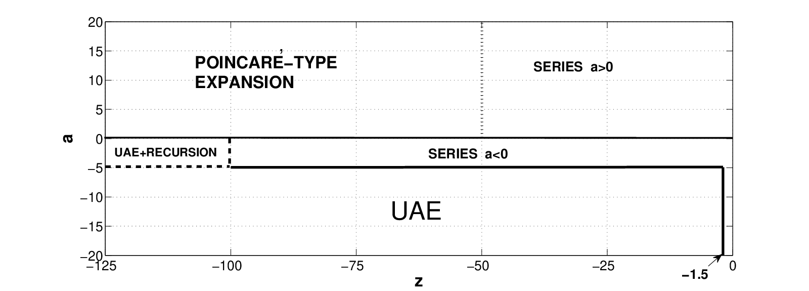
The resulting algorithm improves the range of computation of the algorithm presented in [18]. Thompson’s algorithm considers the computation of the lower incomplete gamma function for negative real values of the argument $z$ and half-integer values of the parameter $a$ using a function $S_{n}(z)$, $n$ integer and $z>0$, related to the lower incomplete gamma function by $\gamma(n+1/2,-z)=i(-1)^{n}e^{z}z^{n+1}S_{n}(z)$. The relation of the function $S_{n}(z)$ to the $\gamma^{*}(a,z)$ is then given by $S_{n}(z)=\Gamma(n+1/2)e^{-z}\gamma^{*}(n+1/2,-z)$. Precomputed values in Maple to initiate analytic continuation are used in Thompson’s algorithm which, in the implementation available in [18], seems to be restricted to $z$ values in the interval $[0,\,200]$. Our approach extends the range of computation to real values of the parameter $a$ and larger negative values of the argument $z$, and it does not depend on values precomputed in Maple.

The authors would thank the editors and reviewers for helpful suggestions and comments. The authors acknowledge financial support from Ministerio de Economía y Competitividad, project MTM2012-34787. NMT thanks CWI, Amsterdam, for scientific support.

References

- [1] D. H. Bailey and J. M. Borwein. Crandall’s computation of the incomplete Gamma function and the Hurwitz zeta function, with applications to Dirichlet L-series. Appl. Math. Comput., 268:462–477, 2015.
- [2] G.W. Collins. Fundamentals of Stellar Astrophysics. W H Freeman and Co, 1989.
- [3] A. Cuyt, V.B. Petersen, B. Verdonk, H. Waadeland, and W.B. Jones. Handbook of continued fractions for special functions. Springer, New York, 2008.
- [4] A.R. Didonato and A.H. Morris. Computation of the incomplete gamma function ratios and their inverse. ACM Trans. Math. Softw., 12:377–393, 1986.
- [5] W. Gautschi. A computational procedure for incomplete gamma functions. ACM Trans. Math. Softw., 5:466–481, 1979.
- [6] A. Gil, J. Segura, and N. M. Temme. Numerical methods for special functions. SIAM, Philadelphia, PA, 2007.
- [7] A. Gil, J. Segura, and N. M. Temme. Efficient and accurate algorithms for the computation and inversion of the incomplete gamma function ratios. SIAM J. Sci. Comput., 34(6):A2965–A2981, 2012.
- [8] V. Kowalenko. The modes of an ultra-cold strongly magnetized charged Bose gas. Eur. Phys. B, 1:161–168, 1998.
- [9] V. Kowalenko and N. E. Frankel. Asymptotics for the Kummer function of Bose plasmas. J. Math. Phys., 35(11):6178–6198, 1994.
- [10] K. Krishnamoorthy. Handbook of Statistical Distributions with Applications. Statistics: A Series of Textbooks and Monographs (Book 188). Chapman and Hall/CRC, 2006.
- [11] C. M. Linton. Lattice sums for the Helmholtz equation. SIAM Rev., 52(4):630–674, 2010.
- [12] A. Moroz. Quasi-periodic Green’s functions of the Helmholtz and Laplace equations. J. Phys. A: Math. Gen., 39:11247–11282, 2006.
- [13] A. B. Olde Daalhuis. Confluent hypergeometric functions. In NIST handbook of mathematical functions, pages 321–349. U.S. Dept. Commerce, Washington, DC, 2010.
- [14] F. W. J. Olver. Asymptotics and special functions. AKP Classics. A K Peters Ltd., Wellesley, MA, 1997. Reprint of the 1974 original [Academic Press, New York].
- [15] R. B. Paris. Incomplete gamma and related functions. In NIST handbook of mathematical functions, pages 175–192. U.S. Dept. Commerce, Washington, DC, 2010.
- [16] H. Takahasi and M. Mori. Double exponential formulas for numerical integration. Publ. Res. Inst. Math. Sci., 9:721–741, 1973/74.
- [17] N. M. Temme. Uniform asymptotics for the incomplete gamma functions starting from negative values of the parameters. Methods Appl. Anal., 3:335–344, 1996.
- [18] I. Thompson. Algorithm 926: Incomplete Gamma Functions with Negative Arguments. ACM Tran Math Soft, 39(2):Article 14, 2012.