Composite electronic orders induced by orbital Kondo effect

The simplest example of the orbital degrees of freedom is illustrated in Fig.1 where two electrons of up and down spins occupy either $p_{x}$ or $p_{y}$ orbital. In each orbital, two electrons form the spin singlet. The two orbital states are conveniently expressed in terms of pseudo-spin with $|+\rangle$ for the $p_{x}^{2}$ state and $|-\rangle$ for the $p_{y}^{2}$ state. With the tetragonal symmetry around the $z$-axis, the states $|\pm\rangle$ are degenerate.

Analogous situation occurs in actual $f$-electron systems with $f^{2}$ configuration under the crystalline electric field (CEF). However, the strong spin-orbit interaction makes the constituent $f$-electron states much more complicated. For example, the cubic CEF has doubly degenerate eigenstates labeled $\Gamma_{3}$, where the $f$-electron states have angular charge distributions such as $x^{2}-y^{2}$ and $3z^{2}-1$ with $x^{2}+y^{2}+z^{2}=1$. These charge distributions are regarded as orbitals. The operator describing the flipping of the orbital (or pseudo-spin) states $a,b$ is written as $X_{ab}=|a\rangle\langle b|$. Then the simplest local interaction between the $\Gamma_{3}$ states and conduction electrons is parameterized by the orbital exchange $J$, and is written as

$\displaystyle{\cal H}_{\rm ex}=\frac{J}{2}\sum_{ab}X_{ab}\sum_{\sigma}c^{\dagger}_{b\sigma}c_{a\sigma},$

(1)

where conduction electrons are characterized not only by the orbital $a,b$ but by the spin states $\sigma$. It is obvious that ${\cal H}_{\rm ex}$ is invariant under the point group operation. Precisely speaking, $\sigma$ describes one of a time reversal (Kramers) doublet, which also has an orbital component with spin-orbit interaction. For simplicity, however, we refer to $\sigma$ as ”real spin”. We use Latin characters such as $a,b$ for indices of pseudo-spins, and Greek characters such as $\alpha,\beta,\sigma,\rho$ for real spins.

The localized states with even number of $f$ electrons are called non-Kramers configurations. Pr³⁺ and U⁴⁺ with two $f$-electrons belong to such cases. Here the Kramers theorem about the time-reversal degeneracy does not apply, and the CEF ground state of a non-Kramers ion can either be a singlet, or a multiplet. Those systems such as PrAg₂In [22], PrMg₃ [23], PrPb₃[24] and PrTi₂Al₂₀[25] have doubly degenerate states as the CEF ground state. Since spatial distribution of wave functions in the doubly degenerate state are different from each other, an electric multipole such as quadrupole and hexadecapole should arise in the ordered phase. In addition, an imaginary coefficient in linear combination of wave functions brings about magnetic degree of freedom such as octupoles ($2^{3}$) and triakontadipoles ($2^{5}$).

There are two main sources as the origin of $J$: (i) Coulomb repulsion between $f$ and conduction electrons, and (ii) hybridization between them [14]. These sources are analogous to those for the spin exchange [26] where the Coulomb interaction favors the ferromagnetic interaction, while the hybridization favors the opposite sign [27]. Unfortunately, we are not aware of systematic study about the sign and magnitude of the orbital exchange $J$. We assume $J$ positive, which is necessary to have renormalization to strong coupling. If we have $J<0$, the higher-order effect drives the system to decoupled $f$ and conduction electrons [1]. Experimentally, there are many non-Kramers systems where $f$ electrons are localized well. It is likely that these systems have negative $J$. On the other hand, we expect $J>0$ for some U and Pr systems such as UBe₁₃ [17] and PrV₂Al₁₀ [18], which show behaviors analogous to those of canonical Kondo systems such as CeCu₂Si₂ and CeB₆ [9]. In general, $J$ tends to be positive and large as itinerant character of $f$ electrons becomes stronger.

In terms of the pseudo-spin operator $\hat{\bm{S}}$ for $f$ electrons, the orbital permutation in Eq.(1) is written as

$\displaystyle\sum_{ab\sigma}X_{ab}c^{\dagger}_{b\sigma}c_{a\sigma}=\sum_{ab\sigma}\left(\hat{\bm{S}}_{ab}\cdot c^{\dagger}_{b\sigma}\bm{\sigma}_{ba}c_{a\sigma}+\frac{1}{2}\delta_{ab}c^{\dagger}_{b\sigma}c_{a\sigma}\right),$

(2)

where $c_{a\sigma}$ is the annihilation operator of the conduction electron at the impurity site with orbital $a=1,2$ (or written as $\pm$ if convenient) and spin $\sigma=\uparrow,\downarrow$. The second term in the right-hand side (RHS) describes the potential scattering and will be neglected in the following. By adding the kinetic energy of conduction electrons we obtain the Hamiltonian of the two-channel Kondo impurity:

$\displaystyle{\cal H}_{\rm KI}$

$\displaystyle=\sum_{\bm{k}a\sigma}\varepsilon_{\bm{k}}c_{\bm{k}a\sigma}^{\dagger}c_{\bm{k}a\sigma}+J\hat{\bm{S}}\cdot(\hat{\bm{s}}_{\uparrow}+\hat{\bm{s}}_{\downarrow}),$

(3)

where $\hat{\bm{s}}_{\sigma}=\frac{1}{2}\sum_{ab}c^{\dagger}_{a\sigma}\bm{\sigma}_{ab}c_{b\sigma}$ is the pseudo-spin operator of conduction electrons with channel (real spin) components $\sigma$. The Hamiltonian (3) has the SU(2) symmetry in both spin and orbital degrees of freedom, which are written as SU(2)${}_{\rm S}\otimes$SU(2)_O.

Let us mention briefly other models of non-Kramers CEF states. If the CEF ground state is a singlet with small splitting $\Delta$ below a triplet, the spin Kondo effect occurs even for non-Kramers systems [28, 29, 30, 31]. In the simplest picture, each electron of $f^{2}$ configuration has the antiferromagnetic interaction $J_{2}$ with conduction electrons, and competes with $\Delta$. This situation is analogous to the two-impurity Kondo problem where the intersite interaction, often called the RKKY interaction, plays the role of $\Delta$. It is known that the two kinds of singlets, CEF and Kondo, crosses over in general as $J_{2}/\Delta$ increases from zero. If there is a higher symmetry, however, there appears a quantum critical point where the ground state shares the same feature as that of the two-channel Kondo model [32, 33]. It has been argued [9, 34] that a strange order in PrFe₄P₁₂ is a consequence of the competition between $J_{2}$ and $\Delta$. Recently another new model has been proposed [35] that takes the j-j coupling scheme to construct the $f^{2}$ CEF states. Depending on the strength of $J_{2}$ and the orbital exchange, either orbital or spin Kondo effect dominates over the other. Since we prefer a reasonable size of the review, the singlet CEF ground state will not further be discussed.

We prefer the term ”orbital Kondo effect” rather than the ”quadrupole Kondo effect” originally proposed [7], since the relevant multipole may be hexadecapole depending on the CEF states [36, 37]. Both spin and orbital types of Kondo effect bring about logarithmic temperature dependence $\ln T$ of the electrical resistivity $\rho(T)$ at temperatures higher than the characteristic temperature $T_{K}$, which is called Kondo temperature and gives the energy scale of the system. However, convincing examples of $\ln T$ behavior caused by the orbital Kondo effect are still lacking. For example the CEF doublet $\Gamma_{3}$ system PrTi₂Al₁₀ shows $\ln T$ behavior in $\rho(T)$ with maximum at $T\simeq 55$K as will be shown in Fig.11 later [25, 16]. The CEF level structure has been determined by neutron scattering as shown in Fig.2 [38].

Since the thermal population of first excited states ($n=2$) cannot be neglected for the temperature range $T>60$K, the origin of the $\ln T$ behavior may include magnetic exchange. More famous candidate of the orbital Kondo effect is UBe₁₃ where $\rho(T)$ increases with decreasing $T$, and saturates around $T\sim 40$ K[15], which is in sharp contrast with ordinary metals, and is often referred to as “non-Fermi liquid”. Superconductivity emerges below about 1 K from this non-Fermi liquid state [15] as will be shown in Fig.11 [17]. It is not trivial whether one can use the CEF picture in this material since the neutron scattering has probed only a broad feature [39].

On the other hand, Kondo effect is not seen in resistivity in such systems as PrAg₂In [22] and PrMg₃ [23], which neither show any symptom of electronic order at least down to 0.1 K. As a result, the $T$-coefficient of the specific heat becomes huge, reaching to several J/(mole$\cdot$K${}^{2})$. One of possible reasons for the absence of phase transition is splitting of the CEF doublet by crystalline disorder, which seems difficult to control in the Heusler structure [22, 23] . Another reason may be that the orbital exchange $J$ is negative, leading to ferro-coupling of $f$ and $c$ quadruples. Unfortunately, there has been no detailed study to evaluate $J$ for non-Kramers doublet systems taking realistic electronic structure. We concentrate from now on to the case $J>0$.

Let us briefly discuss the scaling theory and the non-trivial fixed point for the model ${\cal H}_{\rm KI}$. Following the elegant idea of Nozières and Blandin [8], we consider the hypothetical case where the number of screening channels is an arbitrary integer $n$. The dimensionless coupling constant $g\equiv J_{\rm eff}\rho_{c}$, with $\rho_{c}=1/(2D)$ being the density of states of conduction band, obeys the renormalization group (RG) (or scaling) equation [8]:

$\displaystyle\frac{dg}{dl}=-g^{2}+\frac{n}{2}g^{3}+O(ng^{4},n^{2}g^{5})$

(4)

with $\ell\equiv\ln(D_{\rm eff}/D)$. The simplest method to derive Eq.(4) will be the effective Hamiltonian formalism as detailed e.g. in Refs.\citenkuramoto00,kuramoto98. The scaling means roughly that the set $(J_{\rm eff},D_{\rm eff})$ gives the same low-energy physics as the combination of the bare quantities $(J,D)$. In other words, $J_{\rm eff}$ represents the $t$-matrix of a conduction electron with energy $D_{\rm eff}$[40].

The fixed point of the RG corresponds to zero of the RHS. Note that the third-order term has a factor $n$ because of participation of all screening channels. If we have a large value of $n$, which is actually unrealistic (but turns out useful), we may neglect the $O(g^{4})$ terms near the fixed point. We obtain $g=g_{c}$ at the fixed point as

$\displaystyle g_{c}=2/n,$

(5)

which is much smaller than unity with $n\gg 1$. Then the neglected $O(g^{4})$ terms are in fact smaller than the first two terms in the RHS.

Remarkably, this argument in Ref.\citennozieres80 remains qualitatively valid down to the realistic case of $n=2$. The essence of the validity comes from the physical phenomenon of “overscreening” that is common to all $n\ (>1)$. For example, if the local pseudo-spin makes a singlet with a conduction pseudo-spin with channel $\sigma$, another conduction channel $\bar{\sigma}$ still keeps the active orbital pseudo-spin. Hence the entropy of the system cannot go to zero. Figure 3 illustrates the effective coupling as a function of temperature $T$ which corresponds to $D_{\rm eff}$. Together with the renormalization to the non-trivial fixed point, we also show the case of the ordinary Kondo model including the renormalization at lowest order.

The non-trivial fixed point becomes unstable once the SU(2)${}_{\rm S}\otimes$SU(2)_O symmetry for spin and orbital spaces is broken by an external perturbation. For example, suppose that the orbital degeneracy of the local pseudo-spin is slightly broken by uniaxial pressure, which can be represented as a pseudo-Zeeman term $h_{z}\hat{S}_{z}$. Then the non-trivial ground state will change into the decoupled CEF singlet and the Fermi sea of conduction electrons with no remaining entropy. The effective coupling $g$ renormalizes to zero below the temperature corresponding to the splitting.

On the contrary, if the orbital exchange becomes larger for a channel than another, the effective coupling for that channel goes to infinity, and the other goes to zero. The ground state is a local Fermi liquid without residual entropy. Thus these important (relevant) perturbations are represented as [33]:

$\displaystyle V_{1}^{z}=h_{1}\hat{S}^{z},\quad V_{2}^{z}=h_{2}\hat{\bm{S}}\cdot(\hat{\bm{s}}_{\uparrow}-\hat{\bm{s}}_{\downarrow}),$

(6)

where $V_{1}^{z}$ has the pseudo magnetic field $h_{1}$ that breaks the non-Kramers degeneracy, and $V_{2}^{z}$ breaks the equivalence of two spin channels. Because of the SU(2)_S symmetry, we have also $x,y$ components for $V_{1},V_{2}$ as will be shown shortly. Note that $V_{1}^{z}$ involves only localized electrons, while $V_{2}^{z}$ is a composite object involving both local and conduction parts. Hence $V_{2}$ is more subtle and nontrivial.

We now focus on $V_{2}^{z}$ and regard $\hat{\bm{S}}\cdot(\hat{\bm{s}}_{\uparrow}-\hat{\bm{s}}_{\downarrow})$ as the $z$-component of a vector operator $\bm{\Psi}$. In general the $\mu$-component $\Psi^{\mu}$ with $\mu=x,y,z$ is given by

$\displaystyle\Psi^{\mu}=\frac{1}{2}\hat{\bm{S}}\cdot{\bm{\sigma}}_{ab}c_{a\sigma}^{\dagger}\sigma^{\mu}_{\sigma\rho}c_{b\rho}$

(7)

Here and in the rest of the present paper, we take the Einstein convention, if obvious, to omit summation symbols over repeated spin and orbital variables. It is convenient to introduce the combinations $\Psi^{\pm}=\Psi^{x}\pm i\Psi^{y}$ giving

$\displaystyle\Psi^{+}=\hat{\bm{S}}\cdot{\bm{\sigma}}_{ab}c^{\dagger}_{a\uparrow}c_{b\downarrow},\quad\Psi^{-}=\hat{\bm{S}}\cdot{\bm{\sigma}}_{ab}c^{\dagger}_{a\downarrow}c_{b\uparrow},$

(8)

which has flips of both real ($\uparrow,\downarrow$) and pseudo ($a,b$) spins.

Let us consider the case where the degenerate conduction bands have a particle-hole (PH) symmetry, which is realized if the degenerate conduction bands have flat density of states $\rho_{c}$ between the cut-offs $\pm D$, and the Fermi level is at the center of the band, i.e. $\mu=0$. With the PH symmetry, $\cal H_{\rm KI}$ in Eq.(3) commutes with corresponding generators. As an example we consider $P_{\sigma}$ for each spin (channel) $\sigma$ defined by

$\displaystyle P_{\sigma}c_{a\sigma}P_{\sigma}^{-1}=\epsilon_{ab}c^{\dagger}_{b\sigma},\quad P_{\sigma}c_{a\sigma}^{\dagger}P_{\sigma}^{-1}=\epsilon_{ab}c_{b\sigma},\quad$

(9)

where $\epsilon=i\sigma^{y}$ is the antisymmetric unit tensor. For $c_{a\rho}$ with $\rho\neq\sigma$, $P_{\sigma}$ behaves as the identity operator. It follows then

$\displaystyle P_{\sigma}c_{a\sigma}^{\dagger}{\bm{\sigma}}_{ab}c_{b\sigma}P_{\sigma}^{-1}=c_{a\sigma}^{\dagger}{\bm{\sigma}}_{ab}c_{b\sigma},$

(10)

without summation over $\sigma$. Namely the PH transformation conserves the pseudo-spin. Since the interaction in $\cal H_{\rm KI}$ depends only on the pseudo-spin, we obtain $[{\cal H}_{\rm KI},P_{\sigma}]=0$ under the PH symmetry.

By straightforward calculation we obtain

	$\displaystyle P_{\uparrow}\Psi^{+}P_{\uparrow}^{-1}$	$\displaystyle=\frac{1}{2}\hat{\bm{S}}\cdot(\epsilon{\bm{\sigma}})_{ab}\epsilon_{\sigma\rho}c_{a\sigma}c_{b\rho}\equiv\Phi\equiv\hat{\bm{S}}\cdot{\bm{t}},$		(11)
	$\displaystyle P_{\downarrow}\Psi^{+}P_{\downarrow}^{-1}$	$\displaystyle=\frac{1}{2}\hat{\bm{S}}\cdot({\bm{\sigma}\epsilon})_{ab}\epsilon_{\sigma\rho}c^{\dagger}_{a\sigma}c^{\dagger}_{b\rho}=\Phi^{\dagger}=\hat{\bm{S}}\cdot{\bm{t}}^{\dagger},$		(12)

where the quantities $\Phi$ and $\bm{t}$ are introduced. The operator $\bm{t}$ annihilates a pair of conduction electrons with channel singlet (Cs) and pseudo-spin triplet (St). Other combinations of $P_{\sigma}$ and $\Psi^{-}$ give either $\Phi$ or $\Phi^{\dagger}$. Here, following the literature [21, 46], we use the labels C and S indicating ‘channel’ and ‘spin’, and s and t indicating ‘singlet’ and ‘triplet’. This terminology is unfortunately confusing here since ‘spin’ means actually pseudo-spin (orbital) in our case, and ‘channel’ represents the real spin. With this caveat, we follow the conventional terms for easy comparison with the literature.

With $P_{\sigma}$ commuting with ${\cal H}_{\rm KI}$, Hermitian operators $\Psi^{\mu}\ (\mu=x,y,z)$ and $\Phi_{\rm R}=(\Phi+\Phi^{\dagger})/2,\Phi_{\rm I}=i^{-1}(\Phi-\Phi^{\dagger})/2$ have the same fluctuation spectrum. The quintet of operators thus represent a symmetry larger than the obvious one: SU(2)${}_{\rm S}\otimes$SU(2)_O. Namely, by incorporating the PH symmetry, the system acquires the SO(5) symmetry or, equivalently, the Sp(4) symplectic symmetry [33]. The operator $P_{\sigma}$ belongs to the set of Sp(4) generators. We shall return to this problem when we discuss the symmetry aspect of order parameters in later sections.

We now turn from the two-channel Kondo impurity to the lattice (2chKL) as a model of $f$-electron systems with non-Kramers doublets. The Hamiltonian is given by [42]

$\displaystyle{\cal H}_{\rm KL}=\sum_{\bm{k}a\sigma}\varepsilon_{\bm{k}}c_{\bm{k}a\sigma}^{\dagger}c_{\bm{k}a\sigma}+J\sum_{i\sigma}\hat{\bm{S}}_{i}\cdot\hat{\bm{s}}_{i\sigma},$

(13)

which is to be compared with ${\cal H}_{\rm KI}$.

In the lattice system, the residual entropy is removed by spontaneous breaking of the symmetry, namely by an electronic ordering. The simplest order has the mean-field described by $V_{1}^{z}$. Since this kind of order is connected continuously with a simple multipole order of localized electrons, characteristics peculiar to two channels may not appear. On the other hand, another order described by $V_{2}^{z}$ is more interesting since it breaks the time-reversal symmetry even with zero magnetic moment: $\langle\hat{\bm{s}}_{\uparrow}-\hat{\bm{s}}_{\downarrow}\rangle=0.$ In contrast with the ordinary Kondo lattice that can stay paramagnetic down to zero temperature, the 2chKL must have some kind of order because of the remaining entropy otherwise.

Let us first discuss symmetry breaking of channels, which usually corresponds to magnetic order of conduction electrons. We introduce the following operator dependent on imaginary times:

$\displaystyle O_{i}^{\rm ch}(\tau,\tau^{\prime})\equiv c_{ia\sigma}^{\dagger}(\tau)\sigma_{\sigma\rho}^{z}c_{ia\rho}(\tau^{\prime}).$

(14)

With a channel order, we obtain $\langle O_{i}^{\rm ch}(\tau,\tau)\rangle\neq 0$. However, the channel symmetry is broken even if the equal-time average is zero, provided $\langle O_{i}^{\rm ch}(\tau,\tau^{\prime})\rangle\neq 0$ for $\tau\neq\tau^{\prime}$. In particular, if the following quantity including the $\tau$-derivative:

$\displaystyle{\cal O}(\tau)\equiv\sum_{i}c_{ia\sigma}^{\dagger}(\tau)\sigma_{\sigma\rho}^{z}\dot{c}_{ia\rho}(\tau),$

(15)

has a finite average, the resulting order is an example of odd-frequency (OF) orders, which will be discussed in more detail later for superconductivity. Here we show that this order is equivalent to the homogeneous order of $\Psi^{z}$ defined by Eq.(7). Namely the commutator with ${\cal H}_{\rm KL}$ corresponding to the $\tau$-derivative gives

$\displaystyle{\cal O}=\sum_{\bm{k}}\varepsilon_{\bm{k}}c_{\bm{k}a\sigma}^{\dagger}\sigma_{\sigma\rho}^{z}c_{\bm{k}a\rho}+J\Psi^{z},$

(16)

where we have redefined

$\displaystyle\Psi^{z}\equiv\frac{1}{2}\sum_{i}\hat{\bm{S}}_{i}\cdot{\bm{\sigma}}_{ab}c_{ia\sigma}^{\dagger}\sigma^{z}_{\sigma\rho}c_{ib\rho},$

(17)

by including the site summation for the lattice system.

Let us consider how one can detect the composite order $\Psi^{z}$. Obviously the most interesting is the experimental detection, which is discussed later. In the numerical calculation for the 2chKL, the most powerful approach at present is the combination of the continuous-time quantum Monte Carlo (CT-QMC) [43] and the dynamical mean-field theory (DMFT) [44]. The basic idea is to use the CT-QMC to solve the impurity problem in the effective medium, which is determined self-consistently by the DMFT [13, 45]. Here we do not go into details of numerical methods, which have been reviewed in detail [43, 44]. It is possible to check whether $\Psi^{z}$ is finite or not at each temperature by direct evaluation. At the transition temperature, $\Psi^{z}$ begins to be finite and its fluctuation should diverge. However, it is difficult to compute the corresponding response function since $\Psi^{z}$ is a composite object.

Since the $\tau$-derivative form of $\cal O$ includes only conduction electrons, its response function may be derived without including localized electrons explicitly. Aiming at deriving the response function, we work with the two-particle Green function:

$\displaystyle\chi^{\rm ch}_{ij}(\tau_{1},\tau_{2},\tau_{3},\tau_{4})=\langle T_{\tau}O^{\rm ch}_{i}(\tau_{1},\tau_{2})O^{\rm ch}_{j}(\tau_{3},\tau_{4})\rangle,$

(18)

where $T_{\tau}$ is the time-ordering operator. We perform the Fourier transform to Matsubara frequencies $\varepsilon_{n}=(2n+1)\pi T$ as

	$\displaystyle\chi^{\rm ch}_{\bm{q}}(\mathrm{i}\varepsilon_{n},\mathrm{i}\varepsilon_{n^{\prime}})$	$\displaystyle=\frac{1}{N\beta^{2}}\sum_{ij}\int_{0}^{\beta}\hskip-5.69054pt\mathrm{d}\tau_{1}\cdots\mathrm{d}\tau_{4}\ \chi^{\rm ch}_{ij}(\tau_{1},\tau_{2},\tau_{3},\tau_{4})$
	$\displaystyle\times$	$\displaystyle\mathrm{e}^{-\mathrm{i}\bm{q}\cdot(\bm{R}_{i}-\bm{R}_{j})}\mathrm{e}^{\mathrm{i}\varepsilon_{n}(\tau_{2}-\tau_{1})}\mathrm{e}^{\mathrm{i}\varepsilon_{n^{\prime}}(\tau_{4}-\tau_{3})}.$		(19)

The response function of $\cal O$ is related to the derivative:

$\displaystyle\frac{\partial^{2}}{\partial\tau_{2}\partial\tau_{3}}\chi^{\rm ch}_{ij}(\tau_{1},\tau_{2},\tau_{3},\tau_{4}).$

(20)

The Fourier transform of Eq.(20) leads to factors $\mathrm{i}\varepsilon_{n}$ and $\mathrm{i}\varepsilon_{n^{\prime}}$. The $\tau$-derivatives in Eq.(20) also give rise to a delta-function part due to the time-ordering. In fact, one can prove the following relation [12]:

	$\displaystyle\hskip-28.45274pt\frac{1}{N}\int_{0}^{\beta}\langle{\cal O}(\tau){\cal O}^{\dagger}\rangle\mathrm{d}\tau=$
	$\displaystyle\hskip-28.45274pt-\frac{1}{\beta}\sum_{nn^{\prime}}\varepsilon_{n}\varepsilon_{n^{\prime}}\,\chi_{\bm{q}=0}^{\rm ch}(\mathrm{i}\varepsilon_{n},\mathrm{i}\varepsilon_{n^{\prime}})e^{\mathrm{i}\varepsilon_{n}0^{+}}e^{\mathrm{i}\varepsilon_{n^{\prime}}0^{+}}\hskip-2.84526pt+\hskip-2.84526pt\frac{2}{N}\langle{\cal H}\rangle,$		(21)

where convergence factors enter in frequency summations. The second term in the RHS comes from delta-functions associated with the time-ordering. Because of the second term, the sign of the first term is indefinite, even though the LHS is positive definite. This point is crucial in interpreting the numerical results for the OF susceptibilities.

At the transition temperature to the ordering of $\cal O$, the LHS and the first term in the RHS of Eq.(21) diverge. In the numerical calculation, the summation over Matsubara frequencies with convergence factors is very slow and awkward. Therefore alternative scheme has been proposed [21, 46]. Namely, one regards $\hat{\chi}_{nn^{\prime}}\equiv\chi_{\bm{q}=0}^{\rm ch}(\mathrm{i}\varepsilon_{n},\mathrm{i}\varepsilon_{n^{\prime}})$ as a matrix in the space of Matsubara frequencies. Then the divergence in Eq.(21) means that the maximum eigenvalue of $\hat{\chi}$ becomes infinity in the subspace of odd functions of $n$. Let us consider then what happens if one replaces $\varepsilon_{n}$ by another odd function $g_{n}$ in Eq.(21). As long as the eigen vector with the maximum eigenvalue has a finite overlap with both $\varepsilon_{n}$ and $g_{n}$, the divergence occurs at the same temperature. With this consideration one may choose $g_{n}=\tanh(\varepsilon_{n}/D)$ or simply $g_{n}={\rm sgn}(n)$. These choices lead to much faster convergence in the frequency summation.

Figure 4 shows the susceptibilities numerically derived at half-filling $n_{c}=2$ [12]. The staggered (AF) pseudo-spin susceptibility in panel (a) corresponds to the choice:

$\displaystyle O_{i}^{\rm orb}(\tau,\tau^{\prime})\equiv c_{ia\sigma}^{\dagger}(\tau)\sigma_{ab}^{z}c_{ib\sigma}(\tau^{\prime}),$

(22)

which actually corresponds to orbital degrees of freedom. The even-frequency (EF) part diverges at $T\sim 0.082$ with the unit $D=1$ for the half-width of the conduction bands with semi-elliptic density of states. The OF part remains finite for all temperatures. The homogeneous (F) channel susceptibility shown in panel (b) does not show any indication of divergence for the EF part. On the other hand, the OF part becomes negative as $T$ decreases, and then diverges from negative side at $T\sim 0.027$. The divergence indicates the onset of long-range order with $\Psi^{z}$. As we have remarked, the divergence is independent of the choice of $g_{n}$ although the magnitude of the susceptibility at higher temperature does depend on $g_{n}$.

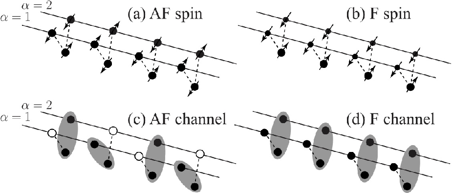
Figure 5 illustrates the ordering pattern with the conduction electron number $n_{\rm c}=1,2$ per site [12]. Physically the F channel order with $\Psi^{z}$ in (d) describes the breakdown of the spin symmetry; the orbital Kondo insulator appears involving down-spin $\alpha=2\ (\sigma=\downarrow)$ of conduction bands, while the up-spin ($\alpha=1$) conduction electrons make a Fermi liquid [11, 12]. The different spatial distributions of magnetic moments means the broken time-reversal, although there is no net magnetization. In this sense, the order parameter $\Psi^{z}$ represents a state with itinerant magnetic multipoles. If the non-Kramers degrees of freedom generates quadrupoles (hexadecapoles), $\Psi^{z}$ represents an itinerant octupole (triakontadipole) order. However, the orbital RKKY interaction makes the order (a) assigned as AF spin more stable than (d) with $n_{\rm c}=2$ [21]. In the non-Kramers system, (a) actually represents the AF orbital order. On the other hand, the AF-channel order (c), which is antiferromagnetism of real spins, is most stabilized at $n_{\rm c}=1$. The channel-symmetry breaking in (c) and (d) is a characteristic of the two-channel model, and cannot be explained by the RKKY interaction. Namely the Hamiltonian (13) includes only the interaction between pseudo-spins rather than channels.

Surprisingly, the F-channel ($\Psi^{z}$) order is converted to a composite superconductivity by a unitary transformation. This is a consequence of the hidden SO(5) symmetry as will be discussed in greater detail later. The overall phase diagram of the 2chKL will be shown later in Fig. 8.

Now we consider the single-particle spectrum for the F-channel order, which leads us to the simple effective Hamiltonian at low energies. We define the spectrum for the component $a,\sigma$ by

$\displaystyle A_{a\sigma}(\bm{k},\omega)=-\frac{1}{\pi}\mathrm{Im}\,G_{a\sigma}(\bm{k},\omega+\mathrm{i}\eta),$

(23)

where $\eta=+0$. The single-particle Green function is given by

$\displaystyle G_{a\sigma}(\bm{k},z)^{-1}=z-\varepsilon_{\bm{k}}-\Sigma_{a\sigma}(z),$

(24)

where $z$ is a complex energy and $\Sigma_{a\sigma}(z)$ is the self energy. In the DMFT, the wave-vector dependence enters into the single-particle Green function only through $\varepsilon_{\bm{k}}$.

The spectrum in the paramagnetic state has a broad feature (not shown), which is consistent with the incoherent metallic state [42]. The peak energy at each momentum is almost the same as the non-interacting one[13]. This non-Fermi liquid behavior originates from interaction of localized spins with overscreening degenerate channels. In particular the Kondo singlet state cannot be formed.

Figure 6 shows the numerical result [12, 13] in the ordered phase.

The parameter $\kappa$ is introduced by $\varepsilon_{\bm{k}}=-D\cos\kappa$ so that the spectrum is visualized as if in a one-dimensional system. The spectrum for channel (real spin) $\alpha=2$ is clearly characterized by a hybridization with localized levels precisely at the Fermi level. On the other hand, the spectrum for $\alpha=1$ shows a Fermi liquid behavior with sharp Fermi surface. The broadening becomes substantial away from the Fermi level. Near the Fermi level, the Green function for both channels are parameterized as

	$\displaystyle G_{a\sigma}(\bm{k},z)$	$\displaystyle\sim\frac{a_{\sigma}}{z-a_{\sigma}\varepsilon_{\bm{k}}-a_{\sigma}{V_{\sigma}}^{2}/z},$		(25)
	$\displaystyle\Sigma_{a\sigma}(z)$	$\displaystyle=\frac{{V_{\sigma}}^{2}}{z}+b_{\sigma}z+O\left(z^{2}\right),$		(26)

where the renormalization factor is given by $a_{\sigma}=(1-b_{\sigma})^{-1}$. For $\alpha=1\ (\sigma=\uparrow)$, numerical analysis of the self-energy [13] gives $a_{\uparrow}\simeq 0.51$ and $V_{\uparrow}\simeq 0.00$ at $T=0.005$. This means that the conduction electrons with spin up shows the Fermi-liquid behavior, and hybridization is absent. For $\alpha=2\ (\sigma=\downarrow)$, on the other hand, the values obtained are $a_{\downarrow}\simeq 0.43$, $V_{\downarrow}\simeq 0.33$. This indicates the behavior of the Kondo insulator with effective hybridization $V_{\downarrow}$. Thus, the spectrum displays the admixture of the Fermi liquid and Kondo insulator. From Fig.6 it is apparent that hybridization gap in down spins causes lower kinetic energy than up spins. Then we recognize that both constituents of the operator $\cal O$ in Eq.(16) have non-zero average in the ordered phase.

Away from half filling, there emerges a doped Kondo insulator for $\sigma=\downarrow$ which behaves as heavy Fermi liquid at sufficiently low temperature. The ordered phase in the doped case then consists of two different Fermi liquids dependent on channels.

The effective hybridization picture, which corresponds to the strong-coupling limit ($J\rightarrow\infty$), has already been used for the standard Kondo lattice [2, 3]. In the present case, the channel-symmetry breaking is essential to realize the effective hybridization. Namely, in the paramagnetic state, we do not see any indication of hybridization in contrast to the ordinary Kondo lattice.

We have shown for the impurity system that leading fluctuations consist of a three-component vector $\bm{\Psi}$, Eq.(7), and pairing fluctuations $\Phi,\Phi^{\dagger}$, Eq.(12). With the PH symmetry in half-filled conduction bands, these five fluctuations have exactly the same spectrum. The underlying SO(5) symmetry remains effective also for the lattice system described by ${\cal H}_{\rm KL}$. In particular a symmetry-broken ground state has the same energy with other four symmetry-broken states. Moreover, the excitation spectra are also common to these ordered phases as will be demonstrated in section 4.4.

Let us proceed to off-diagonal orders with particular attention to the symmetry aspect. We assume the bipartite lattice with A, B sublattices, and introduce the site-dependent PH transformation:

$\displaystyle P_{\downarrow}c_{ia\downarrow}P_{\downarrow}^{-1}=\pm\epsilon_{ab}c_{ib\downarrow}^{\dagger}$

(27)

where the sign factor is +1 for A and -1 for B sublattices. Equivalently one may use $\exp({\rm i}\bm{Q}\cdot\bm{R}_{i})=\pm 1$ with $\bm{Q}$ corresponding to the staggered order. Because of the phase factor, the hopping term between the nearest-neighbor sites remains the same under the PH transformation. The invariance can be illustrated by the hopping of spin-down electrons:

$\displaystyle tc_{{\rm A}a}^{\dagger}c_{{\rm B}a}$

$\displaystyle\rightarrow-tc_{{\rm A}b}c_{{\rm B}b}^{\dagger}=tc_{{\rm B}b}^{\dagger}c_{{\rm A}b},$

(28)

where the site indices are replaced by the sublattice indices A and B, and the spin indices are omitted. The up-spin electrons are not affected by $P_{\downarrow}$.

The PH transformation $P_{\downarrow}$ for $\Psi^{+}$ gives

	$\displaystyle P_{\downarrow}\Psi^{+}P_{\downarrow}^{-1}$	$\displaystyle=\frac{1}{2}\sum_{i}e^{{\rm i}\bm{Q}\cdot\bm{R}_{i}}\hat{\bm{S}}_{i}\cdot\left({\bm{\sigma}}\epsilon\right)_{ab}\epsilon_{\sigma\rho}c^{\dagger}_{ia\sigma}c^{\dagger}_{b\rho}$
		$\displaystyle\equiv\Phi(\bm{Q})^{\dagger},$		(29)

which is to be compared with Eq.(12) for the impurity system. Here $\Phi(\bm{Q})^{\dagger}$ represents a staggered and composite superconducting order. In the same way, we can show

$\displaystyle P_{\downarrow}\Psi^{-}P_{\downarrow}^{-1}=\Phi(\bm{Q}),\quad P_{\downarrow}\Psi^{z}P_{\downarrow}^{-1}=\Psi^{z}.$

(30)

On the other hand, explicit calculation shows

$\displaystyle P_{\downarrow}\Phi(\bm{Q})P_{\downarrow}^{-1}=-\Psi^{-},$

(31)

which also follows immediately from the definition given by Eq.(27).

It is instructive to take the strong coupling limit for visualizing the nature of composite order $\Phi$. Suppose we have a doublet of either (i) pseudo-spin or (ii) channel at each site. In each case, we can combine the doublets of two sites to make a singlet. For a finite-sized Hamiltonian, however, we cannot have the symmetry-broken eigenstate. Hence we shall deal with local eigenstates of the Hermitian operator $\Phi_{\rm R}=(\Phi+\Phi^{\dagger})/2$.

Let us begin with the case (i) for a single site. We start from the state $|0\rangle\otimes|\pm\rangle\equiv|0\pm\rangle$ where $|0\rangle$ is a vacuum of conduction electrons, and $|\pm\rangle$ is the $f$-state doublet. Then we obtain

	$\displaystyle\Phi^{\dagger}|0\rangle\otimes|+\rangle$	$\displaystyle=2|{\rm CsSt}_{1}\rangle\otimes|-\rangle+|{\rm CsSt}_{0}\rangle\otimes|+\rangle$
		$\displaystyle\equiv\sqrt{5}|2+\rangle,$		(32)

where the pseudo-spin triplets of two electrons with $z$-components 1,0 are given by

	$\displaystyle|{\rm CsSt}_{1}\rangle$	$\displaystyle=c_{+\uparrow}^{\dagger}c_{+\downarrow}^{\dagger}|0\rangle,$		(33)
	$\displaystyle|{\rm CsSt}_{0}\rangle$	$\displaystyle=\frac{1}{2}\sigma^{x}_{ab}\epsilon_{\sigma\rho}c_{a\sigma}^{\dagger}c_{b\rho}^{\dagger}|0\rangle,$		(34)

Figure 7 illustrates these states.

On the other hand, starting from $|\tilde{0}\rangle\otimes|+\rangle\equiv|\tilde{0}+\rangle$ where $|\tilde{0}\rangle$ is the fully occupied state with $n_{c}=4$, we obtain the same state by

$\displaystyle\Phi|\tilde{0}+\rangle=\sqrt{5}|2+\rangle=\Phi^{\dagger}|0+\rangle.$

(35)

Hence $\Phi_{\rm R}=(\Phi+\Phi^{\dagger})/2$ is represented by a $3\times 3$ matrix with the basis set $|0+\rangle,|2+\rangle$ and $|\tilde{0}+\rangle$. We can repeat the same analysis starting from $|0-\rangle$. The eigenvalues $x_{\mu}$ and corresponding eigenvectors $\phi_{\mu}(a)$ with $\mu=0,\pm$ and $a=\pm$ are derived as

	$\displaystyle x_{0}$	$\displaystyle=0:\quad\phi_{0}(a)=\left(|0a\rangle+|\tilde{0}a\rangle\right)/{\sqrt{2}},$		(36)
	$\displaystyle x_{\pm}$	$\displaystyle=\sqrt{10}:\quad\phi_{\pm}(a)=|2+\rangle/\sqrt{2}\pm\left(|0a\rangle+|\tilde{0}a\rangle\right)/2.$		(37)

We now consider two-site system and combine the states $\phi_{i\mu}(a)$ with $\mu=\pm$ for the sites $i=1,2$ to make a pseudo-spin singlet. We obtain both homogeneous and staggered states, the latter of which is given by

$\displaystyle\phi_{12}(\bm{Q})\equiv\frac{1}{2}\epsilon_{ab}\epsilon_{\mu\nu}\phi_{1\mu}(a)\phi_{2\nu}(b),$

(38)

with the eigenvalue $2\sqrt{10}$ for $\Phi_{1\rm R}-\Phi_{2\rm R}$, while zero eigenvalue for $\Phi_{1\rm R}+\Phi_{2\rm R}$. Furthermore the state is the singlet of both channel and pseudo-spin.

In the case (ii) we only briefly sketch the construction. Let us start from the state $\chi_{\sigma}$ described by

$\displaystyle\chi_{\sigma}=\frac{1}{\sqrt{2}}\epsilon_{ab}c_{a\sigma}^{\dagger}|b\rangle,$

(39)

where $|b\rangle$ with $b=\pm$ represents the doublet of local $f$-electron states. The state $\chi_{\sigma}$ is channel ($\sigma$) doublet (Cd) and pseudo-spin singlet (Ss). Application of $\Phi^{\dagger}$ to $\chi_{\sigma}$ creates another doublet with $n_{c}=3$, and further application of $\Phi$ brings back to $\chi_{\sigma}$. Thus $\Phi_{\rm R}$ is represented by a $2\times 2$ matrix proportional to $\sigma^{x}$. Proceeding in a similar manner as in the case (i), we obtain a staggered CsSs state where $\Phi_{1\rm R}-\Phi_{2\rm R}$ is finite. Note that inclusion of transfer of electrons between the sites 1,2 mixes the singlet states of (i) and (ii).

In the half-filled case $n_{c}=2$, the wave function of the symmetry-broken macroscopic state consists of linear combination of the products of local states obtained above. Without the transfer term, the expectation value of the Hamiltonian is the same in the staggered and homogeneous $\Phi$ states. With the transfer term, however, only the staggered state is degenerate with the $\Psi^{\mu}$ order which gains the kinetic energy by homogeneous symmetry breaking.

As in the case of diagonal orders, the composite off-diagonal order can be regarded as an odd-frequency (OF) order of conduction electrons [20, 19]. This identification is very useful in deriving the phase transition numerically from the disordered side. Namely, one can search for divergence of the OF response function including only conduction electrons, which is much simpler than treating the composite operator directly.

We explain more details of the OF order taking a pairing function with symbolic notation:

$\displaystyle F_{\mu\nu}(\tau)\equiv-\langle T_{\tau}c_{\mu}(\tau)c_{\nu}\rangle=\psi_{0}+\tau\psi_{\rm odd}+\tau^{2}\psi_{2}+\cdots,$

(40)

where $\mu,\nu$ are quantum numbers such as spin, orbital or momentum. If $\psi_{0}=\langle c_{\mu}c_{\nu}\rangle\neq 0$, we have an ordinary pairing. On the other hand, if we have $\psi_{0}=0$ but $\psi_{\rm odd}=\langle\dot{c}_{\mu}c_{\nu}\rangle\neq 0$, there is no ordinary pairing, but the gauge symmetry is surely broken. Such state is called the OF pairing in the literature [48, 50, 19]. The anticommutation property of fermions requires:

$\displaystyle F_{\mu\nu}(\tau)=-F_{\nu\mu}(-\tau).$

(41)

Without exchange of the indices $\mu,\nu$, however, the $\tau$-dependence is in general neither even nor odd. For example, it is possible to have $\psi_{\rm odd}\psi_{2}\neq 0$ in Eq.(40). We shall present such an example later in Eq.(75). The crucial point of the exotic pairing is not so much the temporal parity but that $F_{\mu\nu}(\tau)\neq 0$ with $\tau\neq 0$, even though $\psi_{0}=0$. This is evident if one considers systems without inversion symmetry where the spatial parity is not conserved. Then the temporal parity is mixed even for simple pairings [51].

The fermionic symmetry is made explicit in the frequency space as

	$\displaystyle F_{\mu\nu}(z)$	$\displaystyle=\sum_{mn}\frac{\rho_{n}+\rho_{m}}{z-E_{n}+E_{m}}(c_{\mu})_{mn}(c_{\nu})_{nm}$
		$\displaystyle=-F_{\nu\mu}(-z),$		(42)
	$\displaystyle\bar{F}_{\nu\mu}(z)$	$\displaystyle\equiv\sum_{mn}\frac{\rho_{n}+\rho_{m}}{z-E_{n}+E_{m}}(c_{\nu}^{\dagger})_{mn}(c_{\mu}^{\dagger})_{nm}$
		$\displaystyle=F_{\mu\nu}(z^{*})^{*}$		(43)

where $\rho_{n}$ is the statistical weight of each grand-canonical state $n$ which is superposition of different electron numbers. Hence the corresponding energy $E_{n}$ includes the chemical potential, and $z$ denotes complex frequency appearing through analytic continuation from Matsubara frequencies $i\varepsilon_{n}$ [3]. Precisely speaking, the gauge-broken states characterized by $\rho_{n}$ are meaningful only in the thermodynamic limit with the quasi-average [52].

In analogy to $\Psi^{z}$, we regard $\Phi(\bm{Q})$ as a part of the corresponding odd-frequency order parameter. Namely we define

	$\displaystyle{\cal O}(\bm{Q})$	$\displaystyle=\epsilon_{\sigma\rho}\epsilon_{ab}\sum_{i}\exp({\rm i}\bm{Q}\cdot\bm{R}_{i})c_{ia\sigma}\dot{c}_{ib\rho}$
		$\displaystyle\equiv{\cal O}_{1}(\bm{Q})+{\cal O}_{2}(\bm{Q}),$		(44)

where the decomposition is analogous to ${\cal O}^{z}$ in Eq.(15), as given by

	$\displaystyle{\cal O}_{1}(\bm{Q})$	$\displaystyle={\epsilon_{ab}}{\epsilon_{\sigma\rho}}\sum_{\bm{k}}\varepsilon_{\bm{k}}c_{\bm{k}a\sigma}c_{-\bm{k}-\bm{Q}\,b\rho},$
	$\displaystyle{\cal O}_{2}(\bm{Q})$	$\displaystyle=J\Phi(\bm{Q}).$		(45)

Note that the staggered nature of ${\cal O}_{1}(\bm{Q})$ is analogous to the $\eta$-pairing [53]. The differences however are first the presence of orbital degeneracy, and secondly the factor $\varepsilon_{\bm{k}}$ in the $\bm{k}$-summation. The latter implies the finite pairing amplitude at different sites, since $\varepsilon_{\bm{k}}$ corresponds to the transfer $t_{ij}$ between sites $i,j$ in the site representation. As in the case of Eq.(16), both ${\cal O}_{1}(\bm{Q}),{\cal O}_{2}(\bm{Q})$ acquire finite value in the ordered phase. Hence the on-site composite pairing mixes with an off-site EF pairing [75].

Let us introduce the following operators dependent on imaginary times to describe possible pairings:

	$\displaystyle\displaystyle O_{i}^{\rm CsSs}(\tau,\tau^{\prime})$	$\displaystyle=\epsilon_{ab}\epsilon_{\sigma\rho}c_{ia\sigma}(\tau)c_{ib\rho}(\tau^{\prime}),$		(46)
	$\displaystyle\displaystyle O_{i}^{\rm CtSs}(\tau,\tau^{\prime})$	$\displaystyle=\epsilon_{ab}c_{ia\sigma}(\tau)c_{ib\sigma}(\tau^{\prime}),$		(47)
	$\displaystyle\displaystyle O_{i}^{\rm CsSt}(\tau,\tau^{\prime})$	$\displaystyle=\epsilon_{\sigma\rho}c_{ia\sigma}(\tau)c_{ia\rho}(\tau^{\prime}),$		(48)
	$\displaystyle\displaystyle O_{i}^{\rm CtSt}(\tau,\tau^{\prime})$	$\displaystyle=c_{ia\sigma}(\tau)c_{ia\sigma}(\tau^{\prime}).$		(49)

where the triplet (t) has picked up the simplest component ($d_{y}$) out of the general combinations specified by the $d$-vector [3].

Note that $O_{i}^{\rm CsSs}(\tau,\tau)=O_{i}^{\rm CtSt}(\tau,\tau)=0$ due to the Pauli principle. In order to calculate susceptibilities, we introduce the two-particle Green function by

$$\chi^{\rm CS}_{ij}(\tau_{1},\tau_{2},\tau_{3},\tau_{4})=\langle T_{\tau}O^{\rm CS}_{i}(-\tau_{2},-\tau_{1})^{\dagger}O^{\rm CS}_{j}(\tau_{3},\tau_{4})\rangle$$

where $\rm CS$ represents one of the labels in Eqs. (46–49). Using this quantity and the $\tau$-derivatives as in Eq.(20), we define the even-frequency (EF) and OF pairing susceptibilities $\chi_{\bm{q}}^{\rm CS}$ with $\rm CS\rightarrow\rm EF,OF$ by

	$\displaystyle\chi_{\bm{q}}^{\rm EF}$	$\displaystyle=\frac{1}{\beta}\sum_{nn^{\prime}}\chi^{\rm EF}_{\bm{q}}(\mathrm{i}\varepsilon_{n},\mathrm{i}\varepsilon_{n^{\prime}}),$		(50)
	$\displaystyle\chi_{\bm{q}}^{\rm OF}$	$\displaystyle=\frac{1}{\beta}\sum_{nn^{\prime}}g_{n}g_{n^{\prime}}\chi^{\rm OF}_{\bm{q}}(\mathrm{i}\varepsilon_{n},\mathrm{i}\varepsilon_{n^{\prime}}),$		(51)

where $\rm EF$ corresponds to CsSt or CtSs, while $\rm OF$ to CsSs or CtSt.

For the OF pairing, a form factor $g_{n}={\rm sgn}\,\varepsilon_{n}$ makes the calculation much easier than using $\varepsilon_{n}$ [21, 46, 54] The EF susceptibility must be positive definite. On the other hand, the OF susceptibility given by Eq. (51) has the additional contribution corresponding to the second term in the RHS of Eq.(21). Then the sign of the OF susceptibility is indefinite. It seems that the additional contribution was overlooked in Refs.\citenjarrell97,cox98, where the sign change of the response function was interpreted as a first-order transition. The lowest temperature in the previous calculation is apparently still higher than the instability toward an OF order.

Figure 8(a) shows the temperature dependence of $\chi^{\rm CS}_{\bm{q}}$ at $J=0.8$ and $n_{\rm c}=1.5$ [13]. Here the two ordering vectors $\bm{q}=\bm{0}$ and $\bm{q}=\bm{Q}$ are considered, which are called ferro (F) and antiferro (AF), respectively. Among the eight susceptibilities, only the one with AF-CsSs diverges at $T_{\rm sc}\simeq 0.024$ signaling the onset of the staggered OF superconductivity. Note that the divergence occurs from the negative side as temperature is decreased. Since the normal state of the 2chKL is a non-Fermi liquid as seen in electrical resistivity [42] and thermodynamic quantities [13], the present system becomes superconducting directly from the non-Fermi liquid. Figure 9 shows a model calculation[55] of the resistivity, which is consistent with the original result [42] except for detection of superconductivity.

Together with the diagonal orders that have been obtained in a similar manner [13], the phase diagram of the 2chKL is completed as shown in Fig. 8(b). Here the diagonal orders are characterized by the vector operators

		$\displaystyle\hat{\bm{S}}(\bm{q})=\sum_{i}\hat{\bm{S}}_{i}\mathrm{e}^{-\mathrm{i}\bm{q}\cdot\bm{R}_{i}},$		(52)
		$\displaystyle\bm{\tau}_{\rm c}(\bm{q})=\sum_{i}\bm{\sigma}_{\sigma\rho}c^{\dagger}_{ia\sigma}c_{ia\rho}\mathrm{e}^{-\mathrm{i}\bm{q}\cdot\bm{R}_{i}},$		(53)
		$\displaystyle\bm{\Psi}(\bm{q})=\frac{1}{2}\sum_{i}(\hat{\bm{S}}_{i}\cdot\bm{\sigma}_{ab})\bm{\sigma}_{\sigma\rho}c^{\dagger}_{ia\sigma}c_{ib\rho}\mathrm{e}^{-\mathrm{i}\bm{q}\cdot\bm{R}_{i}},$		(54)

which describe localized pseudo-spin or orbital ($\hat{\bm{S}}$), itinerant real-spin or channel ($\bm{\tau}_{\rm c}$), and composite ($\bm{\Psi}$) orders, respectively. The instability toward superconductivity is found in almost all range of the filling unlike the diagonal orders. This feature seems characteristic of off-diagonal orders as also seen in the attractive Hubbard model [57].

The inset of Fig. 8(b) shows the transition temperature at $n_{\rm c}=1.5$ as a function of $J$, where only the superconductivity is found at $T\geq 0.001$. Note that the transition temperature for $J\lesssim 0.8$ scales with the Kondo temperature $T_{\rm K}\propto\exp[-1/\rho(\mu)J]$ derived in the weak coupling limit. The value $J=0.8$ was chosen simply for easier calculation, but it turns out that the value is still in the regime following the weak coupling behavior.

In closing this subsection we mention the result for a related model called the two-channel, or SU(2)$\times$SU(2), Anderson lattice [14, 46]. It has been reported that a homogeneous OF pairing with the CtSt symmetry is realized only in the presence of charge fluctuation of $f$-electrons [46]. Here the calculation uses the extension of the resolvent method called the NCA [2, 3]. It is highly desirable to check the result with more accurate numerical methods such as the CT-QMC.

At half filling, the transition temperatures for the AF-CsSs $[\bm{\Phi}(\bm{Q})]$ and F channel $[\bm{\Psi}(\bm{0})]$ orders are the same within the numerical accuracy as seen in Fig. 8(b). This degeneracy is a consequence of the SO(5) symmetry. Let us explore further consequence of the symmetry in excitation spectra. For this purpose we take the total single-particle spectrum defined by

$\displaystyle A(\bm{k},\omega)\equiv-\frac{1}{\pi}{\rm Im}\ {\rm Tr}\ G(\bm{k},\omega+\mathrm{i}\eta),$

(55)

where the Green function is regarded as a $4\times 4$ matrix, and Tr means summation over pseudo-spin ($a$) and channel ($\sigma$) indices.

Figure 10 shows the numerical result in the superconducting phase [55].

Surprisingly, the spectrum looks exactly like the spin sum in the $\Psi^{z}$ ordered phase shown in Fig.6, even though the nature of the superconducting order is very different from the diagonal composite order. To understand the identical spectrum, we work with the Nambu representation of the Green function with eight components $\nu=1,\ldots,8$:

$\displaystyle\psi_{\nu}(\bm{k})=(c_{a\sigma}(\bm{k}),h_{a\sigma}(\bm{k})),$

(56)

where $c_{a\sigma}$ corresponds to $\nu\leq 4$, while $h_{a\sigma}$ corresponds to $\nu\geq 5$. The latter can be identified as hole annihilation operators defined by

$\displaystyle h_{a\sigma}(\bm{k})={\epsilon_{ab}}{\epsilon_{\sigma\rho}}c_{b\rho}(-\bm{k}+\bm{Q})^{\dagger}.$

(57)

We have seen that the PH transformation $P_{\downarrow}$ changes the operator $\Psi^{+}$ to $\Phi^{\dagger}$, or equivalently $\Psi^{-}$ to $\Phi$. Namely, starting from an ordered state $|\psi^{-}\rangle$ with $\langle\psi^{-}|\Psi^{-}|\psi^{-}\rangle\neq 0$, we obtain

$\displaystyle\langle\phi_{s}|\Phi(\bm{Q})|\phi_{s}\rangle\neq 0,$

(58)

where $\phi_{s}=P_{\downarrow}\psi^{-}$ has the same energy as $\psi^{-}$. If a physical quantity is invariant under $P_{\downarrow}$, the expectation value of the quantity is common to the ordered states $\psi_{-}$ and $\phi_{s}$. We now show that the quantity

$\displaystyle\psi_{\nu}(\tau)\psi_{\nu}^{\dagger}$

(59)

summed over eight components remains invariant under $P_{\downarrow}$. More generally, any transformation $S$ within the SO(5) symmetry gives

$\displaystyle S\psi_{\nu}S^{-1}=\psi_{\mu}U_{\mu\nu},$

(60)

with $\{U_{\mu\nu}\}$ being a unitary matrix. Then summation over the components $\nu$ gives

$\displaystyle S\psi_{\nu}(\tau)\psi_{\nu}^{\dagger}S^{-1}=\psi_{\nu}(\tau)\psi_{\nu}^{\dagger}.$

(61)

Taking $S=P_{\downarrow}$, in particular, we obtain

$\displaystyle\langle\phi_{s}|S\psi_{\nu}(\tau)\psi_{\nu}^{\dagger}S^{-1}|\phi_{s}\rangle=\langle\psi_{-}|\psi_{\nu}(\tau)\psi_{\nu}^{\dagger}|\psi_{-}\rangle,$

(62)

Hence the Fourier transform Tr $G$ is also common to diagonal and off-diagonal orders. Repeating the same argument for each excited state, we conclude that the spectrum at finite temperature is also identical between $\Phi$ and $\Psi^{z}$ orders.

References

- [1] J. Kondo: Resistance Minimum in Dilute Magnetic Alloys, Prog. Theor. Phys. 32 (1964) 34.
- [2] A. C. Hewson: The Kondo Problem to Heavy Fermions (Cambridge University Press, 1993).
- [3] Y. Kuramoto and Y. Kitaoka: Dynamics of Heavy Electrons (Oxford University Press, 2000).
- [4] D. Goldhaber-Gordon et al.: Kondo effect in a single-electron transistor, Nature 391 (1998) 156.
- [5] S. K. Goh et al.: Anomalous upper critical field in CeCoIn5/YbCoIn5 superlattices with a Rashba-type heavy Fermion interface, Phys. Rev. Lett. 109 (2012) 157006.
- [6] K. Hattori, K. Itakura, S. Ozaki, and S. Yasui: QCD Kondo effect: Quark matter with heavy-flavor impurities, Phys. Rev. D 92 (2015) 065003; S. Ozaki, K. Itakura and Y. Kuramoto: Magnetically Induced QCD Kondo Effect, arXiv:1509.06966v1.
- [7] D. L. Cox: Quadrupolar Kondo effect in uranium heavy-electron materials?, Phys. Rev. Lett. 59 (1987) 1240.
- [8] Ph. Nozières and A. Blandin: Kondo effect in real metals, J. Physique 41 (1980) 193.
- [9] Y. Kuramoto, H. Kusunose and A. Kiss: Multipole Orders and Fluctuations in Strongly Correlated Electron Systems, J. Phys. Soc. Jpn. 78 (2009) 072001.
- [10] P. Santini et al.: Multipolar interactions in f-electron systems: The paradigm of actinide dioxides, Rev. Mod. Phys. 81 (2009) 807.
- [11] R. Nourafkan and N. Nafari: Kondo lattice model at half-filling, J. Phys. Condens. Matter 20 (2008) 255231.
- [12] S. Hoshino, J. Otsuki and Y. Kuramoto: Diagonal composite order in a two-channel Kondo lattice, Phys. Rev. Lett. 107 (2011) 247202.
- [13] S. Hoshino, J. Otsuki and Y. Kuramoto: Resolution of Entropy by Ordering in Two-Channel Kondo Lattice, J. Phys. Soc. Jpn. 82 (2013) 044707.
- [14] D. L. Cox and A. Zawadowski: Exotic Kondo effects in metals: magnetic ions in a crystalline electric field and tunnelling centres, Adv. Phys. 47 (1998) 599.
- [15] H. R. Ott, H. Rudigier, Z. Fisk and J. I. Smith: UBe13: An Unconventional Actinide Superconductor, Phys. Rev. Lett. 50 (1983) 1595.
- [16] K. Matsubayashi et al.: Pressure-induced heavy fermion superconductivity in the nonmagnetic quadrupolar system PrTi2Al20, Phys. Rev. Lett. 109 (2012) 187004.
- [17] Y. Shimizu et al.: Non-Fermi-liquid nature and exotic thermoelectric power in the heavy-fermion superconductor UBe13, Phys. Rev. B 92 (2015) 241101(R).
- [18] M. Tsujimoto et al: Heavy-fermion superconductivity in the quadrupole ordered state of PrV2 Al20, Phys. Rev. Lett. 113 (2014) 267001.
- [19] V. J. Emery and S. Kivelson: Mapping of the two-channel Kondo problem to a resonant-level model, Phys. Rev. B 46 (1992) 10812.
- [20] E. Abrahams, A. Balatsky, J. R. Schrieffer and P. B. Allen: Interactions for odd--gap singlet superconductors, Phys. Rev. B 47 (1993) 513.
- [21] M. Jarrell, H. Pang and D. L. Cox: Phase Diagram of the Two-Channel Kondo Lattice , Phys. Rev. Lett. 78 (1997) 1996.
- [22] A. Yatskar, W. P. Beyermann, R. Movshovich, and P. C. Canfield: Possible Correlated-Electron Behavior from Quadrupolar Fluctuations in PrInAg2, Phys. Rev. Lett: 77 (1996) 3637.
- [23] H. Tanida, H. Suzuki, S. Takagi, H. Onodera, and K. Tanigaki: Possible Low-Temperature Strongly Correlated Electron Behavior from Multipole Fluctuations in PrMg3 with Cubic Non-Kramers Doublet Ground State, J. Phys. Soc. Jpn. 75 (2006) 073705.
- [24] T. Onimaru, T. Sakakibara, A. Harita, T. Tayama, D. Aoki, and Y. Onuki: Angle-resolved magnetization measurements on antiferroquadrupolar ordering system PrPb3: Evidence for anisotropic quadrupolar interaction , J. Phys. Soc. Jpn. 73 (2004) 2377.
- [25] A. Sakai and S. Nakatsuji: Kondo Effects and Multipolar Order in the Cubic PrTr2Al20 (Tr=Ti, V) , J. Phys. Soc. Jpn. 80 (2011) 063701.
- [26] g-Shift and Anomalous Hall Effect in Gadolinium Metals, J. Kondo, Prog. Theor. Phys. 28 (1962) 846.
- [27] J. R. Schrieffer and P. A. Wolff: Relation between the Anderson and Kondo Hamiltonians, Phys. Rev. 149, 491 (1966).
- [28] M. Koga and H. Shiba: A New Type of Fermi-Liquid Fixed Point in Kondo Effect Due to Configuration, J. Phys. Soc. Jpn. 65 (1996) 3007.
- [29] S. Yotsuhashi, K. Miyake, and H. Kusunose: Non-Fermi Liquid Behavior of U-impurity with -Singlet Ground State , J. Phys. Soc. Jpn. 71 (2002) 389.
- [30] J. Otsuki, H. Kusunose, and Y. Kuramoto: Dynamics of the Singlet-Triplet System Coupled with Conduction Spins – Application to Pr Skutterudites –, J. Phys. Soc. Jpn. 74 (2005) 2082.
- [31] S. Hoshino, J. Otsuki, and Y. Kuramoto: Continuous-Time Quantum Monte Carlo Approach to Singlet-Triplet Kondo Systems, J. Phys. Soc. Jpn. 78 (2009)074719.
- [32] B.A. Jones, C.M. Varma and J.W. Wilkins: Low-Temperature Properties of the Two-Impurity Kondo Hamiltonian, Phys. Rev. Lett., 61 (1988) 125.
- [33] I. Affleck, A. W. W. Ludwig, H.-B. Pang and D. L. Cox: Relevance of anisotropy in the multichannel Kondo effect: Comparison of conformal field theory and numerical renormalization-group results, Phys. Rev. B 45 (1992) 7918.
- [34] S. Hoshino, J. Otsuki and Y. Kuramoto: Electronic Order with Staggered Kondo and Crystalline Electric Field Singlets, J. Phys. Soc. Jpn. 79 (2010) 074720
- [35] H. Kusunose: Competing Kondo Effects in Non-Kramers Doublet Systems, J. Phys. Soc. Jpn. 85 (2016) 064708.
- [36] K. Haule and G. Kotliar: Arrested Kondo effect and hidden order in URu2Si2, Nature Phys. 5 (2009) 796.
- [37] A. Toth and G. Kotliar: Hexadecapolar Kondo Effect in URu2Si2? , Phys. Rev. Lett. 107 (2011) 266405.
- [38] T.J. Sato et al.: Ferroquadrupolar ordering in PrTi2Al20, Phys. Rev. B 86 (2012) 184419.
- [39] S.M. Shapiro et al.: A neutron scattering study of the heavy fermion system UBe13, J. Magn. Magn. Mater. 52 (1985) 418.
- [40] P.W. Anderson: A poor man’s derivation of scaling laws for the Kondo problem, J. Phys.C3 (1970) 2436.
- [41] Y. Kuramoto: Perturbative renormalization of multi-channel Kondo-type models, Eur. Phys. J. B5 (1998) 457.
- [42] M. Jarrell, H. Pang, D. L. Cox and K. H. Luk: Two-Channel Kondo Lattice: An Incoherent Metal, Phys. Rev. Lett. 77 (1996) 1612.
- [43] E. Gull et al: Continuous-time Monte Carlo methods for quantum impurity models, Rev. Mod. Phys. 83 (2011) 349.
- [44] A. Georges, G. Kotliar, W. Krauth and M. J. Rozenberg: Dynamical mean-field theory of strongly correlated fermion systems and the limit of infinite dimensions, Rev. Mod. Phys. 68 (1996) 13.
- [45] S. Hoshino and Y. Kuramoto: Superconductivity of Composite Particles in a Two-Channel Kondo Lattice, Phys. Rev. Lett. 112 (2014) 167204.
- [46] F. B. Anders: Composite spin-triplet superconductivity in an symmetric lattice model, Eur. Phys. J. B 28 (2002) 9; Composite spin and orbital triplet superconductivity formed out of a non-Fermi-liquid phase, Phys. Rev. B 66 (2002) 020504(R).
- [47] S. Hoshino: Mean-field description of odd-frequency superconductivity with staggered ordering vector, Phys. Rev. B 90 (2014) 115154.
- [48] V. L. Berezinskii: New model of the anisotropic phase of superfluid He3, Pis’ma Zh. Eksp. Teor. Fiz. 20 (1974) 628 [JETP Lett. 20 (1974) 287].
- [49] T.R. Kirkpatrick and D. Belitz: Disorder-induced triplet superconductivity, Phys. Rev. Lett. 66 (1991) 1533.
- [50] A. Balatsky and E. Abrahams: New class of singlet superconductors which break the time reversal and parity, Phys. Rev. B 45 (1992) 13125.
- [51] Y. Tanaka, M. Sato and N. Nagaosa: Symmetry and Topology in Superconductors – Odd-Frequency Pairing and Edge States –, J. Phys. Soc. Jpn. 81 (2012) 011013.
- [52] N. N. Bogoliubov: Lectures on Quantum Statistics, vol.2, CRC Press (1970).
- [53] C. N. Yang: pairing and off-diagonal long-range order in a Hubbard model, Phys. Rev. Lett. 63 (1989) 2144.
- [54] S. Sakai, R. Arita and H. Aoki: Numerical algorithm for the double-orbital Hubbard model: Hund-coupled pairing symmetry in the doped case, Phys. Rev. B 70 (2004) 172504.
- [55] S. Hoshino: unpublished (2014).
- [56] L. Alvarez-Gaumé, M. A. Vásquez-Mozo: An Invitation to Quantum Field Theory, Lecture Notes in Physics, Springer (2012).
- [57] R. Micnas, J. Ranninger and S. Robaszkiewicz: Superconductivity in narrow-band systems with local nonretarded attractive interactions, Rev. Mod. Phys. 62 (1990) 113.
- [58] C. J. Bolech and N. Andrei: Solution of the two-channel Anderson impurity model: implications for the heavy fermion UBe13, Phys. Rev. Lett. 88 (2002) 237206.
- [59] F.B. Anders: Renormalization-group approach to spectral properties of the two-channel Anderson impurity model, Phys. Rev. B71 (2005) 121101(R).
- [60] T. Onimaru and H. Kusunose: Exotic Quadrupolar Phenomena in Non-Kramers Doublet Systems – The Cases of PrT2Zn20 (T = Ir, Rh) and PrT2Al20 (T = V, Ti) –, J. Phys. Soc. Jpn. 85 (2016) 082002.
- [61] J. A. Mydosh and P. M. Oppeneer: Colloquium: Hidden order, superconductivity, and magnetism: The unsolved case of URu2Si2, Rev. Mod. Phys. 83 (2011) 1301.
- [62] E. Hassinger et al.: Similarity of the Fermi surface in the hidden order state and in the antiferromagnetic state of URu2Si2, Phys. Rev. Lett. 105 (2010) 216409.
- [63] H. Amitsuka et al.: Pressure-temperature phase diagram of the heavy-electron superconductor URu2Si2, J. Magn. Magn. Mater. 310 (2007) 214.
- [64] H. Amitsuka and T. Sakakibara: Single Uranium-Site Properties of the Dilute Heavy Electron System UxTh1-xRu2Si22 , J. Phys. Soc. Jpn. 63 (1994) 736.
- [65] H. Kusunose and H. Harima: On the Hidden Order in URu2Si2 – Antiferro Hexadecapole Order and Its Consequences, J. Phys. Soc. Jpn. 80 (2011) 084702.
- [66] F. Bourdarot, S. Raymond and L.-P. Regnault: Neutron scattering studies on URu2Si2, Phil. Mag. 94 (2014) 3702.
- [67] S. Hoshino and Y. Kuramoto: Collective excitations from composite orders in Kondo lattice with non-Kramers doublets, J. Phys.: Conference Series 592 (2015) 012098.
- [68] P.W. Anderson: Random-phase approximation in the theory of superconductivity, Phys. Rev. 112 (1958) 1900.
- [69] Y. Nambu: Quasi-particles and gauge invariance in the theory of superconductivity, Phys. Rev. 117 (1960) 648.
- [70] R. Heid: On the thermodynamic stability of odd-frequency superconductors , Z. Phys. B 99 (1995) 15.
- [71] P. Coleman, E. Miranda and A. Tsvelik: Odd-frequency pairing in the Kondo lattice , Phys. Rev. B 49 (1994) 8955.
- [72] D. Belitz and T.R. Kirkpatrick: Properties of spin-triplet, even-parity superconductors , Phys.Rev.B60(1999) 3485.
- [73] D. Solenov, I. Martin and D. Mozyrsky: Thermodynamical stability of odd-frequency superconducting state , Phys. Rev. B 79 (2009) 132502.
- [74] H. Kusunose, Y. Fuseya and K. Miyake: On the puzzle of odd-frequency superconductivity , J. Phys. Soc. Jpn. 80 (2011) 054702.
- [75] S. Hoshino, K. Yada and Y. Tanaka: Tunneling and Josephson effects in odd-frequency superconductor junctions: A study on multi-channel Kondo chain , Phys. Rev. B93 (2016) 224511.
- [76] S. Sakai, M. Civelli and M. Imada: Hidden Fermionic Excitation Boosting High-Temperature Superconductivity in Cuprates , Phys. Rev. Lett. 116 (2015) 057003.
- [77] J. Otsuki: Competing d-wave and p-wave spin-singlet superconductivities in the two-dimensional kondo lattice , Phys. Rev. Lett. 115 (2015) 036404.
- [78] J. M. Maldacena and A.W.W. Ludwig: Majorana fermions, exact mapping between quantum impurity fixed points with four bulk fermion species, and solution of the “unitarity puzzle” , Nucl. Phys.B506 (1997) 565.
- [79] E. Demler, W. Hanke and S.-C. Zhang: Rev. Mod. Phys. 76 909 (2004).
- [80] SO (5) theory of antiferromagnetism and superconductivity , D. Scalapino, S.C. Zhang, and W. Hanke: Phys. Rev. B58 (1998) 443.
- [81] O. Sakai, S. Suzuki and Y. Shimizu: Competition and transitions of the ground state properties of the impurity Anderson model with multi-electron occupancy , Solid State Commun.101 (1997) 791.
- [82] J. Alicea: New directions in the pursuit of Majorana fermions in solid state systems , Rep. Prog. Phys. 75 (2012) 076501.
- [83] R.B. Laughlin: Anomalous quantum Hall effect: an incompressible quantum fluid with fractionally charged excitations, Phys. Rev. Lett. 50 (1983) 1395.
- [84] D.Podolsky, E. Altman, T. Rostunov, and E. Demler: SO (4) theory of antiferromagnetism and superconductivity in Bechgaard salts , Phys. Rev. Lett. 93 (2004) 246402.