Dirac dark matter and with gauge symmetry
Abstract
We revisit the possibility of a Dirac fermion dark matter candidate in the light of current anomalies by investigating a minimal extension of the Standard Model with a horizontal local symmetry. Dark matter stability is protected by a remnant symmetry arising after spontaneous symmetry breaking of . The associated gauge boson can accommodate current hints of new physics in decays, and acts as a vector portal between dark matter and the visible sector. We find that the model is severely constrained by a combination of precision measurements at flavour factories, LHC searches for dilepton resonances, as well as direct and indirect dark matter searches. Despite this, viable regions of the parameter space accommodating the observed dark matter relic abundance and the anomalies still persist for dark matter and masses in the TeV range.
I Introduction
A series of deviations from the Standard Model (SM) of particle physics have been observed recently in semi-leptonic decays. Notably, departures from lepton universality at the level ( deviation from the SM) have been reported by the LHCb collaboration in [1]. This observable is predicted within the SM with a high precision given that many sources of uncertainties cancel when taking the ratio [2, 3, 4].
Additionally, the LHCb collaboration has also reported deviations from the SM in exclusive decay observables such as branching fractions and angular distributions. The latest global fits of data favor new physics contributions in the effective operator of about of the SM contribution [5, 6, 7, 8, 9, 10, 11]. Interestingly, new physics contributions of this type also accommodate the hint for lepton universality violation in .
These observations have motivated the consideration of gauge extensions of the SM [12, 13, 14, 16, 18, 20, 15, 19, 17]. A boson arising from a spontaneously broken symmetry can mediate transitions at tree-level producing significant deviations from the SM. These models resort to family non-universal charge assignments and/or fermion mixing effects with additional heavy fermions in order to generate the required flavour changing couplings to quarks and lepton non-universality.11 1 The possibility that such boson arises from the spontaneous breaking of a non-abelian gauge group has been discussed in [21, 22, 23].
While considering extensions of the SM with a local symmetry motivated by decay anomalies, it is tempting to ponder on the possibility that such symmetry is also behind the observed dark matter (DM) in our universe. Previous work in this direction has been done initially in [15] and later followed in [17]. These works explored a scalar DM candidate which is stabilized by a remnant global symmetry appearing after spontaneous symmetry breaking. We discuss in this work the possibility of a Dirac fermion DM candidate which is subject to a similar protection mechanism. We do so by examining in detail a minimal extension of the SM.
A Dirac fermion charged only under a new gauge symmetry is a popular DM candidate considered in the literature [27, 26, 24, 25, 28, 31, 30, 29, 32, 33, 34, 35]. We explore this idea in the light of the current data. More generally, we discuss possible connections between DM searches and flavour physics experiments arising in the context of flavoured extensions of the SM.
The choice of the symmetry is mostly restricted by the requirement of generating sizable effects in transitions. We choose for concreteness a horizontal symmetry under which the quark fields transform non-trivially, corresponding to the combination of family baryon numbers considered in [14]. Flavour violating couplings to down-type quarks are generated at tree-level and are controlled to a good approximation by elements of the quark-mixing matrix. The couplings to leptons will be generated via fermion mixing effects with additional vector-like fermions.
In our scenario, DM annihilation into SM particles proceeds through the gauge boson. Accommodating the observed anomalies while satisfying current flavour and collider constraints restricts the mass to be around the TeV scale. The observed value of the DM relic density can be obtained via the Wigner enhancement effect of DM annihilation, in which case the mass of DM candidate is around half of the mass. Thus, our model predicts a TeV scale DM when current data is taken at face value.
We review the extension of the SM with a gauged family baryon number symmetry in Sec. II, which forms the basic framework used in our discussion. The phenomenology of decays taking into account relevant flavour and collider bounds is discussed in Sec. III. We make the connection with dark matter in Sec. IV and present our conclusions in Sec. V.
II Gauged family baryon number
We consider extending the SM by an anomaly free combination of family baryon numbers , where denotes the baryon number of the th family [14]. The charge assignments of the quark fields under the symmetry are
| (1) |
In order to obtain quark masses and mixing we include a second Higgs doublet to the SM field content. We consider then two complex Higgs doublets with charge
| (2) |
Charged leptons only have Yukawa couplings with due to the charge assignments. The electrically neutral component of the Higgs doublets acquire non-vanishing vacuum expectation values (vevs) breaking the electroweak symmetry, with . Additionally, a complex scalar field that is singlet under the SM gauge group and has charge is assumed to break spontaneously the symmetry around the TeV scale.
The boson receives a TeV scale mass from the vev of , . Here we have denoted the charge of as . In order to avoid an accidental global symmetry in the scalar potential and its corresponding Goldstone boson either or should be gauge invariant. The charge of is then constrained to be or . Details of the scalar potential are given in Appendix A.
Neglecting kinetic mixing among the two gauge factors, the mixing between the two massive neutral vector bosons is described by [36]
| (3) |
Here we have denoted and with being the weak mixing angle. We are interested in the following in large values, . In this limit one avoids large new physics effects in -pole observables measured at LEP as the mass mixing is suppressed.
The Yukawa interactions in the model are given by
| (4) |
with denoting the usual chirality projectors. The lepton Yukawa matrix is a generic complex matrix in family space while the quark Yukawa matrices have specific textures determined by the gauge symmetry:
| (5) |
The fermion mass matrices read
| (6) |
The fermion mass matrices are diagonalized via bi-unitary transformations
| (7) |
and similarly for the lepton sector . The quark mixing matrix (CKM) is given by the product .
Following [14] we consider the Yukawa couplings with the Higgs doublet as small perturbations to the Yukawa structure. Note that for large values this is a natural limit to take. A perturbative diagonalization of the quark mass matrices can be performed by expanding over small quark-mass ratios and the small perturbations . Note that
| (8) |
for . In the up-quark sector we have
| (9) |
Here we have denoted . This implies
| (10) |
so that the CKM matrix is given by . In the down-quark sector we have
| (11) |
with . This implies
| (12) |
The therefore has flavour changing couplings to left-handed down-type quarks which are controlled by CKM matrix elements to a good approximation. There are also right-handed flavour violating coupling to up-type quarks, controlled by the matrix elements of . We set for simplicity given that we are not interested in flavour effects in the up-quark sector. In this case both and commute with the charge matrices and the couplings to up-type quarks are flavour diagonal.
In the fermion mass basis, the couplings to quarks are then described by
| (13) |
with
| (14) |
III anomalies
In order to have tree-level contributions in transitions we extend the model with fermion exotics. We add to the particle content a vector-like fermion with the following quantum numbers
| (15) |
Such vector-like fermion mixes with the lepton doublet via the interaction term
| (16) |
with a family index. We assume negligible mixing effects with the electron and the -lepton for simplicity. The boson couples to the vector-like fermion as . Diagonalization of the fermion mass terms gives the following interactions
| (17) |
with
| (18) |
The and couplings are not affected by the fermion mixing given that the vector-like fermion has the same quantum numbers as the lepton doublet under the SM-gauge group. The Dirac mass of the vector-like fermion is a priori unrelated to the any other mass scale of the theory. We assume that is of the order of the symmetry breaking scale or lower, . For a Yukawa coupling one obtains then .
The flavour changing transitions are described model-independently in terms of the effective weak Hamiltonian
| (19) |
with and
| (20) |
The contribution to these Wilson coefficients is
| (21) |
The chirality-flipped operators do not receive new physics contribution in this model. In the SM . We neglect exchange contributions to since the mass mixing is suppressed for large values. Current data gives the following bound on this scenario [9]:
| (22) |
Similar allowed values for are also obtained in [8, 11].22 2 In contrast, an analysis reduced to the baryonic decays together with and inclusive decays shows preference for positive values of [37]. Note that this bound fixes the sign of to be positive and therefore one is left with only two possible charge assignments .
III.1 Flavour and collider constraints
Searches for a boson at the LHC in the decay channel place relevant bounds on the model. The boson will be produced on-shell at the LHC via Drell-Yan processes mainly due to its coupling to the first quark generation. The decay width into a fermion pair is given by
| (23) |
with for quarks (leptons) and neglecting fermion mass effects. If the decays mainly into SM fermions the branching fraction for is approximately given by
| (24) |
This would be the case if . The total width of the boson is then given by
| (25) |
For and the width remains relatively narrow . For , decays into a heavy lepton and a muon (or a muon neutrino) become kinematically open while for the would decay also into a pair of heavy leptons. These additional decays would enhance the total width. The boson would also couple to a pair due to mixing effects,
| (26) |
with and . The decay rate of the into a pair of charged vector bosons is given by
| (27) |
Due to the parametrical suppression of in the large limit, see Equation 3, the contribution of this decay channel to the total width is negligible.
The boson decay into a boson and a neutral Higgs is not suppressed by the gauge mixing since the scalar doublet carries charge. Assuming decoupling in the scalar sector, the decay channel will be kinematically open, with denoting a SM-like Higgs. The relevant interaction term is given by
| (28) |
where small corrections due to scalar and gauge boson mixing have been neglected. The associated decay rate
| (29) |
receives a strong suppression in the large limit, making its contribution to the total width negligible.
We calculate the total cross-section in the narrow-width approximation and use the experimental limits obtained by the ATLAS and CMS collaborations at TeV center-of-mass energy with an integrated luminosity of about fb-1 [38, 39]. We also include ATLAS limits on at TeV center-of-mass energy with fb-1 integrated luminosity [40]. The production cross-section at the LHC is estimated using MadGraph (MG5_aMC_2.4.2) [41]. For typical couplings around we obtain a lower bound TeV. Current limits on searches set weaker constraints on the model [42].
The components of the vector-like fermion are quasi-degenerate. These states couple to the and bosons like the SM lepton doublet and can be pair-produced at the LHC via Drell-Yan processes. They would decay into bosons ( or a Higgs) and charged leptons or neutrinos. Searches for such states at the LHC are however not very constraining for TeV scale masses [43, 44].
Another relevant constraint on the model parameter space can be derived from the measured mass differences in the neutral -meson system (). The gives a tree-level contribution to the mass difference :
| (30) |
with accounting for renormalization group effects and representing a hadronic quantity that must be determined using non-perturbative methods [46, 47, 45]. We use CKM inputs determined from tree-level processes and hadronic inputs from Lattice QCD [48, 49]. Note that the contribution always enhances with respect to the SM. Due to the flavour structure of the model we have
| (31) |
Using the current experimental values for [50], we obtain the following bound at the level
| (32) |
The constraints from , neutral -meson mass differences and LHC searches for a boson in the channel are illustrated in Fig. 1 for the benchmark values . With the bounds considered we find the lower bound . Contours of constant are also shown in the plot as dashed lines. The ratio is approximately given in the model by [51]
| (33) |
For the allowed values for this ratio are around as shown in Fig. 1. This is compatible within with the LHCb measurement [1]. Taking into account the flavour and LHC constraints discussed we find when considering . Since the flavour changing couplings to down-type quarks are left-handed, a test of the model would be the measurement of [51]. In our model we expect .
New physics also enters at tree-level in the decays . Due to gauge symmetry, the leading new physics contribution to the effective weak Hamiltonian is related to that in . Namely, the exchange generates the four fermion operator
| (34) |
with and
| (35) |
The SM contribution has been detailed in [52] and was given in (21). Taking into account the non-universal character of the new physics [52], the exclusive decays are described by
| (36) |
with
| (37) |
The ratios receive an enhancement with respect to the SM since the negative sign of preferred by experiments causes a constructive interference between the new physics part and the SM. Flavour and LHC constraints however restrict this enhancement to be very small, , well below the current experimental limits [53, 54].
Finally, we note that one-loop contributions to the muon anomalous magnetic moment with an internal vector-like fermion are negligible for and ; given that the necessary chirality flip only occurs through a mass insertion in the external lepton lines.
III.2
The decays constitute a clean mode to test for small new physics effects. These decays are sensitive to tree-level neutral Higgs exchange contributions encoded in scalar and pseudo-scalar operators
| (38) |
with
| (39) |
Tree-level new physics contributions to in our model are described by [55]
| (40) |
with . The scalar sector of the model is assumed to be in a decoupling regime, with a light SM-like Higgs boson to be identified with the GeV boson and additional heavy scalars at the TeV scale. Among the heavy scalars we have: two CP-even Higgs bosons , a CP-odd Higgs and a charged Higgs . We denote by the scalar coming mainly from the Higgs doublets while is basically the real part of the scalar field . Details of the scalar sector are provided in Appendix A.
The dominant tree-level contributions to due to Higgs exchange arise from and , their Yukawa couplings to down-type quarks and leptons read
| (41) |
Here is expressed in the fermion mass basis
| (42) |
The flavour diagonal couplings to quarks and leptons show the typical Type-I structure of two-Higgs-doublet models and are suppressed for large . The scalar and pseudo-scalar Wilson coefficients are given by
| (43) |
The Higgs bosons and are quasi-degenerate so we denote (up to corrections of ). Scalar contributions to the chirality-flipped operators are suppressed by a factor and are neglected. To a good approximation the ratio remains unchanged with respect to the SM in this model.
We find that scalar contributions to are negligible in the model for . The contribution on the other hand causes a significant suppression of with respect to the SM. Taking into account the flavour and LHC constraints discussed previously we find to be between and below the SM prediction, depending on the value of . Such values for are in slight tension with the measured branching fraction [56]
| (44) |
which lies at face value above the SM prediction [57]. Current measurements of the decay [56, 58]
| (45) |
are compatible with the SM prediction [57].
IV Dark Matter
The gauged family baryon number can also play an additional role in connection to DM. Indeed, a fermion carrying only quantum numbers would be a natural DM candidate. Consider a vector-like fermion with quantum numbers
| (46) |
The only renormalizable terms involving in the Lagrangian are
| (47) |
The Dirac mass is a priori unrelated to other mass scales of the theory but we assume . The covariant derivative in this case reads . After spontaneous symmetry breaking, a stabilizing discrete symmetry remains in the Lagrangian under which is odd and all the other fields are even. The fermion is therefore stable due to the underlying local symmetry.
Generically, we consider this model to be an effective theory valid up to a cut-off scale where new dynamics is supposed to appear. At low-energies, , the effects of the high-scale dynamics is parametrized by a tower of effective operators of increasing canonical dimension. Majorana neutrino masses, for instance, would arise from the dimension five Weinberg operator after spontaneous symmetry breaking [59].
Some of the effective operators could break the symmetry explicitly, upsetting the stability of . Our DM candidate is neutral under the SM gauge group and carries family baryon number, so that it could balance the family baryon number carried by a gauge invariant operator with field content . Operators of the type could then be invariant under the full gauge group, introducing explicit breaking terms of the symmetry and potentially destabilizing the DM candidate. These dangerous effective operators would be forbidden by the gauge symmetry as long as is not integer.33 3 Note that baryon number is not protected by the family symmetry considered . Dimension six operators violating baryon number are allowed by the full gauge group and will contribute to baryon number violating processes [59].
Taking into account the mass mixing, the interactions of read
| (48) |
The massive neutral vector bosons of the theory would act as a vector portal between the dark sector and the SM particles. Gauge mixing effects are suppressed in the large limit and are going to be neglected in the following unless explicitly stated. The DM candidate can in principle annihilate through exchange into SM fermion pairs and satisfy the current observed value of the DM relic density.
IV.1 Relic density
For weakly interacting massive particle (WIMP) DM candidates the predicted relic density comes out in general close to the measured value. In our case, due to various constraints discussed in previous sections, the mediator, i.e., the gauge boson, is much heavier than the weak interaction gauge bosons (). Hence we cannot achieve a large enough annihilation cross section with weak scale DM candidates. In this work, we consider DM annihilating via a narrow Breit-Wigner resonance around threshold. We rely on the Wigner enhancement effect to obtain the right size of the annihilation cross section according to the observed DM relic abundance. Thus, in order to accommodate the observed DM relic abundance in the model, we would need a TeV scale DM candidate with .
For convenience, we write the interactions of to and the SM fermions in the form
| (49) |
Explicit values for the vector and axial-vector couplings can be obtained from 13,
| (50) |
Here we have neglected small-off diagonal couplings to down-type quarks and the parameter was defined in Equation 18. The total decay width of is then given by
| (51) |
where we have assumed that the boson does not decay into final states involving the vector-like fermion ().
We note that the axial coupling of to DM is zero and thus the total DM annihilation cross section is given by
| (52) |
where we sum over all of the SM final states and the relative velocity is .
As the DM mass approaches , the denominator in the annihilation cross section Equation 52 becomes smaller, reaching its minimum value when . Thus, when DM annihilates near the pole, the total DM annihilation cross section receives a significant enhancement. This effect can give a large boost of , and is known as the Wigner enhancement of DM annihilation [61, 60, 62, 63].
The thermal relic abundance of DM is governed by the Boltzmann equation of DM number density
| (53) |
where is the gravitational constant, , , the ratio of DM number density over the entropy density, which gives rise to the number of DM particles per comoving volume, is the total number of effective degrees of freedom. In our case, TeV scale DM particle freezes out at around , and thus the corresponding . The equilibrium value of DM particle number per comoving volume is given by
| (54) |
where is the degree of freedom of DM particle . The thermal averaged DM annihilation cross section times the relative velocity is given by [61]
| (55) |
where are the modified Bessel function of order .44 4 In [60] and many works thereafter, the Boltzmann distribution was used to calculate thermal averaged cross section times relative velocity in whose approximation a non-relativistic regime was assumed. In our computation, we find that the DM relic density obtained by using the above formula can differ by .
When ceases to deviate from , DM starts to freeze out. The freeze-out value is defined at the time when becomes of the same order than , and is usually defined by the criterion: where is an number that has a small numerical impact in determining the freeze-out value . We obtain by solving the Boltzmann equation Equation 53 iteratively.
Considering the benchmark model with , , , , and using Equations 53, 54 and 55, we obtain . The efficiency of the post freeze-out annihilation is expressed by the integral
| (56) |
The current relic density of DM is given by
| (57) |
where the Planck mass , and the additional factor of 2 counts the contribution of both the Dirac DM particle and its anti-particle.
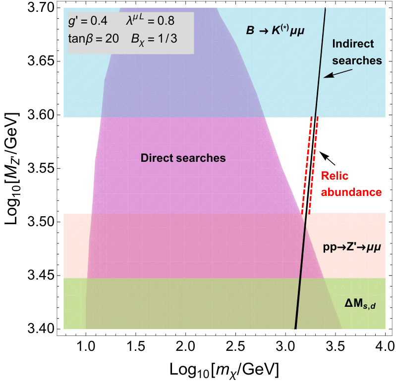
In Figure 2, we show the values of the and DM mass accommodating the observed DM relic abundance for the benchmark point considered. As observed earlier, the model can accommodate the DM relic abundance when the DM mass is near the pole due to the Wigner enhancement effect.
IV.2 Indirect Dark Matter detection
DM annihilations can also be probed by astronomical observations. Particularly interesting is the associated emission of photons (gamma rays). The phenomenology of such emission is trivial since these propagate in straight lines. The gamma ray flux per unit photon energy can be obtained by
| (58) |
This is a rather useful formula where the macroscopic and the microscopic physics are factorized out. On the one hand, the factor
| (59) |
quantifies the intrinsic usefulness of the observed region as target for indirect DM detection: l. o. s. stands for line of sight. On the other hand, the signal is also proportional to the “ability” for the DM to annihilate into photons. Quantitatively this is given by the cross section times the photon yield per annihilation channel (labelled with the letter in Equation 58).
Due to the simplicity of Equation 58 and the enormous progress in gamma-ray astronomy in recent years most of the studies in indirect DM detection are concerned with this messenger. In particular, dwarf spheroidal (dSph) galaxy observations by the Fermi Gamma-ray Space Telescope provide the up-to-date most stringent constraints on the annihilation cross section of DM in the sub-TeV mass region [64, 65]. Complementarily, observations by the HESS Telescope of the innermost parts of our Galaxy provide the strongest limits in the trans-TeV mass region [66].
We use therefore the limits reported in [64, 65, 66] in order to constrain the parameters of the model presented in this note. In doing this we only need the -channel annihilation rates at the center of mass energy . Relevant bounds on our model are derived from DM annihilation into fermion-antifermion channels, see Equation 52. Note that annihilations are suppressed in our model by the hard dependence of the parameter while the annihilation is kinematically suppressed close to the resonance. Off this resonance DM annihilation rates are too weak to be observed by the Fermi and HESS telescopes.
The strong limits that HESS puts on the and annihilation channels can be used to obtain exclusion regions. Notice that since the U(1)′ charges of third generation quarks are twice as large as the ones of the other two generations, the annihilation cross section into these two channels are by far the largest. In particular annihilations are such that , and for large masses near the resonance
| (60) |
independently of the couplings and .
In Fig. 2 indirect detection constraints on the model are also included. The models considered in the figure are better constrained by the HESS observation [66]. As evident in the figure, our indirect detection constraint is very narrow and quite sensitive to unaccounted-for effects. These include the radiative processes and halo velocity dispersion effects. However, at the quantitative level, these effects are negligible when compared with the uncertainties of the Galactic inner halo observed by the HESS Telescope.
Concretely, the indirect detection limits that result from considering factors ten times larger than the ones considered in [66] will exclude the models with the correct relic DM density. The latter are defined by the red dashed lines in Fig. 2. On the other hand, unrealistically shallower profiles ( factors three orders of magnitude smaller) than the ones considered in [66] would then be necessary for the DM in this model to be undetectable by indirect detection experiments.
IV.3 Direct detection of Dark Matter
Particles from the Milky Way DM halo can be detected in principle in terrestrial experiments if these interact with the SM. Direct detection experiments search for WIMP scattering off a target nucleus by identifying the associated nuclear recoil in a extremely low background environment. Typical recoil energies expected in these experiments are in the keV range [67].
At tree-level, the elastic scattering between a WIMP and a nucleus will be mediated in our model by the -channel exchange of a massive neutral vector boson with vectorial couplings to the DM candidate and to quarks (up to gauge mixing effects).
In order to compute the direct detection rates we match our model to an effective theory at the nuclear energy scale. Running effects from the symmetry breaking scale ( TeV) down to the nuclear scale ( GeV) have a small numerical impact in this model.55 5 We evaluate these effects following [68], using the code runDM [69]. At the nuclear energy scale our model generates dominant contributions to the standard spin-independent interaction to the nucleons ()
| (61) |
The latter is subject to a coherent enhancement in the nucleus, increasing the rate for direct detection searches. The spin-independent DM-nucleon cross section is given by
| (62) |
with being the DM-nucleon reduced mass.
The strongest limits on the spin-independent DM-nucleon cross section have been set by the Large Underground Xenon (LUX) experiment and by The Particle and Astrophysical Xenon Detector (PandaX). The latest bounds set by the LUX experiment are based on a dataset taken from September 2014 to May 2016 (332 live days) [70]. The limits from the PandaX-II experiment are very similar and are based on a combination of the dataset taken during the commissioning run (19.1 live days) and the first physics run taking place from March 9 to June 30, 2016 (79.6 live days) [71]. In Fig. 2 we show exclusion limits on the model parameter space derived from these searches. The limits are shown on the plane , fixing: , , and . We see that a large part of the allowed region left from flavour and collider bounds is excluded by direct DM searches. For larger values of , the derived constraints from direct searches basically exclude all the available parameter space shown in Fig. 2.
V Conclusions
Motivated by the observed departures from the Standard Model in decays, we have performed a comprehensive analysis of a family-dependent model featuring a Dirac fermion dark matter candidate. The simple model presented establishes a connection between dark matter stability and the hints of new physics in , with the boson acting as a portal between the dark sector and the Standard Model.
We found that the model can accommodate the current decay anomalies while satisfying flavour and collider constraints for a boson in the TeV range. For such a heavy mediator, we rely on the Wigner enhancement effect to achieve the right size of the dark matter annihilation cross section according to the current value of the dark matter relic abundance. Thus in our model, the dark matter candidate is in TeV range with . Fermi-LAT limits on dark matter annihilation from dwarf spheroidal galaxy observations exclude a very narrow, near-resonance, region of the model. In contrast, the latest limits from direct dark matter searches by the LUX and PandaX-II experiments severely constrain the available model parameter space.
Appendix A Details of the scalar sector
The complex Higgs doublets can be parametrized as
| (63) |
The complex scalar field can be similarly parametrized in terms of its real components
| (64) |
The scalar potential includes all terms invariant under the gauge symmetry. The charge of is constrained to be or in order to avoid a Goldstone boson in the spectrum. Additionally, we obtained that should be positive in order to accommodate data. We choose here . The scalar potential reads then
| (65) |
We assume that . After the gauge symmetry is spontaneously broken to the electromagnetic group, four degrees of freedom of the scalar fields give rise to the masses. The scalar spectrum contains three CP-even Higgs bosons , a CP-odd Higgs and a charged scalar . We perform a perturbative diagonalization in the small ratio as in [16]. In terms of the neutral components of the scalar fields, the CP-even physical states are
| (66) |
Here we assumed a decoupling scenario, with a light SM-like Higgs boson to be identified with the GeV boson and additional heavy scalars around the scale . In the CP-odd sector, we have the would-be Goldstone bosons giving mass to the and bosons and the CP-odd Higgs ,
| (67) |
The charged Higgs is given by
| (68) |
with giving the mass. The masses of the scalars are
| (69) |
The combination is given by
| (70) |
Acknowledgements.
The work of A.C. is supported by the Alexander von Humboldt Foundation. A.C. is grateful to the Mainz Institute for Theoretical Physics (MITP), the Università di Napoli Federico II and INFN for its hospitality and its partial support during the completion of this work. WZ.F. is grateful to Xiaoyong Chu, Zuowei Liu and Wei Xue for useful discussions. The work of M.V. was supported by DFG Cluster of Excelence “Origin and Structure of the Universe”. M.V. would like to thank the Theoretical Particle Physics group at the Ludwig-Maximilians-University of Munich and in particular Prof. Gerhard Buchalla’s group for their hospitality while essential contributions to this work were completed.References
- [1] R. Aaij et al. [LHCb Collaboration], Phys. Rev. Lett. 113 (2014) 151601 [arXiv:1406.6482 [hep-ex]].
- [2] G. Hiller and F. Kruger, Phys. Rev. D 69 (2004) 074020 [hep-ph/0310219].
- [3] A. Guevara, G. Lopez Castro, P. Roig and S. L. Tostado, Phys. Rev. D 92 (2015) no.5, 054035 [arXiv:1503.06890 [hep-ph]].
- [4] M. Bordone, G. Isidori and A. Pattori, arXiv:1605.07633 [hep-ph].
- [5] R. Alonso, B. Grinstein and J. Martin Camalich, Phys. Rev. Lett. 113 (2014) 241802 [arXiv:1407.7044 [hep-ph]].
- [6] D. Ghosh, M. Nardecchia and S. A. Renner, JHEP 1412, 131 (2014) [arXiv:1408.4097 [hep-ph]].
- [7] S. Jäger and J. Martin Camalich, Phys. Rev. D 93 (2016) no.1, 014028 [arXiv:1412.3183 [hep-ph]].
- [8] W. Altmannshofer and D. M. Straub, arXiv:1503.06199 [hep-ph].
- [9] S. Descotes-Genon, L. Hofer, J. Matias and J. Virto, JHEP 1606 (2016) 092 [arXiv:1510.04239 [hep-ph]].
- [10] M. Ciuchini, M. Fedele, E. Franco, S. Mishima, A. Paul, L. Silvestrini and M. Valli, JHEP 1606 (2016) 116 [arXiv:1512.07157 [hep-ph]].
- [11] T. Hurth, F. Mahmoudi and S. Neshatpour, Nucl. Phys. B 909 (2016) 737 [arXiv:1603.00865 [hep-ph]].
- [12] W. Altmannshofer, S. Gori, M. Pospelov and I. Yavin, Phys. Rev. D 89 (2014) 095033 [arXiv:1403.1269 [hep-ph]].
- [13] A. Crivellin, G. D’Ambrosio and J. Heeck, Phys. Rev. Lett. 114 (2015) 151801 [arXiv:1501.00993 [hep-ph]].
- [14] A. Crivellin, G. D’Ambrosio and J. Heeck, Phys. Rev. D 91 (2015) no.7, 075006 [arXiv:1503.03477 [hep-ph]].
- [15] D. Aristizabal Sierra, F. Staub and A. Vicente, Phys. Rev. D 92 (2015) no.1, 015001 [arXiv:1503.06077 [hep-ph]].
- [16] A. Celis, J. Fuentes-Martin, M. Jung and H. Serodio, Phys. Rev. D 92 (2015) no.1, 015007 [arXiv:1505.03079 [hep-ph]].
- [17] G. Belanger, C. Delaunay and S. Westhoff, Phys. Rev. D 92 (2015) 055021 [arXiv:1507.06660 [hep-ph]].
- [18] A. Falkowski, M. Nardecchia and R. Ziegler, JHEP 1511 (2015) 173 [arXiv:1509.01249 [hep-ph]].
- [19] B. Allanach, F. S. Queiroz, A. Strumia and S. Sun, Phys. Rev. D 93 (2016) no.5, 055045 [arXiv:1511.07447 [hep-ph]].
- [20] A. Celis, W. Z. Feng and D. Lüst, JHEP 1602 (2016) 007 [arXiv:1512.02218 [hep-ph]].
- [21] C. W. Chiang, X. G. He and G. Valencia, Phys. Rev. D 93 (2016) no.7, 074003 [arXiv:1601.07328 [hep-ph]].
- [22] S. M. Boucenna, A. Celis, J. Fuentes-Martin, A. Vicente and J. Virto, Phys. Lett. B 760 (2016) 214 [arXiv:1604.03088 [hep-ph]].
- [23] S. M. Boucenna, A. Celis, J. Fuentes-Martin, A. Vicente and J. Virto, arXiv:1608.01349 [hep-ph].
- [24] C. B. Jackson, G. Servant, G. Shaughnessy, T. M. P. Tait and M. Taoso, JCAP 1307 (2013) 021 [arXiv:1302.1802 [hep-ph]].
- [25] C. B. Jackson, G. Servant, G. Shaughnessy, T. M. P. Tait and M. Taoso, JCAP 1307 (2013) 006 [arXiv:1303.4717 [hep-ph]].
- [26] M. Duerr and P. Fileviez Perez, Phys. Lett. B 732 (2014) 101 [arXiv:1309.3970 [hep-ph]].
- [27] A. Alves, S. Profumo and F. S. Queiroz, JHEP 1404 (2014) 063 [arXiv:1312.5281 [hep-ph]].
- [28] G. Arcadi, Y. Mambrini, M. H. G. Tytgat and B. Zaldivar, JHEP 1403 (2014) 134 [arXiv:1401.0221 [hep-ph]].
- [29] W. Z. Feng, G. Shiu, P. Soler and F. Ye, JHEP 1405, 065 (2014) [arXiv:1401.5890 [hep-ph]].
- [30] N. F. Bell, Y. Cai, R. K. Leane and A. D. Medina, Phys. Rev. D 90 (2014) no.3, 035027 [arXiv:1407.3001 [hep-ph]].
- [31] M. Duerr and P. Fileviez Perez, Phys. Rev. D 91 (2015) no.9, 095001 [arXiv:1409.8165 [hep-ph]].
- [32] D. Hooper, Phys. Rev. D 91 (2015) 035025 [arXiv:1411.4079 [hep-ph]].
- [33] A. Alves, A. Berlin, S. Profumo and F. S. Queiroz, Phys. Rev. D 92 (2015) no.8, 083004 [arXiv:1501.03490 [hep-ph]].
- [34] M. Duerr, P. Fileviez Perez and J. Smirnov, Phys. Rev. D 92 (2015) no.8, 083521 [arXiv:1506.05107 [hep-ph]].
- [35] A. Alves, A. Berlin, S. Profumo and F. S. Queiroz, JHEP 1510 (2015) 076 [arXiv:1506.06767 [hep-ph]].
- [36] K. S. Babu, C. F. Kolda and J. March-Russell, Phys. Rev. D 57 (1998) 6788 [hep-ph/9710441].
- [37] S. Meinel and D. van Dyk, Phys. Rev. D 94, no. 1, 013007 (2016) [arXiv:1603.02974 [hep-ph]].
- [38] G. Aad et al. [ATLAS Collaboration], Phys. Rev. D 90, no. 5, 052005 (2014) [arXiv:1405.4123 [hep-ex]].
- [39] V. Khachatryan et al. [CMS Collaboration], JHEP 1504 (2015) 025 [arXiv:1412.6302 [hep-ex]].
- [40] The ATLAS collaboration, ATLAS-CONF-2016-045.
- [41] J. Alwall et al., JHEP 1407 (2014) 079 [arXiv:1405.0301 [hep-ph]].
- [42] CMS Collaboration, CMS-PAS-EXO-11-092.
- [43] A. Falkowski, D. M. Straub and A. Vicente, JHEP 1405 (2014) 092 [arXiv:1312.5329 [hep-ph]].
- [44] R. Dermisek, J. P. Hall, E. Lunghi and S. Shin, JHEP 1412, 013 (2014) [arXiv:1408.3123 [hep-ph]].
- [45] A. Lenz et al., Phys. Rev. D 83 (2011) 036004 [arXiv:1008.1593 [hep-ph]].
- [46] A. J. Buras, F. De Fazio, J. Girrbach and M. V. Carlucci, JHEP 1302 (2013) 023 [arXiv:1211.1237 [hep-ph]].
- [47] A. J. Buras, F. De Fazio and J. Girrbach, JHEP 1302 (2013) 116 [arXiv:1211.1896 [hep-ph]].
- [48] CKMfitter Group (J. Charles et al.), Eur. Phys. J. C41, 1-131 (2005) [hep-ph/0406184], updated results and plots available at: http://ckmfitter.in2p3.fr
- [49] A. Bazavov et al. [Fermilab Lattice and MILC Collaborations], arXiv:1602.03560 [hep-lat].
- [50] Y. Amhis et al. [Heavy Flavor Averaging Group (HFAG) Collaboration], arXiv:1412.7515 [hep-ex].
- [51] G. Hiller and M. Schmaltz, JHEP 1502 (2015) 055 [arXiv:1411.4773 [hep-ph]].
- [52] A. J. Buras, J. Girrbach-Noe, C. Niehoff and D. M. Straub, JHEP 1502 (2015) 184 doi:10.1007/JHEP02(2015)184 [arXiv:1409.4557 [hep-ph]].
- [53] J. P. Lees et al. [BaBar Collaboration], Phys. Rev. D 87 (2013) no.11, 112005 doi:10.1103/PhysRevD.87.112005 [arXiv:1303.7465 [hep-ex]].
- [54] O. Lutz et al. [Belle Collaboration], Phys. Rev. D 87 (2013) no.11, 111103 doi:10.1103/PhysRevD.87.111103 [arXiv:1303.3719 [hep-ex]].
- [55] G. Hiller and M. Schmaltz, Phys. Rev. D 90 (2014) 054014 [arXiv:1408.1627 [hep-ph]].
- [56] V. Khachatryan et al. [CMS and LHCb Collaborations], Nature 522 (2015) 68 [arXiv:1411.4413 [hep-ex]].
- [57] C. Bobeth, M. Gorbahn, T. Hermann, M. Misiak, E. Stamou and M. Steinhauser, Phys. Rev. Lett. 112 (2014) 101801 [arXiv:1311.0903 [hep-ph]].
- [58] M. Aaboud et al. [ATLAS Collaboration], arXiv:1604.04263 [hep-ex].
- [59] S. Weinberg, Phys. Rev. Lett. 43 (1979) 1566.
- [60] K. Griest and D. Seckel, Phys. Rev. D 43, 3191 (1991).
- [61] P. Gondolo and G. Gelmini, Nucl. Phys. B 360, 145 (1991).
- [62] P. Nath and R. L. Arnowitt, Phys. Rev. Lett. 70, 3696 (1993) [hep-ph/9302318].
- [63] M. Ibe, H. Murayama and T. T. Yanagida, Phys. Rev. D 79, 095009 (2009) [arXiv:0812.0072 [hep-ph]].
- [64] M. Ackermann et al. [Fermi-LAT Collaboration], Phys. Rev. Lett. 115 (2015) no.23, 231301 [arXiv:1503.02641 [astro-ph.HE]].
- [65] M. L. Ahnen et al. [MAGIC and Fermi-LAT Collaborations], JCAP 1602 (2016) no.02, 039 [arXiv:1601.06590 [astro-ph.HE]].
- [66] H. Abdallah et al. [HESS Collaboration], arXiv:1607.08142 [astro-ph.HE].
- [67] T. Marrodán Undagoitia and L. Rauch, J. Phys. G 43 (2016) no.1, 013001 [arXiv:1509.08767 [physics.ins-det]].
- [68] F. D’Eramo, B. J. Kavanagh and P. Panci, arXiv:1605.04917 [hep-ph].
- [69] F. D’Eramo, B. J. Kavanagh and P. Panci (2016). runDM (Version 1.0) [Computer software]. Available at https://github.com/bradkav/runDM/
- [70] D. S. Akerib et al. [LUX Collaboration], Phys. Rev. Lett. 118 (2017) no.2, 021303 doi:10.1103/PhysRevLett.118.021303 [arXiv:1608.07648 [astro-ph.CO]].
- [71] A. Tan et al. [PandaX-II Collaboration], arXiv:1607.07400 [hep-ex].