Channel Estimation for Diffusive Molecular Communications Thanks:  This paper was presented in part at the International Conference on Communications (ICC) 2016, Kuala Lumpur, Malaysia [31].Thanks: V. Jamali, A. Ahmadzadeh, and R. Schober are with the Institute for Digital Communications at the Friedrich-Alexander University (FAU), Erlangen, Germany (email: vahid.jamali@fau.de, arman.ahmadzadeh@fau.de, and robert.schober@fau.de).Thanks: C. Jardin and H. Sticht are with the Institute for Biochemistry at the Friedrich-Alexander University (FAU), Erlangen, Germany (email: christophe.jardin@fau.de and heinrich.sticht@fau.de).

The design of any communication system crucially depends on the characteristics of the channel under consideration. In MC systems, the impact of the channel on the number of observed molecules can be captured by the channel impulse response (CIR) which is defined as the expected number of molecules counted at the receiver at time $t$ after the instantaneous release of a known number of molecules by the transmitter at time $t=0$. The CIR, denoted by $\bar{c}(t)$, can be used as the basis for the design of equalization and detection schemes for MC systems [5, 6]. For diffusion-based MC, the released molecules move randomly according to Brownian motion which is caused by thermal vibration and collisions with other molecules in the fluid environment. Thereby, the average concentration of the molecules at a given coordinate $\mathbf{a}=[a_{x},a_{y},a_{z}]$ and at time $t$ after their release by the transmitter, denoted by $\bar{\mathcal{C}}(\mathbf{a},t)$, is governed by Fick’s second law of diffusion [5]. Finding $\bar{\mathcal{C}}(\mathbf{a},t)$ analytically involves solving partial differential equations and depends on initial and boundary conditions. Therefore, one possible approach for determining the CIR, which is widely employed in the literature [6], is to first derive a sufficiently accurate analytical expression for $\bar{\mathcal{C}}(\mathbf{a},t)$ for the considered MC channel from Fick’s second law, and to subsequently integrate it over the receiver volume, $V^{\mathtt{rec}}$, i.e.,

However, this approach may not be applicable in many practical scenarios as discussed in the following.

• •

  The CIR can be obtained based on (1) only for the special case of a fully transparent receiver where it is assumed that the molecules move through the receiver as if it was not present in the environment. The assumption of a fully transparent receiver is a valid approximation only for some particular scenarios where the interaction of the receiver with the molecules can be neglected. However, for general receivers, the relationship between the concentration $\bar{\mathcal{C}}(\mathbf{a},t)$ and the number of observed molecules $\bar{c}(t)$ may not be as straightforward [7, 8, 9].

• •

  Solving the differential equation associated with Fick’s second law is possible only for simple and idealistic environments. For example, assuming a point source located at the origin of an unbounded environment and impulsive molecule release, $\bar{\mathcal{C}}(\mathbf{a},t)$ is obtained as [6]

  $\displaystyle\bar{\mathcal{C}}(\mathbf{a},t)=\frac{N^{\mathtt{Tx}}}{\left(4\pi Dt\right)^{3/2}}\exp\left(-\frac{|\mathbf{a}|^{2}}{4Dt}\right)\quad\left[\frac{\text{\small molecules}}{\text{\small m}^{3}}\right],\,\,\,$

  (2)

  where $N^{\mathtt{Tx}}$ is the number of molecules released by the transmitter at $t=0$ and $D$ is the diffusion coefficient of the signaling molecule. However, $\bar{\mathcal{C}}(\mathbf{a},t)$ cannot be obtained in closed form for most practical MC environments which may involve difficult boundary conditions, non-instantaneous molecule release, flow, etc. Additionally, as has been shown in [10], the classical Fick’s diffusion equation might even not be applicable in complex MC environments as physico-chemical interactions of the molecules with other objects in the channel, such as other molecules, cells, and microvessels, are not accounted for.

• •

  Even if an expression for $\bar{\mathcal{C}}(\mathbf{a},t)$ can be obtained for a particular MC system, e.g. (2), it will be a function of several channel parameters such as the distance between the transmitter and the receiver and the diffusion coefficient. However, in practice, these parameters may not be known a priori and also have to be estimated [11, 12]. This complicates finding the CIR based on $\bar{\mathcal{C}}(\mathbf{a},t)$.

Fortunately, for most communication problems, including equalization and detection, only the expected number of molecules that the receiver observes at the sampling times is needed [5, 6]. Hence, the difficulties associated with deriving $\bar{\mathcal{C}}(\mathbf{a},t)$ can be avoided by directly estimating the CIR. Motivated by the above discussion, our goal in this paper is to develop a general CIR estimation framework for MC systems which is not limited to a particular MC channel model or a specific receiver type and does not require knowledge of the channel parameters.

In most existing works on MC, the CIR is assumed to be perfectly known for receiver design [5, 6, 13]. In the following, we review the relevant MC literature that focused on channel characterization. Estimation of the distance between a transmitter and a receiver was studied in [11, 14, 12] for diffusive MC. In [15], an end-to-end mathematical model, including transmitter, channel, and receiver, was presented, and in [16], a stochastic channel model was proposed for flow-based and diffusion-based MC. For active transport MC, a Markov chain channel model was derived in [17]. Additionally, a unifying model including the effects of external noise sources and inter-symbol interference (ISI) was proposed for diffusive MC in [18]. In [19], the authors analyzed a microfluidic MC channel, propagation noise, and channel memory. For neuro-spike communications, a physical model for the channel between two neurons was developed in [20]. In addition to these theoretical works, experimental results for the characterization of MC channels were reported in [21, 22]. However, the focus of [11, 12, 15, 16, 17, 18, 19, 20, 21, 22] is either channel modeling or the estimation of channel parameters, i.e., the obtained results are not directly applicable to CIR acquisition. In contrast to MC, for conventional wireless communication, there is a rich literature on channel estimation, mainly for linear channel models and impairment by additive white Gaussian noise (AWGN), see [23, 24, 25], and the references therein. Channel estimation was also studied for non-linear and/or non-AWGN channels especially in optical communication. For example, a linear time-invariant system with chi-squared noise was used in [26] to model the optical fiber channel. However, the MC channel model considered in this paper is different from the channel models considered in [23, 24, 25, 26], and hence, these results are not directly applicable to MC.

In this paper, we consider the Poisson channel which was introduced in [27, 28] for molecule-counting receivers in MC systems. The Poisson channel was previously used to model optical communication channels with photon-counting receivers, see [29] and the references therein. Moreover, the authors of a recent paper [30] adopted the Poisson channel model for non-line-of-sight (NLOS) optical wireless communication and proposed two different channel estimators. However, to the best of the authors’ knowledge, channel estimation for the Poisson MC channel was first considered in the conference version of this paper [31]. We note that the channel estimators developed in this paper for MC systems are different from the channel estimators presented in [30] for NLOS optical communications. Moreover, the estimators considered in [30] do not take into account the non-negativity of the CIR coefficients. In contrast, we have carefully considered this non-negativity constraint on the CIR coefficients in the proposed estimators. Finally, in contrast to [30], we assume that the mean of the noise is unknown and has to be estimated as well. Therefore, the results in [30] are not directly applicable to the MC channel considered in this paper.

In this paper, we directly estimate the CIR of the MC channel based on the channel output, i.e., the number of molecules observed at the receiver. In particular, we present a training-based CIR estimation framework which aims at estimating the CIR based on the detected number of molecules at the receiver due to the emission of a sequence of known numbers of molecules by the transmitter. Thereby, we consider the following two scenarios: i) Non-Bayesian CIR estimation where statistical CIR knowledge is not available or not exploited. For this case, we first derive the optimal maximum likelihood (ML) CIR estimator. Subsequently, we obtain the suboptimal least sum of square errors (LSSE) CIR estimator which entails a lower computational complexity than the ML estimator. Additionally, we derive the classical Cramer Rao (CR) bound which constitutes a lower bound on the estimation error variance of any unbiased estimator. ii) Bayesian CIR estimation where knowledge of the CIR statistics is available and exploited. Here, we first investigate maximum a posteriori (MAP) estimation as the optimal approach which requires full statistical knowledge of the MC channel. Subsequently, we derive the linear minimum mean square error (LMMSE) estimator for the case when only the first and second order statistics of the MC channel are available. Additionally, we derive the Bayesian CR bound as a generalization of the classical CR bound for estimators which exploit statistical channel knowledge. Finally, we study optimal and suboptimal training sequence designs for the considered MC system. Simulation results confirm the analysis and evaluate the performance of the proposed estimation techniques with respect to the corresponding CR lower bound.

We note that in contrast to the conference version [31], which studies only the case when statistical channel knowledge is not exploited, this paper also provides optimal and suboptimal CIR estimators, training sequence designs, and performance bounds for the case when statistical channel knowledge is exploited. Moreover, many of the extensive discussions, simulation results, and proofs provided in this paper are not included in [31].

The remainder of this paper is organized as follows. In Section II, some preliminaries and assumptions are presented and the classical and Bayesian CR bounds are derived. CIR estimators which do not require statistical channel knowledge are proposed in Section III, and CIR estimators which do take advantage of statistical channel knowledge are given in Section IV. In Section V, several different training sequence designs are presented. Numerical results are provided in Section VI, and conclusions are drawn in Section VII.

Notations: We use the following notations throughout this paper: $\mathbbmss{E}_{x}\{\cdot\}$ denotes expectation with respect to random variable (RV) $x$, $|\cdot|$ represents the cardinality of a set, and $[x]^{+}=\max\{0,x\}$. Bold capital and small letters are used to denote matrices and vectors, respectively. $\mathbf{1}$ and $\mathbf{0}$ are vectors whose elements are all ones and zeros, respectively, $\mathbf{I}$ denotes the identity matrix, $\mathbf{A}^{T}$ denotes the transpose of $\mathbf{A}$, $\|\mathbf{a}\|$ represents the norm of vector $\mathbf{a}$, $[\mathbf{A}]_{mn}$ denotes the element in the $m$-th row and $n$-th column of matrix $\mathbf{A}$, $\mathrm{tr}\{\mathbf{A}\}$ is the trace of matrix $\mathbf{A}$, $\mathrm{diag}\{\mathbf{a}\}$ denotes a diagonal matrix with the elements of vector $\mathbf{a}$ on its main diagonal, $\mathrm{vdiag}\{\mathbf{A}\}$ is a vector which contains the diagonal entries of matrix $\mathbf{A}$, $\mathrm{eig}\{\mathbf{A}\}$ is the set of eigen-values of matrix $\mathbf{A}$, $\mathbf{A}\succeq 0$ denotes a positive semidefinite matrix $\mathbf{A}$, and $\mathbf{a}\geq\mathbf{0}$ specifies that all elements of vector $\mathbf{a}$ are non-negative. Additionally, $\nabla^{2}_{\mathbf{a}\mathbf{a}}f(\mathbf{a})$ denotes the Hessian matrix of function $f(\mathbf{a})$ with respect to vector $\mathbf{a}$. Furthermore, $\mathrm{Poiss}(\lambda)$ denotes a Poisson RV with mean $\lambda$, $\mathrm{Bin}(n,p)$ denotes a binomial RV for $n$ trials and success probability $p$, and $\mathcal{N}\left(\mathbf{a},\mathbf{A}\right)$ denotes a multivariate normal RV with mean vector $\mathbf{a}$ and covariance matrix $\mathbf{A}$.

We consider an MC system consisting of a transmitter, a channel, and a receiver, see Fig. 1 a). At the beginning of each symbol interval, the transmitter releases a fraction of $N^{\mathtt{Tx}}$ molecules where $N^{\mathtt{Tx}}$ is the maximum number of molecules that the transmitter can release at once, i.e., concentration shift keying (CSK) is performed [2]. In this paper, we assume that the transmitter emits only one type of molecule. The released molecules propagate through the medium between the transmitter and the receiver. We assume that the movements of individual molecules are independent from each other. The receiver counts the number of observed molecules in each symbol interval. We note that this is a rather general model for the MC receiver which includes well-known receivers such as the transparent receiver [6], the absorbing receiver [7], and the reactive receiver [8].

Due to the memory of the MC channel, inter-symbol interference (ISI) occurs [18, 19], see Fig. 1 b). In particular, ISI-free communication is only possible if the symbol intervals are chosen sufficiently large such that the CIR fully decays to zero within one symbol interval which severely limits the transmission rate and results in an inefficient MC system design. Therefore, taking into account the effect of ISI, we assume the following input-output relation for the MC system

where $r[k]$ is the number of molecules detected at the receiver in symbol interval $k$, $L$ is the number of memory taps of the channel, and $c_{l}[k]$ is the number of molecules observed at the receiver in symbol interval $k$ due to the release of $s[k-l+1]N^{\mathtt{Tx}}$ molecules by the transmitter in symbol interval $k-l+1$, where $s[k]\in[0,1]$ is the transmitted symbol in symbol interval $k$. Thereby, $c_{l}[k]$ can be well approximated by a Poisson RV with mean $\bar{c}_{l}s[k-l+1]$, i.e., $c_{l}[k]\sim\mathrm{Poiss}\left(\bar{c}_{l}s[k-l+1]\right)$, see [27, 5]. Moreover, $c_{\mathtt{n}}[k]$ is the number of external noise molecules detected by the receiver in symbol interval $k$ but not released by the transmitter. Noise molecules may originate from interfering sources which employ the same type of molecule as the considered MC system. Hence, $c_{\mathtt{n}}[k]$ can also be modeled as a Poisson RV, i.e., $c_{\mathtt{n}}[k]\sim\mathrm{Poiss}\left(\bar{c}_{\mathtt{n}}\right)$, where $\bar{c}_{\mathtt{n}}=\mathbbmss{E}\left\{c_{\mathtt{n}}[k]\right\}$.

Unlike the conventional linear input-output model for channels with memory in wireless communication systems [23, 24], the channel model in (3) is not linear since $s[k-l+1]$ does not affect the observation $r[k]$ directly but via Poisson RV $c_{l}[k]$. However, the expectation of the received signal is linearly dependent on the transmitted signal, i.e.,

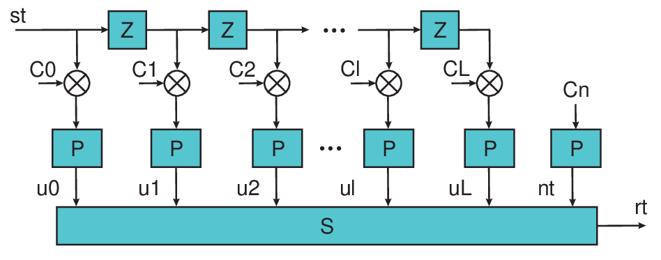
We note that for a given $s[k]$, in general, the actual number of molecules observed at the receiver, $r[k]$, will differ from the expected number of observed molecules, $\bar{r}[k]$, due to the intrinsic noisiness of diffusion. Here, we emphasize that the considered MC channel model is characterized by $\bar{c}_{l},\,\,l=1,\dots,L$, and $\bar{c}_{\mathtt{n}}$, see Fig. 2, which we refer to as the CIR of the MC channel throughout the the remainder of the paper.

Let $\mathbf{s}=[s[1],s[2],\dots,s[K]]^{T}$ be a training sequence of length $K$. Here, we assume continuous transmission. Therefore, in order to ensure that the received signal is only affected by training sequence $\mathbf{s}$ and not by the transmissions in previous symbol intervals, we only employ $r[k],\,\,k\geq L$, for CIR estimation. Thereby, the $K-L+1$ samples used for CIR estimation are given by

For convenience of notation, we define $\mathbf{r}=[r[L],r[L+1],\dots,r[K]]^{T}$ and $\bar{\mathbf{c}}=[\bar{c}_{1},\bar{c}_{2},\dots,\bar{c}_{L},\bar{c}_{\mathtt{n}}]^{T}$, and $f_{\mathbf{r}}(\mathbf{r}|\bar{\mathbf{c}},\mathbf{s})$ is the probability density function (PDF) of observation $\mathbf{r}$ conditioned on a given channel $\bar{\mathbf{c}}$ and a given training sequence $\mathbf{s}$. We assume that the CIR¹¹ 1 With a slight abuse of notation, we refer to vector $\bar{\mathbf{c}}$ as the CIR vector throughout the remainder of the paper although $\bar{\mathbf{c}}$ also contains the mean of the noise $\bar{c}_{\mathtt{n}}$., $\bar{\mathbf{c}}$, remains unchanged for a sufficiently large block of symbol intervals during which CIR estimation and data transmission are performed. However, the CIR may change from one block to the next due to e.g. a change of the distance between transmitter and receiver. To model this, we assume that CIR $\bar{\mathbf{c}}$ is a RV which takes its values in each block according to a PDF $f_{\bar{\mathbf{c}}}(\bar{\mathbf{c}})$. To summarize, in each block, the stochastic model in (3) is characterized by $\bar{\mathbf{c}}$ and our goal in this paper is to estimate $\bar{\mathbf{c}}$ based on the vector of random observations $\mathbf{r}$.

The classical CR bound is a lower bound on the variance of any unbiased estimator of a deterministic parameter. However, this bound can be also generalized to stochastic parameters which leads to the Bayesian CR bound [32, 33]. In particular, under some regularity conditions²² 2 These conditions ensure that the Fisher information matrix exists. In particular, the continuous differentiablity of the PDFs $f_{\mathbf{r}}(\mathbf{r}|\bar{\mathbf{c}},\mathbf{s})$ and $f_{\mathbf{r},\bar{\mathbf{c}}}(\mathbf{r},\bar{\mathbf{c}}|\mathbf{s})$ is a sufficient condition [32]., the covariance matrix of any unbiased estimate, $\hat{\bar{\mathbf{c}}}$, of parameter $\bar{\mathbf{c}}$, denoted by $\mathbf{C}(\hat{\bar{\mathbf{c}}})$, satisfies

where $\mathbf{I}\left(\bar{\mathbf{c}}\right)$ is the Fisher information matrix of parameter vector $\bar{\mathbf{c}}$ and is given by [33]

We assume that conditioned on $\bar{\mathbf{c}}$ and $\mathbf{s}$, the observations in different symbol intervals are independent, i.e., $r[k]$ is independent of $r[k^{\prime}]$ for $k\neq k^{\prime}$. This assumption is valid in practice if the time interval between two consecutive samples is sufficiently large, see [5] for a detailed discussion. Moreover, from (3), we observe that $r[k]$ is a sum of Poisson RVs. Hence, $r[k]$ is also a Poisson RV with its mean equal to the sum of the means of the summands, i.e., $r[k]\sim\mathrm{Poiss}(\bar{r}[k])$ with $\bar{r}[k]=\bar{c}_{\mathtt{n}}+\sum_{l=1}^{L}\bar{c}_{l}s[k-l+1]=\bar{\mathbf{c}}^{T}\mathbf{s}_{k}$ and $\mathbf{s}_{k}=[s[k],s[k-1],\dots,s[k-L+1],1]^{T}$. Therefore, $f_{\mathbf{r}}(\mathbf{r}|\bar{\mathbf{c}},\mathbf{s})$ is given by

For a positive semidefinite matrix, the diagonal elements are non-negative, i.e., $\big[\mathbf{C}(\hat{\bar{\mathbf{c}}})-\mathbf{I}^{-1}\left(\bar{\mathbf{c}}\right)\big]_{i,i}\geq 0$. Therefore, for an unbiased estimator, i.e., $\mathbbmss{E}\left\{\hat{\bar{\mathbf{c}}}\right\}=\bar{\mathbf{c}}$ holds, with the estimation error vector defined as $\mathbf{e}=\bar{\mathbf{c}}-\hat{\bar{\mathbf{c}}}$, the classical CR bound for deterministic $\bar{\mathbf{c}}$ provides the following lower bound on the sum of the expected square errors

where $\mathtt{CCRB}(\bar{\mathbf{c}})$ denotes the classical CR bound for a given fixed/deterministic parameter $\bar{\mathbf{c}}$.

On the other hand, the Bayesian CR bound for stochastic $\bar{\mathbf{c}}$ is given by

The expectation in (12) is taken over RV $\bar{\mathbf{c}}$ which takes its values according to PDF $f_{\bar{\mathbf{c}}}(\bar{\mathbf{c}})$. Note that $f_{\bar{\mathbf{c}}}(\bar{\mathbf{c}})$ depends on the MC environment and a general analytical expression for $f_{\bar{\mathbf{c}}}(\bar{\mathbf{c}})$ is not yet available in the literature. In practice, $f_{\bar{\mathbf{c}}}(\bar{\mathbf{c}})$ can be obtained using historical measurements of the CIR, see Remark 8 for further discussion.

The ML CIR estimator finds the CIR estimate which maximizes the likelihood of observation vector $\mathbf{r}$ [32]. In particular, the ML estimator is given by

where $f_{\mathbf{r}}(\mathbf{r}|\bar{\mathbf{c}},\mathbf{s})$ is given in (10). Maximizing $f_{\mathbf{r}}(\mathbf{r}|\bar{\mathbf{c}},\mathbf{s})$ is equivalent to maximizing $\mathrm{ln}(f_{\mathbf{r}}(\mathbf{r}|\bar{\mathbf{c}},\mathbf{s}))$ since $\mathrm{ln}(\cdot)$ is a monotonically increasing function. Hence, the ML estimate can be rewritten as

To present the solution of the above optimization problem rigorously, we first define some auxiliary variables. Let $\mathcal{A}=\{\mathcal{A}_{1},\mathcal{A}_{2},\dots,\mathcal{A}_{N}\}$ denote a set which contains all possible $N=2^{L+1}-1$ subsets of set $\mathcal{F}=\{1,2,\cdots,L,\mathtt{n}\}$ except for the empty set. Here, $\mathcal{A}_{n},\,\,n=1,2,\dots,N$, denotes the $n$-th subset of $\mathcal{A}$. Moreover, let $\bar{\mathbf{c}}^{\mathcal{A}_{n}}$ and $\mathbf{s}_{k}^{\mathcal{A}_{n}}$ denote reduced-dimension versions of $\bar{\mathbf{c}}$ and $\mathbf{s}_{k}$, respectively, which contain only those elements of $\bar{\mathbf{c}}$ and $\mathbf{s}_{k}$ whose indices are elements of set $\mathcal{A}_{n}$, respectively.

The LSSE CIR estimator chooses that $\bar{\mathbf{c}}$ which minimizes the sum of the square errors for observation vector $\mathbf{r}$. Thereby, the error vector is defined as $\bm{\epsilon}=\mathbf{r}-\mathbbmss{E}\left\{\mathbf{r}\right\}=\mathbf{r}-\mathbf{S}\bar{\mathbf{c}}$ where $\mathbf{S}=[\mathbf{s}_{L},\mathbf{s}_{L+1},\dots,\mathbf{s}_{K}]^{T}$. In particular, the LSSE CIR estimate can be formally written as

Here, the square norm of the error vector is obtained as

where we used the following properties of the trace: $\mathrm{tr}\left\{\mathbf{A}\right\}=\mathrm{tr}\left\{\mathbf{A}^{T}\right\}$ and $\mathrm{tr}\left\{\mathbf{A}\mathbf{B}\right\}=\mathrm{tr}\left\{\mathbf{BA}\right\}$ [35]. The LSSE estimate is given in the following lemma where we use the auxiliary matrix $\mathbf{S}^{\mathcal{A}_{n}}=[\mathbf{s}_{L}^{\mathcal{A}_{n}},\mathbf{s}_{L+1}^{\mathcal{A}_{n}},\dots,\mathbf{s}_{K}^{\mathcal{A}_{n}}]^{T}$.

The MAP CIR estimator is the optimal estimator assuming that full statistical knowledge of the MC channel is available, i.e., $f_{\bar{\mathbf{c}}}(\bar{\mathbf{c}})$. In particular, the MAP CIR estimator chooses that CIR $\bar{\mathbf{c}}$ which maximizes the posterior expected value of observation vector $\mathbf{r}$, i.e., $f_{\bar{\mathbf{c}}}(\bar{\mathbf{c}}|\mathbf{r},\mathbf{s})$. Thereby, the MAP estimate is given by

where $(a)$ follows the Bayes’ Theorem [32]. Note that the term $f_{\mathbf{r}}(\mathbf{r})$ does not depend on the estimate $\bar{\mathbf{c}}$. Moreover, considering that $\mathrm{ln}(\cdot)$ is a monotonically increasing function, the MAP estimate can be rewritten in the following convenient form

where $g(\bar{\mathbf{c}})$ is given in (14).

Similar to the ML and LSSE estimates provided in the previous section, the optimal MAP estimate is either a stationary point or a boundary point, see Algorithm 1. Here, we do not provide a detailed solution for the MAP estimate due to space constraints, instead, we highlight the main steps for the case when the solution is a stationary point. For the case when the solution is a boundary point, we can employ the same methodology as in Algorithm 1 to find $\hat{\bar{\mathbf{c}}}^{\mathtt{MAP}}$. In particular, the stationary points of the cost function in (22) are obtained by equating its derivative to zero, i.e., $\frac{\partial g(\bar{\mathbf{c}})}{\partial\bar{\mathbf{c}}}+\frac{\partial\mathrm{ln}\left(f_{\bar{\mathbf{c}}}(\bar{\mathbf{c}})\right)}{\partial\bar{\mathbf{c}}}=\mathbf{0}$. Note that the first term $\frac{\partial g(\bar{\mathbf{c}})}{\partial\bar{\mathbf{c}}}$ is given on the left-hand side of (15) for $\mathcal{A}_{n}=\mathcal{F}$ and the second term is given by $\frac{\partial\mathrm{ln}\left(f_{\bar{\mathbf{c}}}(\bar{\mathbf{c}})\right)}{\partial\bar{\mathbf{c}}}=-\frac{1}{2}\left(\bm{\Phi}_{\bar{\mathbf{c}}\bar{\mathbf{c}}}^{-1}+\bm{\Phi}_{\bar{\mathbf{c}}\bar{\mathbf{c}}}^{-T}\right)(\bar{\mathbf{c}}-\bm{\mu}_{\bar{\mathbf{c}}})$ for the considered Gaussian PDF $f_{\bar{\mathbf{c}}}(\bar{\mathbf{c}})$. We note that although the complexity of the MAP estimator may not be affordable for practical MC systems, we can still use it as a benchmark scheme to evaluate the performance of less complex estimators, e.g., the LMMSE estimator.

The MAP estimator in (22) requires full knowledge of the channel statistics, i.e., $f_{\bar{\mathbf{c}}}(\bar{\mathbf{c}})$, which is difficult to obtain for practical MC channels, cf Remark 8. Therefore, in the following, we consider an LMMSE-based estimator which requires only knowledge of the first and second order statistics of the MC channel. In particular, in estimation theory, the average square norm of the estimation error $\mathbf{e}=\bar{\mathbf{c}}-\hat{\bar{\mathbf{c}}}$ is often adopted as performance metric, i.e., $\mathbbmss{E}\left\{\|\mathbf{e}\|^{2}\right\}$. Therefore, one can design an LMMSE estimator which directly minimizes $\mathbbmss{E}\left\{\|\mathbf{e}\|^{2}\right\}$. We note that the estimation error has to be averaged over both $\mathbf{r}$ and $\bar{\mathbf{c}}$, i.e., $\mathbbmss{E}_{\mathbf{r},\bar{\mathbf{c}}}\left\{\|\mathbf{e}\|^{2}\right\}$, since both are randomly changing, and hence, have to be modeled as RVs. In this paper, we consider an LMMSE-based estimator given by $\hat{\bar{\mathbf{c}}}^{\mathtt{MMSE}}=\left[\mathbf{F}^{\mathtt{MMSE}}\mathbf{r}\right]^{+}$ where $\mathbf{F}^{\mathtt{MMSE}}$ is the MMSE matrix. Moreover, for mathematical tractability, we optimize $\mathbf{F}^{\mathtt{MMSE}}$ such that an upper bound on the estimation error is minimized, i.e.,

where $\mathbf{e}^{\mathtt{MMSE}}_{\mathtt{up}}=\bar{\mathbf{c}}-\hat{\bar{\mathbf{c}}}^{\mathtt{MMSE}}_{\mathtt{up}}$ and $\hat{\bar{\mathbf{c}}}^{\mathtt{MMSE}}_{\mathtt{up}}=\mathbf{F}^{\mathtt{MMSE}}\mathbf{r}$. Note that $\hat{\bar{\mathbf{c}}}^{\mathtt{MMSE}}_{\mathtt{up}}$ yields an upper bound on the estimation error of $\hat{\bar{\mathbf{c}}}^{\mathtt{MMSE}}$ because we neglect the side information that the CIR coefficients have to be non-negative by dropping $[\cdot]^{+}$. Hereby, $\mathbbmss{E}_{\mathbf{r},\bar{\mathbf{c}}}\left\{\|\mathbf{e}^{\mathtt{MMSE}}_{\mathtt{up}}\|^{2}\right\}$ is obtained as

where

and $\bm{\mu}_{\bar{\mathbf{c}}}=\mathbbmss{E}_{\bar{\mathbf{c}}}\{\bar{\mathbf{c}}\}$ and $\bm{\Phi}_{\bar{\mathbf{c}}\bar{\mathbf{c}}}=\mathbbmss{E}_{\bar{\mathbf{c}}}\left\{\bar{\mathbf{c}}\bar{\mathbf{c}}^{T}\right\}$. In addition, in (25aa) and (25ab), we use $\mathbbmss{E}_{\mathbf{X}}\left\{\mathrm{tr}\left\{\mathbf{AXB}\right\}\right\}=\mathrm{tr}\left\{\mathbf{A}\mathbbmss{E}_{\mathbf{X}}\left\{\mathbf{X}\right\}\mathbf{B}\right\}$, which holds for general matrices $\mathbf{A}$, $\mathbf{B}$, and $\mathbf{X}$. Furthermore, in (25aa), we use $\mathbbmss{E}_{\mathbf{x}}\left\{\mathbf{x}\mathbf{x}^{T}\right\}=\bm{\lambda}\bm{\lambda}^{T}+\mathrm{diag}\{\bm{\lambda}\}$, which is valid for multivariate Poisson random vectors $\mathbf{x}$ with covariance matrix $\mathbf{C}(\mathbf{x})=\mathrm{diag}\{\bm{\lambda}\}$. The optimal MMSE matrix is given in the following lemma.

We first consider a training sequence design which minimizes an upper bound on the average estimation error of the LSSE estimator. First, we note that for training sequence design, the estimation error has to be averaged over both $\mathbf{r}$ and $\bar{\mathbf{c}}$ since both are a priori unknown, and hence, have to be modeled as RVs. Again, we recall that in the system model, we assumed a priori $L$ non-zero taps and a noise with non-zero mean. Therefore, neglecting the information that $\bar{\mathbf{c}}\geq\mathbf{0}$ has to hold in (17) yields an upper bound on the estimation error for the LSSE estimator. This upper bound is adopted here for the problem of sequence design since the solution of (17) after dropping constraint $\bar{\mathbf{c}}\geq\mathbf{0}$ leads to the simple and elegant closed-form solution $\hat{\bar{\mathbf{c}}}^{\mathtt{LSSE}}_{\mathtt{up}}=\left(\mathbf{S}^{T}\mathbf{S}\right)^{-1}\mathbf{S}\mathbf{r}$, which we can employ to find optimal training sequences. Moreover, this upper bound is tight as $K\to\infty$ since $\hat{\bar{\mathbf{c}}}^{\mathtt{LSSE}}>\mathbf{0}$ holds and we obtain $\hat{\bar{\mathbf{c}}}^{\mathtt{LSSE}}=\hat{\bar{\mathbf{c}}}^{\mathtt{LSSE}}_{\mathtt{up}}$. In Section VI, Fig. 8, we show numerically that even for short sequence lengths, this upper bound is not loose.

Defining the estimation error as $\mathbf{e}^{\mathtt{LSSE}}_{\mathtt{up}}=\bar{\mathbf{c}}-\hat{\bar{\mathbf{c}}}^{\mathtt{LSSE}}_{\mathtt{up}}$, the expected square error norm is obtained as

Next, we calculate the expectation with respect to $(\mathbf{r},\bar{\mathbf{c}})$ in (28) in two steps, namely first with respect to $\mathbf{r}$ conditioned on $\bar{\mathbf{c}}$ and then with respect to $\bar{\mathbf{c}}$. Exploiting $\mathbbmss{E}_{\mathbf{X}}\left\{\mathrm{tr}\left\{\mathbf{AXB}\right\}\right\}=\mathrm{tr}\left\{\mathbf{A}\mathbbmss{E}_{\mathbf{X}}\left\{\mathbf{X}\right\}\mathbf{B}\right\}$ and $\mathbbmss{E}_{\mathbf{x}}\left\{\mathbf{x}\mathbf{x}^{T}\right\}=\bm{\lambda}\bm{\lambda}^{T}+\mathrm{diag}\{\bm{\lambda}\}$, $\mathbbmss{E}\left\{\|\mathbf{e}^{\mathtt{LSSE}}_{\mathtt{up}}\|^{2}\right\}$ can be calculated as

The evaluation of the expression in (29) can be numerically challenging due to the required inversion of matrix $\mathbf{S}^{T}\mathbf{S}$, especially when one of the eigen-values of $\mathbf{S}^{T}\mathbf{S}$ is close to zero. One way to cope with this problem is to eliminate all sequences resulting in close-to-zero eigen-values for matrix $\mathbf{S}^{T}\mathbf{S}$ during the search. Formally, we can adopt the following search criterion for LSSE-based training sequence design

where $\widetilde{\mathcal{S}}=\left\{\mathbf{s}\in\mathcal{S}^{K}\big||x|>\varepsilon,\,\,\,\,\forall x\in\mathrm{eig}\left\{\mathbf{S}^{T}\mathbf{S}\right\}\right\}$ and $\varepsilon$ is a small number which guarantees that the eigen-values of matrix $\mathbf{S}^{T}\mathbf{S}$ are not close to zero, e.g., in Section VI, we choose $\varepsilon=10^{-9}$.

Similar to the LSSE-based sequence design, the LMMSE estimate $\hat{\bar{\mathbf{c}}}^{\mathtt{MMSE}}$ in Lemma 3 can be used as the basis for sequence design. In this paper, we choose the optimal LMMSE-based training sequence such that the upper bound on the MMSE estimation error is minimized, i.e., $\mathbbmss{E}_{\mathbf{r},\bar{\mathbf{c}}}\left\{\|\mathbf{e}^{\mathtt{MMSE}}_{\mathtt{up}}\|^{2}\right\}$ in (24). In particular, substituting $\mathbf{F}^{\mathtt{MMSE}}$ in (27) into (24), simplifying the resulting expression for $\mathbbmss{E}_{\mathbf{r},\bar{\mathbf{c}}}\left\{\|\mathbf{e}^{\mathtt{MMSE}}_{\mathtt{up}}\|^{2}\right\}$, and removing the terms which do not depend on the sequence, we obtain the following criterion for the optimal LMMSE-based training sequence

References

- [1] T. Nakano, M. Moore, F. Wei, A. Vasilakos, and J. Shuai, “Molecular Communication and Networking: Opportunities and Challenges,” IEEE Trans. NanoBiosci, vol. 11, no. 2, pp. 135–148, Jun. 2012.
- [2] N. Farsad, H. Yilmaz, A. Eckford, C. Chae, and W. Guo, “A Comprehensive Survey of Recent Advancements in Molecular Communication,” IEEE Commun. Surveys Tutorials, vol. PP, no. 99, pp. 1–1, 2016.
- [3] I. Akyildiz, F. Brunetti, and C. Blazquez, “Nanonetworks: A New Communication Paradigm,” Comput. Net., vol. 52, pp. 2260–2279, Apr. 2008.
- [4] B. Alberts, D. Bray, K. Hopkin, A. Johnson, J. Lewis, M. Raff, K. Roberts, and P. Walter, Essential Cell Biology. Garland Science, 4th ed., 2014.
- [5] A. Noel, K. Cheung, and R. Schober, “Optimal Receiver Design for Diffusive Molecular Communication with Flow and Additive Noise,” IEEE Trans. NanoBiosci., vol. 13, no. 3, pp. 350–362, Sept. 2014.
- [6] M. Mahfuz, D. Makrakis, and H. Mouftah, “A Comprehensive Study of Sampling-Based Optimum Signal Detection in Concentration-Encoded Molecular Communication,” IEEE Trans. NanoBiosci., vol. 13, no. 3, pp. 208–222, Sept. 2014.
- [7] A. Akkaya, H. Yilmaz, C. Chae, and T. Tugcu, “Effect of Receptor Density and Size on Signal Reception in Molecular Communication via Diffusion With an Absorbing Receiver,” IEEE Commun. Lett., vol. 19, no. 2, pp. 155–158, Feb. 2015.
- [8] A. Ahmadzadeh, H. Arjmandi, A. Burkovski, and R. Schober, “Reactive Receiver Modeling for Diffusive Molecular Communication Systems with Molecule Degradation,” in Proc. IEEE ICC, Kuala Lumpur, May 2016, pp. 1–7.
- [9] H. Yilmaz, A. Heren, T. Tugcu, and C. B. Chae, “Three-Dimensional Channel Characteristics for Molecular Communications With an Absorbing Receiver,” IEEE Commun. Lett., vol. 18, no. 6, pp. 929–932, Jun. 2014.
- [10] G. Wei and R. Marculescu, “Miniature Devices in the Wild: Modeling Molecular Communication in Complex Extracellular Spaces,” IEEE J. Select. Areas Commun., vol. 32, no. 12, pp. 2344–2353, Dec. 2014.
- [11] M. Moore, T. Nakano, A. Enomoto, and T. Suda, “Measuring Distance From Single Spike Feedback Signals in Molecular Communication,” IEEE Trans. Sig. Process., vol. 60, no. 7, pp. 3576–3587, Jul. 2012.
- [12] A. Noel, K. Cheung, and R. Schober, “Bounds on Distance Estimation via Diffusive Molecular Communication,” in IEEE Globecom, Dec. 2014, pp. 2813–2819.
- [13] A. Ahmadzadeh, A. Noel, A. Burkovski, and R. Schober, “Amplify-and-Forward Relaying in Two-Hop Diffusion-Based Molecular Communication Networks,” in Proc. IEEE Globecom, San Diego, Dec 2015, pp. 1–7.
- [14] X. Wang, M. Higgins, and M. Leeson, “Distance Estimation Schemes for Diffusion Based Molecular Communication Systems,” IEEE Commun. Lett., vol. 19, no. 3, pp. 399–402, Mar. 2015.
- [15] M. Pierobon and I. Akyildiz, “A Physical End-to-End Model for Molecular Communication in Nanonetworks,” IEEE J. Sel. Areas Commun., vol. 28, no. 4, pp. 602–611, May 2010.
- [16] D. Miorandi, “A Stochastic Model for Molecular Communications,” Nano Commun. Netw., vol. 2, no. 4, pp. 205–212, 2011.
- [17] N. Farsad, A. Eckford, and S. Hiyama, “A Markov Chain Channel Model for Active Transport Molecular Communication,” IEEE Trans. Signal. Process., vol. 62, no. 9, pp. 2424–2436, May 2014.
- [18] A. Noel, K. Cheung, and R. Schober, “A Unifying Model for External Noise Sources and ISI in Diffusive Molecular Communication,” IEEE J. Sel. Areas Commun., vol. 32, no. 12, pp. 2330–2343, Dec. 2014.
- [19] A. Bicen and I. Akyildiz, “End-to-End Propagation Noise and Memory Analysis for Molecular Communication over Microfluidic Channels,” IEEE Trans. Commun., vol. 62, no. 7, pp. 2432–2443, Jul. 2014.
- [20] E. Balevi and O. Akan, “A Physical Channel Model for Nanoscale Neuro-Spike Communications,” IEEE Trans. Commun., vol. 61, no. 3, pp. 1178–1187, Mar. 2013.
- [21] N. Farsad, N.-R. Kim, A. Eckford, and C. B. Chae, “Channel and Noise Models for Nonlinear Molecular Communication Systems,” IEEE J. Select. Areas Commun., vol. 32, no. 12, pp. 2392–2401, Dec. 2014.
- [22] A. Biral, D. Zordan, and A. Zanella, “Modeling, Simulation and Experimentation of Droplet-Based Microfluidic Networks,” IEEE Trans. Molecular, Biol., and Multi-Scale Commun., vol. 1, no. 2, pp. 122–134, Jun. 2015.
- [23] S. Crozier, D. Falconer, and S. Mahmoud, “Least Sum of Squared Errors (LSSE) Channel Estimation,” IEE Proc. F Radar Sig. Process., vol. 138, no. 4, pp. 371–378, Aug. 1991.
- [24] M. Ozdemir and H. Arslan, “Channel Estimation for Wireless OFDM Systems,” IEEE Commun. Surveys Tutorials, vol. 9, no. 2, pp. 18–48, 2007.
- [25] Y. Liu, Z. Tan, H. Hu, L. Cimini, and G. Li, “Channel Estimation for OFDM,” IEEE Commun. Surveys Tutorials, vol. 16, no. 4, pp. 1891–1908, 2014.
- [26] C. Yang, F. Yang, and Z. Wang, “Clustering-Based Adaptive Channel Estimator for Optical Fiber Communication Systems,” IEEE Photonics Technol. Lett., vol. 20, no. 20, pp. 1670–1672, Oct. 2008.
- [27] H. Arjmandi, A. Gohari, M. Kenari, and F. Bateni, “Diffusion-Based Nanonetworking: A New Modulation Technique and Performance Analysis,” IEEE Commun. Lett., vol. 17, no. 4, pp. 645–648, Apr. 2013.
- [28] R. Mosayebi, H. Arjmandi, A. Gohari, M. Nasiri-Kenari, and U. Mitra, “Receivers for Diffusion-Based Molecular Communication: Exploiting Memory and Sampling Rate,” IEEE J. Sel. Areas Commun., vol. 32, no. 12, pp. 2368–2380, Dec. 2014.
- [29] D. Guo, S. Shamai, and S. Verdu, “Mutual Information and Conditional Mean Estimation in Poisson Channels,” IEEE Trans. Inf. Theory, vol. 54, no. 5, pp. 1837–1849, May 2008.
- [30] C. Gong and Z. Xu, “Channel Estimation and Signal Detection for Optical Wireless Scattering Communication with Inter-Symbol Interference,” IEEE Trans. Wireless Commun., vol. 14, no. 10, pp. 5326–5337, Oct. 2015.
- [31] V. Jamali, A. Ahmadzadeh, C. Jardin, C. Sticht, and R. Schober, “Channel Estimation Techniques for Diffusive Molecular Communications,” in Proc. IEEE ICC, Kuala Lumpur, May 2016, pp. 1–7.
- [32] A. Gelman, J. B. Carlin, H. S. Stern, and D. B. Rubin, Bayesian Data Analysis. Taylor & Francis, 2014, vol. 2.
- [33] H. L. Van Trees, Detection, Estimation, and Modulation Theory. John Wiley & Sons, 2004.
- [34] M. D. Perlman, “Jensen’s Inequality for a Convex Vector-Valued Function on an Infinite-Dimensional Space,” J. Multivariate Anal., vol. 4, no. 1, pp. 52–65, 1974.
- [35] P. H. Schonemann, “On the Formal Differentiation of Traces and Determinants,” Multivariate Behavioral Research, vol. 20, no. 2, pp. 113–139, 1985.
- [36] S. Boyd and L. Vandenberghe, Convex Optimization. Cambridge, U.K.: Cambridge Univ. Press, 2004.
- [37] H. White, “A Heteroskedasticity-Consistent Covariance Matrix Estimator and a Direct Test for Heteroskedasticity,” Econometrica, vol. 48, no. 4, pp. 817–838, 1980. [Online]. Available: http://www.jstor.org/stable/1912934
- [38] G. Milne, “Response of the Ordinary Least Squares Estimator (OLS) to Deterministic and Stochastic Noise,” in IEEE AFRICON, vol. 2, Sept. 1996, pp. 1099–1104.