Minority spin dynamics in non-homogeneous Ising model: diverging timescales and exponents
Abstract
We investigate the dynamical behaviour of the Ising model under a zero temperature quench with the initial fraction of up spins . In one dimension, the known results for persistence probability are verified; it shows algebraic decay for both up and down spins asymptotically with different exponents. It is found that the conventional finite size scaling is valid here. In two dimensions however, the persistence probabilities are no longer algebraic; in particular for , persistence for the up (minority) spins shows the behaviour with time , while for the down (majority) spins, approaches a finite value. We find that the timescale diverges as , where and . The exponent varies as where is very close to the persistence exponent in two dimensions; . The results in two dimensions can be understood qualitatively by studying the exit probability, which for different system size is found to have the form , with . This result suggests that , where is an exponent not explored earlier.
pacs
89.75.Da, 89.65.-s, 64.60.De, 75.78.FgI Introduction
Dynamical phenomena associated with the ordering process of spin systems have been studied since a long time. While the domain growth and behaviour of correlation functions were the original issues of interest [1, 2], other phenomena like persistence and its variants have been extensively studied more recently [3, 4]. It is indeed astonishing to note that even after decades of research on these topics, newer features have been revealed. For example, in the zero temperature quenching dynamics of Ising model, frozen states [5, 6] and blinkers [7, 8, 9, 10] as nonequilibrium steady states have been shown to occur in dimensions greater than one. Recent studies of the zero temperature quenching dynamics in the two dimensional Ising model indicated that the domain growth behaviour can be explained in the framework of percolation theory [11, 12, 13]. Different ways of employing the zero temperature quench have also been explored in some very recent works in the Ising model [14, 15, 16]. Models with more complicated interactions with binary spin variables have often indicated the existence of dynamical universality classes other than the simple Ising model even in one dimension [17].
Prior to the discovery of the persistence phenomena [3] in the Ising and other spin models, it was believed that there is only one dynamical exponent which governs the behaviour of the system during the ordering dynamics. The persistence probability showed a power law decay with an exponent which could not be related to other known static or dynamic exponents. This indicated that there is a second independent dynamic exponent. Since the domain size and persistence show power law behaviour, there is essentially no timescale associated with these quantities. Physically this means that there are finite probabilities existing even at very large timescales. On the other hand, diverging timescales can be associated with dynamical behaviour close to the critical point. The typical relaxation behaviour of the order parameter as a function of time is exponential close to the critical temperature: , with diverging as the critical temperature is approached.
In the present work, we consider the zero temperature single spin flip Glauber dynamics of Ising model with nearest neighbour interaction when the initial configuration is non-homogeneous, i.e. the fraction of up and down spins are different. is the fraction of up spins ranging between and . is the homogeneous case and due to up/down spin symmetry, it is sufficient to take . The spins are otherwise uncorrelated. Three types of persistence behaviour is studied: (persistence for up spins), (persistence for down spins) and (persistence for the total system). The exact expression for the variation of the above mentioned quantities are known in one dimension in the thermodynamic limit. We have numerically evaluated the persistence probabilities for finite systems and checked that the familiar finite size scaling [18, 19] is valid for all values of . Our main results are for the two dimensional model, here we have numerically obtained the behaviour of , and and find the presence of a diverging timescale associated with or , whichever corresponds to the initial minority.
Another quantity associated with the ordering process that has been studied quite intensely in recent years is the exit probability. As a function of (the initial fraction of up spins), the exit probability is defined as the probability that the final state comprises all up spins. The behaviour of the exit probability helps in understanding qualitatively the persistence probability in the Ising model. Hence we have also conducted a detailed study of the exit probability in two dimensions to gain more insight into the problem.
In the next two sections, the results for one and two dimensionsal Ising model are discussed respectively. In the last section, summary and some discussions are presented.
II Results in one dimension and finite size scaling
For systems with non-uniform initial condition i.e. with unequal initial fraction of up and down spins, the exact result for the Ising model in one dimension shows that the density of persistent spins decays algebraically as [20]
| (1) |
The exponents are different for the up and down spins;
| (2) |
where is the initial concentration of up (down) spins. For equal initial fraction of up and down spins (i.e. for ) we have [3]. In this paper we follow the notation unless otherwise specified.
During the coarsening, the typical domain size shows a power-law growth with time:
| (3) |
being the domain growth exponent. For the Ising model in all dimensions [1].
While the persistence exponents are dependent, the domain growth exponent is identical for all . This is easy to explain. Consider, e.g. the growth phenomena for . Immediately after the time evolution starts, will attain a different value. One might as well consider this to be the initial state, hence for all [1, 2].
In one dimension, it is known that for the homogeneous case, the persistence probability obeys finite size scaling. The behaviour of the persistent probability in a system with linear dimension can be summarised as [18]
| (4) |
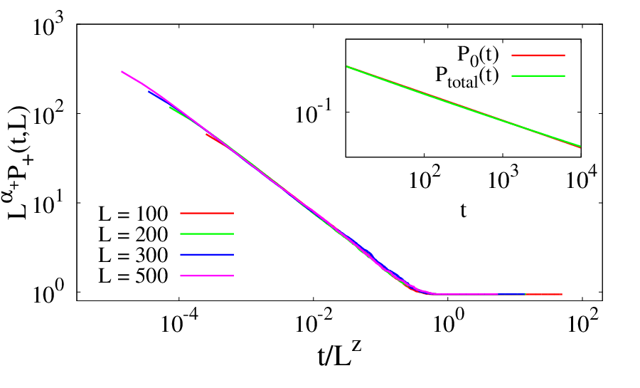
with . We check whether this is also valid when . Obviously, if valid, the associated exponent should vary with , since is constant. Finite size scaling analysis in one dimension was performed for all the three variants of the persistence probability for . Simulations were made for system sizes taking average over at least 1000 configurations. In each Monte Carlo step, spins are chosen randomly and updated. Asynchronous updating rule is used and periodic boundary condition imposed. We find that indeed the finite size scaling (4) is valid, as the curves for different values of collapsed with proper choice of , keeping (Fig. 1). It is checked that these values of are consistent with the relation . In Table 1 we have summarised the values of and obtained for two different values of . The values of and differ from the exact values by less than 0.05%. As for the up, down and total spins is different, the corresponding values , and also turn out to be different.
, the total persistence is expected to be a weighted average of and . We calculate the quantity
| (5) |
to check whether and are equal and find a very good agreement indeed (inset of Fig. 1). Even though (5) is valid, it is interesting to note that the exponent associated with the total persistence probability is different from the , albeit close to it (see Table 1).
| 0.3 | 0.227 | 0.562 | 0.212 | 0.42 | 1.0 | 0.40 |
|---|---|---|---|---|---|---|
| 0.4 | 0.318 | 0.463 | 0.285 | 0.64 | 0.94 | 0.57 |
Qualitatively, the algebraic decay of and can be explained from the behaviour of the exit probability which in the one dimensional Ising model is given by . This indicates that there is a finite probability of ending up with either all up or all down spins even for values of (except for and ).
III Results in two dimensions
In the ordering dynamics of the two dimensional Ising model, the three variants of persistence were studied for various values of less than on square lattices with . Simulations were performed for 1000 configurations. Here also one Monte Carlo time step comprises updates and random asynchronous updating rule is used. Helical boundary condition has been imposed for the simulation in two dimesnions. In Fig. 2, the results for close to 0.5 are shown. As deviates from 0.5, shows a faster decay while both and saturate at higher values. No appreciable finite size dependence is found for these two persitence probablilities (inset of Fig. 2).
By the present convention, is the persistence probability for the down spins, which is the initial majority. Generalising the notation for initial majority and minority spins, we have saturating to a finite value and going to zero. To explain why does not show system size dependence, we can argue like this: had it been decreasing with size, it would ultimately go to zero. On the other hand, had it been increasing for larger sizes, it would approach 1. Both the possibilities are unrealistic and hence no system size dependence is observed. Since is basically a weighted average of and , its nature is dominated by that of , the majority spins, and hence it does not show finite size dependence also.
The persistence probabilities do not show algebraic behaviour unlike in the one dimensional Ising model. The persistence probability for majority spins as well as for the total spins do not show much interesting behaviour as they decay to rather high saturation values and show no finite size dependence. However in case of the minority spins, finite size effect is apparent and a number of interesting features are revealed on further analysis. The decay of the persistence probability can be fitted to the form
| (6) |
which is a combination of an algebraic decay accompanied by an stretched exponential cutoff (Fig. 3). We find that this fit is valid almost up to the time where saturates to a finite value. The fits become more accurate as approaches 0.5. It is clear that extrapolates to a zero value for . However, the versus curves for different values of (shown in the inset of Fig. 3) shows that the finite size dependence is evident only at times beyond which saturates. This is very similar to what happens for . Thus it is sufficient to use eq. (6) for the maximum size () only.
No exact result is known for the persistence exponent even for and one depends only on approximate estimates, most of which are numerical [4, 21, 22, 23]. However, the behavior of the persistence probability has been found to be strictly a power law even for finite system sizes. The resultant exponent has been shown to have some finite time dependence on closer examination [23]. In the present case therefore, we have varied the range of time when eq. (6) is used. Noting there is not much variation in the values of and for different ranges, we have used the average values for further analysis.
In order that the eq. (6) is valid for , must diverge at that limit. Also, the associated exponent should be close to according to the more recent estimates of the persistence exponent in two dimensions. To check this, we analysed the behaviour of and as a function of , where .
The variation of with is found to be of the form
| (7) |
thus showing the divergence at (Fig. 4). The value of is numerically equal to 2.31 . On the other hand, the data for shows some fluctuations but apparently has a linear variation with . In general can be written as , where
| (8) |
Putting , we obtain which is indeed very close to the persistence exponent in two dimensions. . The data is shown in Fig. 4 (inset). The value of is quite insensitive to the value of which may vary between 0.8 to 1.2 due to the scatter in the data. Thus we find the presence of two quantities and which diverge and vanish respectively as . The value of is and it also shows a slow decrease with . However, it remains finite () even at values of very close to 0.5.


The nature of the persistence probabilities in the two dimensional Ising model can also be explained qualitatively by studying the exit probability. It is known that exactly at , the system may not reach the all spins up or down configuration always due to freezing [7, 8, 9]. Since for finite sizes it is possible that such frozen states may persist at small deviation from as well, we considered only those configurations which led to the true ground states while calculating . for the two dimensional Ising model shows strong finite size effect and the data indicate that there is a step function behaviour in the thermodynamic limit. Finite size scaling analysis of was done using the scaling form valid for such a behaviour [24]
| (9) |
where for and for (i.e. a step function like behaviour) shown in Fig. 5. This scaling argument indicates that is basically the factor by which the width of the region, where is not equal to 0 or 1, decreases. The value of from our data collapse is estimated to be . The scaling function is found to fit with the form
| (10) |
with .
Since shows a step function like behaviour in the thermodynamic limit, for an initial concentration of up spins less than 0.5, the probability to reach a configuration with all spins up is simply zero. Hence all the minority spins eventually flip state and therefore .
As already noted, the scaling form (9) suggests scales as and using this in (7) we get where . Hence can be interpreted as a dynamic exponent connecting time and length scales. The only other known dynamic exponent is (eq. 3) associated with the domain growth phenomena and is clearly different from .
IV Summary and discussion
In summary, we obtained the persistence probability of up, down and total spins for Ising spin-systems using the zero temperature Glauber dynamics in both one and two dimensions. In the initial state, the up spin density varies between 0 and 1, while the spins are otherwise uncorrelated. In one dimension, the exact results for the persistence exponents are known and we find that the well known finite size scaling form is valid even in the non-homogeneous case.
In two dimensions, the results differ drastically, no algebraic decay is observed for the three types of persistence probabilities. The persistence probability corresponding to the initial minority spin vanishes. saturates to a finite value consistent with the behaviour of the exit probability. The most significant finding is the diverging time scale associated with the minority spin persistence probability. This timescale is related to the system size through an exponent , not explored so far to the best of our knowledge. In addition we obtain two other exponents and . The values of the exponents obtained in the present study are all close to multiples of 0.5 (within error bars) which suggests that these may be related to the growth exponent . If this can be shown directly it will lead to a very important and striking result that domain growth and persistence probability are no longer independent for . However, this a difficult proposition as exact analytical estimate of persistence has been possible in one dimension only. Hence the existence of yet another independent dynamical exponent in the ordering process in the two dimensional Ising model remains an open question as of now.
Comment: The results presented in this paper have been later improved by generating new data especially closer to x = 0.5. A re-analysis of the scaling collapse leads to the value for . The estimate of using this value is 1.86. Hence it can not be strongly stated that is different from 2.
Acknowledgement: The authors thank CSIR (Sanction No. 03(1287)/13/EMR II) for their financial support. Discussion with S. Biswas and P. Ray are also acknowledged.
References
- [1] A. J. Bray, Adv. Phys., 43, 357 (1994).
- [2] P. L. Krapivsky, S. Redner and Eli Ben-Naim, A Kinetic View of Statistical Physics (Cambridge University Press, Cambridge, 2010).
- [3] B. Derrida, J. Phys. A 28, 1481 (1995); B. Derrida, V. Hakim, and V. Pasquier, Phys. Rev. Lett. 75, 751 (1995).
- [4] A. J. Bray, S. N. Majumdar and G. Schehr, Adv. Phys. 62, 225 (2013).
- [5] A. Lipowski, Physica A, 268, 6 (1999).
- [6] T. Blanchard, M. Picco, Phys. Rev. E 88 032131 (2013).
- [7] V. Spirin, P. L. Krapivsky, and S. Redner, Phys. Rev. E 63, 036118 (2001).
- [8] V. Spirin, P. L. Krapivsky and S. Redner, Phys. Rev. E 65, 016119 (2001).
- [9] J. Olejarz, P. L. Krapivsky, and S. Redner, Phys. Rev. E 83, 030104(R) (2011).
- [10] S. Biswas, A. K. Chandra and P. Sen, Phys. Rev. E 78, 041119 (2008).
- [11] H. Hinrichsen, Adv. Phys. 49, 815 (2000).
- [12] J. Olejarz, P. L. Krapivsky, and S. Redner Phys. Rev. Lett. 109, 195702 (2012).
- [13] K. Barros, P. L. Krapivsky and S. Redner, Phys. Rev. E 80, 040101 (2009).
- [14] J. Ye, J. Machta, C. M. Newman, and D. L. Stein, Phys. Rev. E 88, 040101 (2013).
- [15] S. Chakraborty and S. K. Das, arXiv:1509.07590v1
- [16] C. Godreche and M. Pleimling, arXiv:1505.06587v2
- [17] S. Biswas and P. Sen, Phys. Rev. E 80, 027101 (2009)
- [18] G. Manoj and P. Ray, Phys. Rev. E 62, 7755 (2000).
- [19] S. Jain and H. Flynn, J. Phys. A: Math. Gen. 33 8383 (2000)
- [20] E. Ben-Naim, L. Frachebourg and P. L. Krapivsky, Phys. Rev. E 53, 3078 (1996).
- [21] B. Yurke, A. N. Pargellis, S. N. Majumdar and C. Sire, Phys. Rev. E 56, R40 (1997).
- [22] S. N. Majumdar and C. Sire, Phys. Rev. Lett. 77 1420 (1996).
- [23] T. Blanchard, L. F. Cugliandolo and M. Picco, J. Stat. Mech. 2014 12021 (2014).
- [24] S. Biswas, S. Sinha and P. Sen, Phys. Rev. E 88, 022152 (2013).
- [25] P. Roy, S. Biswas and P. Sen, J. Phys. A: Math. Theor. 47 495001 (2014)