Explaining quantum correlations through evolution of causal models
Abstract
We propose a framework for the systematic and quantitative generalization of Bell’s theorem using causal networks. We first consider the multi-objective optimization problem of matching observed data while minimizing the causal effect of nonlocal variables and prove an inequality for the optimal region that both strengthens and generalizes Bell’s theorem. To solve the optimization problem (rather than simply bound it), we develop a novel genetic algorithm treating as individuals causal networks. By applying our algorithm to a photonic Bell experiment, we demonstrate the trade-off between the quantitative relaxation of one or more local causality assumptions and the ability of data to match quantum correlations.
While it seems conceptually obvious that causality lies at the heart of physics, its exact nature has been the subject of constant debate. The fundamental implications of quantum theory shed new light on this debate. It is thought these implications may lead to new insights into the foundations of quantum theory, and possibly even quantum theories of gravity [1, 2, 3, 4, 5, 6, 7, 8, 9, 10].
These realizations have their roots in the Einstein-Podolski-Rosen thought experiment [11] and the fundamental theorems of Bell [12] and of Kochen and Specker [13]. A cornerstone of modern physics, Bell’s theorem, rigorously excludes classical concepts of causality. Roughly speaking Bell’s theorem states that the following concepts are mutually inconsistent: (1) reality; (2) locality; (3) measurement independence; and (4) quantum mechanics.
In philosophical discussions, typically one rejects (1) or (2), which together are often referred to as local causality, though the other options have been considered as well. In studies with an operational bent, however, one often considers relaxations of (2) or (3) which is what we concern ourselves with here. These relaxations have been addressed from different perspectives, but only regarding specific causal influences in isolation [14, 15, 16, 17, 18, 19, 20, 21, 22, 23], whereas here we wish to study all possible relaxations of the causal assumptions implied by (2) and (3) simultaneously.
The framework of causal networks [24, 25] is wildly successful within the field of machine learning and has led some physicists to utilize them to elucidate the tension between causality and Bell’s theorem. Recently, Wood and Spekkens have shown that existing principles behind causal discovery algorithms (namely, the absence of fine tuning) still cannot be reconciled with entanglement induced quantum correlations even if one admits nonlocal models [9]. However, such results only hold for the exact distributions, and would not necessarily apply to experimental data due to measurement noise, or a relaxation of the demand of reproducing exactly the quantum correlations. Clearly, the further away from the quantum correlations one is allowed to stray, the more likely a locally causal model can be found.
Here we propose a framework for systematic and quantitative generalizations of Bell’s theorem by using causal networks. The idea, depicted in Figure 1, is to consider the multi-objective optimization problem of matching the observed data from an experiment while minimizing the causal effect of nonlocal variables. It is in this sense of matching experimental data that we are explaining the quantum correlations. Our first contribution is a rigorous lower bound for this optimization problem, demonstrating a generalization of Bell’s theorem. Theorem 1 below establishes that there must exist a tradeoff between the goodness of fit to experimental data and the quantitative amount of causal influence for any model.
This theorem rules out a portion of the space allowed by this new framework, but the bounds are not tight. To solve the optimization problem, and hence numerically find the optimal bounds, we develop a type of genetic algorithm called a multi-objective evolutionary algorithm (MOEA) to quantify the relaxations necessary to reproduce the data generated by experiments on entangled quantum systems [26, 27, 28]. Our genetic algorithm treats as individuals causal networks and we develop genetic operators which represent the evolution of these networks. By applying our algorithm to a photonic Bell experiment, we show that the tradeoff between the quantitative relaxation of one or more local causality assumptions and the ability to match quantum correlations appears linear.
The outline of the paper is as follows. In Section I and Section II we set out the background of the causal models we use and the mathematics required to convert a probability distribution into a fitness function. In Section III we provide analytic bounds on causal influence. In Section IV we describe the experiment that provided the input to the algorithm. Section V briefly describes the result of applying the genetic algorithm to the experimental data. Section VI describes the process by which we convert the problem into one that can be explored using evolutionary operators and details the construction of the algorithm. We conclude in Section VII with a discussion.
I Causal models for Bell Experiments
The formalism of causal models allows us to quantify the relaxations necessary to avoid the contradiction in Bell’s theorem and, more importantly, explore the trade-offs necessary in minimizing the amount by which the assumptions are violated. Building off the work of Chaves et al [29], we make all this concrete through a quantification of the relaxation of each assumption in the context of causal models. The task of minimizing the amount of the relaxation is a multi-objective optimization problem. Bell’s theorem is recast as the statement that all objectives cannot be simultaneously minimized. We explore the trade-offs through the concept of Pareto optimality.
The prototypical “Bell experiment” has two distant parties, often named Alice and Bob. We suppose that Alice and Bob each have devices with binary measurement settings, respectively labeled and . Conditioned on these measurement settings, their devices also record binary events, labeled (Alice) and (Bob). Suppose it is empirically observed that and are correlated. Bell defined a locally causal model of such correlations as follows: there exists a “hidden variable” which is the common cause both of conditioned on , and of conditioned on . We write these random variables as and , respectively. Formally, the general conditional distribution is assumed to satisfy
| (1) |
Moreover, it is assumed that the choices of settings can be made such that each of and can be set independently of the hidden variable ,
| (2) |
Such an assumption is often motivated by the injection of randomness into the measurement settings or the free-will of Alice and Bob. Bell’s theorem can be stated succinctly as follows: the conditional distributions describing the outcomes of some experiments on quantum systems cannot be factorized as in Eqs. (1) and (2).
A causal network is a directed acyclic graph with nodes representing random variables and edges denoting causal relationships between variables. The defining feature of such networks is the factorization of joint probabilities. Generally, suppose we have nodes , each of which represents a random variable in our model. We will assume that each such random variable is discrete, and without loss of generality, will assume integer labels for its possible values. The edges in the causal network of these variables are defined such that
| (3) |
where denotes the parents of node .
Take, for example, the causal network in Figure 2a. In general, we can decompose the joint distribution in terms of conditional distributions as
| (4) |
Using the causal network to eliminate conditionals, (3) implies
| (5) |
which are identical to Bell’s assumptions on local hidden variable models. Thus, Bell’s theorem is equivalent to the statement that certain quantum correlations cannot be realized by the causal network in Figure 2a.
II Relaxing Bell’s assumptions
It is known that quantum mechanical correlation arising in a Bell-type experiment can however be explained by adding a new causal link to the local hidden variable network [15, 18]. Two examples are shown in Figure 2. In many practical cases, these causal links are not entirely unphysical from the standpoint of respecting relativity and free-will, for example. The reason being that experiments do not actually conform to the exact assumptions Bell made—there are noisy detectors, non-random number generation, losses, inability to space-like separate “Alice” and “Bob,” and so on. When this is the case, such causal models are said to be exploiting loopholes.
In Figure 2b, a causal model that allows correlations between the measurement settings is shown. In the same spirit, we could have had either or be causally dependent on or another hidden variable. Such models are often called superdeterministic and are ruled out by the assumption that Alice and Bob are not colluding and have free-will or access to independent randomness. If the experiment only approximately satisfies these assumptions—perhaps due to low detection efficiency—one can still model the data with a local hidden variable said to be exploiting the detection loophole [30]. The question of quantifying the amount of independence of the measurement settings necessary has been addressed from multiple perspectives and has practical quantum cryptographic consequences [15, 16, 17, 18, 19, 20, 21, 22].
In Figure 2c, a causal model which allows correlations between the measurement outcomes is shown. This is, and similar models are, called nonlocal and could potentially even allow for superluminal signaling. A quintessential example of a nonlocal model which reproduces the predictions of quantum theory is Bohmian mechanics. Toner and Bacon studied the amount of nonlocality necessary to simulate quantum correlation in the context of classical communication costs [14, 23], while Wolf has expressed nonlocality in terms of the compressibility of experimental observations [31].
The current studies, mentioned above, quantifying the relaxations of the causal assumption necessary to replicate quantum correlations are rather disjoint. Recently, Chaves et al. placed the question in context of causal networks and found that some measures of these relaxations can be cast as efficiently solvable linear programs [29]. We build on this idea and consider a completely abstract framework amenable to any set of random variables using a single measure of the causal influence of one variable on another. This allows us to consider all possible relaxations simultaneously and thus explore the trade-offs necessary to simulate quantum correlations with hidden variable models.
We will now state our model more technically. For consistency we formulate the problem in the context of the two-party Bell experiment, but we emphasize that this approach generalizes in an obvious way to any set of random variables. A model, , is specified by a joint distribution
| (6) |
We label the empirical frequencies and denote the total variational distance (TVD) of a model to these frequencies by
| (7) |
where the vector being normed is labeled by . Here the 1-norm of a vector is simply .
The causal influence is defined for a general graph as follows:
| (8) |
where is the set of parents of that are not also grandparents of , and where indicates that the maximization over , and is restricted to feasible assignments. That is, the maximization does not consider assignments outside the support of . In words, the causal influence is non-zero when changing leads to a change in . It is quantified by maximizing over latent variables of the target that are not also latent variables of the control.
For example, if we want to minimize the causal influence between two variables to in Figure 2c we consider
| (9) |
We include the conditions to prevent the causal influence being maximized by an assignment outside the support of the random variable ; the maximization should be taken over all feasible assignments.
Intuitively, this definition represents how distinguishable the different settings of are when viewed through measurements of . That is, if does not causally affect , then it is not possible for a change in to be detectable through alone. We adopt this definition in lieu of the traditional approach of using interventions, wherein an external agent imposes a particular value of while holding all else fixed, effectively cutting out any causal links incident on other than one originating from the experimentalist themselves. Though some novel experiments have been performed using intervention to reason about quantum mechanics [32], we cannot intervene on quantum mechanical models in general, such that we must instead maximize over conditions for the experiment, here represented by the maximization over and .
The task then is to find a model which minimizes TVD and for each ruled out by local causality and measurement independence. If the empirical frequencies contain some causal dependence between two variables, then either the model must also contain such causal dependence or the observed frequencies from the model must be different from the empirical frequencies. Perhaps interestingly, one might be able to “trade” unwanted causal influence between one pair of variables for another, while maintaining the same TVD. Thus, the problem of determining “how much” relaxation of Bell’s causal assumptions is necessary to match an empirical observed frequency becomes much more interesting and nuanced.
Suppose two models and both match the data equally well—i.e. — but has some unwanted casual influence , say, and does not—that is, . Clearly, is preferred and we say is dominated by . For many objectives, the situation is more complex but can be handled by the concept of Pareto optimality.
Let be the set of all models. Let each model’s fitness be represented by the function , where is number of objectives. Define the partial order as follows:
| (10) |
for all . If , we say dominates (or is equivalent to , if holds as well). The set of Pareto optimal models is now defined as follows:
| (11) |
This says that a model is Pareto optimal if the set of other models which dominate it is empty. In other words, the Pareto optimal is the set of non-dominated models.
III Analytical bounds
In this section, we provide analytical bounds which relate the amount of causal influences exhibited by any model to its agreement with the empirical frequencies . For the sake of simplicity, we restrict ourselves to analyzing the causal influence between the variables and —see Figure 2c. However, we emphasize that analogous statements are valid for causal influences between any two variables. For the variables and , the empirical frequencies themselves admit a causal influence
| (12) |
which is defined in complete analogy to (9). To state our theorem, we must define two more quantities. Let be the set of models having with respect to the empirical frequencies , and denote by the minimum empirical marginal frequency.
Theorem 1.
For all models and ,
| (13) |
We point out that the bound (13) becomes loose and eventually diverges if the minimum empirical marginal frequency approaches zero or if the of the class of models becomes too large relative to .
The proof of Theorem 1 can be found in Appendix A.
IV Bell experiment and data
As input for the MOEA we use data from a polarization photonic Bell experiment, shown in Figure 3 [33]. Indistinguishable horizontally polarized () photon pairs are generated via type-1 spontaneous parametric down-conversion. Both polarization qubits are rotated into a diagonal state by a half wave plate (HWP) with fast axis at from vertical, where denotes vertical polarization. A polarization phase rotation is applied to photon 1 by two quarter wave plates (QWPs) and a HWP, while photon 2 has its state optimized by a polarizing beamsplitter (PBS). Both photons are collected in polarization maintaining optical fiber (PMF) and are incident on the two input faces of a fibre-coupled PBS, which transmits and reflects , preparing Alice’s and Bob’s qubits. The configuration of the optical fibres results in a operation applied to Alice’s qubit. By measuring in the coincidence basis, we post-select the state
| (14) |
where are the Bell states with subscript () corresponding to Alice’s (Bob’s) qubit. The parameter defines the coherence of the state which depends on the overlap of the two photons after the fibre-coupled PBS and is controlled by the optical delay line (ODL). The state prepared when is a maximally entangled Bell state and when is an incoherent mixture . The polarization tomography setup in Figure 3 enables projection onto any pure state and can be used for two-qubit state tomography [34]. The photons are detected with silicon avalanche photo-diodes and coincidence counts recorded by a timing card.
Our input for the MOEA is a normalized frequency distribution across binary measurement settings for Alice () and Bob (), and binary measurement outcomes and respectively. The measurement settings are controlled by wave plate angles in the tomography and the measurement outcome is the collapse of the state onto one of the four basis state , , or . A single measurement is the number of photon pairs recorded for a fixed integration time and can be written as for measurement settings and measurement outcomes . is the total photon flux, is the integration time and is the operation of the wave plates. We calculate by measuring all combinations of , , and , and normalizing by the total number of photon pairs recorded. We note that this experiment is not performed in a loophole-free way, but nonetheless provides us with the quantum correlations we wish to analyse.
Typically, Bell experiments aim to violate the CHSH inequality [35], confirming that quantum mechanical systems cannot be described with local hidden variable models. The CHSH inequality is calculated as
| (15a) | ||||
| (15b) | ||||
where defines the correlation between Alice’s () and Bob’s () measurements, given as
| (16) |
While the CHSH inequality holds for systems which respect local causality, a pair of quantum entangled particles can achieve a maximum value of . By tuning the parameter in (14), then for measurement settings fixed to be optimal for the case , we can prepare states that obey the CHSH inequality when and states that violate it. In order to achieve the maximum violation of the CHSH inequality, it is necessary to chose specific wave plate angles for and . Here, we are not interested in violating the CHSH inequality; however, we can use it to benchmark our results from the MOEA.
V Edge of reality

Using the experimental data (where ), we searched for the Pareto optimal models by developing a multi-objective evolutionary algorithm to find the best underlying probability distributions for a causal network. Since this represents a trade-off between a local realistic model and real-world correlations, we call the Pareto optimal surface the “edge” of reality.
An individual of the population is a probability distribution over the nodes of a given causal network (each such individual is a causal model, ) and its multi-objective fitness depends on how close the model can reproduce the experimental data and the amount of causal influences between nonlocally separated variables.
As an initial step, we examined relaxing one casual edge at a time, beginning with a causal influence from to —that is, Alice’s outcome is allowed to influence Bob’s. The Pareto front (the numerical approximation to the Pareto optimal) is shown below in Figure 5. Like the theoretical bounds (which while not linear, are nearly so in the considered domain), the front appears to be linear (Pearson’s value of 0.997, with bisquare robust fitting). That is, increasing locality violations allows observed (quantum) correlations to be more exactly matched, the trade-off being approximately linear in nature. Next, we relax the causal edges and simultaneously. The found Pareto front is shown in Figure 6. Again, we see that the front appears linear (). We have also used our algorithm to test other causal networks and found the results to be quantitatively identical to these two cases.
VI The Evolutionary Algorithm
In order to find the Pareto front of solutions, it is necessary to find feasible probability distributions that give rise to the required TVD with the required causal-violations(s). There is no known way of doing this analytically. Even in simple single edge causal models the search space is prohibitively large and objective non-convex. This search space grows rapidly with additional causal edges. Evolutionary Algorithms are known methods for finding such Pareto fronts where there is only limited knowledge of the underlying search landscape. We wish to numerically find the Pareto optimal set of models representing Bell experiment data. To do so, we use evolutionary computation [36].
Such algorithms are generally well studied for functions of the form . However, here the domain of our objective function is , i.e. the probability distributions on the causal network. Consequently, there are implicit constraints on the relative values these distribution can take (for instance, in each node they need to sum to 1) and so we have devised a set of evolutionary operators that allow the probability distribution of an arbitrary causal network to be evolved. With this we combine several evolutionary computation strategies to evolve and explore the Pareto front of a given arbitrary network.
VI.1 Evolutionary Algorithm Overview
As the cornerstone of our multiobjective evolutionary algorithm (MOEA) we utilize the well-known and well-understood NSGA-II algorithm [39]. Although the NSGA-II algorithm specifies both the generation and selection procedures, we utilize the the DEAP software library [37] which provides the NSGA-II algorithm only for the “select” stage. The method by which we proceed is to use the algorithm (detailed in Algorithm 1) where we set to be the population size. For the purposes of avoiding confusion we note that the is more properly an algorithm used with a subset of evolutionary algorithms known as evolutionary strategies, and thus is not part of the toolkit of the seperate branch known as genetic algorithms. Consequently, our algorithm is not strictly a genetic algorithm but is an evolutionary algorithm. Although we use an implementation of , by setting the algorithm is functionally equivalent to the generation algorithms used in genetic algorithms. In this paper we make no distinction between genetic algorithms and the more general term evolutionary algorithm in the classification of the algorithms used. The overall implementation of the algorithm is thus functionally identical to the original NSGA-II algorithm, save that the selection of parents is random rather than by binary tournament selection.
Consequently this evolutionary algorithm proceeds in generations, each of which consists of producing offspring from the previous generation’s population, then selecting individuals from the combination of the previous population and the new offspring to form the new population. As detailed in Algorithm 1 the algorithm is expressed abstractly in terms of genetic operators that create, crossover, evaluate and select individuals within each population. Thus, we form our algorithm by specifying what an individual is, the fitness functions that we use in evaluating individuals, and by providing suitable genetic operators to create “children” causal networks.
VI.2 Representation of Individuals
Effectively, our genetic algorithm searches for Pareto optimal models by representing as an assignment of conditional distributions to each node in a causal network with a fixed structure. Since the random variables at each node are constrained to be discrete, we represent the conditional distributions by tensors, such that finding arbitrary joint, marginal and conditional distributions over subsets of the nodes is then an exercise in standard tensor contractions.
In particular, consider a node with causal parents . Then, the distribution is given by the tensor
| (17) |
where we have used square brackets to indicate indices (similar to C- or Python-style notation).
We can contract repeated indices of two such tensors with the tensor at a corresponding third node to perform expectation values. For example, let be the tensor for , be the tensor for and be the tensor for in the model of Figure 2c. Then, to find , we compute
| (18) |
The general case, allowing for arbitrary numbers of random variables and conditions, is given as Algorithm 2.
VI.3 Fitness Functions
Our algorithm uses two different kinds of fitness functions:
- 1.
The total variational distance (TVD) between the joint distribution computed from an individual and the observed frequencies.
- 2.
Causal inflences along penalized edges, as generalized from the definition given by (9) in Section II.
Dealing with each in turn, the TVD is calculated by taking the vector 1-norm between the flattened joint distribution tensor the observable variables calculated as in subsection VI.2 and the flattened observed frequencies,
| (19) |
where is an individual with joint distribution tensor over all observables, is the tensor of observed frequencies, and where indicates flattening— that is, reduction of an arbitrary-rank tensor to a rank-1 tensor.
As discussed in Section II, we adopt a definition of causal influence that allows us to reason even in lieu of interventions. Our definition of the causal influence for an individual proceeds in three steps. First, we maximize over pairs of settings of to find which are most distinguishable through observations of alone. We then maximize over the conditions under which these observations are made, represented by maximizing over feasible assignments to the parents of . Finally, we marginalize over those nodes which are also parents of to prevent “hiding” causal influence; this is illustrated in Figure 7.
VI.4 Genetic Operators
Having defined the mapping from models to individuals, we complete the specification of our algorithm by detailing the various genetic operators which act on these individuals.
Creation
In order to create a new individual , we must specify
a new conditional distribution at each node of the causal graph. We do so
randomly by assigning a tensor with entries drawn uniformly from
to each node, then renormalizing to ensure
.
Using the tensor notation defined above,
| (20) |
where is the unnormalized tensor of at .
Crossover/Mating
Given two individuals and , we mate them to produce two new individuals and by swapping the tensors at each node with probability . That is, for each node , the corresponding tensor of is given by
| (21) |
Mutation
Given a single individual that has been selected for mutation, we proceed by first picking a node on the causal graph uniformly at random, with corresponding tensor (assuming parents) .
One of the conditional events represented by (that is, a single element of the tensor) is selected at random and the value (and hence the probability assigned to the selected outcome) is randomly increased or decreased by a sample from a zero-mean Gaussian distribution, where the variance is a user supplied parameter. The mutated element of is then clipped to the interval , and the relevant tensor index renormalized such that (20) holds.
By way of example, if we had a node with binary values, which in turn had one parent also with binary values, then the information pertaining to that node would be stored in a tensor corresponding to the probability distribution
where represents the probability of being 0 given is 0 and so on. From this it can be seen that it is necessary that . One of , , or would be modified as discussed above, and the remaining values renormalized to ensure that the relevant probabilities continue to sum to 1.
Selection
For selection we used an unmodified version of the NSGA-II algorithm [39]. NSGA-II uses a fast sort algorithm to locate the non-dominated individuals and then applies a crowding distance sorting algorithm to prefer those individuals that explore different parts of the pareto front. The “best” individuals are retained for the next generation.
VI.5 Decomposition of the multi-objective optimization (the Island Model)

Here we present an enhancement to the basic genetic algorithm discussed above that aids the discovery of the global Pareto front in multi-dimensional scenarios, where—as is the case here—it is possible to evolve populations to occupy the extremes of any particular front.
As discussed in subsection VI.7 it is well known that the NSGA-II crowding becomes less effective with the exponential increase in the size of the front with the number of dimensions. However, in our case are we able to force the population to start at extreme points of the Pareto front by pre-evolving the population on structurally reduced graphs or with reduced fitness criteria. These populations are able to seed the graph we wish to explore and spread over the front, fleshing it out over multiple runs. This can then be repeated as we increase the dimensions of the fronts. This is not dissimilar to the mechanism used in NeuroEvolution of Augmenting Topologies (NEAT) [40] where populations are evolved on small neural networks prior to allowing additional links to be added. A similar idea of decomposing the objectives is explored in [41]. Effectively, where a multiple dimension Pareto front needs to be explored, different populations are evolved on all permutations of the simpler graphs (on seperate “islands”) before being brought together for evolution over the full graph. This is illustrated in Figure 8.
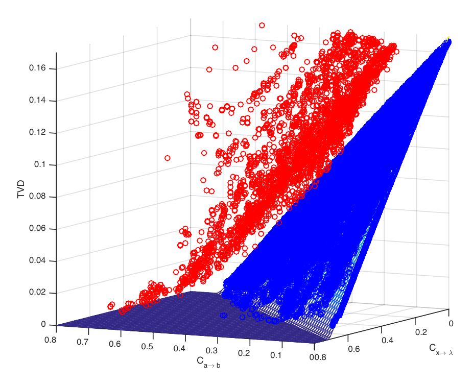
This technique allows us to find a three-dimensional Pareto front based on a graph with two causal edges, from as well as . This was evolved using five runs of the “island model” detailed above. For each run the initial islands had a population of 300 and comprised 4 runs of 400 generations. The initial runs found populations clustered around the three extremes: (1) min(TVD), hold , ; (2) min(), hold TVD , ; and (3) min(, hold TVD , .
The second set of islands take the relevant individuals generated above, reduce them to the best 400 individuals representing the extreme of the Pareto fronts for that island and transplant them to expanded causal network graphs. In this case there are two second generation islands: one generating the two-dimensional Pareto front for {TVD and }, with held to be 0 (i.e. no causal link); and the second the two-dimensional Pareto front {TVD and }, with held to be 0. These populations are then evolved on the respective causal networks generating two dimensional Pareto Fronts similar to Figure 10. These populations are placed in an -Dominance archive. (In other-words they are only kept if they dominate all previous individuals by at least , where in this implementation was ). The entire process so far is repeated several times (in this experiment 5 times) to ensure we have 2,000 suitable individuals in the archive. These individuals are, effectively, clustered on the two dimensional fronts specified in the second set of islands. This final population is used to generate the 3-dimensional Pareto front shown in Figure 9. The final island had a population of 2,000 individuals (extracted initially from the -Dominance archive), evolved for 800 generations. This constituted one run of the island model. The Model was run 5 times, with every individual generated by the model being submitted to (but not necessarily accepted by) the global -Dominance archive.
To illustrate the advantage of using this model, we have also plotted (in red) the best Pareto front found using just the basic algorithm (i.e. evolving only over the full graph). These additional points were collected over 8 runs, using a high population (6,000) and represented five times the computing power required for the Island Model. As can be seen the global -Dominance archive for the basic algorithm contained few individuals on the best global Pareto front found by the Island Model. The Pareto front for the Island Model (plotted blue) does appear to be a viable candidate for the actual global front, indicating that - for this model - the trade-offs in the different causality violations considered is linear. The front fits a linear plane with a Pearson’s value of 0.9902, the non-fitting points being those with extremely low TVD values (the points which appear on the horizontal part of the mesh). While this still needs to be investigated further we believe it is related to experimental noise which might require increased causal violation to match the noisy data exactly. So far as we are aware this is the first evidence that tradeoffs in multiple causal violations are also linear for such graphs.
VI.6 Previous Work and Design Decisions
Although there has been previous work in using genetic algorithms to explore Bayesian causal networks (e.g. [42], [43] and [44]), the focus of such works has been to create the network and the links therein. For instance, [45] uses a multi-objective genetic algorithm (MOGA) to evolve dynamic Bayesian networks. There the multi-objectives explored were the ability of the evolved networks to explain the data, compared with the complexity of the network in question. The MOGA was used instead of, for instance, a minimum description length (MDL) constraint. In all of these cases the network is being used to model something of interest and then, given some observed values, infer the likely causes. The genetic algorithms are used to construct different models which are then trained, typically the success (or otherwise) of a particular model being its performance on withheld data.
Our work differs because of the way we wish to utilize the Bayesian causal networks, specifically we specify the networks we are interested in, namely those which model a physical view of “reality” with specified local causality violation. Training such networks to replicate observed correlations is of limited interest because successful training results in one specific probability distribution that explains the data. What we are interested in finding are all the relevant probability distributions where the ability to match the observed correlations is contrasted with the strength of the local causality violations. The evolutionary algorithm is used, not to evolve networks, but rather to find these probability distributions given the network. The MOEA is used to guide evolution along these Pareto fronts.
In order to explore the Pareto front some type of MOEA algorithm is required. MOEA on two or three dimensions are relatively well understood. Algorithms to explore large dimensions are still an active area of research (see for example [46]). Since our initial experiments (reported here) would only require causal networks with no penalized edges (a single-value optimization), one penalized edge (a MOEA with a two-dimensional Pareto front) or two penalized edges (a MOEA with a three-dimensional Pareto front), we decided to use the well understood NSGA-II [39]. Although NSGA-II attempts to return the whole of the Pareto front in a single run it was quite clear that the search space (being the required probability assignments for all the nodes in the network) was not smooth, even though the Pareto fronts may be (and, in fact, turned out to be) smooth. Given this an -Dominance Archive [47] was maintained and updated through multiple runs. In order to maintain diversity between runs the archive was not used to guide the evolution, but rather served as an updated archive of the best Pareto front found so far. After completing multiple runs, the individuals in the archive thus represent the Pareto front for the entire procedure, rather than for each run taken in isolation.
In subsection VI.5 we describe how the -Dominance Archive generated from a lower dimension front can be used to seed evolution when a higher dimensional Pareto front is explored, in a manner not dissimilar to the algorithm presented by Liu et al. [41] or utilized by Stanley and Miikkulainen [40].
VI.7 Implementation methodology and details
Our initial runs with the EA (i.e. the MOEA with a single objective, being to minimize the TVD) were used to verify that the EA could match known results. In this case we start with a causal network that reflects Bell’s non-locality assumptions (as shown in Figure 2a) and for various values of in (14) use the EA to try and match the experimentally observed joint probability distribution. This is a single-objective EA, with fitness being governed solely by the TVD, i.e. by how closely the observed probability distribution of the Model (being the observed joint probability distribution for an individual over the local causal graphs) matches the experimental data. It is known that when is less than the observed data can be modeled with a local causal network. The TVD values should increase as increases to 1 since the empirical distribution no longer factorizes into a locally causal distribution.
An initial population of 300 () was chosen, with the probability of crossover, being 0.1 (and mutation 0.9). The mutation operator used a standard deviation of 0.1 (see subsection VI.4). As is typical for experiments using genetic algorithms no systematic attempt was made to find the “best” parameters for the algorithm. Rather during the course of some initial testing runs, runs with variations of parameters were tried and the parameters of the ones that seemed to find solutions quickest were used. Population sizes reflected those minimum populations required to avoid runs being trapped early on in local minima. The parameters reported are not reported in a claim of optimality, but rather are reported for the purposes of reproducibility. In any case, once a solution is obtained, its validity does not depend on the means by which it was found.
Figure 4a shows experimentally measured density matrices for a range of state values. The reduction in coherence is observed as decreasing off-diagonal terms. Figure 4b shows the minimum TVD values emerging from 20 runs of the graph for various values together with a linear line fitting the data, running from the known y-intercept of 0 TVD for . As can be seen the EA fits the expected linear results (Pearson’s ).
Having ensured that the algorithm could correctly match the known results on a causal network consistent with Bell’s non-locality assumptions, the next stage is to require a relaxation of local causality to allow the EA (now operating as a MOEA) to match the correlations present in entangled states. As an initial step, we examined relaxing one casual edge at a time, beginning with a causal influence from to —that is, Alice’s outcome is allowed to influence Bob’s. This is illustrated in Figure 2c. This becomes a multi-objective problem with a two-dimensional Pareto front, ostensibly well within the capabilities of NSGA-II. The tensor contractions required are not overly complex but with increasing numbers of hidden variables (as a result of additional causal links) each run takes a non-trivial amount of time. As is typical where the search landscape (being the underlying conditional probability distributions) is not smooth (even though the fitnesses such distributions reduce to are smooth) a number of runs failed to converge to any part of the Pareto front, with most runs finding part, but not all of the Pareto front. In Figure 10a we show the individual results of 40 such runs. As can be seen from the figure just under half of the 40 runs had a large percentage of their front non-opitmal, with approximately half the runs being plotted on top of each other on the Pareto Front. To generate the final Pareto front each of the individuals in the -Dominance archive from each of the 40 runs are submitted to the global -Dominance archive, so that the best estimate of the true Pareto front can emerge, as shown in Figure 10b.
Two points arise from these results. The first is that the front appears to be linear, that is increasing locality violations allows observed (quantum) correlations to be more exactly matched, the tradeoff being linear in nature. As far as we are aware this was not previously known. The second arises from the number of failed or only partially successful runs. In particular we note that while in the majority of runs the MOEA was able to find many points on (or close to) the Pareto front, other runs could be trapped and all runs had difficulty at either extreme of the front. It is clear that the search landscape in general is not smooth - the interplay between the conditioning on the hidden local variable and the other probability distributions allow the MOEA to become trapped in some local minima. The larger front (in this case a two-dimensional line) allowed the population to “slide” away from the edge cases. In addition as observed in [9] it is likely the edge cases represent very specific distributions. Whilst some of these observed difficulties could, in part, be ameliorated by using a larger population and relying on the NSGA-II crowding mechanism to prevent such slippage, as is known this will not be feasible if the front consists of three (or more) dimensions. The front grows exponentially with the number of dimensions, requiring an exponential increase in population size. An alternative MOEA such as NSGA-III may help but each alternative comes with their own difficulties and assumptions. It is, however, possible to use the specifics of the problem space to address these concerns. We know we can evolve the population on a more limited graph (such as the purely local graph) and force the population to find the lowest TVD with a causal violation of zero (i.e. in the local graph ). This evolved population can then be “transplanted” on to a graph that does have an link (e.g. Figure 2c). The other extreme (i.e. lowest violation for TVD) can be found with a small alteration to the fitness function. To find this point we evolve the population on the graph representing Figure 2c but with a single-objective fitness function, implemented as minimizing the TVD, but where two individuals have the same TVD, the one with the lowest causality violation is preferred. This drives the population towards zero TVD and then minimizes the causality. Even with this the observed correlations were unable to achieve an exact , it is speculated this is a result of experimental noise. The ability to generate populations (distributions) that sat at the extreme points of the Pareto front allowed the entire two-dimensional front to be revealed and, as discussed below, can similarly be utilized to reveal the three-dimensional front created by two simultaneously relaxed local causality constraints.

VII Discussion
In this work, we have developed a method to allow the study of several relaxations of local hidden variables models simultaneously in a single framework using the tools of casual networks and genetic algorithms.
With further refinement, we hope that our approach can shed light on other scenarios where quantum correlations display richer structure than classical systems would allow. For example, generalizations of the standard Bell scenario to more stations [48, 49] and more outcomes [50, 51], as well as multiple hidden variables [52, 3, 53]. In the latter scenario, very little is known since classical correlations are no longer given by linear constraints. Very recently, Chaves has used the framework of causal networks to systematically study such higher-order constraints [54]. Such measured quantities will be particularly useful to our approach as they can be seen as highly relevant coarse grainings of the exponentially growing data space. Such dimension reduction techniques will be crucial for scaling up our numerical algorithm to the analysis of multi-party quantum correlations.
In addition, there is nothing specifically “quantum” about our core numerical methods. Thus, our approach should find application outside of the problem of understanding quantum correlations. Recently Lee and Spekkens have also used inspiration from the causal analysis of quantum correlations to develop new causal discovery protocols [55]. Like Lee and Spekkens, we depart from the usual considerations of observed correlation to considering the entire joint probability distribution. Our goals differ, however; whereas the aim of Lee and Spekkens is to find all casual models consistent with data, our goal is to find non-dominated models of the plausible correlations. These two approaches are likely to find a harmonious union in the future.
Acknowledgements.
We thank Martin Ringbauer and Andrew White for discussions. This work was supported by the US Army Research Office grant numbers W911NF-14-1-0098 and W911NF-14-1-0103, and by the Australian Research Council Centre of Excellence for Engineered Quantum Systems CE110001013. STF acknowledges support from an Australian Research Council Future Fellowship FT130101744. AP acknowledges an Australian Research Council Discovery Early Career Researcher Award, Project No. DE140101700 and an RMIT University Vice-Chancellor’s Senior Research Fellowship. RK acknowledges additional support from the Excellence Initiative of the German Federal and State Governments (Grants ZUK 43 & 81) and the DFG.References
- [1] M. S. Leifer, “Conditional density operators and the subjectivity of quantum operations,” in AIP Conference Proceedings, Vol. 889 (AIP Publishing, 2007) pp. 172–186.
- [2] M. S. Leifer and D. Poulin, “Quantum graphical models and belief propagation,” Annals of Physics 323, 1899 (2008).
- [3] T. Fritz, “Beyond Bell’s theorem: correlation scenarios,” New Journal of Physics 14, 103001 (2012).
- [4] J. Fitzsimons, J. Jones, and V. Vedral, “Quantum correlations which imply causation,” arXiv:1302.2731 (2013).
- [5] M. S. Leifer and R. W. Spekkens, “Towards a formulation of quantum theory as a causally neutral theory of Bayesian inference,” Physical Review A 88, 052130 (2013).
- [6] M. S. Leifer and R. W. Spekkens, “A Bayesian approach to compatibility, improvement, and pooling of quantum states,” Journal of Physics A: Mathematical and Theoretical 47, 275301 (2014).
- [7] Č. Brukner, “Quantum causality,” Nature Physics 10, 259 (2014).
- [8] E. G. Cavalcanti and R. Lal, “On modifications of Reichenbach’s principle of common cause in light of Bell’s theorem,” Journal of Physics A: Mathematical and Theoretical 47, 424018 (2014).
- [9] C. J. Wood and R. W. Spekkens, “The lesson of causal discovery algorithms for quantum correlations: causal explanations of Bell-inequality violations require fine-tuning,” New Journal of Physics 17, 033002 (2015).
- [10] K. Ried, M. Agnew, L. Vermeyden, D. Janzing, R. W. Spekkens, and K. J. Resch, “A quantum advantage for inferring causal structure,” Nature Physics 11, 414 (2015).
- [11] A. Einstein, B. Podolsky, and N. Rosen, “Can quantum-mechanical description of physical reality be considered complete?” Physical Review 47, 777 (1935).
- [12] J. S. Bell, “On the Einstein Podolsky Rosen paradox,” Physics 1, 195 (1964).
- [13] S. Kochen and E. Specker, “The problem of hidden variables in quantum mechanics,” Indiana Univ. Math. J. 17, 59 (1968).
- [14] B. F. Toner and D. Bacon, “Communication cost of simulating Bell correlations,” Physical Review Letters 91, 187904 (2003).
- [15] J. Barrett and N. Gisin, “How much measurement independence is needed to demonstrate nonlocality?” Physical Review Letters 106, 100406 (2011).
- [16] M. J. W. Hall, “Complementary contributions of indeterminism and signaling to quantum correlations,” Physical Review A 82, 062117 (2010a).
- [17] M. J. W. Hall, “Local deterministic model of singlet state correlations based on relaxing measurement independence,” Physical Review Letters 105, 250404 (2010b).
- [18] M. J. W. Hall, “Relaxed Bell inequalities and Kochen-Specker theorems,” Physical Review A 84, 022102 (2011).
- [19] D. E. Koh, M. J. W. Hall, Setiawan, J. E. Pope, C. Marletto, A. Kay, V. Scarani, and A. Ekert, “Effects of reduced measurement independence on Bell-based randomness expansion,” Physical Review Letters 109, 160404 (2012).
- [20] M. Banik, “Lack of measurement independence can simulate quantum correlations even when signaling can not,” Physical Review A 88, 032118 (2013).
- [21] L. P. Thinh, L. Sheridan, and V. Scarani, “Bell tests with min-entropy sources,” Physical Review A 87, 062121 (2013).
- [22] G. Pütz, D. Rosset, T. J. Barnea, Y.-C. Liang, and N. Gisin, “Arbitrarily small amount of measurement independence is sufficient to manifest quantum nonlocality,” Physical Review Letters 113, 190402 (2014).
- [23] K. Maxwell and E. Chitambar, “Bell inequalities with communication assistance,” Physical Review A 89, 042108 (2014).
- [24] J. Pearl, Causality: Models, Reasoning, and Inference, 2nd ed. (Cambridge University Press, 2009).
- [25] P. Spirtes, C. Glymour, and R. Scheines, Causation, Prediction and Search (MIT Press, 2001).
- [26] B. Hensen, H. Bernien, A. E. Dreau, A. Reiserer, N. Kalb, M. S. Blok, J. Ruitenberg, R. F. L. Vermeulen, R. N. Schouten, C. Abellan, W. Amaya, V. Pruneri, M. W. Mitchell, M. Markham, D. J. Twitchen, D. Elkouss, S. Wehner, T. H. Taminiau, and R. Hanson, “Loophole-free bell inequality violation using electron spins separated by 1.3 kilometres,” Nature 526, 682 (2015), letter.
- [27] M. Giustina, M. A. M. Versteegh, S. Wengerowsky, J. Handsteiner, A. Hochrainer, K. Phelan, F. Steinlechner, J. Kofler, J.-A. Larsson, C. Abellán, W. Amaya, V. Pruneri, M. W. Mitchell, J. Beyer, T. Gerrits, A. E. Lita, L. K. Shalm, S. W. Nam, T. Scheidl, R. Ursin, B. Wittmann, and A. Zeilinger, “Significant-loophole-free test of bell’s theorem with entangled photons,” Phys. Rev. Lett. 115, 250401 (2015).
- [28] L. K. Shalm, E. Meyer-Scott, B. G. Christensen, P. Bierhorst, M. A. Wayne, M. J. Stevens, T. Gerrits, S. Glancy, D. R. Hamel, M. S. Allman, K. J. Coakley, S. D. Dyer, C. Hodge, A. E. Lita, V. B. Verma, C. Lambrocco, E. Tortorici, A. L. Migdall, Y. Zhang, D. R. Kumor, W. H. Farr, F. Marsili, M. D. Shaw, J. A. Stern, C. Abellán, W. Amaya, V. Pruneri, T. Jennewein, M. W. Mitchell, P. G. Kwiat, J. C. Bienfang, R. P. Mirin, E. Knill, and S. W. Nam, “Strong loophole-free test of local realism*,” Phys. Rev. Lett. 115, 250402 (2015).
- [29] R. Chaves, R. Kueng, J. Brask, and D. Gross, “Unifying framework for relaxations of the causal assumptions in Bell’s theorem,” Physical Review Letters 114, 140403 (2015).
- [30] P. M. Pearle, “Hidden-variable example based upon data rejection,” Physical Review D 2, 1418 (1970).
- [31] S. Wolf, “Nonlocality without counterfactual reasoning,” Physical Review A 92, 052102 (2015).
- [32] M. Ringbauer, C. Giarmatzi, R. Chaves, F. Costa, A. G. White, and A. Fedrizzi, “Experimental test of nonlocal causality,” Science Advances 2, e1600162 (2016).
- [33] R. J. Chapman, M. Santandrea, Z. Huang, G. Corrielli, A. Crespi, M.-H. Yung, R. Osellame, and A. Peruzzo, “Experimental perfect state transfer of an entangled photonic qubit,” Nature Communications 7, 11339 (2016).
- [34] D. F. V. James, P. G. Kwiat, W. J. Munro, and A. G. White, “Measurement of qubits,” Phys. Rev. A 64, 052312 (2001).
- [35] J. F. Clauser, M. A. Horne, A. Shimony, and R. A. Holt, “Proposed experiment to test local hidden-variable theories,” Phys. Rev. Lett. 23, 880 (1969).
- [36] J. H. Holland, Adaptation in natural and artificial systems (University of Michigan Press, Ann Arbor, 1975).
- [37] F.-A. Fortin, F.-M. De Rainville, M.-A. Gardner, M. Parizeau, and C. Gagné, “DEAP: Evolutionary algorithms made easy,” Journal of Machine Learning Research 13, 2171 (2012).
- [38] J. L. Bentley, “Multidimensional binary search trees used for associative searching,” Commun. ACM 18, 509 (1975).
- [39] K. Deb, A. Pratap, S. Agarwal, and T. Meyarivan, “A fast and elitist multiobjective genetic algorithm: NSGA-II,” Evolutionary Computation, IEEE Transactions on 6, 182 (2002).
- [40] K. O. Stanley and R. Miikkulainen, “Evolving neural networks through augmenting topologies,” Evol. Comput. 10, 99 (2002).
- [41] H. L. Liu, F. Gu, and Q. Zhang, “Decomposition of a multiobjective optimization problem into a number of simple multiobjective subproblems,” IEEE Transactions on Evolutionary Computation 18, 450 (2014).
- [42] A. G. a. C. de Sá and G. L. Pappa, “Towards a method for automatically evolving Bayesian network classifiers,” in Proceedings of the 15th Annual Conference Companion on Genetic and Evolutionary Computation, GECCO ’13 Companion (ACM, New York, NY, USA, 2013) pp. 1505–1512.
- [43] J. Muruzábal and C. Cotta, “Advances in probabilistic graphical models,” (Springer Berlin Heidelberg, Berlin, Heidelberg, 2007) Chap. A Study on the Evolution of Bayesian Network Graph Structures, pp. 193–213.
- [44] P. Larra�aga, H. Karshenas, C. Bielza, and R. Santana, “A review on evolutionary algorithms in bayesian network learning and inference tasks,” Information Sciences 233, 109 (2013).
- [45] B. J. Ross and E. Zuviria, “Evolving dynamic bayesian networks with multi-objective genetic algorithms,” Applied Intelligence 26, 13 (2006).
- [46] Y. Yuan, H. Xu, and B. Wang, “An improved nsga-iii procedure for evolutionary many-objective optimization,” in Proceedings of the 2014 Annual Conference on Genetic and Evolutionary Computation, GECCO ’14 (ACM, New York, NY, USA, 2014) pp. 661–668.
- [47] M. Laumanns, L. Thiele, K. Deb, and E. Zitzler, “Combining convergence and diversity in evolutionary multiobjective optimization,” Evolutionary computation 10, 263 (2002).
- [48] R. F. Werner and M. M. Wolf, “All-multipartite Bell-correlation inequalities for two dichotomic observables per site,” Physical Review A 64, 032112 (2001).
- [49] M. Żukowski, Č. Brukner, W. Laskowski, and M. Wieśniak, “Do all pure entangled states violate Bell’s inequalities for correlation functions?” Physical Review Letters 88, 210402 (2002).
- [50] D. Collins, N. Gisin, N. Linden, S. Massar, and S. Popescu, “Bell inequalities for arbitrarily high-dimensional systems,” Physical Review Letters 88, 040404 (2002).
- [51] D. Collins and N. Gisin, “A relevant two qubit Bell inequality inequivalent to the CHSH inequality,” Journal of Physics A: Mathematical and General 37, 1775 (2004).
- [52] C. Branciard, N. Gisin, and S. Pironio, “Characterizing the nonlocal correlations created via entanglement swapping,” Physical Review Letters 104, 170401 (2010).
- [53] J. Henson, R. Lal, and M. F. Pusey, “Theory-independent limits on correlations from generalized Bayesian networks,” New Journal of Physics 16, 113043 (2014).
- [54] R. Chaves, “Polynomial Bell inequalities,” arXiv:1506.04325 [quant-ph] (2015).
- [55] C. M. Lee and R. W. Spekkens, “Causal inference via algebraic geometry: necessary and sufficient conditions for the feasibility of discrete causal models,” arXiv:1506.03880 [quant-ph, stat] (2015).
Appendix A Derivation of the inequality presented in Section III
For the sake of being self-contained, let us start this section with reviewing some basic facts about discrete probability distributions and introduce some notation. Throughout this section, we focus on the empirical frequencies and the probability distribution associated to a fixed model . Here are the special nodes whose causal relationship is of interest, will denote the parents that are not grandparents of , and is any set of additional random variables which might include hidden variables as well as additional measurement outcomes. Therefore, the discussion is completely general and not specific to the models considered, e.g., in the experiment.
If we marginalize these distributions over any variable, say , we produce new distributions
| (25) |
respectively. As outlined in (25), we indicate marginalization over any variable, by simply omitting the corresponding variable in the description. Having such a notation at hand, the product rule (for discrete probability distribution) assures that as an immediate consequence of the definition of conditional distributions,
| (26) |
for the variable . Analogous formulas are true for any combination of the variables present in the distributions (i.e. for and for ).
With these rules and notational concepts at hand, the following statement is an immediate consequence of the triangle inequality.
Lemma 1.
Let and be as above. Then
| (27) |
This Lemma encapsulates two particular instance of the well-known fact that marginalization contracts the total variational distance. Since the latter is a measure of how well two probability distributions can be distinguished and marginalization corresponds to ignoring certain variables, Lemma 1 can be intuitively paraphrased as: “knowing more doesn’t hurt”.
Proof of Lemma 1.
Inserting the definitions of marginalization and total variational distance yields
| (28) |
upon employing the triangle inequality. The second inequality can be established in complete analogy. ∎
We are now ready to establish the main auxiliary result necessary to establish Theorem 1. It requires the concept of the harmonic mean for two variables. For the harmonic mean is defined as .
Lemma 2.
Consider two bivariate probability distributions and over finitely many elements labeled by and , respectively. Then, the following inequality is valid for any fixed variable :
| (29) |
We point out that this estimate is responsible for introducing the on first sight unfavorable scaling of the bounds (13). However, inequality (29) is actually tight, making the aforementioned behavior essentially unavoidable. To see this, let be binary variables and let be the uniform probability distribution over the four possible joint instances. If one chooses to be a perfectly correlated bivariate distribution—i.e. —it is easy to see that equality is attained in the assertion of Lemma 2.
Proof of Lemma 2.
Fix an arbitrary label . Inverting the product rule allows us to rewrite the left hand side of (29) as
| (30) |
For and we now define
which obey as well as by construction. Inserting these decompositions into (30) reveals
where we have employed the triangle inequality and the definition of marginalization. Replacing and with the original expressions then yields
The desired statement then follows from this estimate by identifying the pre-factor as . ∎
We can now show that a bound holds that relates the maximum deviation between the causal influence of any fixed model and the frequencies .
Lemma 3.
For any fixed model and fixed set of empirical frequencies , let denote the parents that are not grandparents of the random variable . Then the following inequality holds
| (31) |
where denotes the minimization over feasible assignments to the variables .
Proof.
Choose an arbitrary model . To ease notation, denote by the parents that are not grandparents of the variable . In order to derive the upper bound presented in (13), we start with inserting the definition (9) of and observe
| (32) |
where we have identified the last term as the empirical average causal effect defined in (12). As a simple bookkeeping device, let us define to be the cartesian product of the random variables and . The first term in (32) can be bounded by invoking Lemma 2 and Lemma 1. Doing so results in
| (33) | ||||
| (34) | ||||
| (35) | ||||
| (36) |
which is equivalent to the upper bound presented in (31). The corresponding lower bound can be derived in a completely analogous fashion by starting off with instead of . ∎
This bound is not yet useful because the right hand side still depends on the unknown model. We seek an inequality that is independent of the model as long as the model has a fixed and sufficiently small value of with respect to the empirical frequencies. The bound in Section III is a way to avoid this difficulty, and we have now assembled all prerequisites necessary to prove it. We restate the main theorem for completeness.
Theorem 1.
Proof of Theorem 1.
Again for the sake of bookkeeping we introduce a variable . We begin with the inequality from Lemma 3 and note that we can simply maximize the righthand side over all to get a universal bound. We have
| (38) |
Therefore we must establish a lower bound on the denominator. Plugging in the definition of the harmonic mean, a simple calculation confirms that , so the denominator is bounded from below as
| (39) |
Now we relax slightly to allow all possible probability distributions (not necessarily ones coming from a causal model , and denote to be the set of all probability distributions with . Minimizing over a potentially larger set may only decrease the function (or keep its minimum unchanged). We find the denominator is now bounded by
| (40) |
Here in the second inequality we have used the same monotonicity argument for the harmonic mean above (since it is a symmetric function) and replaced the minimum over with .
Now we appeal to the monotonicity result of Lemma 1, so that implies that . The claim then follows if we can establish the following result,
| (41) |
A weaker result, that , is easy to see if we relax the requirement that is normalized and add the more stringent requirement that . Begin with the choice , and then subtract from the smallest component, keeping all other components fixed. This achieves the least value of this relaxed problem. This is a valid solution since the resulting vector is still nonnegative, owing to the constraint . The slightly tighter result follows from reasserting the constraint that the entries of must sum to 1, and allows us to weaken the constraint on to . With the normalization condition in place, subtracting any deviation of size from a component of must be compensated by adding elsewhere in the vector, and this contributes a total of to the TVD between these differing vectors. The largest such a deviation can be is half of , and to minimize our objective function we put this deviation on the smallest component. This component remains positive because of the condition , so this remains a valid probability distribution.
Again by the monotonicity of the harmonic mean, this minimal value can be used to lower bound the denominator. The final inequality is obtained by plugging in the value of (41) into the denominator expression and simplifying. ∎
We remark that the maximum possible value for in a Bell experiment where takes possible outcomes is . Because this inequality is monotonically decreasing with , the bound becomes weaker as the number of outcomes increases, and the requirement that becomes more demanding.