Subdiffraction incoherent optical imaging via spatial-mode demultiplexing
Abstract
I propose a spatial-mode demultiplexing (SPADE) measurement scheme for the far-field imaging of spatially incoherent optical sources. For any object too small to be resolved by direct imaging under the diffraction limit, I show that SPADE can estimate its second or higher moments much more precisely than direct imaging can fundamentally do in the presence of photon shot noise. I also prove that SPADE can approach the optimal precision allowed by quantum mechanics in estimating the location and scale parameters of a subdiffraction object. Realizable with far-field linear optics and photon counting, SPADE is expected to find applications in both fluorescence microscopy and astronomy.
I Introduction
Recent research, initiated by our group [1, 2, 3, 4, 5, 6, 7], has shown that far-field linear optical methods can significantly improve the resolution of two equally bright incoherent optical point sources with sub-Rayleigh separations [1, 2, 3, 4, 5, 6, 7, 8, 9, 10, 11, 12, 13, 14, 15], overcoming previously established statistical limits [16, 17, 18, 19]. The rapid experimental demonstrations [12, 13, 14, 15] have heightened the promise of our approach. An open problem, of fundamental interest in optics and monumental importance to astronomy and fluorescence microscopy, is whether these results can be generalized for an arbitrary distribution of incoherent sources. Here I take a major step towards solving the problem by proposing a generalized spatial-mode demultiplexing (SPADE) measurement scheme and proving its superiority over direct imaging via a statistical analysis.
The use of coherent optical processing to improve the lateral resolution of incoherent imaging has thus far received only modest attention, as prior proposals [20, 21, 22, 23, 24, 25, 13] either did not demonstrate any substantial improvement or neglected the important effect of noise. Using quantum optics and parameter estimation theory, here I show that, for any object too small to be resolved by diffraction-limited direct imaging, SPADE can estimate its second or higher moments much more precisely than direct imaging can fundamentally do in the presence of photon shot noise. Moreover, I prove that SPADE can approach the optimal precision allowed by quantum mechanics in estimating the location and scale parameters of a subdiffraction object. Given the usefulness of moments in identifying the size and shape of an object [26], the proposed scheme, realizable with far-field linear optics and photon counting, should provide a major boost to incoherent imaging applications that are limited by diffraction and photon shot noise, including not only fluorescence microscopy [27, 28, 29, 30] and space-based telescopes [31] but also modern ground-based telescopes [32, 33, 34, 35].
This paper is organized as follows. Section II introduces the background theory of quantum optics and parameter estimation for incoherent imaging. Section III describes the SPADE scheme for general imaging. Section IV presents the most important results of this paper, namely, a comparison between the statistical performances of direct imaging and SPADE in the subdiffraction regime, showing the possibility of giant precision enhancements for moment estimation, while Appendix A justifies an approximation made in Sec. IV in more detail. Section V presents a numerical example to illustrate the theory, comparing the errors in estimating the first and second moments of subdiffraction objects using direct imaging and SPADE. Section VI proves that SPADE is close to the quantum precision limits to location and scale estimation in the subdiffraction regime. Section VII discusses other practical and open issues.
II Background formalism
II.1 Quantum optics
I begin with the quantum formalism established in Ref. [1] to ensure correct physics. The quantum state of thermal light with temporal modes and a bandwidth much smaller than the center frequency can be written as , where
| (1) |
is the average photon number per mode assumed to be [36, 37], is the vacuum state, is the one-photon state with a density matrix equal to the mutual coherence function, and denotes second-order terms, which are neglected hereafter. It is standard to assume that the fields from incoherent objects, such as stellar or fluorescent emitters, are spatially uncorrelated at the source [37]. In a diffraction-limited imaging system, the fields then propagate as waves; the Van Cittert-Zernike theorem is the most venerable consequence [37]. At the image plane of a conventional lens-based two-dimensional imaging system in the paraxial regime [38, 37], this implies
| (2) |
where is the object-plane position, the notation denotes a column vector, is the source intensity distribution with normalization , is a one-photon position eigenket on the image plane at position with [39], and is the field point-spread function (PSF) of the imaging system. Without loss of generality, the image-plane position vector has been scaled with respect to the magnification to follow the same scale as [38]. For convenience, I also normalize the position vectors with respect to the width of the PSF to make them dimensionless.
Consider the processing and measurement of the image-plane field by linear optics and photon counting. The counting distribution for each can be expressed as , where , , is the optical mode function that is projected to the th output, and . With the negligence of multiphoton coincidences, the relevant projections are , with . The zero-photon probability becomes and the probability of one photon being detected in the th mode becomes , where
| (3) |
is the one-photon distribution. A generalization of the measurement model using the concept of positive operator-valued measures is possible [1, 3] but not needed here.
For example, direct imaging can be idealized as a measurement of the position of each photon, leading to an expected image given by
| (4) |
which is a basic result in statistical optics [37, 38]. While Eq. (4) suggests that, similar to the coherent-imaging formalism, the PSF acts as a low-pass filter in the spatial frequency domain [38], the effect of more general optical processing according to Eq. (3) is more subtle and offers surprising advantages, as demonstrated by recent work [1, 6, 2, 4, 3, 5, 7, 8, 9, 12, 13, 14, 15, 10, 11] and elaborated in this paper.
Over temporal modes, the probability distribution of photon numbers detected in the respective optical modes becomes
| (5) |
where is the binomial distribution for detecting photons over trials with single-trial success probability and is the multinomial distribution of given total photons [40]. The average photon number in all modes becomes . Taking the limit of while holding constant, becomes Poisson with mean , and , which is the widely used Poisson model of photon counting for incoherent sources at optical frequencies [3, 18, 28, 27, 29, 36, 31, 30].
II.2 Parameter estimation
The central goal of imaging is to infer unknown properties of the source distribution from the measurement outcome . Here I frame it as a parameter estimation problem, defining as a column vector of unknown parameters and assuming the source distribution to be a function of . Denote an estimator as and its error covariance matrix as . For any unbiased estimator (), the Cramér-Rao bound (CRB) is given by [40, 41]
| (6) |
where is the Fisher information matrix and the matrix inequality implies that is positive-semidefinite, or equivalently for any real vector . Assuming the model given by Eq. (5) and a known , it can be shown [3] that
| (7) |
which is a well known expression [16, 17, 18, 36, 28, 30]. For example, the direct-imaging information, given Eq. (4) and the limit , is
| (8) |
For large , the maximum-likelihood estimator is asymptotically normal with mean and covariance , even though it may be biased for finite [40, 41]. Bayesian and minimax generalizations of the CRB for any biased or unbiased estimator are possible [5, 41] but not considered here as they offer qualitatively similar conclusions. The Fisher information is nowadays regarded as the standard precision measure in incoherent imaging research, especially in fluorescence microscopy [28, 18, 29, 30], where photon shot noise is the dominant noise source and a proper statistical analysis is essential.
Apart from the CRB, another useful property of the Fisher information is the data-processing inequality [42, 43], which mandates that, once the measurement is made, no further processing of the data can increase the information. For example, direct imaging with large pixels can be modeled as integrations of photon counts over groups of infinitesimally small pixels, so the information can never exceed Eq. (8). More generally, the data-processing inequality rules out the possibility of improving the information using any processing that applies to the direct-imaging intensity, such as the proposal by Walker et al. for incoherent imaging in Ref. [20], even if the processing is done with optics. Hence, as argued by Tham et al. [14], coherent processing that is sensitive to the phase of the field is the only way to improve upon Eq. (8). The information for any coherent processing and measurement is in turn limited by quantum upper bounds in terms of [44, 45, 46, 43, 1, 3, 6].
III Spatial-mode demultiplexing (SPADE)
SPADE is a technique previously proposed for the purpose of superresolving the separation between two incoherent point sources [1, 6, 7, 14, 13, 15, 9]. I now ask how SPADE can be generalized for the imaging of an arbitrary source distribution. Consider the transverse-electromagnetic (TEM) basis [47], where
| (9) | ||||
| (10) |
and is the Hermite polynomial [48, 49]. Assuming a Gaussian PSF given by , which is a common assumption in fluorescence microscopy [28, 30], is a coherent state [50], and the one-photon density matrix in the TEM basis becomes
| (11) | ||||
| (12) |
where
| (13) |
To investigate the imaging capability of SPADE measurements, define
| (14) |
with , leading to a linear parameterization of given by
| (15) |
Notice that each is a moment of the source distribution filtered by a Gaussian. In particular, if the object is much smaller than the PSF width, the Gaussian can be neglected, and becomes a moment of the source distribution itself. This subdiffraction regime is of central interest to superresolution imaging and, as shown in Sec. IV, also a regime in which direct imaging performs relatively poorly. Since a distribution is uniquely determined by its moments [51], and therefore can be reconstructed given the moments, at least in principle. Note also that the object-moment order is nontrivially related to the order of the matrix element via , which is a peculiar feature of incoherent imaging.
A measurement in the TEM basis yields
| (16) |
which is sensitive only to moments with even and , as also recognized by Yang et al. in Ref. [13]. This measurement is realized by demultiplexing the image-plane optical field in terms of the TEM basis via linear optics before photon counting for each mode and can be implemented by many methods, most commonly found in optical communications [1, 6, 15, 52, 53, 54]. To access the other moments, consider interferometry between two TEM modes that implements the projections
| (17) |
This two-channel interferometric TEM (iTEM) measurement leads to
| (18) | ||||
| (19) |
The dependence on is the main interest here, as it allows one to access any moment parameter.
For multiparameter estimation and general imaging, multiple TEM and iTEM measurements are needed. To be specific, Table 1 lists a set of schemes that can be used together to estimate all the moment parameters, while Fig. 1 shows a graphical representation of the schemes in the space. Neighboring modes are used in the proposed iTEM schemes because they maximize the Fisher information, as shown later in Sec. IV. The bases in different schemes are incompatible with one another, so the photons have to be rationed among the 7 schemes, by applying the different schemes sequentially through reprogrammable interferometers or spatial-light modulators [15, 52, 53, 54] for example.
Scheme Projections TEM even even iTEM1 even even iTEM2 even even iTEM3 odd odd iTEM4 odd even iTEM5 odd even iTEM6 even odd
IV Statistical analysis
IV.1 Direct imaging
Although the proposed SPADE method can in principle perform general imaging, its complexity would not be justifiable if it could not offer any significant advantage over direct imaging. To compare their statistical performances, consider first direct imaging with a Gaussian PSF. Expanding in a Taylor series, I obtain
| (20) | ||||
| (21) |
in terms of the moment parameters defined as
| (22) |
In terms of this parameterization, the Fisher information becomes
| (23) |
Assume now that the support of the source distribution is centered at the origin and has a maximum width much smaller than the PSF width. Since the spatial dimensions have been normalized with respect to the PSF width, the PSF width is in the dimensionless unit, and the assumption can be expressed as
| (24) |
which defines the subdiffraction regime. The parameters are then bounded by
| (25) |
and the image is so blurred that it resembles the TEM00 mode rather than the object, viz., . Writing the denominator in Eq. (23) as and applying the orthogonality of Hermite polynomials [48, 49], I obtain
| (26) | ||||
| (27) |
This is a significant result in its own right, as it establishes a fundamental limit to superresolution algorithms for shot-noise-limited direct imaging [20, 55, 56, 57], generalizing the earlier results for two sources [16, 17, 18] and establishing that, at least for a Gaussian PSF, the moments are a natural, approximately orthogonal [58] set of parameters for subdiffraction objects.
IV.2 SPADE
To investigate the performance of SPADE for moment estimation, note that, in the subdiffraction regime, Eq. (14) can be expressed as
| (28) |
where is a linear combination of moments that are at least two orders above and therefore much smaller than . Approximating with greatly simplifies the analysis below; Appendix A contains a more detailed justification of this approximation. For the TEM scheme, taking in Eq. (16) makes the information matrix diagonal, with the nonzero elements given by
| (29) |
where is the average photon number available to the TEM scheme. The relevant CRB components are hence
| (30) |
Defining the photon count of the th channel as with expected value , it is straightforward to show that the estimator
| (31) |
is unbiased and achieves the error given by Eq. (30) under the assumption .
A precision enhancement factor can be defined as the ratio of Eq. (27) to Eq. (30), viz.,
| (32) |
Apart from a factor determined by the different photon numbers detectable in each method, the important point is that the factor scales inversely with , so the enhancement is enormous in the subdiffraction regime. The prefactor in Eq. (32) also increases with increasing .
To investigate the errors in estimating the other moments via the iTEM schemes, assume in Eqs. (18). The dependence of Eqs. (18) on is the main interest, while I treat as an unknown nuisance parameter [59]; the TEM scheme can offer additional information about via and but it is insignificant and neglected here to simplify the analysis. The information matrix with respect to is block-diagonal and consists of a series of two-by-two matrices, each of which can be determined from Eqs. (18) for two parameters and is given by
where is the average photon number available to the iTEM scheme. The CRB component with respect to is hence obtained by taking the inverse of Eq. (IV.2) and extracting the relevant term; the result is
| (35) |
Defining the two photon counts of the iTEM channels as and with expected values and , respectively, it can be shown that the estimator
| (36) |
is unbiased and achieves the error given by Eq. (35) under the assumption . The iTEM schemes can also offer information about and via the background parameter , but the additional information is inconsequential and neglected here.
An enhancement factor can again be expressed as
| (37) |
With the background parameter on the order of , both and the coefficient can be maximized by choosing to be as close to as possible. This justifies the pairing of neighboring modes in the iTEM schemes listed in Fig. 1 and Table 1. With iTEM1, iTEM2, iTEM4, and iTEM5, is odd, and
| (38) |
With iTEM3 and iTEM6, is even, and
| (39) |
The enhancements, being inversely proportional to , can again be substantial for higher moments. The only exception is the estimation of the first moments and , for which the right-hand side of Eq. (37) becomes and the iTEM schemes offer no advantage.
These results can be compared with Refs. [1, 6] for the special case of two equally bright point sources. If the origin of the image plane is aligned with their centroid and their separation along the direction is , , and a reparameterization leads to a transformed Fisher information and for the estimation of , in accordance with the results in Refs. [1, 6] to the leading order of . The experiments reported in Refs. [13, 14, 15] serve as demonstrations of the proposed scheme in this special case.
IV.3 Elementary explanation
The enhancements offered by SPADE can be understood by considering the signal-to-noise ratio (SNR) of a measurement with Poisson statistics. Suppose for simplicity that the mean count of an output can be written as , which consists of a signal component and a background . The variance is , so the SNR can be expressed as . To maximize it, the background should be minimized to reduce the variance. For direct imaging, the background according to Eq. (20) is dominated by the TEM00 mode, whereas each output of SPADE is able to filter out that mode as well as other irrelevant low-order modes to minimize the background without compromising the signal. To wit, Eq. (16) for TEM measurements has no background, while Eqs. (18) for iTEM also have low backgrounds in the subdiffraction regime. The Fisher information given by Eq. (7) is simply a more rigorous statistical tool that formalizes the SNR concept and provides error bounds; reducing the background likewise improves the information by reducing the denominator in Eq. (7).
In this respect, the proposed scheme seems to work in a similar way to nulling interferometry for exoplanet detection [60]. The nulling was proposed there for the special purpose of blocking the glare of starlight, however, and there had not been any prior statistical study of nulling for subdiffraction objects to my knowledge. The surprise here is that coherent processing in the far field can vastly improve general incoherent imaging even in the subdiffraction regime and in the presence of photon shot noise, without the need to manipulate the sources as in prior superresolution microscopic methods [61, 62, 63, 64, 65, 66] or detect evanescent waves via lossy or unrealistic materials [67, 68].
V Numerical demonstration
Here I present a numerical study to illustrate the proposal and confirm the theory. Assume an object that consists of 5 equally bright point sources with random positions within the square and . The average photon number is assumed to be in total. Figure 2 shows an example of the generated source positions and a direct image with pixel size and Poisson noise. I focus on the estimation of the first and second moments of the source distribution given by . For direct imaging, I use the estimator , where is the photon count at a pixel positioned at . It can be shown that, in the small-pixel limit, this estimator is unbiased and approaches the CRB given by Eq. (27) for .

For SPADE, I consider only the TEM00, TEM10, and TEM01 modes, and the photons in all the other modes are discarded. As illustrated in Fig. 3, the iTEM1, iTEM2, and iTEM3 schemes suffice to estimate the parameters of interest. Table 2 lists the projections, and Fig. 4 plots the spatial wave functions for the projections. The light is assumed to be split equally among the three schemes, leading to 9 outputs; Fig. 5 shows a sample of the photon counts drawn from Poisson statistics. For the estimators, I use Eq. (31) and (36). Compared with the large number of pixels in direct imaging, the compressive nature of SPADE for moment estimation is an additional advantage.
iTEM1 iTEM2 iTEM3
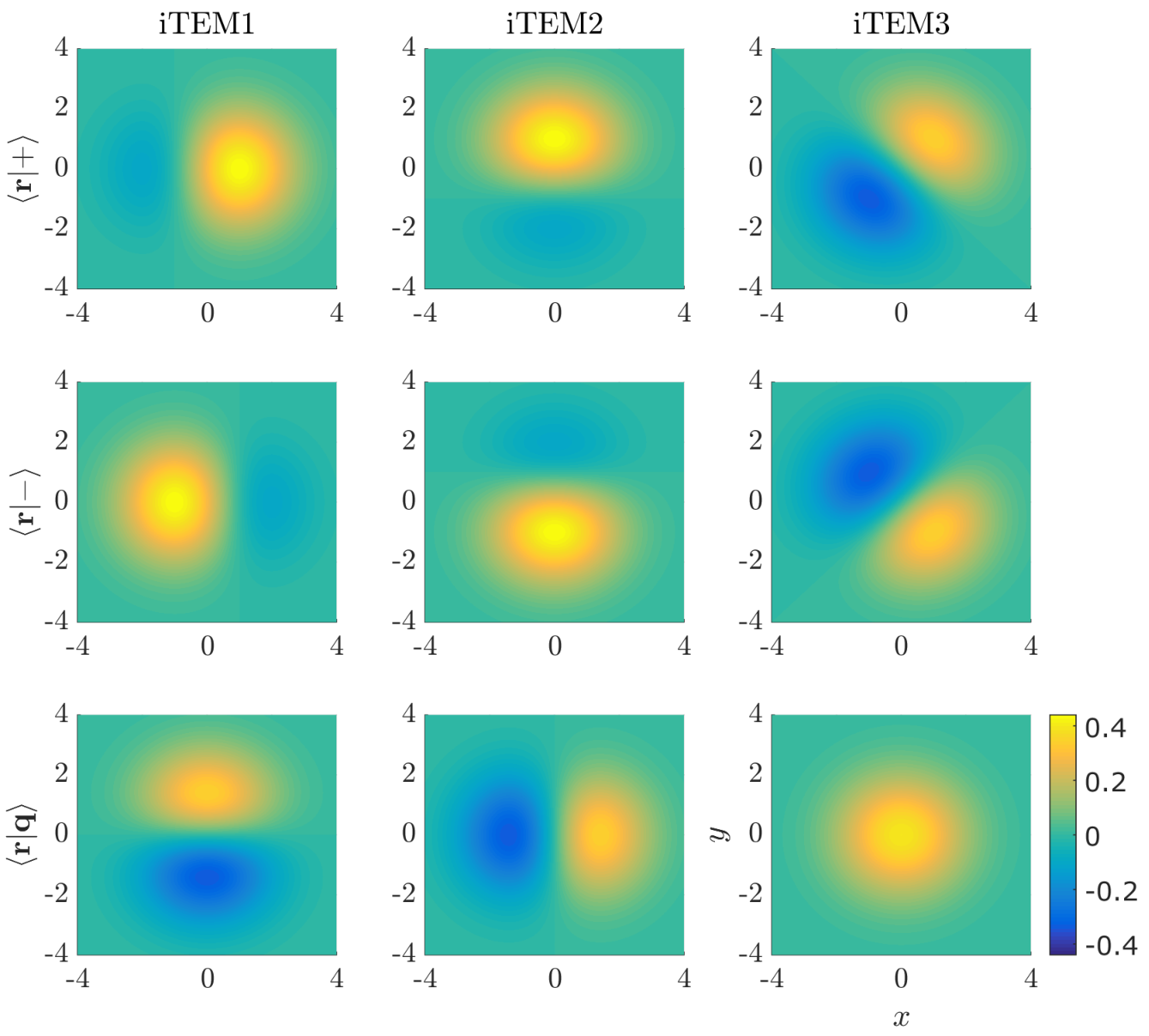

Figure 6 plots the numerically computed mean-square errors (MSEs) for 100 randomly generated objects versus true parameters in log-log scale. Each error value for a given object is computed by averaging the squared difference between the estimator and the true parameter over 500 samples of Poissonian outputs. For comparison, Fig. 6 also plots the CRBs given by Eqs. (27), (30), and (35), assuming and neglecting the term in Eq. (27). A few observations can be made:
- 1.
As shown by the plots in the first row of Fig. 6, SPADE is 3 times worse than direct imaging at estimating the first moments. This is because SPADE uses only 1/3 of the available photons to estimate each first moment.
- 2.
The theory suggests that the advantage of SPADE starts with the second moments, and indeed the other plots show that SPADE is substantially more precise at estimating them, even though SPADE uses only a fraction of the available photons to estimate each moment. This enhancement is a generalization of the recent results on two sources [1, 6, 2, 4, 3, 5, 8, 9, 12, 13, 14, 15].
- 3.
The errors are all remarkably tight to the CRBs, despite the simplicity of the estimators and the approximations in the bounds. In particular, the excellent performance of the SPADE estimator in the subdiffraction regime justifies its assumption of .
VI Quantum limits
In the diffraction-unlimited regime, it is not difficult to prove that direct imaging achieves the highest Fisher information allowed by quantum mechanics. To be precise, that regime can be defined as one in which the PSF is so sharp relative to the source distribution that can be approximated as the orthogonal position basis . becomes diagonal in that basis, and the quantum Fisher information [44, 45, 46, 43, 1, 3] is equal to the direct-imaging information given by Eq. (8). The physics in the opposite subdiffraction regime is entirely different, however, as diffraction causes to have significant overlaps with one another, and more judicious measurements can better deal with the resulting indistinguishability, as demonstrated in Secs. IV and V.
I now prove that SPADE is in fact near-quantum-optimal in estimating location and scale parameters of a source distribution in the subdiffraction regime. Suppose that the distribution has the form
| (40) |
such that parameterizes a coordinate transformation , and the transformation leads to a reference measure that is independent of . Taking as a column vector, I can rewrite Eq. (2) as
| (41) | ||||
| (42) |
where and is the momentum operator in a column vector. I can now use the quantum upper bound on the Fisher information [46, 43, 1] and the convexity of the quantum Fisher information [69, 70] to prove that the Fisher information for any measurement is bounded as
| (43) |
where is the quantum Fisher information proposed by Helstrom [44]. For the pure state, can be computed analytically to give
| (44) | ||||
| (45) |
leading to
| (46) |
for the gaussian PSF. For example, a location parameter can be expressed as . Equation (46) then gives
| (47) |
This can be attained by either direct imaging or iTEM1 in the subdiffraction regime.
The advantage of SPADE starts with the second moments, which are particularly relevant to scale estimation. Let , which results in
| (48) |
For the TEM measurement, on the other hand,
| (49) | ||||
| (50) |
Defining
| (53) | ||||
and using the lower bound by Stein et al. [71], I obtain
| (56) |
which approaches the quantum limit given by Eq. (48) for . The argument can be made more precise if the form of is known, as the extended convexity of the quantum Fisher information can be used to obtain a tighter upper bound [72, 70], while the term in Eq. (VI) can be computed to obtain an explicit lower bound for any .
VII Discussion
Though promising, the giant precision enhancements offered by SPADE do not imply unlimited imaging resolution for finite photon numbers. The higher moments are still more difficult to estimate even with SPADE in terms of the fractional error, which is for even and for odd , meaning that more photons are needed to attain a desirable fractional error for higher-order moments. Intuitively, this is because of the inherent inefficiency of subdiffraction objects to couple to higher-order modes, and the need to accumulate enough photons in those modes to achieve an acceptable SNR. A related issue is the reconstruction of the full source distribution, which requires all moments in principle. A finite number of moments cannot determine the distribution uniquely by themselves [51], although a wide range of regularization methods, such as maximum entropy and basis pursuit, are available for more specific scenarios [51, 73, 74, 55, 57].
Despite these limitations, the fact remains that direct imaging is an even poorer choice of measurement for subdiffraction objects and SPADE can extract much more information, simply from the far field. For example, the size and shape of a star, a planetary system, a galaxy, or a fluorophore cluster that is poorly resolved under direct imaging can be identified much more accurately through the estimation of the second or higher moments by SPADE. Alternatively, SPADE can be used to reach a desirable precision with far fewer photons or a much smaller aperture, enhancing the speed or reducing the size of the imaging system for the more special purposes. In view of the statistical analysis in Refs. [2, 6, 4], the image-inversion interferometers proposed in Refs. [23, 24, 25, 2, 6, 4] are expected to be similarly useful for estimating the second moments. For larger objects, scanning in the manner of confocal microscopy [27] or adaptive alignment [1] should be helpful.
Many open problems remain; chief among them are the incorporation of prior information, generalizations for non-Gaussian PSFs, the derivation of more general quantum limits, the possibility of even better measurements, and experimental implementations. The quantum optimality of SPADE for general imaging is in particular an interesting question. These daunting problems may be attacked by more advanced methods in quantum metrology [44, 45, 46, 43, 75, 76, 77, 78], quantum state tomography [79, 80, 81], compressed sensing [55, 56, 57, 81], and photonics design [52, 53, 54].
Acknowledgments
Inspiring discussions with Ranjith Nair, Xiao-Ming Lu, Shan Zheng Ang, Shilin Ng, Laura Waller’s group, Geoff Schiebinger, Ben Recht, and Alex Lvovsky are gratefully acknowledged. This work is supported by the Singapore National Research Foundation under NRF Grant No. NRF-NRFF2011-07 and the Singapore Ministry of Education Academic Research Fund Tier 1 Project R-263-000-C06-112.
Appendix A Nuisance parameters
Instead of assuming as in Sec. IV, I consider here the exact relation given by Eq. (14), which can be expressed as
| (57) |
For the TEM scheme, this implies that each th channel contains information about not only but also the higher-order moments. If I assume that each th channel is used to estimate only , however, then the higher-order moments act only as nuisance parameters [59] to the estimation of . This is a conservative assumption, as the data-processing inequality [42, 43] implies that neglecting outputs can only reduce the information, but the assumption also means that I do not need to consider any channel with order lower than to compute the CRB with respect to , simplifying the analysis below.
Given the above assumption, I can compute the information matrix with respect to the parameters by considering only the th and higher-order channels; the result is
where and are determined only by the th channel, while is mainly determined by the higher-order channels. The CRB with respect to becomes [59]
| (63) |
The key here is that is smaller than by two orders of , so
| (64) | ||||
| (65) | ||||
| (66) |
which is consistent with Eq. (30).
An intuitive way of understanding this result is to rewrite Eq. (57) as
| (67) |
which implies that the total error in consists of the error in as well as the errors in the higher-order moments. The higher-order moments can be estimated much more accurately via the higher-order channels, so the effect of their uncertainties on the estimation of is negligible. A similar exercise can be done for the iTEM schemes, with similar results.
In practice, such a careful treatment of the nuisance parameters is unlikely to be necessary in the subdiffraction regime, as the numerical analysis in Sec. V shows that excellent results can be obtained simply by taking without any correction.
References
- [1] Mankei Tsang, Ranjith Nair, and Xiao-Ming Lu, “Quantum theory of superresolution for two incoherent optical point sources,” Physical Review X 6, 031033 (2016a).
- [2] Ranjith Nair and Mankei Tsang, “Interferometric superlocalization of two incoherent optical point sources,” Optics Express 24, 3684–3701 (2016a).
- [3] Mankei Tsang, Ranjith Nair, and Xiao-Ming Lu, “Quantum information for semiclassical optics,” in Proc. SPIE, Quantum and Nonlinear Optics IV, Vol. 10029 (2016) p. 1002903.
- [4] Ranjith Nair and Mankei Tsang, “Far-Field Superresolution of Thermal Electromagnetic Sources at the Quantum Limit,” Physical Review Letters 117, 190801 (2016b).
- [5] Mankei Tsang, “Conservative error measures for classical and quantum metrology,” arXiv:1605.03799 [physics, physics:quant-ph] (2016).
- [6] Shan Zheng Ang, Ranjith Nair, and Mankei Tsang, “Quantum limit for two-dimensional resolution of two incoherent optical point sources,” arXiv:1606.00603 [physics, physics:quant-ph] (2016).
- [7] Xiao-Ming Lu, Ranjith Nair, and Mankei Tsang, “Quantum-optimal detection of one-versus-two incoherent sources with arbitrary separation,” arXiv:1609.03025 [quant-ph] (2016).
- [8] Cosmo Lupo and Stefano Pirandola, “Ultimate Precision Bound of Quantum and Subwavelength Imaging,” Physical Review Letters 117, 190802 (2016).
- [9] J. Rehacek, M. Paúr, B. Stoklasa, Z. Hradil, and L. L. Sánchez-Soto, “Optimal measurements for resolution beyond the Rayleigh limit,” Optics Letters 42, 231–234 (2017).
- [10] Hari Krovi, Saikat Guha, and Jeffrey H. Shapiro, “Attaining the quantum limit of passive imaging,” arXiv:1609.00684 [physics, physics:quant-ph] (2016).
- [11] Ronan Kerviche, Saikat Guha, and Amit Ashok, “Fundamental limit of resolving two point sources limited by an arbitrary point spread function,” arXiv:1701.04913 [physics, physics:quant-ph] (2017).
- [12] Zong Sheng Tang, Kadir Durak, and Alexander Ling, “Fault-tolerant and finite-error localization for point emitters within the diffraction limit,” Optics Express 24, 22004 (2016).
- [13] Fan Yang, Arina Tashchilina, E. S. Moiseev, Christoph Simon, and A. I. Lvovsky, “Far-field linear optical superresolution via heterodyne detection in a higher-order local oscillator mode,” Optica 3, 1148 (2016).
- [14] Weng Kian Tham, Hugo Ferretti, and Aephraim M. Steinberg, “Beating Rayleigh’s Curse by Imaging Using Phase Information,” arXiv:1606.02666 [physics, physics:quant-ph] (2016), accepted by Physical Review Letters.
- [15] Martin Paúr, Bohumil Stoklasa, Zdenek Hradil, Luis L. Sánchez-Soto, and Jaroslav Rehacek, “Achieving the ultimate optical resolution,” Optica 3, 1144 (2016).
- [16] E. Bettens, D. Van Dyck, A. J. den Dekker, J. Sijbers, and A. van den Bos, “Model-based two-object resolution from observations having counting statistics,” Ultramicroscopy 77, 37–48 (1999).
- [17] S. Van Aert, A. J. den Dekker, D. Van Dyck, and A. van den Bos, “High-resolution electron microscopy and electron tomography: resolution versus precision,” Journal of Structural Biology 138, 21–33 (2002).
- [18] Sripad Ram, E. Sally Ward, and Raimund J. Ober, “Beyond Rayleigh’s criterion: A resolution measure with application to single-molecule microscopy,” Proceedings of the National Academy of Sciences of the United States of America 103, 4457–4462 (2006).
- [19] Carmen O. Acuna and Joseph Horowitz, “A statistical approach to the resolution of point sources,” Journal of Applied Statistics 24, 421–436 (1997).
- [20] J. G. Walker, G. J. Brakenhoff, M. Bertero, E. R. Pike, R. E. Davies, and M. R. Young, “Superresolving scanning optical microscopy using holographic optical processing,” J. Opt. Soc. Am. A 10, 59–64 (1993).
- [21] F. Tamburini, G. Anzolin, G. Umbriaco, A. Bianchini, and C. Barbieri, “Overcoming the Rayleigh Criterion Limit with Optical Vortices,” Physical Review Letters 97, 163903 (2006).
- [22] Nicolas Sandeau and Hugues Giovannini, “Increasing the lateral resolution of 4pi fluorescence microscopes,” Journal of the Optical Society of America A 23, 1089 (2006).
- [23] Kai Wicker and Rainer Heintzmann, “Interferometric resolution improvement for confocal microscopes,” Optics Express 15, 12206 (2007).
- [24] Kai Wicker, Simon Sindbert, and Rainer Heintzmann, “Characterisation of a resolution enhancing image inversion interferometer,” Optics Express 17, 15491 (2009).
- [25] D. Weigel, R. Foerster, H. Babovsky, A. Kiessling, and R. Kowarschik, “Enhanced resolution of microscopic objects by image inversion interferometry,” Optics Express 19, 26451 (2011).
- [26] Richard J. Prokop and Anthony P. Reeves, “A survey of moment-based techniques for unoccluded object representation and recognition,” CVGIP: Graphical Models and Image Processing 54, 438–460 (1992).
- [27] James B. Pawley, ed., Handbook of Biological Confocal Microscopy (Springer, New York, 2006).
- [28] Hendrik Deschout, Francesca Cella Zanacchi, Michael Mlodzianoski, Alberto Diaspro, Joerg Bewersdorf, Samuel T. Hess, and Kevin Braeckmans, “Precisely and accurately localizing single emitters in fluorescence microscopy,” Nature Methods 11, 253–266 (2014).
- [29] Kim I. Mortensen, L. Stirling Churchman, James A. Spudich, and Henrik Flyvbjerg, “Optimized localization analysis for single-molecule tracking and super-resolution microscopy,” Nature Methods 7, 377–381 (2010).
- [30] Jerry Chao, E. Sally Ward, and Raimund J. Ober, “Fisher information theory for parameter estimation in single molecule microscopy: tutorial,” Journal of the Optical Society of America A 33, B36 (2016).
- [31] Martin C. E. Huber, Anuschka Pauluhn, J. Len Culhane, J. Gethyn Timothy, Klaus Wilhelm, and Alex Zehnder, eds., Observing Photons in Space: A Guide to Experimental Space Astronomy (Springer, New York, 2013).
- [32] J. C. Christou, G. Brusa, A. Conrad, S. Esposito, T. Herbst, P. Hinz, J. M. Hill, D. L. Miller, S. Rabien, G. Rahmer, G. E. Taylor, C. Veillet, and X. Zhang, “Adaptive optics capabilities at the Large Binocular Telescope Observatory,” in Proc. SPIE, Adaptive Optics Systems V, Vol. 9909 (2016) p. 99092E.
- [33] Gary H. Sanders, “The Thirty Meter Telescope (TMT): An International Observatory,” Journal of Astrophysics and Astronomy 34, 81–86 (2013).
- [34] Rebecca A. Bernstein et al., “Overview and status of the Giant Magellan Telescope project,” in Proc. SPIE, Ground-based and Airborne Telescopes V, Vol. 9145 (2014) p. 91451C.
- [35] R. Davies et al., “MICADO: first light imager for the E-ELT,” in Proc. SPIE, Ground-based and Airborne Instrumentation for Astronomy VI, Vol. 9908 (2016) p. 99081Z.
- [36] Jonas Zmuidzinas, “Cramér–Rao sensitivity limits for astronomical instruments: implications for interferometer design,” J. Opt. Soc. Am. A 20, 218–233 (2003).
- [37] Joseph W. Goodman, Statistical Optics (Wiley, New York, 1985).
- [38] Joseph W. Goodman, Introduction to Fourier Optics (McGraw-Hill, New York, 2004).
- [39] Jeffrey H. Shapiro, “The quantum theory of optical communications,” IEEE Journal of Selected Topics in Quantum Electronics 15, 1547–1569 (2009).
- [40] Larry A. Wasserman, All of Statistics (Springer, New York, 2004).
- [41] Harry L. Van Trees, Detection, Estimation, and Modulation Theory, Part I. (John Wiley & Sons, New York, 2001).
- [42] Ram Zamir, “A proof of the Fisher information inequality via a data processing argument,” IEEE Transactions on Information Theory 44, 1246–1250 (1998).
- [43] M. Hayashi, Quantum Information (Springer, Berlin, 2006).
- [44] Carl W. Helstrom, Quantum Detection and Estimation Theory (Academic Press, New York, 1976).
- [45] Alexander S. Holevo, Probabilistic and Statistical Aspects of Quantum Theory (Edizioni della Normale, Pisa, Italy, 2011).
- [46] Masahito Hayashi, ed., Asymptotic Theory of Quantum Statistical Inference: Selected Papers (World Scientific, Singapore, 2005).
- [47] Amnon Yariv, Quantum Electronics (Wiley, New York, 1989).
- [48] DLMF, “NIST Digital Library of Mathematical Functions,” http://dlmf.nist.gov/, Release 1.0.11 of 2016-06-08, online companion to [49].
- [49] Frank W. J. Olver, Daniel W. Lozier, Ronald F. Boisvert, and Charles W. Clark, eds., NIST Handbook of Mathematical Functions (Cambridge University Press, New York, NY, 2010) print companion to [48].
- [50] Leonard Mandel and Emil Wolf, Optical Coherence and Quantum Optics (Cambridge University Press, Cambridge, 1995).
- [51] M. Bertero, “Linear Inverse and III-Posed Problems,” in Advances in Electronics and Electron Physics, Vol. 75, edited by Peter W. Hawkes (Academic Press, 1989) pp. 1–120.
- [52] Seiji Armstrong, Jean-Francois Morizur, Jiri Janousek, Boris Hage, Nicolas Treps, Ping Koy Lam, and Hans-A. Bachor, “Programmable multimode quantum networks,” Nature Commun. 3, 1026 (2012).
- [53] David A. B. Miller, “Self-configuring universal linear optical component [Invited],” Photonics Research 1, 1–15 (2013).
- [54] Guifang Li, Neng Bai, Ningbo Zhao, and Cen Xia, “Space-division multiplexing: the next frontier in optical communication,” Advances in Optics and Photonics 6, 413–487 (2014).
- [55] Yohann de Castro and Fabrice Gamboa, “Exact reconstruction using Beurling minimal extrapolation,” Journal of Mathematical Analysis and Applications 395, 336–354 (2012).
- [56] Emmanuel J. Candès and Carlos Fernandez-Granda, “Towards a Mathematical Theory of Super-resolution,” Communications on Pure and Applied Mathematics 67, 906–956 (2014).
- [57] Geoffrey Schiebinger, Elina Robeva, and Benjamin Recht, “Superresolution without Separation,” arXiv:1506.03144 [cs, math] (2015).
- [58] D. R. Cox and N. Reid, “Parameter Orthogonality and Approximate Conditional Inference,” Journal of the Royal Statistical Society. Series B (Methodological) 49, 1–39 (1987).
- [59] Harry L. Van Trees and Kristine L. Bell, eds., Bayesian Bounds for Parameter Estimation and Nonlinear Filtering/Tracking (Wiley-IEEE, Piscataway, 2007).
- [60] Antoine Labeyrie, Stephen G. Lipson, and Peter Nisenson, An Introduction to Optical Stellar Interferometry (Cambridge University Press, Cambridge, 2006).
- [61] William E. Moerner, “New directions in single-molecule imaging and analysis,” Proceedings of the National Academy of Sciences 104, 12596–12602 (2007).
- [62] Eric Betzig, George H. Patterson, Rachid Sougrat, O. Wolf Lindwasser, Scott Olenych, Juan S. Bonifacino, Michael W. Davidson, Jennifer Lippincott-Schwartz, and Harald F. Hess, “Imaging intracellular fluorescent proteins at nanometer resolution,” Science 313, 1642–1645 (2006).
- [63] Stefan W. Hell, “Far-field optical nanoscopy,” Science 316, 1153–1158 (2007).
- [64] Mikhail I. Kolobov, ed., Quantum Imaging (Springer, New York, 2007).
- [65] Michael A. Taylor, Jiri Janousek, Vincent Daria, Joachim Knittel, Boris Hage, Hans-A. Bachor, and Warwick P. Bowen, “Biological measurement beyond the quantum limit,” Nature Photonics 7, 229–233 (2013).
- [66] Mankei Tsang, “Quantum limits to optical point-source localization,” Optica 2, 646–653 (2015).
- [67] J. B. Pendry, “Negative Refraction Makes a Perfect Lens,” Physical Review Letters 85, 3966–3969 (2000).
- [68] Mankei Tsang and Demetri Psaltis, “Magnifying perfect lens and superlens design by coordinate transformation,” Physical Review B 77, 035122 (2008).
- [69] Akio Fujiwara, “Quantum channel identification problem,” Physical Review A 63, 042304 (2001).
- [70] Shilin Ng, Shan Zheng Ang, Trevor A. Wheatley, Hidehiro Yonezawa, Akira Furusawa, Elanor H. Huntington, and Mankei Tsang, “Spectrum analysis with quantum dynamical systems,” Physical Review A 93, 042121 (2016).
- [71] M. Stein, A. Mezghani, and J. A. Nossek, “A Lower Bound for the Fisher Information Measure,” IEEE Signal Processing Letters 21, 796–799 (2014).
- [72] S. Alipour and A. T. Rezakhani, “Extended convexity of quantum fisher information in quantum metrology,” Phys. Rev. A 91, 042104 (2015).
- [73] S. F. Gull and J. Skilling, “Maximum entropy method in image processing,” IEE Proceedings F - Communications, Radar and Signal Processing 131, 646–659 (1984).
- [74] P. Milanfar, W. C. Karl, and A. S. Willsky, “A moment-based variational approach to tomographic reconstruction,” IEEE Transactions on Image Processing 5, 459–470 (1996).
- [75] Jonas Kahn and Mădălin Guţă, “Local Asymptotic Normality for Finite Dimensional Quantum Systems,” Communications in Mathematical Physics 289, 597–652 (2009).
- [76] Dominic W. Berry, Mankei Tsang, Michael J. W. Hall, and Howard M. Wiseman, “Quantum Bell-Ziv-Zakai Bounds and Heisenberg Limits for Waveform Estimation,” Phys. Rev. X 5, 031018 (2015).
- [77] Xiao-Ming Lu and Mankei Tsang, “Quantum Weiss-Weinstein bounds for quantum metrology,” Quantum Science and Technology 1, 015002 (2016).
- [78] Christos N. Gagatsos, Dominic Branford, and Animesh Datta, “Gaussian systems for quantum-enhanced multiple phase estimation,” Physical Review A 94, 042342 (2016).
- [79] Miroslav Ježek and Zdeněk Hradil, “Reconstruction of spatial, phase, and coherence properties of light,” Journal of the Optical Society of America A 21, 1407 (2004).
- [80] A. I. Lvovsky and M. G. Raymer, “Continuous-variable optical quantum-state tomography,” Reviews of Modern Physics 81, 299–332 (2009).
- [81] David Gross, Yi-Kai Liu, Steven T. Flammia, Stephen Becker, and Jens Eisert, “Quantum state tomography via compressed sensing,” Phys. Rev. Lett. 105, 150401 (2010).