A Mid-level Planning System for
Object Reorientation

Weiwei Wan Hisashi Igawa Kensuke Harada Zepei Wu Hiromu Onda Kazuyuki Nagata Natsuki Yamanobe ^†^†thanks: Weiwei Wan, Kensuke Harada, Zepei Wu, Kazuyuki Nagata, Hiromu Onda, and Natsuki Yamanobe are with National Institute of Advanced Industrial Science and Technology (AIST), Japan. Hisashi Igawa is with Hokkaido Research Organization, Japan. Kensuke Harada is also affiliated with Osaka University, Japan. Zepei Wu is also affiliated with Tsukuba University. wan-weiwei@aist.go.jp

Abstract

This paper presents a mid-level planning system for object reorientation. It includes a grasp planner, a placement planner, and a regrasp sequence solver. Given the initial and goal poses of an object, the mid-level planning system finds a sequence of hand configurations that reorient the object from the initial to the goal. This mid-level planning system is open to low-level motion planning algorithm by providing two end-effector poses as the input. It is also open to high-level symbolic planners by providing interface functions like placing an object to a given position at a given rotation. The planning system is demonstrated with several simulation examples and real-robot executions using a Kawada Hiro robot and Robotiq 85 grippers.

Index Terms:

Grasp Planning, Manipulation Planning, Object Reorientation

I Introduction

Refer to caption — Fig. 1: Some tasks that require object reorientation. (a) Packing objects. The task requires reorienting objects in (a.1) into the poses in (a.2). (b) Assembly. The task requires reorienting the capacitors in (b.1) into the poses in (b.2) and inserts them. (c) Using tools. The task requires reorienting the wrench in (c.1) into the pose in (c.2) so that its jaw fits into the nut.

Object reorientation is a common manipulation task for robots. Given an initial pose of an object, a reorientation task requires a robot to pick up the object, reorient it into a predefined pose, and place it down at a certain position.

Some typical tasks that require object reorientation are shown in Fig.1. The first one is a packing task. To finish this task, a robot is required to reorient the object into the expected poses and pack them into the box. The second one is an assembly task. A robot is required to reorient the capacitor into the expected pose and insert it into the base. The last one is to fastening a nut using a wrench. A robot must reorient the wrench to have its jaw fit into the nut. All these tasks are essentially object reorientation tasks.

The paper develops algorithms to plan the motions that robots need to perform object reorientation. It presents a mid-level planning system which includes a grasp planner, a placement planner, and a regrasp sequence solver. The input to the mid-level system is a sequence of goal poses of the objects planned by a high-level assembly or symbolic planning component. The output of the mid-level system is a sequence of robot poses and grasp configurations that will be used by a low-level motion planning component. Given the initial and goal poses of an object, the mid-level system finds a sequence of robot poses and hand configurations that reorients the object from the initial to the goal. This mid-level system is open to low-level motion planning algorithms by providing two end-effector poses as the start and goal. It is also open to high-level symbolic or assembly planners by providing an interface function like placing an object to a given position at a given rotation.

The essence of the mid-level planning system is a regrasp planner which uses the stable placements of objects to increase the connectivity of grasp configurations. To reorient the poses, a robot may place down the object at intermediate placements and regrasp them. The regrasp reduces the constraints from obstacles and robot kinematics.

The concept of mid-level planning system is novel in robotic planning community. We in this paper develop a library that plays the role of the mid-level system and demonstrate its efficacy with both simulation and real-world experiments using a Kawada Hiro¹¹ 1 http://nextage.kawada.jp/en/ robot and Robotiq 85 grippers. The source code is available on GitHub²² 2 https://github.com/wanweiwei07/hiromatlab.

The terminologies used are as follows. “Object pose” is used to refer to the position and orientation of an object. “Robot pose” is used to refer to a set of joint angles of the robot. “Grasp configuration” and “regrasp configuration” are used to refer to a set of hand position, hand orientation and hand joint angles.

II Background and Related Work

The position of a mid-level planning system in a planning platform is shown in Fig.2. In the highest level, the planning focuses on symbolic and logical aspects. Examples include AND/OR graph assembly planning[1], geometric and physical reasoning [2, 3], symbolic deduction[4, 5], etc. The high-level planners analyze the contacts between objects, divide a task into sub-tasks, and decide the order of operation. The output of the high-level component is usually a sequence of goal poses of objects. In the low level, the planning focuses on the motion between two configurations. Examples include probabilistic methods like Probabilistic Roadmap (PRM)[6], Rapidly-epxloring Random Tree (RRT)[7], etc., and optimization-based methods like Covariant Hmiltonian Optimization for Motion Planning (CHOMP)[8], TrajOpt[9], etc. The low-level planners generate trajectories of robots that avoid collision with obstacles and fulfill dynamic constraints. The mid-level planning system takes the sequence of objects’ goal poses computed in the high-level component, computes a sequence of robot poses and grasp configurations, and sends them to the low-level motion planner to find feasible motions. This paper focuses on the mid-level aspect. It proposes the concept of mid-level planning and develops libraries and real-world systems to demonstrate the concept.

To our best knowledge, the concept of mid-level planning is not strictly defined, although related studies have been performed for decades. The most relevant work is integrated task and motion planning. The first integrated task and motion planning system is the STRIPS used in the Shakey robot [10], which presented an integrated symbolic deduction and movement planning system for a mobile robot. Following this seminal study, much work has been devoted to the integrated task and motion planning for mobile platforms. A good summary and discussion of the open problems before 2007 could be found in [11]. More recent work like [12] considers temporal constraints and uncertainty in the environments. Integrated planners are employed iteratively to generate safe motions for mobile robots to finish office traversing tasks. [13] also does integrated task and motion planning while considering temporal constraints and uncertainty. The task is distributed to multiple robots. The sequence of executions as well as motions are planned. [14] only considers temporal constraints in the integration and applies the integrated symbolic deduction and planning to plan the motions of mobile robots in the presence of moving obstacles. [15] considers temporal constraints and applies the integrated planning to scenarios like crew planning (multiple mobile robots) and room scanning. These integrated planning in [12, 13, 14, 15] are about the tasks of mobile robots. The high-level planner finds motion sequences and the low-level planner finds collision-free trajectories. Key poses of the mobile robots that connect the high-level and low-level results are on a middle layer, which is although implicit.

The planning systems on the tasks of manipulators also has an implicit middle layer. [16] presents an integrated assembly and motion planning system which employs several mobile manipulators to assemble a chair. The system has a high-level assembly sequence solver and a low-level robot motion planner. The paper didn’t explicitly claim a mid-level solver but was actually using it to plan robot poses and grasp configurations. [17] iteratively plans robot tasks and motions considering geometric constraints in the environment. The system implicitly uses some mid-level planners to plan the robot poses and grasp confiugrations considering preconditions. [18] presents an integrated planning system which plans assembly sequences using geometric reasoning, plans coordinated manipulation sequences using symbolic deduction, and plans robot poses and grasp configurations considering each manipulation sequence [19] and robot motions using sampling-based methods [20]. The assembly sequences and coordinated manipulation sequences are the result of high-level planners, the robot motions are the results of low-level planners. The robot poses and grasp configurations are on a middle layer which is between the high-level and low-level results. [21] presents an integrated symbolic deduction system which integrates viewpoint planning, state estimation, and action planning. The advantage is that uncertainty is considered when dealing with various geometric constraints. Again, the robot poses and grasp configurations are in a middle level. [22] presents a similar integrated symbolic deduction and action planning planning system. The concept of motion grammar is proposed as the high-level interface. The touching poses are also the results of some middle level planners. [23] presents an integrated task and PRM motion planner which simultaneously samples in the sub-task space and transition space. The transition space is actually what a mid-level planner should explore. Many other studies like [24, 25, 26, 27, 28, 29] are also implicitly employing some mid-level planners.

This paper explicitly develops a mid-level planning system for object reorientation. Like the literature on integrated task and motion planning, the sequences planned by our mid-level system are robot poses and grasp configurations. The essence the mid-level planning system is a regrasp planner which uses the stable placements of objects to increase the connectivity of grasp configurations. The seminal study of regrasp planning is [30] which builds a grasp-placement table (GP) and searches the table to find a sequence of grasping and releasing key poses for object reorientation. Some ensuing work that also uses search tables includes [31, 32, 33, 34] which concentrates on industrial grippers and [35, 36] which applies regrasp to dexterous hands. The most up-to-date study based on the same idea is [37]. Other work like [38, 39, 40, 41, 42] also do regrasp planning but the focus is more on planning of the sequences rather than object reorientation. Our group published several articles on regrasp [43, 44, 45]. These studies are based on graph search rather than tables. Graph search has much higher performance and makes it possible to plan dual-arm or multi-arm regrasps [46, 47, 48]. This paper further develops our graph-based regrasp planner and uses it to construct a mid-level planning system. The system has interfaces to the high-level assembly or symbolic planners and low-level motion planners, and is demonstrated with various object reorientation tasks like packing objects, assembly, and using tools.

III System Overview

Fig.3 shows an overview of the mid-level planning system. The colored boxes in it correspond to the ones marked with the same colors in Fig.2. The mid-level planning system includes a grasp planner, a placements planner, and a regrasp sequence solver which are marked with red, green, and blue respectively. The input to the system includes the goal poses of the object and the kinematic parameters of the robots, which are shown in the upper-right corner of Fig.2.

First, the system computes the force-closure grasps of an object using its geometric model and the model of a given robotic gripper in the grasp planner. Collision with obstacles are not considered in step. The output is a set of poses and configurations of the gripper described in the object’s local coordinate system. Then, in the placement planner, the system finds the placements of the object by computing its convex hull and checks on which facet of the convex hull can the object stand stably. Each stable stand is one placement and is described in the world coordinate system. The force-closure grasps computed in the first step will be associated with the placements using coordinate transformation between world coordinate system and the object’s local coordinate system, and collision detection with obstacles in the environment. The output of the placement planner is the stable placements of the object together with the accessible grasps to hold the placements. The regrasp sequence solver uses the placements and their accessible grasps to find a sequence of robot poses and grasp configurations that reorient the object from a given start to a given goal. The initial pose of the object is assumed to be obtained from a vision system. The goal poses of the object and the kinematic parameters of the robot are input to the system by human beings. The input are used together with the placements and their accessible grasps to build a regrasp graph. The algorithms search the graph to compute a sequence of robot poses and grasp configurations.

This mid-level planning system is open to low-level motion planning algorithm by providing robot poses and grasp configurations as the start and goal. The output of the system is a sequence of robot poses and grasp configurations. Each adjacent pair of the poses and configurations will be used as the start and goal of a motion planning algorithm which provides direct interface to low level motion planners. On the other hand, the system is open to high-level symbolic planners by providing interface functions like placing an object to a given position at a given pose. The input to the system is the initial and goal poses of the object. The system solves regrasp sequences and decides the grasp and regrasp configurations by itself in this mid-level. It blinds programmers from both itself and the low-level motion planning details.

IV Implementation Details

This section introduces the implementation details of each part shown in Fig.3.

IV-A Grasp planner

We use the same grasp planning algorithm presented in [43]. The robotic hand is supposed to be an industrial gripper (Robotiq 85³³ 3 http://robotiq.com/products/adaptive-robot-gripper/). The process is done without considering external collisions. Only the collision detection between the hands and the object is performed to ensure feasibility. The output of the grasp planner is a set $\textbf{G}=\{\textit{{g}}_{1},\textit{{g}}_{2},\ldots,\textit{{g}}_{n}\}$ where an element $\textit{{g}}_{x}=\{p_{x},R_{x},\textit{{j}}_{x}\}$ . Here, the tuple $(p_{x},R_{x})$ indicates the position and orientation of the robotic gripper. The vector $\textit{{j}}_{x}$ indicates the angles of each finger joints. Each $\textit{{g}}_{x}$ is computed following the requirements of force closure using a predefined friction coefficient. Collision detection is performed between $\textit{{g}}_{x}$ and the mesh model M to ensure a grasp doesnt collide the object.

Fig.4 shows the result of the grasp planner. Each grasp is represented by a segment plus a coordinate system attached to the end of the segment as shown in Fig.4(c) and (d). The end of the segment is the $p_{x}$ . The coordinate system implies the $R_{x}$ . The $\textit{{j}}_{x}$ is not illustrated.

IV-B Placement planner

Placement planner plans the stable placements of an object on a table surface and associates the accessible grasps to the placements. We are using an improved version of the placement planner presented in [48]. In the previous work, the placement planner computes the convex hull of the object and checks on which facet of the convex hull can the object stand stably. Each stable stand is treated as one placement of the object. Grasps are associated with a placement considering collision with a horizontal supporting surface, which is the only obstacles taken into account. In this improved version, we allow arbitrary obstacles. Like the previous work, we compute the convex hull of the objects mesh model, and find its stable placements on table surfaces. The difference is we allow taking any rigid body obstacles into account. When associating the grasps, we could not only specify a horizontal surface as an obstacle, but also arbitrary rigid mesh models in the environment.

The output of the placement planner is a set $\textbf{P}=\{\textit{{p}}_{1},\textit{{p}}_{2},\ldots,\textit{{p}}_{n}\}$ where an element $\textit{{p}}_{i}=\{(p_{i})^{p},(R_{i})^{p},(\textbf{G}_{i})^{p}\}$ . Here, $((p_{i})^{p},(R_{i})^{p})$ indicates the position and orientation of the object. $(\textbf{G}_{i})^{p}$ indicates the accessible force-closure and collision-free grasps that associate with the object resting at pose $((p_{i})^{p},(R_{i})^{p})$ . $(\textbf{G}_{i})^{p}=\{(\textit{{g}}_{i1})^{p},(\textit{{g}}_{i2})^{p},\ldots,(\textit{{g}}_{in})^{p}\}$ where each $(\textit{{g}}_{ix})^{p}$ is basically an element from the set G computed by the grasp planner. It is transformed to the coordinates of $\textit{{p}}_{i}$ using $(\textit{{g}}_{ix})^{p}=(R_{i})^{p}\cdot\textit{{g}}_{x}+(p_{i})^{p}$ . Collision detection is performed between $(\textit{{g}}_{ix})^{p}$ and the obstacles in the environment. Obstacles could be the supporting table surfaces and some surrounding objects in the environment.

Fig.5 shows the placements of the object in Fig.4(a). The object can stand on a table with six stable placements. The grasps associated with the placements are shown using segments. The coordinates attached to the end of segment are removed to ensure better visualization. There are no obstacles surrounding the placements and collision detection is only performed between $(\textit{{g}}_{ix})^{p}$ and the table surface. The collided grasps are inaccessible and are not associated with the placements.

Fig.6(b) shows the cases where surrounding obstacles exist. The gray block is supposed to be an obstacle. As the obstacle changes its position, the accessible grasps associated with the object change correspondently. Collision detection is only between both $(\textit{{g}}_{ix})^{p}$ and the table surface, and both $(\textit{{g}}_{ix})^{p}$ and the obstacle.

IV-C Regrasp sequence solver

The regrasp sequence solver uses the placements and their associated grasps to find a sequence of robot poses and grasp configurations that reorient the object from a given start to a given goal. In implementation, the solver further examines the accessible grasps considering the kinematics of a robot and motion primitives[49, 50], builds a two-layer regrasp graph, connects the start and goal to the graph, and searches the graph.

IV-C1 Kinematics of the robot

The grasps in previous sub-sections are computed without considering robot kinematics. Before building the graph and searching for a regrasp sequence, the grasps are further examined to ensure the accessibility to specific robots. The flowchart in Fig.7 shows how the examinations are performed.

Given a position $p$ on the table, the algorithm moves the placements to it and checks the collision with surrounding obstacles. This collision detection step is marked with red shadow in Fig.7. Collided grasps at the new $p$ are removed by this step. Then, for each of the remaining grasps, the algorithm checks the feasibility of the robot’s IK by posing its end effector at them. The IK-infeasible grasps are also removed. The output of the algorithm is still a set $\textbf{P}=\{\textit{{p}}_{1},\textit{{p}}_{2},\ldots,\textit{{p}}_{n}\}$ where an element $\textit{{p}}_{i}=\{(p_{i})^{p},(R_{i})^{p},(\textbf{G}_{i})^{p}\}$ . Nevertheless, the $(p_{i})^{p}$ is set to the newly given $p$ and the elements of $(\textbf{G}_{i})^{p}$ are both collision-free and IK-feasible.

Fig.8 shows an example. A placement and its associated grasps without considering robotic kinematics is shown in Fig.8(a). In contrast, the placement and its associated grasps at a position in front of a Kawada Hiro robot, shown in Fig.8(c)) is shown in Fig.8(b). The IK-infeasible grasps are removed.

IV-C2 Incorporating motion primitives

Motion primitives are defined as two sequential IK-feasible grasps. Fig.9 shows the four motion primitives used in the paper. It includes: Fig.9(a) A grasp primitive, which includes a pregrasp key pose and a grasp key pose. The object pose doesn’t change in the primitive; Fig.9(b) A release primitive, which includes a grasp key pose and a pregrasp key pose. It is the inverse of (a) and the object pose doesn’t change; Fig.9(c) A picking-up primitive, which includes a grasp key pose and a retraction key pose. The object retracts together with the retraction key pose in the primitive; Fig.9(d) A placing-down primitive. It is the inverse of (c). The reason to incorporate motion primitive is to relax motion planning. Without considering the primitives, the robot has to plan a motion between the initial and goal states shown in Fig.10(a) which involves contacts between the object and the table surface in workspace and narrow or highly constrained configuration spaces in configuration space [51, 52]. Motion primitives relaxes the planning around the narrow configuration spaces. A robot only needs to plan between two intermediate states. The motion between the intermediate states and the initial and goal states are defined by the primitives. An example is shown in Fig.10(b), the picking-up and placing-down motion primitives take care of the motion between the intermediate states (red plots) and the initial and goal states, leaving motion planners to find a motion between the intermediate states.

Incorporating motion primitives requires further examining their feasibility. For a grasp $\textit{{g}}_{x}=(p_{x},R_{x},\textit{{j}}_{x})$ , the grasp and release motion primitives are defined as ( $(p_{x},R_{x},\textit{{j}}_{x})$ , $(p_{x}+\omega[R_{x}(1,1),R_{x}(2,1),R_{x}(3,1)],R_{x},\textit{{j}}_{x})$ ) and ( $(p_{x}+\omega[R_{x}(1,1),R_{x}(2,1),R_{x}(3,1)],R_{x},\textit{{j}}_{x})$ , $(p_{x},R_{x},\textit{{j}}_{x})$ ) where $[R_{x}(1,1),R_{x}(2,1),R_{x}(3,1)]$ is the approaching direction of the robot gripper. $\omega$ controls the scale of the primitive. The picking-up and placing-down motion primitives are defined as ( $(p_{x},R_{x},\textit{{j}}_{x})$ , $(p_{x}+\omega\cdot backward,R_{x},\textit{{j}}_{x})$ ) and ( $(p_{x}+\omega\cdot backward,R_{x},\textit{{j}}_{x})$ , $(p_{x},R_{x},\textit{{j}}_{x})$ ) where $backward$ is planned by a high-level planner. If $backward$ is the upward direction $[0,0,1]$ , the picking-up and placing-down motion primitives are exactly along the up-down direction. $\omega$ is the same controlling parameter. The IK at $(p_{x}+\omega\cdot[R_{x}(1,1),R_{x}(2,1),R_{x}(3,1)],R_{x},\textit{{j}}_{x})$ and $(p_{x}+\omega\cdot backward,R_{x},\textit{{j}}_{x})$ are further examined to ensure the four motion primitives are feasible. After incorporating motion primitives, each element of the placement is saved as a triple $\textit{{p}}_{i}=(\textit{{p}}_{i}^{o},\textit{{p}}_{i}^{pre},\textit{{p}}_{i}^{ret})$ where $\textit{{p}}_{i}^{o}$ is the original placement and its associated grasps, $\textit{{p}}_{i}^{pre}$ is the placement with the grasps for grasp and release motion primitives, and $\textit{{p}}_{i}^{ret}$ is the placement with the grasps for picking-up and placing-down motion primitives.

Fig.11 shows the results after further reducing the IK-infeasible grasps considering motion primitives. Comparing with Fig.8 the number of accessible grasps are further decreased. Fig.11(b) and (d) correspond to $\textit{{p}}_{i}^{o}$ . Fig.11(a) corresponds to $\textit{{p}}_{i}^{pre}$ . Fig.11(c) corresponds to $\textit{{p}}_{i}^{ret}$ .

IV-C3 The two-layer regrasp graph

The regrasp graph connects the placements using the shared grasps. For two placements $\textit{{p}}_{i}$ and $\textit{{p}}_{j}$ (more exactly $\textit{{p}}_{i}^{o}$ and $\textit{{p}}_{j}^{o}$ ), if $\exists\textit{{g}}_{x}$ where $(R_{i})^{p}\cdot\textit{{g}}_{x}+(p_{i})^{p}\in\textbf{G}_{i}$ and $(R_{j})^{p}\cdot\textit{{g}}_{x}+(p_{j})^{p}\in\textbf{G}_{j}$ , they can be connected. It means there exists a shared grasp that is identical in the objects local coordinate system and is associated with both placements. A robot could pick up the object resting at $\textit{{p}}_{i}$ using a grasp $\textit{{g}}_{ix}=(R_{i})^{p}\cdot\textit{{g}}_{x}+(p_{i})^{p}$ , transforms its end effector pose to $(p_{j},R_{j})$ , and places the object down with the grasp $\textit{{g}}_{jx}=(R_{j})^{p}\cdot\textit{{g}}_{x}+(p_{j})^{p}$ .

Fig.12(a) shows this shared grasp using a red segment. These two placements in the figure are represented as two rectangular nodes and are connected with each other (see the right part of (a)). This connection is in the first layer which only shows whether two placements are connectible. The two rectangular nodes correspond to ( $p_{i}$ , $R_{i}$ ) and ( $p_{j}$ , $R_{j}$ ) respectively. Grasps are not involved. The second layer of the graph further shows the number of shared grasps. See Fig.12(b) for examples. The two placements share many grasps (see the red segments). Each shared grasp leads to one segment between the two placements in the second layer. The two circular nodes at the end of the segment correspond to $(R_{i})^{p}\cdot\textit{{g}}_{x_{k}}+(p_{i})^{p}$ and $(R_{j})^{p}\cdot\textit{{g}}_{x_{k}}+(p_{j})^{p}\in\textbf{G}_{j}$ respectively. The subscript $k=1,2,\ldots,n$ indicates the number of shared grasps.

All placements are connected to the graph like this. The initial and goal poses of the object are later connected to the graph composed by placements for searching. The graph of the exemplary object in Fig.4 is show in Fig.13. Here, the initial and goal poses are the two placements shown in Fig.12. They are marked using blue and red nodes in the graph. The yellow nodes show the intermediate placements. The algorithm searches the graph to find a shorted path to reorient the object from its initial pose to the goal pose. The path may include the yellow nodes, which means the robot has to place down the object at an intermediate placement to do regrasp.

Note that all nodes on the graph, be it the initial pose, goal pose, or the intermediate placements, are essentially stable placements on the table. Consequently, the nodes in the graph correspond to $\textit{{p}}_{i}^{o}$ . $\textit{{p}}_{i}^{pre}$ and $\textit{{p}}_{i}^{ret}$ are not explicitly shown. A graph search algorithm searches the graph and find a path composed by $\textit{{p}}_{i}^{o}$ . $\textit{{p}}_{i}^{pre}$ and $\textit{{p}}_{i}^{ret}$ are added to each node of the path afterwards to include motion primitives. Alg.1 shows this algorithm. It includes two parts. The first part is graph searching. First, the algorithm searches the first layer of the graph to find a sequence of $\textnormal{(}p_{i},R_{i}\textnormal{)}$ . Then, for each adjacent pair of $\textnormal{(}p_{i},R_{i}\textnormal{)}$ and $\textnormal{(}p_{i+1},R_{i+1}\textnormal{)}$ , the algorithm finds a shared grasp $\textit{{g}}_{x_{i}}$ of them in the second layer. The output of the first part is a sequence $\textit{{p}}_{1}^{o}$ , $\textit{{p}}_{2}^{o}$ , …, $\textit{{p}}_{2n-2}^{o}$ where two adjacent elements ( $\textit{{p}}_{2i-1}^{o}$ , $\textit{{p}}_{2i}^{o}$ , $i=1,2,\ldots,n-1$ ) are $\textit{{p}}_{2i-1}^{o}$ = $\textnormal{(}p_{i},R_{i},\textit{{g}}_{ix_{i}}\textnormal{)}$ and $\textit{{p}}_{2i}^{o}$ = $\textnormal{(}p_{i+1},R_{i+1},\textit{{g}}_{{i+1}x_{i}}\textnormal{)}$ . The second part expands the results of the first part by including $\textit{{p}}_{i}^{pre}$ and $\textit{{p}}_{i}^{ret}$ . The two elements in an adjacent pair ( $\textit{{p}}_{i}^{o}$ , $\textit{{p}}_{i+1}^{o}$ ), will be expanded to ( $\textit{{p}}_{i}^{pre}$ , $\textit{{p}}_{i}^{o}$ , $\textit{{p}}_{i}^{ret}$ , $\textit{{p}}_{i+1}^{ret}$ , $\textit{{p}}_{i+1}^{o}$ , $\textit{{p}}_{i+1}^{pre}$ ). The robot picks up an object using a grasp primitive $\textit{{p}}_{i}^{pre}$ $\rightarrow$ $\textit{{p}}_{i}^{o}$ and a picking-up primitive $\textit{{p}}_{i}^{o}$ $\rightarrow$ $\textit{{p}}_{i}^{ret}$ , and places it down using a placing down primitive $\textit{{p}}_{i+1}^{ret}$ $\rightarrow$ $\textit{{p}}_{i+1}^{o}$ and a release primitive $\textit{{p}}_{i+1}^{o}$ $\rightarrow$ $\textit{{p}}_{i+1}^{pre}$ .

Algorithm 1 Graph searching and expanding

Data: The regrasp graph

\mathcal{G}

;

\mathcal{G}^{1}

incidates the first layer;

\mathcal{G}^{2}

indicates the second layer

Result: A sequence of robot poses and grasp configurations

1 begin

2 /*Part 1, search the graph*/

\textnormal{(}\textnormal{(}p_{1},R_{1}\textnormal{)}

\textnormal{(}p_{2},R_{2}\textnormal{)}

\ldots

\textnormal{(}p_{n},R_{n}\textnormal{)}\textnormal{)}\leftarrow

dijkstra( $\mathcal{G}^{1}$ )

4 for $i\in\{1,2,\ldots,n-1\}$ do

\textnormal{(}\textit{{g}}_{ix_{i}}

\textit{{g}}_{{(i+1)}x_{i}}\textnormal{)}

\leftarrow

sharedGrasp(( $p_{i}$ , $R_{i}$ ), ( $p_{i+1}$ , $R_{i+1}$ ), $\mathcal{G}^{2}$ )

\textit{{p}}_{2i-1}^{o}\leftarrow\textnormal{(}p_{i},R_{i},\textit{{g}}_{ix_{i}}\textnormal{)}

\textit{{p}}_{2i}^{o}\leftarrow\textnormal{(}p_{i+1},R_{i+1},\textit{{g}}_{(i+1)x_{i}}\textnormal{)}

9 end for

10 /*Part 2, include the motion primitives*/

\textnormal{sequence}\leftarrow\emptyset

12 for $i\in\{1,3,5,\ldots,2n-3\}$ do

\textit{{p}}_{i}^{pre}

\textit{{p}}_{i}^{o}

\textit{{p}}_{i}^{ret}\leftarrow

expandPrimitive( $\textit{{p}}_{i}^{o}$ )

\textit{{p}}_{i+1}^{pre}

\textit{{p}}_{i+1}^{o}

\textit{{p}}_{i+1}^{ret}\leftarrow

expandPrimitive( $\textit{{p}}_{i+1}^{o}$ )

15 sequence.append( $\textit{{p}}_{i}^{pre}$ , $\textit{{p}}_{i}^{o}$ , $\textit{{p}}_{i}^{ret}$ , $\textit{{p}}_{i+1}^{pre}$ , $\textit{{p}}_{i+1}^{o}$ , $\textit{{p}}_{i+1}^{ret}$ )

16 end for

17 return sequence

18 end

Fig.14 shows the results of the whole mid-level system. The output of graph search in the first layer is (c) $\rightarrow$ (f). The robot can directly reorient the object from its initial pose to the goal, without employing intermediate placements and regrasps. (b), (d), (e), and (g) are the expanded states considering motion primitives. (b) $\rightarrow$ (c) is the grasp primitive. (c) $\rightarrow$ (d) is the picking-up primitive. (e) $\rightarrow$ (f) is the placing down primitive. (f) $\rightarrow$ (g) is the release primitive. (a) and (h) are the standard robot pose. The results can be used by motion planning in a lower level to plan motions between (a) and (b), (d) and (e), and (g) and (h).

V Experiments and Analysis

We demonstrate the efficacy of the planner using three tasks: (1) Packing objects, (2) assembly, and (3) using tools. Both simulation and real-world experiments are performed. The computer used in the simulation is a Thinkpad P70 mobile workstation with an Intel(R) Xeon(R) CPU E3-1505M v5 2.80Hz and 32.0GB RAM. The robot used in the real-world experiments is a Kawada Nextage Open. The objects and tools used in the experiments are from ‘‘Kenjin Puzzle’’ and ‘‘Battat Take-A-Part Toy Vehicles Airplane’’. They are available on Amazon⁴⁴ 4 http://amzn.to/29YKoKX and http://amzn.to/2avUXFZ. A video of the experimental results is available in the supplementary material.

V-A Packing objects

The mesh models used in the packing objects task are shown in Fig.15. The goal is to pack three objects into a box. The goal poses of the objects are given. A high level planning component computes a packing sequence of the goal poses which will be sent to the mid-level planning system as input. The packing sequence indicates which object to pack first and which objects to pack later. The mid-level planner uses the packing sequence to compute the manipulation sequence of each object.

First, the grasp planner of the mid-level planning system computes the accessible grasps of each object. Fig.15(a), (b), and (c) show the accessible grasp. The packed objects become the obstacles of the remaining objects, which leads to fewer accessible grasps in Fig.15(b) and Fig.15(c).

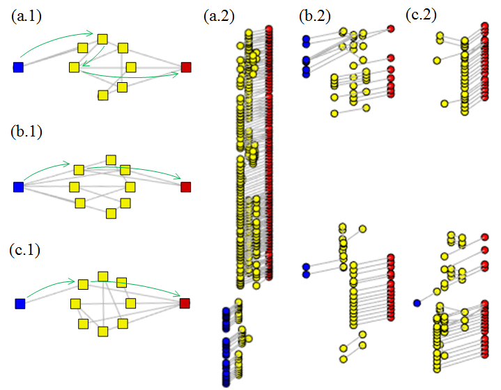
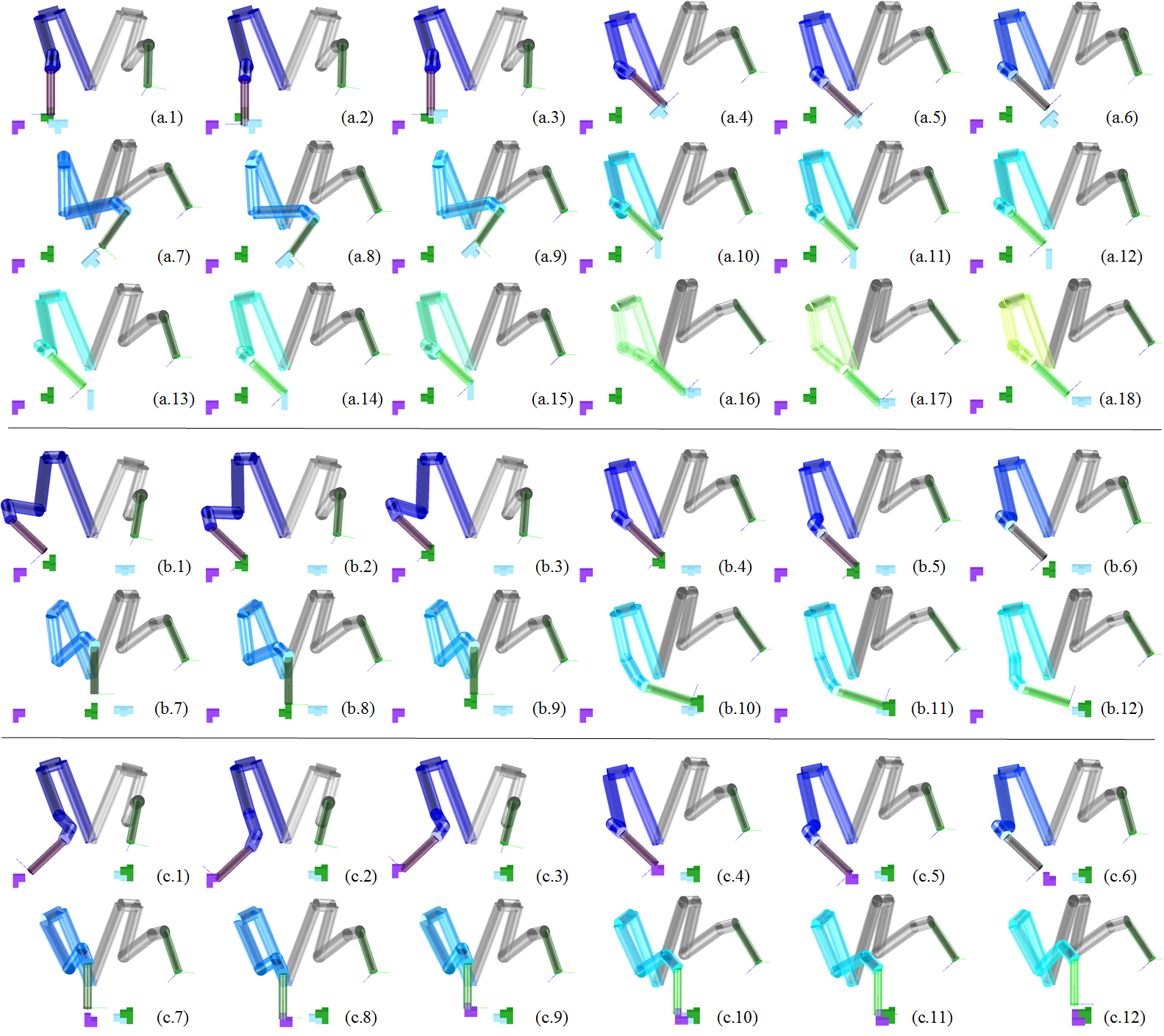
Then, the placement planner computes the stable placements for the object and the regrasp solver uses the stable placements to build a regrasp graph. The regraspgraphs are built for each object and are shown in Fig.16. Fig.16(a.1) and (a.2) are the first layer and second layer of the regrasp graph for the first object. Fig.16(b.1) and (b.2) are the first layer and second layer of the regrasp graph for the second object. Fig.16(c.1) and (c.2) are the first layer and second layer of the regrasp graph for the third object. The regrasp solver searches the regrasp graphs to find regrasp sequences. The output path on the first layers are marked using green arrows in Fig.16(a.1), (b.1), and (c.1), which implies packing the first object and the third object can be done directly, whereas packing the second object requires one time of regrasp. The sequence of robot poses and grasp configurations for the three objects are shown in Fig.17. The initial and goal poses of the objects are shown in Fig.17(a.1) and (c.6). The sequence (a.1), (a,2), …, (a.6) is to pack the first object. Fig.17(a.2) $\rightarrow$ (a.5) corresponds to the green arrow in Fig.16(a.1). The remaining poses and configurations in Fig.17(a.1), (a.3), (a.4), and (a.6) are the extended primitives. The sequence Fig.17(b.1), (b,2), …, (b.12) is to pack the second object. Fig.17(b.2) $\rightarrow$ (b.5)(b.8) $\rightarrow$ (b.11) corresponds to the green arrows in Fig.16(b.1). The remaining poses and configurations Fig.17(b.1), (b.3), (b.4), (b.6), (b.7), (b.9), (b.10), and (b.12) are the extended primitives. The sequence Fig.17(c.1), (c.2), …, (c.6) is to pack the third objects where Fig.17(c.2) $\rightarrow$ (c.5) corresponds to the green arrow in Fig.16(c.1). The remaining robot poses and grasp configurations in Fig.17(c.1), (c.3), (c.4), and (c.6) are the extended primitives.

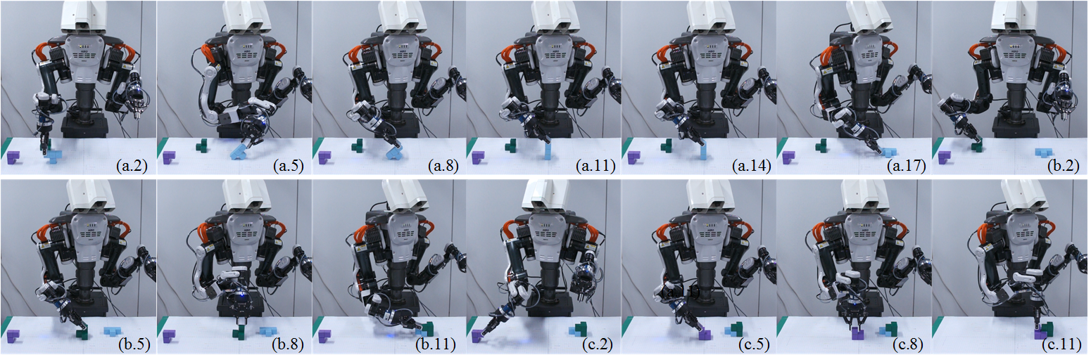
The planned results are sent to the Kawada Nextage robot for execution. Fig.18 shows the results of execution. The identifiers (a.2), (a.5), …are not continuous. They are used to help users find the correspondent robot poses and grasp configurations in Fig.17.

V-B Assembly

The mesh models used in the assembly task are shown in Fig.19. The goal is to assembly three blocks into a structure shown in the lower part of Fig.19(a). A high level planning component computes an assembly sequence which will be sent to the mid-level planning system as input. The assembly sequence includes the assembly order, assembly directions, and goal poses of the objects (Fig.19(a)). The mid-level planner uses the assembly sequence to compute the manipulation sequence of each object.

The first step is to compute the accessible grasps. Fig.19(b) shows the accessible grasps of each object following the assembly sequence in Fig.19(a). The accessible grasps are computed by the grasp planner of the mid-level planning system. Since the assembled parts become obstacles of the remaining parts, the number of accessible grasps decrease as assembly progresses.

Then, the placement planner computes the stable placements of each object and the regrasp solver uses the stable placements and their accessible grasps to build regrasp graphs. Fig.20 shows the regrasp graphs. Like Fig.16, (a.1) and (a.2) are the first layer and second layer of the regrasp graph for the first object. (b.1) and (b.2) are the first layer and second layer of the regrasp graph for the second object. (c.1) and (c.2) are the first layer and second layer of the regrasp graph for the third object. The green arrows show the paths obtained by searching the first layer. The first object requires two times of regrasp. The second and third objects both require one time of regrasp. Fig.21 shows the robot poses and grasp configurations planned by the mid-level planning system. The green arrows in Fig.20(a.1) correspond to Fig.21(a.2) $\rightarrow$ (a.5)(a.8) $\rightarrow$ (a.11)(a.14) $\rightarrow$ (a.17). The green arrows in Fig.20(b.1) correspond to Fig.21(b.2) $\rightarrow$ (b.5)(b.8) $\rightarrow$ (b.11). The green arrows in Fig.20(c.1) correspond to Fig.21(c.2) $\rightarrow$ (c.5)(c.8) $\rightarrow$ (c.11). The remaining robot poses and grasp configurations are the motion primitives.

Note that in assembly planning, the $backward$ directions of placing-down motion primitives are decided by the assembly directions planned by the high level component. This is different from packing where $backward$ is defined as the $upward$ direction. The Tool Point Center (TCP) of the active arm in the motion primitives of Fig.17(a.4) $\rightarrow$ (a.5), (a.10) $\rightarrow$ (a.11), (b.4) $\rightarrow$ (b.5), and (c.4) $\rightarrow$ (c.5) moves downwards. In contrast, the TCP of the active arm in the motion primitives Fig.21(a.16) $\rightarrow$ (a.17), (b.10) $\rightarrow$ (b.11), and (c.10) $\rightarrow$ (c.11) moves along the planned directions shown in Fig.19(a).

Like the packing task, the planned results are sent to the Kawada Nextage robot for execution. Fig.22 shows the results of execution. The identifiers (a.2), (a.5), …relate the real-world snapshots to robot poses and grasp configurations in Fig.17.

V-C Using tools

The tool used in this experiment is a drill and the robot is expected to move the drill to fasten a nut. A high-level planner specifies the goal pose of the drill and the mid-level planning system computes a sequence of robot poses and grasp configurations that move the drill from its initial pose to the goal. Fig.23 shows the regrasp graph of the drill and the simulation result. The initial and goal poses of the drill are shown in Fig.23(a) and (k). The output of the graph search in the first layer is (b) $\rightarrow$ (c) $\rightarrow$ (h) $\rightarrow$ (k). After expansion, the output is (a) $\rightarrow$ (b) $\rightarrow$ … $\rightarrow$ (k) as shown in the figure.

Fig.24 shows the results of real-world execution. The identifiers (a.2), (a.5), …relate the real-world snapshots to robot poses and grasp configurations in Fig.17.

V-D Cost analysis

The time cost of the three experiments are shown in Table.I. The values are obtained by running the algorithms on the Thinkpad P70 mobile workstation using Matlab 2016a. The operating system is Windows 10.

The columns named “Grasps”, “Placements”, and “Regrasp grasph solver” show the cost of the three planners in the mid-level planning system, respectively. The cells filled with “-” indicate their values are the same as the cells on top of them. The “IK,CD(init)”, “IK,CD(regrasp)”, and “IK,CD(goal)” under the “Regrasp grasph solver” column show the cost to compute the feasibility of IK and check the collision between the robot and obstacles at the initial object configurations, the goal object configurations, and the regrasp positions, respectively. Both original pose and the poses at the motion primitives are examined. The “IK,CD(total)” column is the sum of the values in “IK,CD(init)”, “IK,CD(regrasp)”, and “IK,CD(goal)”. The “Graph search” column shows the cost to build the two layer regrasp graph, search the graph, and generate a sequence of robot poses and grasp configurations by expanding motion primitives. It is essentially the cost of the algorithm shown in Alg.1.

The overall cost of all planners is around 300 $s$ , which implies that the algorithms cannot be used online. However, some of the data could be pre-computed offline and reused during execution. These data are marked with gray color. The grasps, the placements, and the IK and CD at the regrasp positions and goal object configurations are usually pre-defined. They can be pre-computed offline. The IK and CD at the initial object configurations must be done online since the initial object configurations are obtained from vision systems and change from time to time. The distribution of on-line and off-line computation load depends on users. Higher on-line load makes the system more flexible. For instance, making the IK and CD at the regrasp configuration online allows users to change the positions to do regrasp during execution. However, the on-line cost increases. Lower on-line load, in the extreme case, reduces time cost to less than 30 $s$ (the “IK,CD(init)” column plus the “Graph search” column) which can be used online.

TABLE I: Time efficiency of the three experiments

		Grasps	Placements	Regrasp graph solver
		Grasps	Placements	IK,CD(init)	IK,CD(regrasp)	IK,CD(goal)	IK,CD(total)	Graph search
Packing	1st object	16.865205 $s$	108.958532 $s$	8.671939 $s$	100.330880 $s$	31.503069 $s$	142.877699 $s$	2.371811 $s$
	2nd object	-	-	9.024444 $s$	-	9.836328 $s$	116.819841 $s$	0.547989 $s$
	3rd object	-	-	40.426119 $s$	-	9.733597 $s$	150.490596 $s$	0.606657 $s$
Assembly	1st object	16.139938 $s$	159.130246 $s$	11.199010 $s$	171.522333 $s$	5.736903 $s$	189.249336 $s$	0.874507 $s$
	2nd object	17.385174 $s$	104.939474 $s$	8.990426 $s$	70.594335 $s$	3.016662 $s$	82.601423 $s$	0.496157 $s$
	3rd object	16.984532 $s$	104.457831 $s$	18.872237 $s$	80.420244 $s$	1.561027 $s$	100.853488 $s$	0.448476 $s$
Using a tool	tool object	33.855902 $s$	131.262263 $s$	62.269052 $s$	108.614137 $s$	93.858813 $s$	264.742002 $s$	0.492925 $s$

VI Conclusions and Future Work

A mid-level planning system is presented in this paper. The input to the system is a sequence of object poses planned by a high-level assembly or symbolic planning component. The output of the system is a sequence of robot poses and grasp configurations that will be used by a low-level motion planning component. The planning system is composed of a grasp planner, a placements planner, and a regrasp sequence solver. The paper presented the details of these planners and solvers, and demonstrated their efficacy using three exemplary tasks.

The current implementation of the demonstrations orchestrate the planned robot poses and grasps using hard-coded interpolations. The applications are limited to small-scale wooden blocks. In the future, the mid-level planning system with be integrated with high-level and low-level components to challenge more pragmatic tasks.

Acknowledgment

This paper is based on results obtained from a project commissioned by the New Energy and Industrial Technology Development Organization (NEDO).

References

[1] L. H. de Mello, “AND/OR Graph Representation of Assembly Plans,” IEEE Transaction on Robotics and Automation, 1990.
[2] A. C. S. LS Hommem De Mello, “A Correct and Complete Algorithm for the Generation of Mechanical Assembly Sequences,” IEEE Transactions on Robotics and Automation, 1991.
[3] R. Wilson and J.-C. Latombe, “Geometric Reasoning About Mechanical Assembly,” Artificial Intelligence, 1994.
[4] M. Ghallab et al., “PDDL – The Planning Domain Definition Language – Version 1.2,” Yale Center for Computational Vision and Control, Tech. Rep., 1998.
[5] J. Hoffmann, S. Edelkamp, S. Thiebaux, R. Englert, F. dos Santos Liporace, and S. Trug, “Engineering Benchmarks for Planning: the Domains Used in the Deterministic Part of IPC-4,” Journal of Artificial Intelligence Research, 2006.
[6] L. Kavraki, P. Svestka, J. C. Latombe, and M. Overmars, “Probabilistic Roadmaps for Path Planning in High-Dimensional Configuration Spaces,” IEEE Transactions on Robotics and Automation, vol. 12, pp. 566–580, 1996.
[7] S. M. Lavalle and J. J. Kuffner, “Rapidly-Exploring Random Trees: Progress and Prospects,” in Proceedings of International Workshop on the Algorithmic Foundations of Robotics, 2000, pp. 293–308.
[8] M. Zucker, N. Ratliff, A. D. Dragan, M. Pivtoraiko, M. Klingensmith, C. M. Dellin, J. A. Bagnell, and S. S. Srinivasa, “CHOMP: Covariant Hamiltonian Optimization for Motion Planning,” International Journal of Robotic Research (IJRR), 2012.
[9] J. Schulman, Y. Duan, J. Ho, A. Lee, I. Awwal, H. Bradlow, J. Pan, S. Patil, K. Goldberg, and P. Abbeel, “Motion Planning with Sequential Convex Optimization and Convex Collision Checking,” International Journal of Robotic Research (IJRR), 2014.
[10] R. E. Fikes and N. J. Nilsson, “STRIPS: A New Approach to the Application of Theorem Proving to Problem Solving,” Artificial Intelligence, 1971.
[11] C. Belta, A. Bicchi, M. Egerstedt, E. Frazzoli, E. Klavins, and G. J. Pappas, “Symbolic Plannign and Control of Robot Motion,” IEEE Robotics and Automation Magzine, 2007.
[12] M. Lahijanian, M. R. Maly, D. Fried, L. E. Kavraki, H. Kress-Gazit, and M. Y. Vardi, “Iterative Temporal Planning in Uncertain Environments with Partial Satisfaction Guarantees,” Transaction on Robotics, 2016.
[13] M. Guo and D. V. Dimarogonas, “Multi-agent Plan Reconfiguration under Local LTL Specifications,” International Journal of Robotics Research, 2014.
[14] H. Kress-Gazit, G. E. Fainekos, and G. J. Pappas, “Temporal Logic-based Reactive Mission and Motion Planning,” IEEE Transaction on Robotics, 2009.
[15] A. Hertle, “Design and Implementation of an Object-Oriented Planning Lanuage,” Master’s thesis, Albert-Ludwigs-Universitat reiburg, 2011.
[16] M. Dogar, A. Spielberg, S. Baker, and D. Rus, “Multi-Robot Grasp Planning for Sequential Assembly Operations,” in Proceedings of IEEE International Conferene on Robotics and Automation (ICRA), 2015.
[17] J. Bidot, L. Karlsson, F. Lagriffoul, and A. Saffiotti, “Geometric Backtracking for Combined Task and Motion Planning in Robotic systems,” Artificial Intelligence, 2015.
[18] R. Knepper, T. Layton, J. Romanishin, and D. Rus, “IkeaBot: An Autonomous Multi-robot Coordinated Furniture Assembly System,” in Proceedings of IEEE International Conference on Robotics and Automation (ICRA), 2013.
[19] D. Stein, T. R. Schoen, and D. Rus, “Constraint-aware Coordinated Construction of Generic Structures,” in Proceedings of IEEE International Conference on Intelligent Robots and Systems, 2011.
[20] R. Knepper and D. Rus, “Pedestrian-inspired Sampling-based Multi-robot Collision Avoidance,” in Proceedings of IEEE International Symposium on Robot and Human Interactive Communication, 2012.
[21] L. P. Kaelbling and T. Lozano-Perez, “Integrated Task and Motion Planning in Belief Sapce,” International Journal of Robotics Research, 2013.
[22] N. T. Dantam, “The Motion Grammar: Analysis of a Linguistic Method for Robot Control,” IEEE Transactions on Robotics, 2013.
[23] K. Hauser and J.-C. Latombe, “Multi-modal Motion Planning in Non-expansive Spaces,” International Journal of Robotics Research, pp. 897–915, 2010.
[24] N. Dantam, Z. Kingston, and S. Chauhuri, “Incremental Task and Motion Planning: A Constraint-Based Approach,” in Proceedings of Robotics: Science and Systems (RSS), 2016.
[25] A. Krontiris and K. Bekris, “Efficiently Solving General Rearrangement Tasks: A Fast Extension Primitive For An Incremental Sampling Based Planner,” in Proceedings of IEEE International Conference on Robotics and Automation (ICRA), 2016.
[26] S. Nedunuri, S. Prabhu, and M. Moll, “SMT-based Synthesis of Integrated Task and Motion Plans from Plan Outlines,” in Proceedings of IEEE International Conference on Robotics and Automation (ICRA), 2014.
[27] J. King, M. Klingensmith, and C. Dellin, “Regrasp Manipulation as Trajectory Optimization,” in Proceedings of Robotics: Science and Systems (RSS), 2013.
[28] F. W. Heger, “Assembly Planning in Constrained Environments: Building Structures with Multiple Mobile Robots,” Ph.D. dissertation, Carnegie Mellon University, 2010.
[29] E. Yoshida, C. Esteves, O. Kanoun, M. Poirier, A. Mallet, J.-P. Laumond, and K. Yokoi, “Planning Whole-body Humanoid Locomotion, Reaching and Manipulation,” Motion Planning for Humanoid Robots, pp. 99–128, 2010.
[30] P. Tournassound, T. Lozano-Perez, and E. Mazer, “Regrasping,” in Proceedings of International Conference on Robotics and Automation, 1987, pp. 1924–1928.
[31] F. Rohrdanz and F. M. Wahl, “Generating and Evaluating Regrasp Operations,” in Proceedings of International Conference on Robotics and Automation, 1997, pp. 2013–2018.
[32] S. A. Stoeter, S. Voss, N. P. Papanikolopoulos, and H. Mosemann, “Planning of Regrasp Operations,” in Proc. of ICRA, 1999, pp. 245–250.
[33] H. Terasaki and T. Hasegawa, “Motion Planning of Intelligent Manipulation by a Parallel Two-Fingered Gripper Equiped with a Simple Rotating Mechanism,” IEEE Transaction on Robotics and Automation, 1998.
[34] K. Cho, M. Kim, and J.-B. Song, “Complete and Rapid Regrasp Planning with Look-up Table,” Journal of Intelligent and Robotic Systems, pp. 371–387, 2003.
[35] D. R. Rapela and U. Rembold, “Planning of Regrasping Operations for a Dexterous Hand in Assembly Tasks,” Journal of Intelligent and Robotic Systems, vol. 33, pp. 231–266, 2002.
[36] Z. Xue et al., “Planning Regrasp Operations For A Multifingered Robotic Hand,” in Proceedings of International Conference on Automation Sicence and Engineering, 2008, pp. 778–783.
[37] P. Lertkultanon and Q.-C. Pham, “A single-query manipulation planner,” 2016.
[38] Y. Koga and J.-C. Latombe, “Experiments in Dual-arm Manipulation Planning,” in Proceedings of IEEE International Conference on Robotics and Automation (ICRA), 1992, pp. 2238–2245.
[39] ——, “On Multi-Arm Manipulation Planning,” in Proceedings of IEEE International Conference on Robotics and Automation (ICRA), 1994, pp. 945–952.
[40] N. Vahrenkamp, D. Berenson, T. Asfour, J. Kuffner, and R. Dillmann, “Humanoid Motion Planning for Dual-arm Manipulation and Regrasp Tasks,” in Proceedings of IEEE/RSJ International Conference on Intelligent Robots and Systems (IROS), 2009.
[41] B. Cohen et al., “Planning Single-arm Manipulations with N-Arm Robots,” in Proceedings of Robotics: Science and Systems, 2010.
[42] K. Harada et al., “Project on development of a robot system for random picking-grasp/manipulation planner for a dual-arm manipulator,” in IEEE/SICE International Symposium on System Integration (SII), 2014, pp. 583–589.
[43] W. Wan, M. T. Mason, R. Fukui, and Y. Kuniyoshi, “Improving regrasp algorithms to analyze the utility of work surfaces in a workcell,” in Proceedings of International Conference on Robotics and Automation, 2015.
[44] W. Wan and K. Harada, “Reorientating Objects with a Gripping Hand and a Table Surface,” in Proceedings of international Conference on Humanoid Robots, 2015.
[45] C. Cao, W. Wan, J. Pan, and K. Harada, “Analyzing the Utility of a Support Pin in Sequential Robotic Manipulation,” in Proceedings of IEEE International Conference on Robotics and Automation (ICRA), 2016.
[46] J.-P. Saut, M. Gharbi, J. Cortes, D. Sidobre, and T. Simeon, “Planning Pick-and-place Tasks with Two-hand Regrasping,” in Proceedings of IEEE/RSJ International Conference on Intelligent Robots and Sytems (IROS), 2010.
[47] W. Wan and K. Harada, “Developing and Comparing Single-arm and Dual-arm Regrasp,” IEEE Robotics and Automation Letters, 2016.
[48] ——, “Achieving High Success Rate in Dual-arm Handover Using Large Number of Candidate Grasps,” Advanced Robotics, 2016.
[49] K. K. Hauser, T. Bretl, K. Harada, and J.-C. Latombe, “Using Motion Primitives in Probabilistic Sample-Based Planning for Humanoid Robots,” in Proceedings of Robotics: Science and Systems (RSS), 2006.
[50] X. Ding and C. Fang, “A Novel Method of Motion Plnning for an Anthropomorphic Arm Based on Movement Primitives,” IEEE Transactions on Mechatronics, 2013.
[51] D. Hsu, T. Jiang, J. Reif, and Z. Sun, “The Bridge Test for Sampling Narrow Passages with Probabilistic Roadmap Planners,” in Proceedings of IEEE International Conference on Robotics and Automation (ICRA), 2003.
[52] A. Yershova and S. M. LaValle, “Motion Planning for Highly Constrained Spaces,” in Robot Motion and Control 2009. Springer, 2009, pp. 297–306.

A Mid-level Planning System for Object Reorientation