Cellular Legendrian contact homology for surfaces, part IIThanks: We thank Tobias Ekholm for explaining his transversality argument. The second author is supported by grant 317469 from the Simons Foundation. He thanks the Centre de Recherches Mathematiques for hosting him while some of this work was done.
Abstract.
This article is a continuation of [15]. For Legendrian surfaces in -jet spaces, we prove that the Cellular DGA defined in [15] is stable tame isomorphic to the Legendrian contact homology DGA.
1. Introduction
This article is a continuation of [15]. Together the two articles provide a formulaic computation of the Legendrian contact homology (LCH) differential graded algebra (DGA) for any Legendrian surface in a -jet space. In [15] we compute the LCH DGA for several families of examples, and in [16] we apply our results to study augmentations and generating families.
Let be a surface, and let be a closed Legendrian surface in the -jet space of In [15], we defined the cellular DGA of , denoted here as . The definition of requires as input a cellular decomposition of the base projection of that contains in its -skeleton the projection of all crossings arcs, cusp edges, and swallowtail points from the front projection. For each cell, we have one generator of for each pair of sheets above the cell that and do not cross one another. After collecting generators into upper triangular matrices, the differential is characterized by simple matrix formulas as summarized in Figure 1. (Additional terms appear when swallowtail points are present.)
We have established in Theorem 4.1 of [15] that is determined, up to stable tame isomorphism, by the Legendrian , i.e., it does not depend on the cellular decomposition or other choices involved in the definition. In the present article, we prove the following:
Theorem 1.1.
Let be a closed Legendrian surface. The cellular DGA of is stable tame isomorphic to the Legendrian contact homology DGA of with coefficients in .
In particular, the cellular DGA is an invariant of the Legendrian isotopy class of . We remark that it would be interesting to have an independent, low-tech proof of invariance that skirts the theory of holomorphic curves.
1.0.1. Outline of proof
The proof of Theorem 1.1 occupies this entire article, and we now provide an outline of the argument. In this introduction, we denote the LCH DGA as .
Our starting point is the work of Ekholm [4] that allows the differential in , that was originally defined in [6] and [8] by a count of holomorphic disks, to be computed via a count of rigid gradient flow trees (abbrv. GFTs). In Section 2, we recall relevant background about the LCH DGA and GFTs. In Section 3, we construct a cellular decomposition of into squares, , so that, in the front projection of , the form of the singular set above each square matches one of 14 standard types. (See Figure 4, below.) In addition, we construct a related cellular decomposition, , that is suitable from the point of view of the cellular DGA.
For computing LCH, we modify by a Legendrian isotopy to a Legendrian that has several properties that aid in the explicit enumeration of rigid GFTs. Most importantly, the sheets of are pinched together above the -skeleton of with the pinching most exaggerated above the -skeleton. As a result, above each cell of dimension , each pair of sheets are connected by a Reeb chord that when viewed as a critical point of the difference of -coordinates of sheets has index . (Some additional Reeb chords that we call exceptional generators appear as well and are discussed below.) Labeling Reeb chords between the -th and -th sheet above -cells, -cells, and -cells in the form , , and , gives a rough indication of the correspondence between generators of and underlying the isomorphism of Theorem 1.1. See Figure 1. As an additional consequence of the pinching near the -skeleton, the GFTs used in computing the differential of become localized and must remain entirely within a neighborhood of the square that they begin in. The Reeb chords that appear above suitable neighborhoods of any closed cell from then generate a sub-DGA, so that computation of may be carried out on a square-by-square basis.
at 170 192 \pinlabel [b] at 170 350 \pinlabel [r] at 0 232 \pinlabel [l] at 328 232 \pinlabel [t] at 170 20 \pinlabel [l] at 328 330 \pinlabel [l] at 328 36 \pinlabel [r] at 0 330 \pinlabel [r] at 0 36 \pinlabel [l] at 640 240 \pinlabel [l] at 820 240 \pinlabel [bl] at 504 46 \endlabellist

; ;
.
The enumerations of GFTs required for computation of the sub-DGAs corresponding to individual cells of are carried out in Sections 5-7. A common argument applies for all squares that do not contain swallowtail points. To orient the reader for this general computation, the logically independent Section 4 outlines in detail the computation for two of the most basic square types with technical details simplified or ignored. In Section 5, we compute the sub-DGAs associated to -cells and -cells. In Section 6, we compute in a uniform manner the sub-DGAs of all -cells that do not contain swallowtail points. In Section 7, we address squares with swallowtail points.
To be more precise, in Sections 5-7 we only give a partial calculation of the differential in . The reason for this is that the presence of crossing arcs above a square forces additional Reeb chords that we call exceptional generators to appear. In turn, these exceptional generators lead to GFTs that can be quite complicated, so that a complete calculation would require special arguments for many of the different square types. To keep the computation as uniform as possible, in Sections 5-7 we only compute up to terms belonging to an ideal involving these exceptional generators. Aside from these terms, for each of the first 12 square types the differential is given by a common matrix formula where certain matrix entries are replaced with ’s and ’s in a way that is determined by the location of crossing arcs and cusp edges. The final two square types contain swallow tail points, and as a result differentials in these square types have a form that is genuinely distinct from the other twelve square types.
To avoid having to explicitly identify the remaining terms involving exceptional generators, we show in the first half of Section 8, that the quotient of by the differential ideal is stable tame isomorphic to . Moreover, our partial calculations from Sections 5-7 give a complete calculation of the differential in . Section 8 is then concluded by establishing Theorem 1.1 via a stable tame isomorphism between and the cellular DGA.
The final Sections 9-12 give a rather explicit coordinate model for that is used for the calculation of in the earlier sections of the paper. This construction is technical (although elementary). To allow the reader to understand the computation of LCH without worrying about the details of this coordinate construction, we have listed those properties of that are required for the arguments as Properties 1-19 appearing in Sections 5-7. We expect that most readers will not find it surprising that a Legendrian satisfying Properties 1-19 exists. However, as many properties involving the critical points and gradient vector fields of local defining functions for and their difference functions are demanded simultaneously, we did not feel that the existence of was entirely obvious. An outline of the construction appears at the start of Section 9.
1.0.2. Strategies for reading.
For a first reading, the details of the construction from Section 9-12 may be omitted. The reader may also reduce the length of the proof by considering only the case of Legendrians without swallowtail points. This eliminates Sections 7 and 10, and simplifies the isomorphism in Section 8 as well as parts of Section 11. In fact, for some purposes considering only Legendrian surfaces without swallowtail points may suffice. By work of Entov [11, Corollary 1.8 and Section 1.8], assuming the base surface and Legendrian are orientable, it is always possible to remove all swallowtail points from via a Legendrian isotopy. However, in practice, it can be difficult to explicitly find such an isotopy for a given Legendrian, and the number of generators of the cellular DGA may be greatly increased by removing swallowtail points. Thus, aside from removing any assumptions on the orientability of and , the extra work involved to include swallow tail points is justified in order to make the cellular DGA a flexible tool for computations. For example, a configuration of four swallowtail points can collapse to a cone point, whose DGA we compute in Section 5.3 of [15], and the cone points appear in the work-in-progress by Casals and Murphy on Lefschetz fibrations.
2. Background
We assume familiarity with [15, Sections 2 and 3]. In particular, the reader should be familiar with the generic appearance of the base and front projection of a Legendrian surface in a -jet space; the latter may include cusp edges, crossing arcs, and (upward and downward) swallowtail points. We refer to this subset of the front projection (cusp edges, crossing arcs and swallowtail points) and sometimes its base projection as the singular set. The definition of the cellular DGA from [15, Section 3] as well as algebraic results on DGAs (differential graded algebras) and stable tame isomorphism as found in [15, Section 2] are required for the proof of Theorem 1.1. In this section, we recall background on Legendrian contact homology, focusing on Ekholm’s work on gradient flow trees which is fundamental for this article.
Let be a surface. Denote the -jet space of as . Define the front projection the base projection and the Lagrangian projection In coordinates arising from a choice of local coordinates on , the standard contact structure on is the kernel of the contact form Let be the standard symplectic structure on where locally
2.1. LCH
Let be a Legendrian surface. The Legendrian contact homology (LCH) of is the homology of a differential graded algebra (DGA) denoted whose definition is based on the theory of -holomorphic curves. The LCH DGA was first introduced in [10] and was then rigorously defined in [6, 8]. In reviewing the definition, it is natural to use -coefficients and introduce a -grading on , but in the remainder of the article we will specialize to coefficients in (all group ring generators are replaced with ) and collapse the grading modulo the Maslov number of .
2.1.1. Reeb chords and the algebra
The Reeb vector field associated to a contact form is defined as the unique vector field which satisfies and For our contact form on , the Reeb vector field is The Reeb chords for our Legendrian are the (non-constant) flows lines of the Reeb vector field that begin and end on the Legendrian.
Assuming that has a generic front projection, we can write where has codimension and the front projection satisfies:
- •
is an immersion when restricted to ;
- •
has a cusp edge singularity along ;
- •
has (upward or downward) swallowtail singularities at points in .
Any has a neighborhood that is the -jet of a function . We say that is a local defining function for at . The Reeb chords are in one-to-one correspondence with the critical points of positive critical value, where and are two such local defining functions for [The critical points are in the intersection of the domains of and ] As an additional generic assumption on the front projection of , we assume that the critical points of the are Morse.
The restriction of to is an exact Lagrangian immersion. Reeb chords are also in one-to-one correspondence with the double points of , which are transverse due to the previous assumption on the .
The underlying algebra of the LCH DGA is defined to be the free unital associative (non-commutative) over the group ring with generating set . This is the tensor algebra of the -module generated by
2.1.2. The grading on
We review the (Maslov) grading of a Reeb chord and the (minimal) Maslov number of the Legendrian, as formulated in [7, Section 3]. Let be such that except for at isolated points where intersects transversely. Define (resp. ) to be the number of intersections of with where (oriented by ) goes from the upper (resp. lower) sheet to the the lower (resp. upper) sheet of the pair of cusping sheets. Let Define the Maslov number of to be the minimum non-negative integer value achieved by over all loops
Denote the connected components of as , and choose base points . Given a Reeb chord , let where has the greater -coordinate of the two. Supposing that and , we choose generic base point paths such that , , and , and let which is a single oriented path from to when and a disjoint union of oriented paths when . Define the grading of by
| (1) |
where and are local defining functions for the sheets containing and respectively, and denotes the Morse index of as a critical point of .
We extend the grading of Reeb chords to a grading of as a direct sum of -modules, , by requiring that for a homology class , has and that holds when and are homogeneous elements.
Remark 2.1.
For Legendrian isotopy invariance of in the multiple component case where , we need to allow for an overall grading change determined by a choice of integers . Given , we obtain an alternate grading of Reeb chords by replacing each with when has lower endpoint on and upper endpoint on .
Alternatively, a grading of Reeb chords by may be defined without reference to base point paths as follows. Fix a choice of Maslov potential, i.e. a locally constant function whose value increases by when passing from the lower sheet to the upper sheet at cusp edges. Then,
| (2) |
Note that when is connected, the grading is independent of the choice of Maslov potential and is the reduction of the grading from (1) mod . In the multi-component case, gradings resulting from different Maslov potentials are related to one another and to the grading from (1) as in Remark 2.1.
2.1.3. The LCH differential
For any non-negative integer let be the space of closed unit disks in centered on the origin, with punctures removed from the boundary in counter-clockwise order such that (if exist). Let be the set of -tame almost complex structures with equality holding if and only if As a technical condition, we also need to assume for there exists some neighborhood of the double points in where looks like the standard complex structure of [8, page 3305]. Let and let denote the complex structure on any inherited from Fix with base point paths Fix an element For let be the moduli space of equivalence class of pairs such that the following hold.
- •
The pair is comprised of and
- •
The image under of a sequence of points converging to the puncture (resp. ) converges to the double point (resp. ). Moreover, the image of near (resp. ) in the positive (resp. negative) oriented boundary direction runs from the branch (of the two branches that intersect at the double point (resp. )) of with the lower -coordinate lift in to the branch with the higher -coordinate lift.
- •
Combining the continuous lift of in with the base point paths and produces a representative for
- •
The map restricted to the interior of is -holomorphic,
- •
Two pairs and are equivalent if there exists a biholomorphic map of the unit disk taking the punctures of to those of such that
Define the formal dimension of the moduli space to be
For any such that there exists an open dense subset such that is a manifold, compact in the sense of Gromov (see [6], for example) whose dimension equals its formal dimension [8]. So for is a finite set of points when , cf. [6, 8].
We can now define the differential . For Reeb chords , set
and then extend to all of with the (-linear) Leibniz rule. Here is a -count. If then the empty word is
Theorem 2.2 ([6, 8]).
The differential has degree and satisfies Moreover, if and are Legendrian isotopic, then for any , and any choice of base point paths, the DGAs and are stable tame isomorphic (after possibly applying a grading change as in Remark 2.1).
In particular, the homology called the Legendrian contact homology, is a well-defined Legendrian isotopy invariant.
2.2. Gradient flow trees
In [4], Ekholm showed that the count of homolorphic disks appearing in the definition of LCH may be replaced with a count of suitable gradient flow trees (abbrv. GFTs). This is a significant extension of earlier results of Floer [12] and Fukaya-Oh [13] that relate holomorphic strips and disks to gradient trajectories and flow trees in the case of graphical Legendrians. In this article, we only consider GFTs with a single positive puncture. This allows a definition of GFT that appears somewhat different from the general definition given in [4], but more closely parallels the presentation of flow trees from [13]. See Remark 2.5.
We consider rooted trees, i.e. trees with a finite number of edges and with a chosen -valent initial vertex, (For those familiar with [4], we recast -valent initial vertices as discussed later in Remark 2.8.) We orient the edges of a rooted tree so that all edges are oriented away from . Note that any other vertex has precisely one incoming edge that is oriented towards while any other adjacent edges are oriented away from . Vertices with valence (resp. valence greater than ) are called external (resp. internal). Sometimes, we refer to as the input vertex, and to the remaining external vertices as output vertices. Edges with both endpoints at internal vertices are internal, while edges with at least one endpoint at an external vertex are external.
A metric tree with input is a rooted tree equipped with the following additional structure:
- (1)
Each edge is assigned a length such that (i) all internal edges have finite length, and (ii) the initial edge that starts at has length .
- (2)
At each internal vertex an ordering of the outgoing edges is chosen.
To each edge, , of a metric tree, we assign an interval according to:
- •
The initial edge beginning at has unless it is the only edge of in which case .
- •
All other edges, , have .
Fix a Riemannian metric on .
Definition 2.3.
A gradient flow tree (abbrv. GFT) of (with respect to the metric ) is a metric tree together with for each edge a continuous map
together with a pair of -jet lifts
satisfying:
- (1)
For all, .
- (2)
For all , where and are local defining functions for at and , respectively.
- (3)
If is an internal edge, then is non-constant.
- (4)
At each internal vertex, , write the edges adjacent to as , , where is the unique edge oriented into and are the outgoing edges at appearing according to their order. Notate corresponding edge maps as , . We require that the -jet lifts fit together continuously at as follows
(See Figure 2.)
- (5)
The initial edge, , that begins at , satisfies where the Reeb chord is a critical point of .
- (6)
An external vertex at the end of an edge , we either have
- (a)
and where the Reeb chord is a critical point of , or
- (b)
the images agree and belong to a cusp edge of .
- (a)
A partial flow tree (abbrv. PFT) is a rooted tree satisfying all of the properties of a GFT except that the initial edge starting at is parametrized with where , and no requirement is placed on the image at other than . In particular, this input edge is no longer required to begin at a Reeb chord.
We introduce some additional terminology associated with a GFT or PFT . When the input vertex begins at the Reeb chord we say that the vertex is a positive puncture at . When an output vertex limits to a Reeb chord as , we say that is a negative puncture at . We refer to output vertices that end at a point on the cusp edge of as -vertices.
Often, we will provide a labeling of the sheets of above some subset as , and denote the corresponding local defining functions by . (We emphasize that such an enumerations of sheets of only makes sense locally.) Typically, we shorten notation for the local difference functions to
When the -jet lifts, and , of an edge of a GFT or PFT have their images in and respectively, we say that (resp. ) is the upper sheet (resp. lower sheet) of . Note that in this case is a trajectory for , and we say that is an -flow line.
Observation 2.4.
- (i)
For any point belonging to the interior of one of the edges of a GFT or PFT , there is a unique PFT whose initial vertex is that consists of the portion of that lies below (with respect to the orientation of edges of the domain tree of ). Usually, we refer to this PFT as simply the PFT starting with .
- (ii)
External edges may be mapped to Reeb chords as constant maps. In fact this must be the case for GFTs that have a positive (resp. negative) puncture at a Reeb chord that is a local minimum (resp. maximum) of .
- (iii)
The sheet difference decreases not only along every non-constant edge (as a standard consequence of the negative gradient flow equation), but also when passing internal vertices (from the incoming edge to an outgoing edge). Thus, if and are any points in the domain of a PFT with above (with respect to the orientation of edges of ), then the sheet difference at is larger than at .
Remark 2.5.
- (i.)
Our definition of PFT is much more restrictive than in [4], where more than one exceptional vertex is allowed.
- (ii.)
In [4], the definition of GFT does not allow constant external edges (mapped to Reeb chords). However, [4] does allow punctures to occur at internal vertices, as we explicitly do not. The equivalence of these conventions is easily seen: A constant edge may be replaced with a puncture at an internal vertex in a unique way and the converse statement holds also.
- (iii.)
The condition is not included in the definition of GFT from Ekholm. Indeed, this condition may fail for GFTs with more than one positive puncture. However, Lemma 2.8 from [3], establishes this condition for GFTs with positive puncture.
2.2.1. Words of GFTs and PFTs
We define the word, , of a PFT or GFT, , using induction on the number of internal vertices. If has no internal vertices then, its domain is a single edge with one output vertex, . In this case, declare
Now, supposing has been defined for PFTs with fewer internal vertices, we consider the first internal vertex, , of . Let the outgoing edges at be ordered as , for some . Let denote the PFTs of that begin at interior points of the edges respectively, and define
An alternate formulation of is as follows: The ordering of outgoing edges at internal vertices, allows us to embed the domain tree of into by requiring that the outgoing edges at an internal vertex appear in counterclockwise order when we travel around starting at the incoming edge. Moreover, we can arrange the external vertices to sit on , and their cyclic ordering is well defined. We then take the product of all negative punctures, , as they appear in counter-clockwise order around , starting at . That is,
Yet another perspective on is the following: The union of the Lagrangian projections of the one jet lifts and (the negative indicates orientation reverse) of all edges of fit together to give a continuous closed curve, , with image in . We call the boundary curve of . See Figure 2. When instead considered as a curve on , has discontinuities that are in bijection with the positive and negative punctures of . (The -coordinate increases (resp. decreases) when passing a positive (resp. negative) puncture.) From this perspective, is the product of negative punctures as they appear along the curve , when starting with the upper lift of the initial edge of .
When is a GFT with positive puncture at and , we say that is a GFT from to .
[r] at 44 144 \pinlabel [l] at 90 144 \pinlabel [b] at 334 200 \pinlabel [t] at 254 12 \pinlabel [t] at 304 4 \pinlabel [t] at 344 -2 \pinlabel [t] at 386 4 \pinlabel [t] at 434 20 \pinlabel [b] at 72 174 \pinlabel [t] at -2 30 \pinlabel [t] at 72 36 \pinlabel [t] at 146 30 \endlabellist

2.3. GFTs and Holomorphic Disks
The connection between GFTs and Legendrian contact homology is the following.
In Section 3 of [4], Ekholm associates a formal dimension to a GFT, , from to written, . It is equal to the formal dimension of the moduli space of holomorphic disks , where is the lift of the boundary curve of to (this is discontinuous at punctures) together with the base point paths and . The pair consisting of the Legendrian and metric is -regular when (i) there are no GFTs with , (ii) all trees with are transversally cut out (i.e. they are obtained via iterated transverse intersection of certain suitably defined ascending and descending manifolds), and (iii) the set of trees with is finite. (The “” in -regular refers to the number of positive punctures.) When is -regular, GFTs with formal dimension are called rigid.
It is shown in [4, Theorem 1.1 (a)] that any can be made -regular after a -small perturbation. For the Legendrians that we consider we will use a mild strengthening of this statement; see Proposition 12.2.
Theorem 2.6 ([4], Theorem 1.1).
Suppose that is -regular. There exists a Legendrian such that
- (1)
is Legendrian isotopic to , and has its Reeb chords canonically identified with those of , and
- (2)
there exists for such that when , disks in for are in bijection with the set of (equivalence classes of) rigid GFTs for from to whose boundary curves satisfy .
In particular, the differential in the LCH DGA of may be computed by
where the sum is over all rigid GFTs for that begin at .
2.4. Generic behavior at vertices
In Section 3 of [4], it is shown that when is -regular the internal vertices that appear in rigid GFTs are limited to the following types:
- •
A -vertex, , is a -valent vertex with image in disjoint from the cusp locus of . At , there exist sheets with defining functions satisfying , such that the incoming edge at is an -flow line while the outgoing edges and are respectively - and -flow lines.
- •
A -vertex, , is a -valent vertex with image at a point of belonging to the cusp locus of such that the sheets corresponding to edges adjacent to are as follows. Near there are sheets of such that sheets and meet at a cusp edge so that has larger -coordinate than ; sits above the cusp edge; and sits below the cusp edge. The incoming edge is an -flow line while the out going edges and are respectively - and -flow lines. In addition, and are all transverse to the cusp locus of at , and necessarilly point to the side of the cusp locus where and exist.
- •
A -vertex (also called a switch vertex), , is a -valent vertex with image at the base projection of a cusp edge where sheets and meet with the upper sheet of the cusp edge. In addition, one of the following holds:
- (i)
The incoming (resp. outgoing) edge at is an -flow line (resp. an -flow line) for some sheet that sits above the cusp edge at . Note that must be tangent to the cusp locus at .
- (ii)
The incoming (resp. outgoing) edge at is a -flow line (resp. a -flow line) for some sheet that sits below the cusp edge. Note that is tangent to the cusp locus at .
- (i)
See Figure 3.
We use the terminology switch point for a point along the projection of a cusp edge between sheets and where a third sheet or as in (i) or (ii) has or tangent to the projection of the cusp edge. A switch point is non-degenerate when the tangency of the restriction of the corresponding or to the cusp locus has order . Of course, switch vertices can only have their images at switch points.
[r] at -50 102 \pinlabel [l] at 50 126 \pinlabel [br] at 14 50 \pinlabel [bl] at 62 50 \pinlabel [l] at 388 154 \pinlabel [l] at 388 90 \pinlabel [l] at 388 26 \endlabellist

[r] at -50 102 \pinlabel [l] at 50 126 \pinlabel [br] at 14 50 \pinlabel [bl] at 62 50 \pinlabel [l] at 398 154 \pinlabel [l] at 398 108 \pinlabel [l] at 398 60 \pinlabel [l] at 398 26 \endlabellist

[r] at -60 102 \pinlabel [l] at 18 88 \pinlabel [l] at 18 44 \pinlabel [l] at 360 108 \pinlabel [l] at 360 60 \pinlabel [l] at 360 18 \endlabellist

Theorem 2.7 ([4]).
Assume is 1-regular. Then, all internal vertices of rigid GFTs must be either -, -, or -vertices. (External vertices may be punctures or -vertices.)
Proof.
In Section 3 of [4], GFTs are assigned a geometric dimension, . [4, Proposition 3.14] shows that when is transversally cut out, a space of nearby GFTs with similar geometric properties, eg. homeomorphic domain trees with corresponding branches having the same upper and lower sheet in , is a manifold of dimension . In particular, a transversally cut out tree has . Moreover, [4, Lemma 3.7] shows that in general , so that a rigid tree must have . Possible vertices of trees with are listed in [4, Lemma 3.7]. ∎
Remark 2.8.
In [4, Lemma 3.7], -valent vertices with a positive (resp. negative) puncture at a local minimum (resp. local maximum) are also listed as possible internal vertices. However, with our conventions for GFTs, such punctures become ’s with an adjacent external edge mapped to a constant trajectory at the corresponding critical point. See Remark 2.5 (ii).
Moreover, for GFTs with these generic vertices, formal dimension may be computed from the count of vertices of various types and the Morse index of punctures.
Proposition 2.9.
Suppose that is -regular. Let is a rigid GFT with a postive puncture at and negative punctures at . Let , , and denote the number of , , and -vertices of respectively, and and denote the Morse indices of and as critical points of local difference functions with . Then, we have
| (3) |
3. Transverse Square Decompositions
Let be a Legendrian with generic front projection and base projection, and let denote the singular set (cusps, crossings and swallowtails) of the front projection of . In this section, we construct a cell decomposition of into squares. The -skeleton will be transverse to , so we will denote the decomposition as . Above each square of , is required to match one of a finite collection of standard forms that are introduced in Section 3.2 below, and a few additional technical requirements are imposed on for later use. In addition, we construct a related cellular decomposition that will be used in Section 8 when working with the Cellular DGA.
3.1. Regularity requirements
We impose some regularity requirements on our square decomposition. In this section we use the notation .
For the transverse cell decomposition constructed below, we always require the following conditions. Note that these requirements may be obtained from an arbitrary polygonal decomposition (as in Section 3.1 of [15]) into squares by altering the original characteristic maps first near -cells and then in a neighborhood of -cells.
- (1)
We have characteristic maps
which are homeomorphisms and are smooth with smooth inverse except possibly at the corners of -cells. (Compare with requirement (2) below).
- (2)
Each -cell has a disk coordinate neighborhood so that if distinct -cells meet at then near the corner each of their characteristic maps rescales the angle. More precisely, for a given -cell containing as a corner, we use polar coordinates on centered at the corner of corresponding to with the angle coordinate rotated so that parametrizes a neighborhood of this corner. We require that the characteristic map for takes into and has the form
for , for some .
- (3)
Along each -cell, the characteristic maps of the -adjacent faces may be glued together to give smooth maps .
3.1.1. Where do the technical requirements come into play?
In Sections 9-12, we will define a front projection for a Legendrian that is isotopic (but not literally equal to) the original front projection of . This is done by providing local defining functions for the sheets of above each square using coordinates given by the characteristic maps. This explains (1). Near corners each local defining function will have the form in the polar coordinate system centered at the corner of as described in (2) with the coefficients and agreeing for sheets in distinct squares that meet at the -cell. Therefore, the requirements from (2) show that the front will be smooth in a neighborhood of a -cell. Moreover, the construction of sheets will be standard near edges as well, so that (3) will guarantee the smoothness of the pieced together front above -cells.
In addition, the conditions allow the following:
Construction 3.1.
Let be a Legendrian with local defining functions given by in the coordinate neighborhoods of -cells prescribed in (2). There exists a metric on with respect to which the gradients of local defining functions (and hence also local difference functions) agree with the gradients taken in each square with respect to the standard Euclidean metric on .
Proof.
The Euclidean metrics on squares piece together to give a metric on the complement of the -cells of . In a coordinate neighborhood (as in (2)) of a -cell adjacent to faces, the metric appears in polar coordinates as . In order to extend smoothly to , we alter the metric inside to where is a bump function that is outside values of where all local defining functions have the form and is in a neighborhood of .
This change to the metric does not alter gradients of functions of the form . ∎
3.2. Elementary squares
In Figure 4, some standard forms for the base projection of the crossing and cusp loci of a Legendrian to a square are presented and divided into Types (1)-(14). Note that parametrizations of squares may be orientation reversing (supposing is oriented, which we do not require in general) so that the images of the cusp and crossing locus in may appear reflected across in some squares.
For some edges of the squares of type (5), (6), (8) or (12), a pair of arcs of the crossing locus intersect a single edge. Along such an edge either the or -coordinate goes from to while the other coordinate remains fixed. Denote the coordinate that varies by . We require that the two crossings that appear along the restriction of to that edge arise from a strand with larger -coordinate at passing through two consecutive strands with lesser -coordinate at as increases. See the image labelled (2Cr) in Figure 5. Thus, when viewed with this prescribed orientation, above each edge of a square of Type (1)-(14) the singular set matches of the forms pictured in Figure 5.
We refer to a square in above which has one of the types (1)-(14) as an elementary square for .
(PV) [t] at 100 0 \pinlabel(1Cr) [t] at 370 0 \pinlabel(2Cr) [t] at 640 0 \pinlabel(Cu) [t] at 910 0 \pinlabel [l] at 468 96 \pinlabel [l] at 468 56 \pinlabel [l] at 738 96 \pinlabel [l] at 738 56 \pinlabel [l] at 738 16 \pinlabel [l] at 1008 96 \pinlabel [l] at 1008 56 \endlabellist

3.3. Requirements for the transverse square decomposition
We will want to construct a transverse square decomposition for together with a choice of orientation for each of the -cells of so that a list of conditions (A1)-(A4) is satisfied. We state (A1)-(A3) now, and postpone (A4) until 3.4.
- (A1)
All -cells are elementary squares for parametrized so that all orientations of -cells are from the lower left corner to upper right corner.
- (A2)
For any -cell, , and pair of sheets , above consider the set of -cells,
The cardinality of satisfies
and if then the two -cells in form the bottom and left edge of a single Type (3) square that has as its lower left vertex.
- (A3)
No two Type (3) squares share a common boundary edge or vertex.
3.4. Shifting into the -skeleton
In order to later make contact with the cellular DGA, we will want to be able to associate an -compatible cell decomposition to which we will denote . (Recall from [15] that a polygonal decomposition is -compatible if its -skeleton contains the projection of the singular set of .) The remaining condition (A4) is designed to ensure that such a procedure is successful.
To begin, we shift the base projection of the singular set, denoted , into the -skeleton of . This is done one square at a time. Except in the case of squares of type (12)-(14), the intersection of an arc of the cusp or crossing locus with a given elementary square has its endpoints in the interiors of some -cells at the boundary of the square. We move these endpoints so that they sit at the initial vertex (with respect to the orientation) of the given -cell. This specifies a unique edge of the square that we shift the arc into, or in the case of a square of type (3) the arc is shifted into a single vertex. For Type (12)-(14) cells, we place the codimension point in the lower left corner of the square and then proceed as above. See Figure 6.

As the relocation of endpoints is determined by the orientation of the -cells, this shifting of segments pieces together to give a global homotopy of into the -skeleton of . In general, this homotopy cannot be realized by an isotopy of since for elementary squares of type (5), (6), (8), and (12) two distinct arcs are homotoped to the same edge of a square. Also, it is possible that a closed component of the crossing locus only intersects squares of type (3) and hence is collapsed to a point. We can now state the remaining requirement (A4).
- (A4)
In the above homotopy, no closed component of is shrunk to a point, and the only distinct arcs that are placed on the same edge are those arising from squares of type (5), (6), (8), and (12) as described above.
For instance, we do not allow two squares of type (2) to be located next to one another with the orientation of horizontal borders pointing away from a shared vertical edge. See Figure 7.

3.5. Construction of
After constructing we construct the associated -compatible decomposition in 3.6 below.
Proposition 3.2.
For any with generic front and base projection, we can find a transverse square decomposition of a neighborhood of satisfying (A1)-(A4).
Proof.
Let denote the (base projection of the) cusp and crossing locus respectively. Generically, they have the following form.
The cusp locus, , is a union of transversely intersecting and self-intersecting closed curves which are immersed except for cusp points at the projections of swallow tail points. The crossing locus, , is a union of closed curves and arcs with endpoints at swallow tails. The crossing locus has cusp points at some points of where a sheet crosses a cusp edge as in Figure 4 (12). In addition, there are a finite number of transverse double points between parts of the crossing locus and itself as well as transverse double points between crossing and cusp curves. Finally, there are a finite number of triple points of , as in Figure 4 (8), that correspond to an intersection of sheets of .
We will construct the required decomposition of into squares in the following steps:
- 1.
At the codimension parts of .
- 2.
In a neighborhood of .
- 3.
In a neighborhood of .
- 4.
The rest of .
- 5.
Subdivide the result, and assign orientations to edges.
Step 1. Begin with squares around all codimension singularities, with various edges intersecting arcs of and as perscribed in Figure 4 (7)-(8) and (10)-(14).
Step 2. Next, square the remaining portion of a regular neighborhood of the cusp locus so that boundaries of individual squares have two opposite boundary edges perpendicular to and the other two opposite edges on . (We choose the neighborhood so that this is also the case for the squares surrounding codimension points except for the case of a transverse intersection of two cusp edges for which only the vertices of the square lie on the boundary of .) If necessary, add extra edges perpendicular to to ensure that no two codim squares share a common edge.
Step 3. Now we extend the squaring to a neighborhood of . Of the squares containing codimension front singularities there are two types with edges having two intersections with the crossing locus; see Figure 4 (8) and (12). Begin by placing an adjacent square next to each of these edges with the boundary edges chosen so that the crossing locus appears as in the first half of Figures 9 and 10 below. (These new squares are as in Figure 1 (6).) Now, the remainder of should be a union of arcs with boundaries on edges that contain just one intersection with . Use a single Type (2) square for the neighborhoods of each of these arcs. (Note that we do require that between any two codimension points of the crossing locus there is one square of type (2).)
Step 4. We now have squares in a neighborhood of , . The complement of the interior of this neighborhood, , is a surface with boundary with a triangulation of the boundary already constructed. We can extend this triangulation of to a triangulation of all of (into triangles not squares). To see that this is possible, first, triangulate up to a collar neighborhood of the boundary. Then, observe that a triangulation of the boundary of an annulus (which we now have along the boundary of each component of this collar) can always be extended to a triangulation of the annulus.
Step 5. Now, we subdivide our current polygonal decomposition into squares and orient the corresponding edges. Subdivide the triangles in into squares by dividing each edge in half and adding edges from the midpoints of edges to a new vertex in the center of the triangle. Orient the edges of these squares so that they point away from the center of the triangle. This is indicated in Figure 8. Subdivide each of the squares in into smaller squares by cutting the square into quarters. Again, orient all edges to point away from the center of the original square; see Figure 8. Finally, cut squares in in half along the direction that is perpendicular to the cusp edge with the exception of those squares that contain double points of which we do not subdivide at all. Orient the edges that are perpendicular to the cusp edge so that they point from the side of the cusp locus with fewer sheets to the side with more sheets. Orient the remaining edges away from the newly added edge in the middle of the original squares.


Each edge of the original decomposition is shared by two squares, so it is important to note that the subdivision and orientation prescribed for these edges is the same with respect to either face. This is the case since all edges are subdivided in half except for edges that intersect the cusp locus; the orientation of the two subdivided pieces is always away from the new vertex. Also, note that all squares have opposite edges oriented in the same direction.
Finally, one should take some care in subdividing squares that intersect the crossing locus, , so that the subdivided pieces all fit one of the forms specified in Figure 4. This is particularly important at squares of the form (8) and (12) which contain triple points and sheets intersecting the cusp edge. We subdivide these squares and their adjacent squares as pictured in Figure 9 and 10 respectively. The edges that intersect the crossing locus twice can be made to have the form indicated in Figure 5 (2Cr) by the following considerations. For squares of type (8), choose the identification of the given square (before subdivision) with the pictured one so that the vertical sides have this property when oriented from lower to upper corners. For squares of type (12), exactly one of the subdivisions pictured in Figure 10 has the desired property, and this is the subdivision that we use.
Note that our subdivisions prescribe particular halves of the original edges that the crossing arc should leave these squares along. This extra restriction can be met, since in our original decomposition we required one square containing a single arc of type (2) between any two codimension portions of . The subdivision of such a square can be chosen so that the crossing arc will leave along any perscribed halves of the bottom and top edges, and so that the subdivision uses only squares of type (2), (3), and (4). See Figure 11.


With the construction complete, we verify that (A1)-(A4) holds. Property (A1) is clear from the construction, keeping in mind that in our figures the singular set in the image of an elementary square may appear in a manner that differs from the depiction in Figure 4 by reflected across . Property (A2) is seen to hold by considering the appearance of the crossing locus in relation to the orientations of squares after Step 5. is completed. (In particular, examine Figures 9, 10, and 11.)
For (A3), note that Type (3) squares only appear when some of the Type (12) and Type (2) squares are subdivided during Step 5. (See the Figures 10 and 11.) Examining the placement of squares after the subdivision shows that no two Type (3) squares share an edge or vertex.
To verify (A4), first check that the condition holds near codimension points (examine Figures 9 and 10). Before the subdivision, all remaining squares that intersect have type (2) or (9) and are bordered on the right and left by squares of type (1). After the subdivision and resulting orientation of -cells, the crossing arc for a subdivided Type (2) square will be homotoped to the center two -cells of the four squares arising from the subdivision. The cusp arcs for subdivided Type (9) squares are homotoped to the left sides of these squares (which are bordered by squares of type (1)).
∎
Remark 3.3.
As constructed, some squares of may be disjoint from . These squares can be safely ignored so that we view as a square decomposition of a neighborhood of .
3.6. Construction of
From this construction of we can now produce a related -compatible polygonal decomposition of denoted . As in 3.4, we have a map of into the -skeleton of that is not realized by an isotopy of only because in squares of type (5), (6), (8) and (12) two crossing arcs are mapped to the same edge. Note that all apperances of these squares in are as specified in Figures 9 and 10). To arrive at the decomposition we simply seperate these edges by placing new -cells and -cells between them in an appropriate manner. See Figures 12 and 13.
More precisely, the relationship between the cells of and is the following:
Proposition 3.4.
The -compatible polygonal decomposition is obtained by applying a homeomorphism to the cell decomposition and then making the following subdivisions:
- •
The cell decompositions of closed squares of type (5), (8), and (12) from are subdivided by placing an extra -cell in the interior of the edge of the square that corresponds to the right edge in Figure 4 and then connecting this new -cell to the lower left corner of the square with a new -cell.
- •
The cell decompositions of closed squares of type (6) are subdivided by placing an extra -cell on both the left and right edges and then connecting these new -cells with a new -cell.


4. Blueprint for enumeration of GFTs
The next step of the proof is to perform a (partial) computation of the LCH DGA above each square of the decomposition using a Legendrian isotopic surface, , for which the Reeb chords near any particular square form sub-DGAs. This is carried out in Sections 5-7. To compute the LCH differential using Theorem 2.6, we will need to enumerate relevant rigid GFTs for each of the 14 square types. To help prepare the reader for the general enumeration procedure, in this section we outline a computation for the Type (1) square using a simplified model for . This should serve as a blue print for the unified approach used for square types (1)-(12). (The (13) and (14) squares which have swallowtail points require an additional argument.) We then explain some of the challenges that are later addressed in extending this approach to other square types.
Section 4 is intended as a guide for the proof of Theorem 1.1. The remainder of the article is independent of Section 4, both logically and in exposition.
4.1. Type (1) square as an example
We consider a square, in coordinates , above which consists of non-intersecting sheets without cusp edges. (This is a Type (1) square in Figure 4.) Above the square, the front projection of appears as a subset of that consists of the union of the graphs of functions , which we label to satisfy . We take of the form
where are -dimensional functions designed so that for any , the difference function has local minima at and and a single local maximum . Moreover, we can arrange that the locations of the local maxima are lexicographically ordered in and ,
(Figure 67, below illustrates how this ordering of critical points may be arranged.) The Reeb chords in , are critical points of difference functions with , and for each we have critical points
located as pictured in Figure 14. Critical points labeled with ’s, ’s, and ’s are respectively local minima, saddle points, and local maxima. The horizontal and vertical segments connecting the to are flow lines for that divide the square into four closed -quadrants. We call the upper right and the lower left of these quadrants the -st and -rd -quadrant.
[tr] at 142 142 \pinlabel [l] at 254 150 \pinlabel [b] at 150 252 \pinlabel [t] at 150 0 \pinlabel [r] at 0 150 \pinlabel [bl] at 254 254 \pinlabel [br] at 0 254 \pinlabel [tr] at 0 0 \pinlabel [tl] at 254 0 \endlabellist

We now compute the differential (with coefficients) which counts rigid GFTs begining at . Due to the absence of cusp edges, internal vertices can only be -vertices. (We assume the -regular condition is satisfied with respect to the Euclidean metric on .) Thus, by Proposition 2.9, a GFT beginning at is rigid if and only if the number of outputs at local minima, , is the same as the number of outputs at local maxima, . For each, , the single edge tree that is the flow line from to is rigid, and other families of rigid GFTs are pictured in Figure 15. We will show that these are the only rigid GFTs, so that
Putting , , etc., (with ’s for entries when the corresponding Reeb chord does not exist), we get the matrix equation
| (4) |
which is identical to the differential of the cellular DGA for a square without crossings or cusps above its boundary.
[br] at 134 144 \pinlabel [br] at 182 192 \pinlabel [b] at 248 248 \pinlabel [br] at 454 144 \pinlabel [br] at 414 104 \pinlabel [t] at 318 -2 \pinlabel(A) [t] at 123 -8 \pinlabel(B) [t] at 453 -8 \endlabellist
 \labellist\pinlabel [tl] at 144 134
\pinlabel [r] at -2 186
\pinlabel [b] at 98 248
\pinlabel [br] at 454 144
\pinlabel [t] at 508 -2
\pinlabel [l] at 568 98
\pinlabel(C) [t] at 123 -8
\pinlabel(D) [t] at 453 -8
\endlabellist
\labellist\pinlabel [tl] at 144 134
\pinlabel [r] at -2 186
\pinlabel [b] at 98 248
\pinlabel [br] at 454 144
\pinlabel [t] at 508 -2
\pinlabel [l] at 568 98
\pinlabel(C) [t] at 123 -8
\pinlabel(D) [t] at 453 -8
\endlabellist
Proof that there are no other rigid GFTs beginning at ’s.
[t] at 0 20 \pinlabel [b] at 16 70 \pinlabel [b] at 144 70 \pinlabel [b] at 448 70 \pinlabel [t] at 48 -2 \pinlabel [t] at 176 -2 \pinlabel [t] at 312 -2 \pinlabel [t] at 112 -2 \pinlabel [t] at 248 -2 \pinlabel [t] at 416 -2 \pinlabel [t] at 544 -2 \pinlabel [t] at 480 -2 \pinlabel [t] at 608 -2
[b] at 280 102 \pinlabel [b] at 576 102

The steps of the proof are summarized in Figure 16. We will use the following:
Lemma 4.1 (1st and 3rd Quadrant Lemma).
Suppose that an edge on a GFT is a flow line.
- (1)
If has a point that is mapped to the -st -quadrant for some . Then, all outputs on the part of below are at critical points.
- (2)
If has a point that is mapped to the -rd -quadrant for some . Then, all outputs on the part of below are at critical points.
Proof.
We prove (1) as (2) is similar. Any edge of below (with respect to the orientation of the domain tree of ) must be an -flow line (i.e. a trajectory for ) for some . For all such , the -st -quadrant is contained in the -st -quadrant where has both components positive. Thus, all edges below must remain entirely within the -st -quadrant. Moreover, since the only critical points of the in the -st -quadrant are the , (1) follows. ∎
With Lemma 4.1 in hand, let be a rigid GFT beginning at some Reeb chord.
Case 1: has at least one output at a .
The only way that a can occur as an output of a GFT is when a -vertex has its image at with one of the outgoing edges the constant -flow line. Supposing the other outgoing edge is an -flow line (resp. an -flow line), (using the lexicographical ordering of the along the diagonal) the -st and -rd quadrant lemma shows that all outputs that occur below this edge can only be at ’s (resp. ’s). Since the number of outputs at ’s and ’s must agree, we see that:
- (i)
At a with one outgoing edge having an output at a , the other outgoing edge must proceed directly to an without branching.
- (ii)
Moreover, any edge with an output at an must begin with such a -vertex at a -vertex.
So far, we know has a -vertex where one of the outgoing edges is a constant map limiting to a . Suppose that the incoming edge at is an -flow line. We consider the case where for some the constant outgoing edge of is at , so that (i) implies the other outgoing edge limits to a puncture at some . We show that the incoming edge at must begin at a positive puncture at , so that is as in (A) of Figure 15. (In the case where the outgoing edges have punctures at and a similar argument will show that is as in (B) of Figure 15.)
Suppose that this is not the case, so that begins at another vertex, . As increases, traces out some part of the trajectory from to , so the image of is entirely contained in the intersection of the -st -quadrant and the -rd -quadrant.
Case 2: does not have any outputs at ’s.
Since the number of outputs at ’s and ’s is equal, has all outputs at ’s. The rigid GFTs with only one edge (these are simply gradient trajectories of ) are as specified. Assuming more than one edge, we can find a “lower most” vertex, , where for some , an -flow line branches into two edges that limit to critical points of the form and . For this to occur, must have its image at the intersection of flow lines from and to and , and since these flow lines are horizontal or vertical line segments, we see that either or . We show that the incoming edge at must begin at a positive puncture at , so that is as in (C) or (D) of Figure 15.
Suppose that instead begins at a vertex, . Since is a portion of the -flow line from to the image of , the image of is entirely contained in the intersection of the -st -quadrant and the -rd -quadrant. Then, arguing as in the sub-cases above, considering the other outgoing edge at and applying Lemma 4.1 contradicts (ii).
∎
4.2. Issues with extending the argument to other square types
The biggest difficulty with extending the argument to remaining squares of type (1)-(12) is that for squares with crossing arcs additional Reeb chords are present. As an example, consider the Type (2) square where a crossing between sheets and runs vertically through the center of the square. To the left of the crossing locus, an additional local maximum appears and two new saddle points and appear along the edges and . (We order the subscripts, so that the first subscript indicates the upper endpoint of the Reeb chord.) The new Reeb chords can appear as outputs in GFTs beginning at some that do not have the form identified in Figure 15. For instance, may have terms of the form ; see Figure 17.
[l] at 360 242 \pinlabel [tl] at 496 214 \pinlabel [b] at 356 328 \pinlabel [t] at 356 -2 \pinlabel [r] at 268 2 \pinlabel [l] at 544 246 \pinlabel [r] at 268 242 \pinlabel [t] at 138 102 \pinlabel [t] at 44 102 \pinlabel [t] at 4 140 \pinlabel [b] at 52 246

To avoid having to identify these additional trees, we instead observe the (more easily derived) formulas
Then, (using [15, Theorem 2.1]) the quotient of the DGA by the ideal generated by the exceptional generators is stable tame isomorphic to the original DGA. In this quotient, terms in the differential arising from the new GFTs with endpoints at exceptional generators all become , so that the formula (4) remains valid with the caveat that the matrices and have the -entry equal to . This is precisely the form of the part of the cellular DGA associated to the corresponding square of (where the crossing arc now sits directly above the left edge of the square). In Section 8, we carry out a similar quotient procedure for all squares, with care taken when canceling or Reeb chords that appear in the boundary of more than one -cell. (This is the reason that the technical requirements (A2)-(A4) were imposed on the square decomposition .)
We mention briefly some of the other adjustments to the above argument that appear in Sections 5-7.
- (1)
The construction of needs to allow for a perturbation to obtain the -regular condition; see Section 12 for details. As a result, in Sections 9-12 the location of Reeb chords is only specified up to , and the behavior of individual flow lines is not as precisely known. Typically, to restrict the locations of flow lines we require that points transversally to particular curves in , as such conditions are preserved by perturbation.
- (2)
No major changes are required for the -st Quadrant Lemma. However, extra care is required in the -rd Quadrant Lemma, for instance to allow the possibility that GFTs terminate at an -vertex along a cusp edge.
- (3)
The location of the gradient trajectories connecting the to surrounding saddle points is no longer precisely known. (The relative location of saddle points and along edges seperated by a crossing or cusp arc are different, so that, even ignoring the perturbation, we should no longer expect these trajectories to be straight lines.) In identifying rigid GFTs without endpoints at ’s we make a more radical departure, and give a topological argument to show that the -count of such GFTs is independent of the precise location of these flow lines. See Section 6.5. (This added flexibility is also important in the case of (13)-(14) squares.)
5. Computation of LCH, Part 1: -cells and -cells
In this section, we replace with the Legendrian isotopic surface . We then establish in Corollary 5.6 that the Reeb chords of located in a suitable neighborhood of any given cell of generate a sub-algebra that is preserved by the LCH differential. In Propositions 5.9 and 5.10, we compute the sub-DGAs associated to -cells and -cells.
5.1. The Legendrian
Recall from Section 3 that we have found a cell decomposition, , of a neighborhood of into squares so that the projection of the crossing and cusp locus of to each square matches (up to isotopy) one of 14 model squares. Moreover, the closed squares are parametrized by , and (except possibly at the corners) the parametrizations provide smooth local coordinates on that we notate as . Coordinates of neighboring squares fit together at -cells and -cells as specified in Section 3.
Theorem 5.1.
Let be a transverse square decomposition for the front generic Legendrian . Then, there exists a Legendrian and a Riemannian metric on such that:
- •
Above each of the squares of , the singular sets of and have the same topological form, i.e. they match the same square type with the same sheets meeting at crossing and cusp arcs and swallowtail points. In particular, and are Legendrian isotopic.
- •
The Legendrian and metric pair is -regular.
- •
The proof of Theorem 5.1 will be given in Sections 9-12. The Properties 1-7 of Theorem 5.1 are stated in the current section; Properties 8-13 appear in Section 6; and Properties 14-19 which concern the form of above the swallow tail squares (13) and (14) are stated in Section 7.
Notation 5.2.
We denote the LCH DGA of with coefficients in (specialize all homology classes in to ) and grading reduced modulo by .
From Theorem 2.6, the differential of can be computed by summing over rigid GFTs of . This DGA is computed up to stable tame isomorphism over the course of Sections 6-8 with the end result stated in Proposition 8.6 below.
Notation 5.3.
We use the notation for the components of the gradient of a function with respect to the metric from Theorem 5.1.
5.1.1. Cusp locus, crossing locus
As stated in Theorem 5.1, the projection of the singular set of to each square of matches one of the square types (1)-(14) up to an ambient isotopy of . The following property provides a stronger restriction on the location of the cusp and crossing locus.
Property 1 (The square models).
All crossing loci are contained in the region All cusp loci are straight lines in or except possibly in disks of radii containing the swallowtail points.
5.2. Invariant neighborhoods of -cells and -cells and the sub-DGAs
Recall from Section 3.1 that each -cell, , has a disk neighborhood consisting of the union of balls of radius (with respect to the euclidean metric used in the domain of parametrization ) centered at all corners of -cells where appears. Denote this neighborhood as , and note that requirement (2) of Section 3.1 shows that is a smooth circle in .
Property 2 (-cells).
Let be a -cell. For all local defining functions and with in , the gradient points inward along the boundary .
Property 3 (-cells).
Let be a -cell with endpoints at the -cells and . Then, has a neighborhood with the following features.
- (1)
We have and the boundary of is a piecewise smooth curve consisting of the union of an arc from the boundary of , an arc from the boundary of , and two paths and .
- (2)
Each of is contained in the interior of a single -cell that contains as an edge. In coordinates, is piecewise linear, contained within a distance of from and monotonically increasing in the coordinate, , that is parametrizes , and is parallel to for .
- (3)
For any and such that we have that is transverse to at and points into . (If is a non-smooth point of , then should be transverse to both segments of that meet at .)
- (4)
Suppose the sheets defined by and cross at . Then is a non-smooth point of where two line segments of meet. Label these segments and so that along and along . Then, at , (resp. ) is transverse to (resp. ) and points to the side of (resp. ) that borders .
Remark 5.4.
For any -cell, , we define a neighborhood that is the union of and the neighborhoods of its boundary - and -cells given by Properties 2 and 3. See Figure 18.

The following allows us to localize the computation of LCH to a square-by-square calculation.
Lemma 5.5.
Let denote any of the neighborhoods , or . Any (partial or complete) gradient flow tree for that starts at a point in must have its entire image contained in .
Proof.
For any cell , or , of let denote the sub-algebra of generated by Reeb chords belonging to .
Corollary 5.6.
For any cell , of the sub-algebra is a sub-DGA of .
Proof.
Since the differential of may be computed via a count of rigid GFTs of , the corollary follows from Lemma 5.5. ∎
5.2.1. Notations for sheets and Reeb chords
In computing the sub-DGAs , we will use a notation for Reeb chords arising from a numbering of the sheets restricted to as . The notation for a Reeb chord uses two subscripts to indicate the endpoints of the Reeb chord by the following:
Convention 5.7.
The order of sub-scripts for a Reeb chord is always chosen so that the first (resp. second) subscript indicates the upper (resp. lower) sheet of the Reeb chord
In general, the enumeration of sheets cannot be carried out in a consistent manner globally, and, as a result, the same Reeb chord may be denoted with different notations in the context of different . We pay special attention to this point in Section 8 where we combine our local calculations of the to compute the full DGA .
Remark 5.8.
This issue is parallel to the choice of total orderings of sheets required in defining the differential in the cellular DGA.
5.3. Computation of near the -skeleton
Recall from Section 2.2 that we denote local defining functions for sheets of labeled as , and that a Reeb chord starting on sheet and ending on sheet (with respect to the Reeb vector field ) corresponds to a critical point of with positive critical value. Trajectories of are referred to as -flow line. The abbreviations GFT and PFT respectively refer to gradient flow trees and partial flow trees of .
Consider a -cell, . By Property 1, above , is a union of non-intersecting sheets that we label with (pointwise) decreasing -coordinate, i.e. above .
Property 4 (Reeb chords above -cells).
For any pair of sheets, , above with , there is a unique Reeb chord in . Each is a non-degenerate local minimum of , and there are no other Reeb chords in .
Proposition 5.9.
For some -cell, , let , , be the Reeb chords . In we have
Proof.
By Theorem 2.6 and Theorem 5.1, is computed as a sum over rigid GFTs with a postive puncture at . Any such flow tree, , is contained entirely in (by Lemma 5.5. Since the cusp locus of is disjoint from , internal vertices of can only be -vertices, and all outputs of must be at Reeb chords in . Thus, Proposition 2.9 shows that must have two negative punctures and, therefore, a single . As the initial branch of must be constant (since is a local minimum), we have exactly one such tree for each intermediate sheet with as follows: After the the outgoing edges of are flow lines for and that must limit to and respectively. See Figure 19. ∎
[b] at 32 100 \pinlabel [t] at 0 -2 \pinlabel [t] at 64 -2 \endlabellist

5.4. Computation of near the -skeleton
Consider now a -cell parametrized by , and label the sheets above as with descending -coordinate in the order they appear above . As in Section 3.2, above the front projection of has one of four forms that we refer to with the abbreviations
- (PV)
Plain Vanilla: The sheets do not intersect.
- (1Cr)
-crossing: Sheets and cross one another somewhere in .
- (2Cr)
-crossing: Sheet crosses sheets and somewhere in as decreases from to .
- (Cu)
Left cusp: Sheets and meet at a cusp at .
See Figure 5. As specified by Property 1, the location of the cusp point in (Cu) is at , and the location of crossings in (1Cr) and (2Cr) are between and .
Let denote with the the interior of each removed where and are the endpoints of . Then, with all subsets compact, see Figure 18. Moreover, consists of a portion of together with subsets of two squares that contain in their boundary. In each of these squares, the intersection of lies, with respect to the parametrization by , within a strip of distance from . According to the third regularity requirement stated in Section 3.1, the parametrizations of these bordering squares can be combined in a suitable manner to realize as a subset of . The boundary of consist of some subsets of which are circular arcs centered at together with polygonal paths and which respectively belong to and and project to the first component in a one-to-one manner.
Label sheets above as with decreasing -coordinate as they appear above . For we let denote the first coordinate of .
Property 5 (Reeb chords above -cells).
The only Reeb chords in are as follows.
- •
For every , there is a Reeb chord with .
- •
If sheets and with cross above , then there is a Reeb chord with .
Moreover, all of the and are non-degenerate saddle points.
(We follow Convention 5.7; in all cases the first and second subscripts refer respectively to the upper and lower sheets of the Reeb chord.)
Note that the only Reeb chords of the second type are for a (1Cr) edge and for a (2Cr) edge.
5.4.1. Statement of the differential
Let denote Reeb chords in , , and respectively, where subscripts of all Reeb chords now correspond to the ordering of sheets as above .
We place these generators into strictly upper triangular matrices , , and whose respective -entries with are given by and , when they exist. (The do not appear in any of these matrices.) All other entries are with the exception that if and meet at a cusp edge above , then the -entry of is . (Note that for , if and cross above or exactly one of these sheets ends at a cusp edge, then the -entry of is .)
Proposition 5.10.
Let be a -cell with Reeb chords as above. In we have
where all entries of belongs to the ideal generated by the .
After discussing relevant properties of above -cells, the proof of Proposition 5.10 is given at the conclusion of this section.
5.4.2. Properties of Reeb chords and gradients above -cells
Locations of Reeb chords are specified more precisely in the following.
Property 6 (Location of -cell Reeb chords).
For a -cell with sheets above , there exists a collection of numbers , for any and , depending only on , such that
- •
the intervals are all disjoint;
- •
the appear in lexicographic order, i.e.
(5) - •
Moreover, in the case of a (1Cr) or (2Cr) edge respectively, there are in addition or such that and, in the (2Cr) case, the are disjoint with .
[b] at 31 52 \pinlabel [t] at 112 0 \pinlabel [b] at 72 52 \pinlabel [b] at 112 52 \pinlabel [b] at 168 52 \pinlabel [b] at 208 52 \pinlabel [b] at 264 52 \endlabellist

Property 7 (Monotonicity above -cells).
Let , and .
Suppose when
- •
If , then .
- •
If , then .
Suppose when and that sheets and do not cross in .
- •
If , then
Suppose when and that sheets and cross in .
- •
If , then .
- •
If , then .
See Figure 21.
[b] at 430 229 \pinlabel [t] at 433 173 \pinlabel [t] at 338 173 \pinlabel [t] at 273 173 \pinlabel at 305 201 \pinlabel [b] at 177 77 \pinlabel [t] at 177 21 \pinlabel [t] at 273 21 \pinlabel at 305 49 \endlabellist

5.4.3. Stable and unstable manifolds of the
The are saddle points of , and thus their stable and unstable manifolds with respect to are -dimensional open disks. The stable (resp. unstable) manifold of consists of together with two non-constant -flow lines ending (resp. beginning) at , i.e. limiting to as (resp. ). By Properties 2 and 3, a flow line belonging to the unstable manifold of is entirely contained in as long as it remains in a region where is positive. Thus, as increases towards , such a flow line may either limit to a Reeb chord above , reach the cusp edge at an -vertex, or terminate at the cusp or crossing locus. In more detail, for -cells of Type (1Cr) or (2Cr), the flowline may pass the crossing locus and enter a region where ; for -cells of Type (Cu) the flowline may reach the cusp locus where, if the graphs of and meet at the cusp edge, it ends as a -vertex, or, when exactly one of the sheets and is a cusp sheet, the difference function ceases to be defined.
Proposition 5.11.
Consider a Reeb chord in where is a -cell with endpoints .
- (1)
One of the non-constant flow lines of the unstable manifold of limits to a Reeb chord in , while the other either limits to a Reeb chord in ; reaches an -vertex; or terminates at the cusp or crossing locus.
- (2)
Any point in the intersection of the stable manifold of with satisfies with respect to the coordinates .
- (3)
The two flowlines of the stable manifold of exit along opposite sides of the boundary.
See Figure 22.
[b] at 375 92 \pinlabel [t] at 537 72 \pinlabel [b] at 56 63 \endlabellist

Proof.
To verify (1), suppose that instead both flow lines of the unstable manifold limit to the same point or that they both end at the cusp/crossing locus. Then, the unstable manifold of together with the limiting critical point, or some appropriate portion of the crossing or cusp locus, bounds a region that does not contain any critical points of in its interior. As the unstable manifold of seperates the two non-constant flow lines of the stable manifold of , one of the two -flow lines from the stable manifold of would have to be entirely contained in . This is impossible since as decreases toward this flow line cannot limit to critical points above , since they are local minimums, and cannot run into the crossing locus (since increases as decreases) or the cusp locus (by Property 7).
For (2), Property 7 shows that as decreases from a flowline of the stable manifold cannot cross the vertical lines . Finally, (3) follows from (1) and (2), since the unstable manifold of seperates into two halves. ∎
Lemma 5.12.
For any and with , the unstable manifold of intersects the stable manifold of transversally in an odd number of points. Any such intersection point satisfies .
Proof.
The unstable manifold of is entirely contained in (by Lemma 5.5) while the intersection of the stable manifold of with belongs to the subset where (by Proposition 5.11). Thus, the location of any intersection points must be as claimed.
That the unstable and stable manifolds intersect transversally follows from the -regularity of stated in Theorem 5.1. Finally, the intersections points are odd in number since the unstable manifold of (resp. the stable manifold of ) intersects in a single line segment with endpoints on the left and right boundary of (resp. on the upper and lower boundary of ) by Property 7 (resp. by Proposition 5.11 and Property 3).
∎
5.4.4. Computation of
Proof of Proposition 5.10.
In this proof, we make the convention that if at or either or is not defined at , then with the exception that if and meet at a cusp edge above , then . Then, the stated formula for is equivalent to the term-by-term formula,
where belongs to the ideal generated by the .
We first identify an odd number of rigid GFTs contributing each of the terms, other than , that appear in the formula for . Then, to complete the proof we show that any other rigid GFT would have to have an endpoint at one of the .
First, consider rigid flow trees beginning at that do not have any internal vertices, i.e. flow lines of that start at and limit to a Reeb chord as or terminate at an -vertex. There are two non-constant -flow lines beginning at , and, from Proposition 5.11, one of these two flow lines must limit to , while the other either limits to ; ends at an -vertex; or terminates at the cusp or crossing locus. Notice that with our conventions for the meaning of these rigid flow trees contribute exactly the term to , and there are no other rigid flow trees without internal vertices.
We now specify some rigid flow trees with exactly internal vertex. For any , consider a flow tree whose initial branch is a portion of the flowline beginning at that intersects the stable manifold of (resp. ), as specified by Lemma 5.12. Next, a occurs in at one of the odd number of intersection points; the outgoing edges are -flows and -flows. If the point is on the stable manifold of , then the outgoing branch that is an -flow line limits to , while other outgoing branch is an -flow line that has initial point with
Property 7 applies to show that this -flow must remain to the left of in , and will therefore either limit to ; reach an -vertex at the cusp locus; or terminate at a crossing arc or cusp edge. (In the final case, is not actually a flow tree.) As we use coefficients, trees of this type contribute precisely the term to , since we have set (resp. ) exactly when the -flow terminates at the cusp or crossing edge (resp. ends at an -vertex). In a similar manner, when the point belongs to the stable manifold of , the outgoing edges limit to and respectively, and these trees give the terms. See Figure 23.
[b] at 35 104 \pinlabel [t] at 2 0 \pinlabel [t] at 66 2 \pinlabel [t] at 222 10 \pinlabel [t] at 409 22 \pinlabel [t] at 460 22 \pinlabel [t] at 521 22

[b] at 35 104 \pinlabel [t] at 2 2 \pinlabel [t] at 66 0 \pinlabel [t] at 608 10 \pinlabel [t] at 409 22 \pinlabel [t] at 460 22 \pinlabel [t] at 521 22

To complete the proof, we need to show that any rigid GFT begining at some with at least internal vertex, and without endpoints at any must be one of the trees from the previous paragraph. Such a flow tree can only have endpoints at Reeb chords of the form , or -vertices, and cannot have any or -vertices because Properties 1 and 7 show that all with point transversally to the cusp edge in the direction where the cusp sheets are not defined. Therefore, Proposition 2.9 gives
where and are respectively the number of endpoints of at Reeb chords and at -vertices. Therefore, has all but one endpoint at Reeb chords, with the remaining endpoint at an Reeb chord or an -vertex.
Consider the edge that has its endpoint at an Reeb chord or an -vertex. The initial vertex of this edge, , must be a .
Step 1. Suppose that the incoming edge at is an -flow with the outgoing edges and -flows. If the edge (resp. the edge) ends at an Reeb chord or -vertex, then the edge (resp. the edge) ends at (resp. at ). See Figure 24.
[b] at 35 231 \pinlabel [b] at 163 231 \pinlabel [b] at 339 231 \pinlabel [b] at 467 231 \pinlabel [b] at 35 70 \pinlabel [b] at 339 70 \pinlabel [t] at 320 188 \pinlabel [t] at 53 188 \pinlabel [t] at 2 155 \pinlabel [t] at 130 155 \pinlabel [t] at 194 155 \pinlabel [t] at 371 155 \pinlabel [t] at 434 155 \pinlabel [t] at 498 155 \pinlabel [t] at 2 155 \pinlabel [t] at 130 0 \pinlabel [t] at 194 0 \pinlabel [t] at 371 0 \pinlabel [t] at 434 0 \pinlabel [t] at 498 0 \pinlabel [t] at 2 0 \pinlabel [t] at 66 0 \pinlabel [t] at 306 0 \pinlabel [b] at 162 104 \pinlabel [b] at 466 104 \pinlabelStep 2: [r] at -10 34 \pinlabelStep 1: [r] at -10 194

The partial flow tree that starts with the edge in question has all of its endpoints at Reeb chords. Therefore, Step 1. follows from
Lemma 5.13.
Any PFT that begins in and has all endpoints at Reeb chords of the form has no internal vertices.
Proof of Lemma 5.13.
Suppose that such a PFT has some internal vertex. Then, by the combinatorics of rooted trees, we can find a pair of edges that end at Reeb chords and respectively and start at a common -vertex. The image of this -vertex would be an intersection in of the stable manifolds of and . However, no such intersection point can exist by (2) of Proposition 5.11 since the intervals and are disjoint. ∎
As a consequence of Step 1., note that since belongs to the stable manifold of or it is to the right of any crossings in the case is a (1Cr) or (2Cr) edge. Thus, the sheets appear with -coordinates strictly descending at , so it follows that .
Step 2. The incoming edge at must begin at . See Figure 24.
To establish Step 2., we need to show that the edge, , that ends at cannot begin at a vertex. From Step 1., we know that is located on either the stable manifold of or . Therefore by Properties 6 and 7 and Proposition 5.11, any point in the image of must have -coordinates in . If the initial endpoint of were at a , , then the other outgoing edge of , , would either be a -flow or an -flow for some . By Lemma 5.13, would have to belong to the stable manifold of either or , but, by Proposition 5.11 and Property 6, this is impossible since and .
With Step 1. and Step 2. established, we see that the vertex is at one of the odd number of intersection of the unstable manifold of with either the stable manifold of or . There are no other internal vertices in the tree, so is indeed one of the previously identified GFTs. ∎
6. Computation of LCH, Part 2: -cells without swallowtail singularities
In this section, we compute in Theorem 6.5 the sub-DGAs associated to -cells of type (1)-(12).
6.1. Reeb chords above a -cell: Types (1)-(12)
Let be a -cell of type (1)-(12). The closure of is parametrized by , and we use to denote the -cells that appear above the corners of at respectively. We denote the -cells that form the edges , , , by , , , respectively. (Here and elsewhere, the subscripts are intended to convey “Left”, “Down”, “Right”, and “Up”.) We recall that, since the transverse square decomposition satisfies the requirement (A1) from Section 3.3, the orientation of both and (resp. and ) is from the bottom edge to the top edge (resp. the left edge to the right edge) of .
We define a subset to satisfy
so that is compact and only intersects neighborhoods of -cells along subsets of their boundaries. In coordinates, is a subset of the interior of . Note in addition that the earlier parametrizations of the subsets for by subsets of can be suitably modified and pieced together with the parametrization of to realize with the interiors of the removed as a subset of . Denote this subset of by . See Figure 25.
[t] at 80 0 \pinlabel [t] at 320 0 \pinlabel [t] at 560 0 \endlabellist

6.1.1. Reeb chords above
Above , the components of the complement of the cusp edge of each project in a one-to-one manner to . Thus, within we can label the sheets of as so that above their -coordinates appear in decreasing order. For , we have Reeb chords in neighborhoods of and as specified by Properties 4 and 5, which we denote by , , and . We follow Convention 5.7 so that the subscript indicates a Reeb chord whose upper (resp. lower) endpoint is on (resp. ). The location of is determined by Property 6 to lie within the subset of that is specified in our current coordinate system by a requirement of the form
for appropriate . Similarly, we have that specify the location of the should they exist.
Remark 6.1.
- (i)
In general, . (Recall, that the specify the position of Reeb chords in neighborhoods of -cells and depend only on and not the type of the -cell.) However, we caution that,
where and indicate the position (with respect to descending -coordinate) that sheet appears above and respectively. Thus, if a crossing or cusp appears above or , then for some values of we may have , or .
- (ii)
In parallel to (i), note that the indices provided on Reeb chords of the form or may be distinct from the indices that would be used to specify the same Reeb chord when considering or in the setting of Section 5.4. This is because if a crossing or cusp appears along edges or , then the sheets are labeled in a different manner above and than in Section 5.4. For instance, if sheets and cross above , then there is a Reeb chord with , while in Section 5.4 all Reeb chords above the upper half of would be labeled with subscripts with . The use of different labellings of Reeb chords in the context of the sub-DGAs for different is addressed in Section 8.
Property 8.
The only Reeb chords in are as follows.
- •
For any , there is a unique Reeb chord within . The location of is more precisely specified by
- •
For each pair of sheets and with that cross one another somewhere in , there is a unique Reeb chord with upper sheet and lower sheet that we denote .
Moreover, all of the and are non-degenerate local maxima.
See Figure 26.
[br] at 34 46 \pinlabel [br] at 68 74 \pinlabel [br] at 86 122 \pinlabel [br] at 144 150 \pinlabel [br] at 174 182 \pinlabel [br] at 210 216 \pinlabel [l] at 248 122 \pinlabel [l] at 248 86 \pinlabel [br] at 90 246 \pinlabel [bl] at 120 246 \endlabellist

To specify the location of we make the following observation. By considering the squares of type (1)-(12) in a case-by-case manner, we see that if sheets and cross somewhere in , then they either cross above exactly one of or , or, as happens only in the case of the Type (3) square, they cross above both and .
Property 9.
Let .
- •
If sheets and cross above , then
- •
If sheets and cross above , then
- •
If sheets and cross above both and , then
6.1.2. Exceptional generators
The equivalence between the cellular DGA and of Theorem 1.1 will actually be realized by comparing the cellular DGA with a certain stable tame isomorphic quotient of . In this quotient, we will remove the following generators from the generating set.
Definition 6.2.
We say that a Reeb chord is an exceptional generator in if either of the following conditions applies:
- (1)
The generator has the form or , i.e. the Reeb chord sits in the half of an edge where or in the interior of the square but outside of the region . OR
- (2)
When the singular set is pushed into the boundary of as in Section 3.4, a crossing arc between the sheets that form the end points of the Reeb chord sits above the -cell or -cell that the chord corresponds to.
Remark 6.3.
In particular, according to (2) of Definition 6.2, any generator of the form or such that will be an exceptional generator. However, in some cases there are also exceptional generators of the form or with , eg. above a Type (4) square is an exceptional generator. A complete square-by-square list of exceptional generators appears in Section 8.1.
6.2. Computation of the statement
For a given -cell, , of type (1)-(12) we define strictly upper triangular matrices for , and . All -entries with are . For , the -entries are respectively the Reeb chords of the form , , , and . If no such Reeb chord exists, the -entry is with the following exceptions: For squares of type (9)-(12), a pair of sheets and meet at a cusp before reaching the lower left side of the square. In these cases, the matrices and have all entries in the and rows and columns equal to except for the -entry of which is taken to be . For a Type (11) square an additional, similar adjustment is made to the two columns of and that correspond to the sheets that meet at a cusp before reaching the bottom edge of the square.
Remark 6.4.
Reeb chords of the form or do not appear as entries of these matrices, nor do Reeb chords of the form or with . For instance, if has type (2), then both the - and -entries are in the matrices and .
Theorem 6.5.
For a -cell of type (1)-(12), in we have
| (6) |
where all of the entries of the matrix belong to the ideal generated by the exceptional generators in .
The proof of Theorem 6.5 appears at the conclusion of this section after relevant properties of gradients have been stated and several preliminary results about GFTs in have been established.
6.3. Properties of gradients above -cells
The following Properties 10 and 11 may be viewed as extensions of the monotonicity property of the above -cells, i.e. Property 7, to the interiors of -cells.
For a given -cell with boundary edges we label the four components of
as so that for and the subset shares some portion of its boundary with and .
Property 10 (Monotonicity in corners).
For and , suppose that in and that and are both defined in all of (i.e., neither sheet meets a cusp edge in ). Write .
- •
Suppose there is a Reeb chord in with upper sheet and lower sheet . If the Reeb chord has the form (resp. ), set (resp. ). Then,
- •
Suppose there is no Reeb chord in with upper sheet and lower sheet . Then,
In a similar manner, the sign of is specified in regions of that are determined by the location of Reeb chords with upper sheet and lower sheet in .
[t] at 368 -2 \pinlabel [t] at 56 -2 \pinlabel [b] at 88 182 \pinlabel [l] at 486 88 \pinlabel [r] at 78 88 \pinlabel [b] at 392 100 \endlabellist

Remark 6.6.
The location of Reeb chords and signs of partial derivatives specified in Properties 8-10 are explained by the following considerations. Up to a -small perturbation, the defining functions (and also the difference functions ) for sheets of above any of the corners are sums
| (7) |
where, up to additive constants, and are the restriction of to the -cells and . Thus, we have the following: The Reeb chords in are precisely at points such that and where Reeb chords and sit along the -skeleton. In , the horizontal line through and vertical line through are flow lines of , and they divide into regions where the signs of the components of are uniform.
Property 11 (Monotonicity in half spaces).
Let , and write .
- •
Suppose and do not cross above and at most one of them ends at a cusp edge above . Then, for we have
(8) - •
Similarly, if and do not cross above and at most one of them ends at a cusp edge above . Then, for we have
(9)
See Figure 29.
[tr] at 332 348 \pinlabel [l] at 440 360 \pinlabel [b] at 345 439 \pinlabel [r] at 8 322 \pinlabel [t] at 345 10 \endlabellist
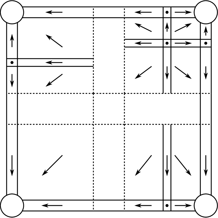
[t] at 305 9 \pinlabel [r] at 9 305 \endlabellist
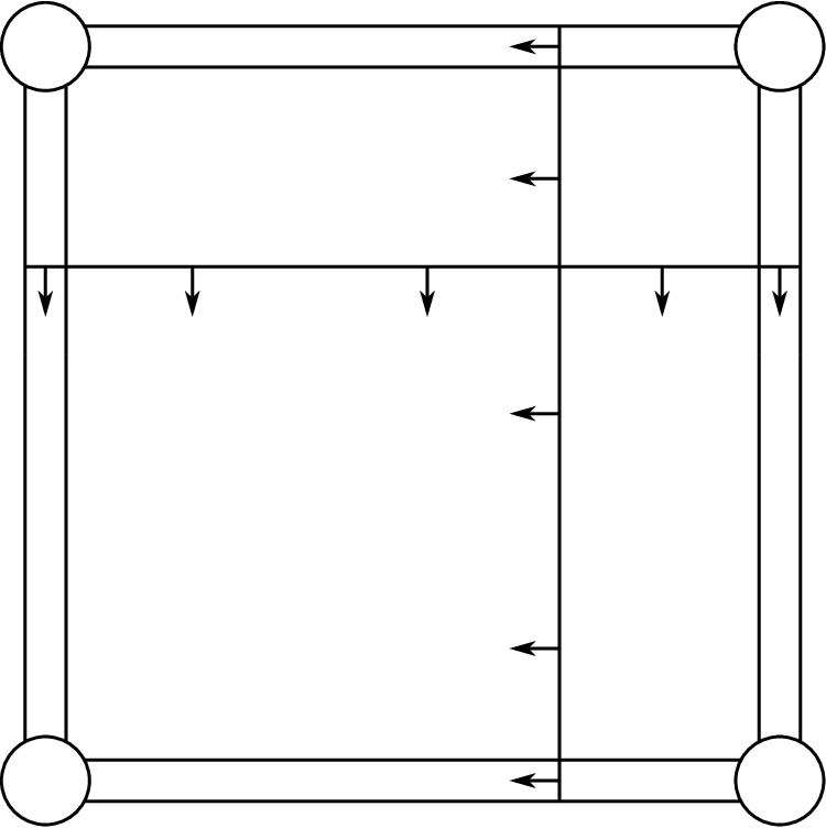
Property 12.
There are line segments and , such that the following hold.
- •
The segment begins on , ends on and is contained in the rectangle .
- •
For all , and with , is transverse to and points in to the region above .
- •
The segment satisfies analogous conditions with all locations reflected across .
See Figure 33, below, where portions of the segments and are pictured.
6.3.1. Transversality at cusps
Recall from Section 2.2 that if sheets and meet at a cusp, then a point along the -cusp edge where or is tangent to the (base projection) of the cusp locus for some above or below is called an - or -switch point. Note also that along the cusp locus and .
Property 13 (Cusp transversality).
For a square of type (1)-(11), suppose sheets form a cusp edge. Then, at any point, where (resp. ) is above (resp. below) the cusp edge the vector fields , , and are transverse to the cusp locus and point towards the region with fewer sheets.
In each Type (12) square, the above condition holds with the following exception: With sheets labeled as they appear above such that and meet at the cusp edge, there is a unique non-degenerate -switch point, , located with -coordinate above the point where the crossing locus and the cusp locus intersect and below . Between and , is transverse to the cusp locus and points towards the region with more sheets.
See Figure 30.
[bl] at 64 134 \pinlabel [r] at 50 65 \pinlabel [l] at 198 98 \pinlabel [l] at 198 34 \endlabellist

6.3.2. Stable manifolds of the
For , any Reeb chord or is a saddle point of , and has stable manifold, with respect to , consisting of the point itself and two non-constant flow lines that limit to the point as . Moreover, Proposition 5.11 shows that precisely one of these flow lines is contained entirely in . (The other flow line is contained in the other -cell that borders .) We refer to this non-constant flow line as the -line or the -line in .
[r] at 10 64 \pinlabel [l] at 358 104 \endlabellist

Lemma 6.7 (Limits of -lines).
For squares of type (1)-(12), as the -line limits to (resp. ) if (resp. if ), while (if it exists) the -line limits to (resp. ) if (resp. if ).
See Figure 31.
Proof.
Follow the flow line, , as decreases towards . Once enters it cannot leave (by Property 3). Moreover, as , must either limit to a critical point of , or terminate at a cusp edge. (Since increases as decreases, the flow line cannot terminate at a crossing.) The only critical point of in with is (resp. ), so the result follows once we show that cannot terminate at a cusp edge.
Suppose does terminate at a point of the cusp edge. Then must point to the side of the cusp locus where more sheets exist, and one of or must be a cusp sheet. [Near a cusp locus, is only defined on the side where and both exist. Therefore if runs into a cusp locus involving or it must approach this cusp locus from the side where and both exist, and since we follow in the direction where decreases it follows that points to the side of the cusp locus where and both exist.] By Property 13, the square is then of type (12) with and , so belongs to either the stable manifold of or . [These are the only Reeb chords with upper and lower sheets and respectively.] However, by Proposition 5.11, these stable manifolds enter in the upper right corner where and . Then, Property 10 shows that the stable manifolds of or must remain in the region where and , so they cannot reach the cusp locus. ∎
6.3.3. Non-existence of switches and vertices
Proposition 6.8.
Consider any 2-cell of of type (1)-(12). No GFT in has a - or -vertex.
Proof.
The image of a -vertex must be at a point on the cusp locus. Moreover, at this image there there must be sheets and that respectively lie above and below the cusp edge and have the property that points into the side of the cusp locus where the number of sheets increases by . Such a point cannot exist by Property 13.
Property 13 also states has a switch point only when is a Type (12) square. Then, there is a unique switch point with -coordinate above the intersection of the crossing and cusp loci. We show that a switch cannot occur at this point in any PFT. If this were to happen, the outgoing edge of the switch would be a -flow line, , that begins at the switch point. By Property 10, cannot cross into the region where and . There are no critical points of in the part of with outside of , and and do not meet at a cusp edge. Thus, if it did not end at an internal vertex, would only be able terminate at the cusp or crossing locus, and would not be part of a valid PFT. Now, if ends at an internal vertex it can only be a that occurs above the -crossing locus. The two outgoing branches of the will be a -flow line and a -flow line. However, the -branch cannot be completed to a valid PFT. Indeed, Property 10 applies to show the flowline stays in the complement of where there are no critical points of with , and there is no -cusp edge. Thus, if it were part of a PFT, then this edge would have to end with an internal vertex. However, and have no sheets between them in the region where , so this edge cannot end at a - or -vertex. Moreover, the edge cannot end at the -switch point, since the difference between -coordinates of sheets strictly decreases along all non-constant edges of a PFT. ∎
Proposition 6.9.
For a square of type (1)-(12), any GFT starting at one of the generators or is rigid if and only if
where and denote the number of endpoints at generators of the form and or respectively, and denotes the number of endpoints at -vertices.
6.4. Rigid GFTs with at least one output
The computation of , as stated in Theorem 6.5, is accomplished in two parts. In this section, we verify those terms in that correspond to rigid GFTs with at least one output at a Reeb chord. Then, in 6.5 we identify the remaining terms in .
For , we introduce the notation
where the sum is over those rigid GFTs, , with an input at and having at least one output vertex at a Reeb chord of the form or .
Theorem 6.10.
For a -cell of type (1)-(12), and for any , we have
| (10) |
where the matrices , and are as in Theorem 6.5, and is a matrix whose entries belong to the -sided ideal generated by exceptional generators in .
6.4.1. The First and Third Quadrant Lemmas
Recall that we have coordinates where is obtained by removing interiors of the . Now, take the full upper right corner of ,
and remove the vertical and horizontal bands
This results in four regions that we call the -quadrants and denote by where
and the numeration proceeds in a counter-clockwise manner. In addition, let and denote thickened versions of and defined by
See Figure 32.
[r] at -2 50 \pinlabel [l] at 490 126 \endlabellist

Lemma 6.11 (First Quadrant Lemma).
Let . Any PFT, , that begins with an -flow line at a point in has all endpoints at generators. Moreover, the image of is entirely contained in .
Proof.
For any , (5) implies that Moreover, Properties 7 and 10 imply that an -flow line that begins in cannot leave as -increases (since points inward along all portions of the boundary of ). Within , sheets appear in the same order that they are indexed, so any branch of the PFT tree that is below the initial -flow line can only be an -flow with . (Any -vertices, including punctures, can only increase the first subscript and decrease the second.) The result then follows, since the only Reeb chord with upper and lower sheets and contained in is . ∎
Lemma 6.12 (Third Quadrant Lemma).
Suppose and .
Then any PFT beginning with an -flow at has
- (1)
all endpoints at ’s and -vertices, or
- (2)
at least endpoint at an exceptional generator.
Proof.
We begin by establishing the following Lemma.
Lemma 6.13.
Consider a PFT, , that begins with a -flow line at a point , for some . Let be a path beginning at and consisting of several consecutive edges of , (each parametrized according to their orientation in ). The path must cross into before leaving .
Proof of Lemma 6.13.
[l] at 214 158 \pinlabel [b] at 158 214 \pinlabel [l] at 172 42 \pinlabel [b] at 42 172 \pinlabel [r] at 122 80 \pinlabel [t] at 80 122 \pinlabel [t] at 32 -2 \pinlabel [r] at -2 32 \pinlabel [t] at 128 -2 \pinlabel [r] at -2 128 \pinlabel [t] at 208 -2 \pinlabel [r] at -2 208 \pinlabel [r] at 160 160 \endlabellist

Consider the (non-convex) hexagonal subset of bounded by line segments Here, and are the segments from Property 12; is the vertical segment from to the right endpoint of ; and is the vertical segment from to the left endpoint of . The remaining segments are obtained from reflecting across . See Figure 33.
The region satisfies
Therefore, the path which begins in must leave to leave . Initially, is a -flow line with . Moreover, until we leave the only type of vertices that may appear in are -vertices. [This is because the cusp locus is disjoint from .] Within the sheets of appear in the order that they are indexed, thus after a , either outgoing edge is, for some , an -flow line. In particular, the edges that constitute consist of such flows as long as remains in . Property 12 then shows that when leaving the path cannot cross or , and Property 10 shows cannot cross our of along or . Therefore, must leave along one of the segments or , and immediately afterward its image lies in . ∎
We return now to the proof of Lemma 6.12. Consider an endpoint of a partial flow tree satisfying the stated hypothesis. Let denote the portion of the tree that travels from to this endpoint. Applying Lemma 6.13, at some point the path is in . The proof will now be completed by applying the following Lemma 6.14 to the PFT that consists of the subset of below .
∎
Lemma 6.14.
Any partial flow tree with initial point in has
- (1)
all endpoints at ’s or -vertices, or
- (2)
at least endpoint at an exceptional generator.
Proof.
Let and so that .
We prove the stronger statement that any PFT with initial point in satisfies (1) or (2).
Claim 1. If sheets with do not have a crossing arc on the (resp. ) and do not meet at a cusp above the (resp. ) edge, then (resp. ) is invariant for the -flow, i.e. is invariant in positive time.
This follows since together Properties 2, 3, 7, and 11 show that points inward along all portions of the boundary.
Claim 2. Any partial flow tree starting with a -flow line with has an endpoint at an exceptional generator.
At the first -vertex, the -flow will split into edges that are -flows and -flows. Since , we will have either or . Proceeding inductively, we can then find an endpoint that limits to a Reeb chord whose upper endpoint is on a sheet with larger label than the lower endpoint. All such Reeb chords are exceptional.
Claim 3. Consider a square that has crossings along the edge , i.e. of type (5), (6), (8) or (12), so that along sheet crosses sheets and . [Sheets are labelled as they appear at .] Then, any partial flow tree that begins with a -flow in has at least one endpoint at an exceptional Reeb chord.
From Claim 1, we see that is -invariant. [In any of the 12 squares, it is never the case that the same two sheets cross on both the edges and .] Observe that there are in fact no non-exceptional Reeb chords in (and, in the case of a Type (12) square, no cusp edge). Thus, such a partial flow tree without -vertices would necessarily contain an exceptional generator. In all cases except for Type (8), sheets and are always adjacent in , so no -vertex can occur. For a Type (8) square, the only portion of where a -vertex may occur in a -flow is in the portion of the square where sheets appear in the order . See Figure 34. One of the outgoing branches of such a -vertex would be a -flow, and Claim 2 would then imply that the tree has an endpoint at an exceptional generator.
[l] at 228 160 \pinlabel [l] at 228 80 \pinlabel [l] at 228 0 \pinlabel [r] at -4 160 \pinlabel [r] at -4 80 \pinlabel [r] at -4 0 \endlabellist

With Claims 1-3 in hand, suppose that we are given a partial flow tree in a square of type (1)-(12) that begins with an -flow at . In establishing the conclusion of the lemma, by Claim 2, we may assume . We first treat all of the special cases in which the and sheets cross or meet at a cusp edge, and then address the remaining cases inductively. Note that an crossing or cusp arc cannot have endpoints on both the and edge.
- •
Case 1: The crossing arc does have a single endpoint on edge or . This includes the squares of type (2), (4)-(8), (10), (12) where can correspond to any of the crossing arcs. Note that for any of the squares (5), (6), (12) with , Claim 3 applies. The remaining cases are as follows:
- –
Subcase 1: The square is any of (2), (4), (7), (10) with any of the pictured arcs.
First consider the case where the crossing occurs on edge . Then, from Claim 1, is -invariant. Moreover, in the subset of where , the sheets and are adjacent so that there are no possibilities for a partial flow starting at to have -vertices. Finally, observe that the only non-exceptional Reeb chord in is at . [For a general square, the only non-exceptional Reeb chords in are and , but in the present case there are no Reeb chords of the form and as they would necessarily on the other side of the crossing arc.]
If the crossing occurs on edge , a similar argument (reflected across ) applies.
- –
Subcase 2: The square is (5), (6), or (12) with . Again, is invariant, and the only non-exceptional Reeb chord in would have the form . Thus, in the case there are no -vertices the result follows. If the flow tree has -vertices, then at the first -vertex the tree splits into a -flow and a -flow in the region above the -crossing arc. Now, an application of Claim 3 shows that the flow tree must contain an exceptional generator.
- –
Subcase 3: The triple point square (8). The case is covered by Claim 3. For , the partial flow tree must have an end point at an exceptional generator. This follows since is -invariant and contains no non-exceptional Reeb chords of type The only possibility for a -vertex would produce an outgoing edge that is a -flow to which we apply Claim 2. (See Figure 34.)
Finally, consider . The -flow is -invariant with all Reeb chords in exceptional. If a -vertex occurs one out going edge will be a -flow in which must have an endpoint at an exceptional generator by Claim 3.
- –
- •
Case 2: The crossing arc has its endpoints on edges and This only occurs in (3) with . Here, Claim 1 gives that is -invariant. In this region, sheets and are adjacent and all Reeb chords are exceptional.
- •
Case 3: The cusp edge has its endpoint on or . Supposing the cusp edge lies on , Claim 1 shows that is invariant. As they are adjacently indexed, any would produce an outgoing edge that is a -flow with , and Claim 2 would then produce an exceptional generator. Since there are no Reeb chords in , if the PFT has no ’s, then the -flow necessarily reaches an -vertex.
With the special cases out of the way we handle the general case using induction on the number of -vertices in the partial flow tree. Since we can assume that the sheets do not cross, Claim 1 shows that the quadrant is -invariant. The only -Reeb chord in is , so in the case of no -vertices the result holds. For the inductive step, at the first -vertex, an -flow line splits into a -flow line and a -flow line for some . Since is invariant, the inductive hypothesis applies to both partial flow trees below the -vertex. ∎
Proof of Theorem 6.10.
The matrix formula (10) is equivalent to the term-by-term formula
| (11) |
where any of the terms which correspond to Reeb chords that do not exist or are exceptional generators are replaced with , except that is replaced with if and meet at a cusp edge in ; the is an element of the ideal generated by exceptional generators in . We show that, aside from , each of the non-zero terms in (11) corresponds to an odd number of rigid GFTs beginning at and that any other rigid GFTs with an output at some or must have endpoints at exceptional generators.
For each of the (non-zero) quadratic terms of (11) we now observe a single GFT beginning at (and rigid by Proposition 6.9) whose word agrees with the given term.
Term 1: for .
Travel along the unique -flow line beginning at that intersects . Once this point is reached a puncture occurs. That is, a -vertex appears where the two outgoing edges are an -flow line and the constant -flow line at . Since , the non-constant outgoing edge is an -flow line that limits to an output vertex at by Lemma 6.11. See Figure 35.
Term 2: for . Travel along the -flow line that hits , and then puncture. Since , Lemma 6.12 shows that the outgoing -flow line behaves as follows:
- (1)
It limits to as long as and do not cross and they both exist at .
- (2)
If and cross, then if the crossing locus separates from the flow line runs into the crossing locus (and is not part of a valid GFT). In the case that the crossing locus does not separate from , as can happen for Type (4) or (6) squares, the flow line may either run into the crossing locus or end at . For such squares, is an exceptional generator so the precise behavior is not relevant.
- (3)
If or meets a third sheet in a cusp edge, then the -flow line ceases to exist when the cusp edge is reached (and is not part of a valid GFT).
- (4)
If and meet one another at a cusp, then the flow line reaches an -vertex at the cusp edge. In this case we do have a valid rigid GFT.
Note that the results described in (2) and (3) are consistent with the entries that appear in as a result of crossings or cusps. Replacing the -entry of with a when and meet at a cusp edge is consistent with (4). See Figure 35.
[b] at 40 164 \pinlabel [t] at 56 92 \pinlabel [t] at 0 68 \pinlabel [r] at 162 48 \pinlabel [br] at 220 110 \pinlabel [l] at 286 162 \pinlabel [b] at 408 164 \pinlabel [t] at 392 92 \pinlabel [t] at 448 68 \pinlabel [br] at 644 141 \pinlabel [t] at 640 110 \pinlabel [r] at 506 10 \endlabellist

Proof of uniqueness. We have thus identified a single rigid GFT for each of the (non-zero) terms in (11) aside from . To complete the proof, we show that these are the only rigid GFTs beginning at with at least one output at some or and without any outputs at exceptional generators. We follow the outline indicated in Figure 36.
Let be a rigid GFT that begins at some , , without endpoints at exceptional generators and having at least one puncture at some or . In the latter case, we are done since is an exceptional generator.
Step 1. If has an -edge that punctures at (resp. ), then there are no further internal vertices on the non-constant branch that follows the puncture. Thus, after the puncture agrees with the GFT found in Step 1 (resp. Step 2).
The critical point is located in . Therefore, the PFT starting with the non-constant branch following the puncture begins with a -flow in , and Lemma 6.12 implies all endpoints below the puncture must be at Reeb chords or -vertices. A similar argument with Lemma 6.11 used in place of Lemma 6.12 shows that all endpoints below a puncture at must be at Reeb chords. Since Proposition 6.8 shows that any internal vertices of must be ’s, the number of outputs of the PFT that starts below the puncture will be equal to the number of ’s plus . However, Proposition 6.9 states that the total number of outputs of at Reeb chords and -vertices must be the same as the number of outputs. Thus, there can be only one or -vertex below any puncture, so after the puncture there are no -vertices and Step 1 follows.
In addition, Proposition 6.9 together with Step 1 show that:
| (12) | Any edge with its endpoint at an or -vertex must begin with a that is a puncture at a . |
[As we have seen, any puncture at a Reeb chord has its non-constant branch ending at an or an -vertex. This, gives an injection from the set of endputs of to the set of endpoints of at Reeb chords and at -vertices. Proposition 6.9 shows that this injection is actually a bijection.]
[b] at 35 229 \pinlabel [b] at 163 229 \pinlabel [b] at 339 229 \pinlabel [b] at 467 229 \pinlabel [b] at 35 68 \pinlabel [b] at 339 68 \pinlabel [t] at 320 186 \pinlabel [t] at 53 186 \pinlabel [t] at 2 153 \pinlabel [t] at 130 153 \pinlabel [t] at 194 153 \pinlabel [t] at 371 153 \pinlabel [t] at 434 153 \pinlabel [t] at 498 153 \pinlabel [t] at 2 -2 \pinlabel [t] at 130 -2 \pinlabel [t] at 194 -2 \pinlabel [t] at 371 -2 \pinlabel [t] at 434 -2 \pinlabel [t] at 498 -2 \pinlabel [t] at 66 -2 \pinlabel [t] at 306 -2 \pinlabel [b] at 162 102 \pinlabel [b] at 466 102 \pinlabelStep 2: [r] at -10 32 \pinlabelStep 1: [r] at -10 192 \endlabellist

Step 2. In (the domain of) a puncture at a cannot appear below any internal vertex, .
By Proposition 6.8 the internal vertex can only be a -vertex.
- Case 1:
Assume , and an -flow branches at into the -flow to some and a -flow.
-
Subcase : Introduce the notation
which may be approximately viewed as a square with lower left corner at and upper right corner . See Figure 37. According to Property 10, points outward along each of the edges of . Therefore, as we follow the -edge with decreasing , from its end at towards its beginning at , the edge cannot leave the square. Thus,
and we apply Lemma 6.12 to the -branch that starts at to arrive at a contradiction of (12).
\labellist\pinlabel[l] at 94 90 \pinlabel [r] at 155 159 \endlabellist

Figure 37. The square, . For any such that with respect to lexicographic order, points outward along all edges of . -
Subcase : A similar argument shows
and we again apply Lemma 6.12 to the -branch starting at to deduce a contradiction.
-
- Case 2:
Assume , and an -flow branches at into an -flow and the -flow to .
At this point, as a consequence of Steps 1 and 2, we see that must be one of the trees identified in Terms 1 and 2 above. This completes the proof.
∎
6.5. Rigid GFTs without outputs at any
For , let
where the sum is over rigid GFTs that do not have outputs at Reeb chords of the form or .
Theorem 6.15.
For a -cell of type (1)-(12), and for any , we have
| (13) |
where the matrices , and are as in Theorem 6.5, while is a matrix whose entries belong to the -sided ideal generated by exceptional generators in .
We prove Theorem 6.15 at the conclusion of this section after reducing the computation to a purely topological problem.
6.5.1. -trees
Lemma 6.16.
In where has type (1)-(12), any rigid GFT starting at a and without outputs at Reeb chords of the form or must have
- (1)
all outputs at Reeb chords of the form or with ; and
- (2)
all internal vertices are ’s.
Definition 6.17.
A -tree is a PFT or GFT that satsifies conditions (1) and (2) from Lemma 6.16 and also has
- (3)
no outputs at exceptional generators.
Define a -tree to be a -tree with all endpoints at and/or Reeb chords. Define a -tree in a similar manner.
For , define a region to be the closed subset that is
- •
bounded on the right by ;
- •
bounded below by (i) the horizontal segment from to the barrier from Property 12; (ii) the part of the barrier that lies between and ; and (iii) the horizontal segment at from to the left boundary of ; and
- •
bounded on the left and above by .
In addition, define regions to be the reflection of across the line . See Figure 38.
[br] at 328 142 \pinlabel [l] at 380 128 \pinlabel [t] at 344 92 \pinlabel [l] at 238 32 \pinlabel [r] at -2 0 \endlabellist

Lemma 6.18.
Any edge, , of a -tree (resp. a -tree) must
- (1)
be an -flow line for some and
- (2)
have the intersection of its image with contained in the region (resp. ). Moreover, the image of is entirely in unless is part of a -line for .
(The terminology -line from (2) is as in 6.3.2.)
Proof.
First, in some cases, we need to focus on certain subsets defined by
- (1)
if either and cross above or meet one another at a cusp above ;
- (2)
when exactly one of and ends at a cusp edge above ; and
- (3)
in all other cases.
Observe that that points outward along all segments of . [With as in (1), for boundary segments that are not part of , just use Properties 10, 11 and 12; as in (3) add Properties 11; as in (2) add Property 13.]
We prove the proposition by establishing the same result with each replaced with (this is a stronger statement) using induction on , the number of ’s in the PFT beginning with . By Proposition 5.11, all of the - and -lines intersect at a point in . [Note that if is as in (1) or (2) then there is no -line.] It follows that as decreases they must remain in . Thus, the case holds.
For the inductive step, consider the at the end of . Both of the PFTs that begin with the outgoing edges of the are themselves -trees. Thus, by the inductive hypothesis, this has its image in for some with . [Note that the parts of the - and -lines that lie outside of are contained in disjoint strips in and and cannot intersect one another.] Thus, the result follows once we verify that:
Claim. For any Type (1)-(12) square, , for all , we have .
That
holds in general. [The second inclusion is easily verified using the lexicographic ordering of the . See Figure 39.] Thus, when the Claim follows. Now, if is as in (2), then at least one of the pairs and includes a sheet that ends at a cusp edge above , and so at least one of or lies entirely to the right of so that
Finally, if is as in (1), then the only way that there exists with is when has two crossings, i.e. Type (2Cr), above , and . Since sheets and also cross in this case, is also as in (1), and we see that
∎
[l] at 252 152 \pinlabel [l] at 156 56 \pinlabel [l] at 204 104 \pinlabel [b] at 0 198 \endlabellist

Proposition 6.19.
Any -tree is either a -tree or a -tree.
Proof.
Use induction on the number of ’s and Lemma 6.18. At the inductive step, note that the regions and are all disjoint except when . ∎
6.5.2. Topological preliminary
Let be a (region diffeomorphic to) a closed disk in . Suppose that we are given a collection of points and a collection of closed intervals with . In addition, suppose that
- •
the points and intervals are all pairwise disjoint from one another, and
- •
each point is assigned an upper index and a lower index that are integers with .
We refer to such a triple as a disk datum.
Definition 6.20.
A generalized -manifold for the disk datum is a collection of (embedded) paths in with the following properties:
- (1)
Each path has upper and lower indices, , satisfying .
- (2)
For any , the initial point of belongs to .
- (3)
For , paths in are in bijection with (i) points , with , and (ii) triples where , , , that satisfy , and .
- (4)
A path corresponding to a point as in (3) (i) has its endpoint at and satisfies .
- (5)
A path corresponding to a triple as in (3) (ii) has its endpoint at and satisfies .
- (6)
All intersections between distinct are transverse. Moreover, the only case when intersections can occur at endpoints of a path, or when three paths meet at a common point is as specified in (5). There are no points where four or more paths intersect.
See Figure 40 for an example of a generalized -manifold.
For each path , we assign a word, , that is a formal product of points from , and a sign, , as follows.
- •
For corresponding to a point as in (3) (i), let and .
- •
For corresponding to a triple as in (3) (ii), let and . Here, is the intersection sign of at . (We assume an orientation on is fixed.)
For , we define an element in the free associative -algebra generated by by
| (14) |
where the sum is over those that begin on (We introduce here a -algebra instead of a -algebra because we hope to generalize our main DGA computations to -coefficients in a future paper. For this article, however, the reader can think of )
[tr] at 28 12 \pinlabel [tl] at 132 12 \pinlabel [bl] at 148 134 \pinlabel [b] at 80 164 \pinlabel [br] at 12 134 \pinlabel [bl] at 103 43 \pinlabel [br] at 57 43 \pinlabel [r] at 80 118

Main Example. Consider a Type (1)-(12) square, , such that has sheets above . We let be obtained from by removing the small squares that contain the . Let be the upper and left sides of the closed square . By a slight abuse of notation, for , we use and to denote the unique intersection point of the stable manifolds of these critical points with the boundary of . (Note that is only defined for those such that sits above along the upper half of .) The triple is a disk datum, where the upper and lower indices of the points are given by their subscripts. See Figure 41.
[tl] at 254 64 \pinlabel [tl] at 318 128 \pinlabel [tl] at 382 192 \pinlabel [br] at 236 86 \pinlabel [br] at 306 156 \pinlabel [r] at 360 208 \pinlabel [b] at 376 254 \pinlabel [b] at 312 254 \pinlabel [b] at 248 254 \pinlabel [r] at -2 72 \pinlabel [r] at -2 136 \endlabellist

We will define a generalized -manifold for the disk datum . Suppose that is the top branch of a GFT that is a -tree beginning at some , and let . In addition, define upper and lower indices , so that is a trajectory for , i.e. and are the sheets of that correspond to in the GFT that it belongs to.
Proposition 6.21.
Let denote the collection of such paths with and as above. Then, is a generalized -manifold for the disk datum . Moreover,
where the sum on the right is over -trees that start at , and denotes with coefficients reduced mod .
An analogous result holds for -trees.
(Recall that the word, , of a GFT, , was defined in Section 2.2.1.)
Proof.
The condition (1) in Definition 6.20 is clear. Condition (6) is one of the transversality conditions that is implied by being -regular.
The top most branch of a -tree, , must start at some . Since , and (by Lemma 6.18), we see that, as increases from , must enter along a unique point in . [Uniqueness follows since points outward along the entire boundary of .] Thus, (2) holds.
Now, as , must either (a) limit to a critical point or or (b) end at a that occurs at the intersection of two edges of , and , with . Clearly, those satisfying (a) are in bijection with as in (3) (i) and satisfy (4). When satisfies (b), note that, when extended to allow , the branches and are themselves the top branches of unique -trees. Thus, the satisfying (b) are in bijection with intersection points as in (3) (ii) and satisfy (5).
The equality is clear since the word associated to a path that is a top branch of the -tree is precisely the word . [This is verified by an obvious induction.]
∎
The following key proposition will allow us to compute without requiring detailed knowledge of the locations of -lines.
Proposition 6.22.
For any disk datum , the sums are independent of the choice of generalized -manifold, , associated to .
Proof.
We prove the following statement by induction on with decreasing from to :
Inductive Statement: Let and be two generalized -manifolds for such that
| for all . |
Then, for all ,
where and are elements of as defined in (14).
The case is tautological. For the inductive step, suppose that the statement is known for larger values of , and suppose for . Notice that paths in and are in bijection, and have the same endpoints and indices. [The number of paths in as well as their endpoints and indices are determined by the and intersections of paths in .] Thus, without loss of generality, we may assume that and are identical except for a single pair of paths and with the same endpoint and equal indices.
Since is a topological disk, and and are smoothly embedded arcs with the same endpoints, they are isotopic via an isotopy of arcs , , with and that preserves endpoints.
Set
By standard transversality results, after possibly modifying the isotopy , we may assume that there exist such that, the are transverse to all paths in , and for either:
- O.
The paths in are obtained from the corresponding paths in by applying an orientation preserving diffeomorphism .
Or, when , remains fixed except in a small disk where one of the following four moves occurs:
- I.
The disk intersects a single path in a properly embedded arc. For some , has a tangential intersection with that results in the creation or cancellation of two transverse intersections.
- II.
Suppose has its endpoint at a transverse crossing point, , of paths . The disk contains , and for some , becomes tangent to either or at resulting in the addition or removal of a single transverse intersection between and or .
- III.
The disk contains a crossing, , of two paths . Note that if and have a common upper and lower index, then may be the endpoint of a third path . Both and have a single intersection point with in , and these intersection points lie on opposite sides of . The same holds for intersections of and with . If exists, then precisely one of and intersects in , and this intersection is unique.
- IV.
The disk contains on its boundary part of the interval where has its initial point. For the endpoint of passes the location of the endpoint of another path whose endpoint also lies on . This creates or removes a crossing between and .
See Figure 42 for a depiction of Moves I-IV.
I. [r] at -6 300 \pinlabelII. [r] at 612 300 \pinlabelIII. [r] at -6 80 \pinlabelIV. [r] at 612 80

Making use of the inductive hypothesis, it suffices to establish the following:
Claim. For any , there exist some generalized -manifolds, and for such that ;
We prove the claim when and are related by Moves O and I-III in a case-by-case manner.
Move O. Extend to obtain a generalized -manifold as follows. Take for , and . We then define with inductively. With all having already defined, the required number of paths in as well as their endpoints and indices are specified by and according to Definition 6.20. We then define by choosing some collection of paths with the desired endpoints that are transverse to all paths in and to one another. [Note that in order for Definition 6.20 to be met, any new intersection points with and , for some , and such that either or will have to be the endpoint of some path in with . Since , this will be arranged at a later step of the induction, and in particular will not require any modification of the already defined subsets .]
The construction of is thus completed after finitely many such steps. We then arrive at by applying the diffeomorphism to each of the paths in .
In considering Moves I-IV, we assume without loss of generality that (resp. ) corresponds to the diagram on the left (resp. right) as depicted in Figure 42. To simplify notation, we let and denote and as they appear on the left and right side of Moves I-IV.
Move I. As in Move O., extend to a generalized -manifold , but at the inductive step impose the additional requirement that all new paths are disjoint from . Unless or , is obtained from by simply replacing with .
Consider now the case where or . Form from by replacing with . We need to add two additional paths and to that end at the intersection points and of and that appear on the right side of Move II. Do so by choosing a single path from the right side of to (where and are as specified by the indices of and ). Then define and to travel from and to the initial point of , and then follow parallel to until they reach . We take and to be close enough to one another so that their intersections with paths in are are in bijection with one another with the same signs, and are located in small neighborhoods of the intersection points of . Set . See Figure 43.
Now, the new paths and may have corresponding intersection points and with some , such that for , or . For each such pair of intersections, we connect and to the appropriate using a pair of sufficiently close paths, and then denote the union of with all such pairs of paths as . We proceed inductively, and note that at each step the difference increases for all new paths. Thus, this process terminates after less than steps, and we take to be the resulting generalized -manifold.
To verify that , note that . Now, , and paths in that begin at come in pairs (as constructed in the previous paragraph), and , such that and (since the two intersections of with have opposite signs). Such pairs cancel out in the sum from (14) that defines .
[r] at 86 142 \pinlabel [r] at 46 84 \pinlabel [b] at 144 88 \pinlabel [t] at 144 72 \endlabellist

Move II. Since the indices of the , , must be of the form and for some , and , we have and . Thus, we can take to be any extension of with all new paths disjoint from , and set .
Move III. Let denote the two paths of that cross in . In our figures we picture with negative slope and with positive slope. Label the intersection points in as , , and for . See Figure 44.
Introduce the following notation for indices:
Recall that there may be an additional path that intersects and has its endpoint at . If it exists, in , intersects precisely one of and , and this intersection is in a single point. Without loss of generality we assume that, within , is disjoint from and intersects precisely once. [If this is not the case, then interchange the left and right side of Move III and rotate the diagrams by .]
To begin, choose an extension of to a generalized -manifold, , so that any paths starting at , , and (should they exist) are respectively disjoint from , , and . Denote these paths by , , , and note that it may be the case that . See Figure 44.
[br] at 22 140 \pinlabel [bl] at 156 140 \pinlabel [r] at -2 82 \pinlabel [b] at 57 114 \pinlabel [b] at 120 114 \pinlabel [t] at 88 74 \pinlabel [t] at 384 44 \pinlabel [t] at 322 44 \pinlabel [b] at 352 88 \pinlabel [l] at 444 80 \pinlabel [br] at 284 140 \pinlabel [bl] at 420 140

[tr] at 6 50 \pinlabel [b] at 104 198 \pinlabel [tl] at 202 60 \pinlabel [tr] at 410 50 \pinlabel [b] at 508 198 \pinlabel [tl] at 606 60 \pinlabel [b] at 452 92 \pinlabel [b] at 546 142 \pinlabel [b] at 572 48 \endlabellist

To keep track of indices, it is convenient to assign a coefficient to each path , , that is the strictly upper triangular matrix whose -entry is , and with other entries equal to . We then make the observation that if two paths intersect at a point then Definition 6.20 specifies that the coefficient of the path in that ends at is
where if , then no such path exists in . Thus, we interpret a coefficient of to indicate that the path is not part of .
Above, is the commutator of matrices in . Up to a sign, has the form
Note that since the subscripts satisfy and , only one of the terms on the right can be non-zero. This implies the following:
Observation 1. Any iterated commutator of matrices of the form with again retains this form or is .
Note also that because a product of the form must be when and is upper triangular, we must have:
Observation 2. If the same appears more than once in such an iterated commutator, then the result is .
Abusing notation by writing for its coefficient , the coefficients of and are respectively
To construct , start with as follows. Take , but replace the paths , (if they exist) with new paths and that, outside of , agree respectively with and . [Since the point remains unchanged, we can retain the path , which is the only one of the three that may belong to .] We can arrange that , , , respectively have unique intersection points in with , , and . Denote these intersection points as
Now, it may be the case that additional paths starting at , and/or must be added to to form a generalized -manifold. Whether such paths are necessary, and what their indices should be are determined by the coefficients associated to these intersection points. They are
[Note that at the level of coefficients, , , and .] Moreover, the initial signs are all equal
[To verify this, note that and are all oriented toward their endpoints which appear in . Moreover, reversing the orientation of any one of changes all three quantities by a sign. Therefore, it is enough to check the equality for a single choice of orientation of . If we orient these three curves to the right as pictured, the three products become
Therefore, by the Jacobi identity, the sum of these three coefficients is
Since each of them is either or a single matrix of the form with (by Observation 1), we have two possibilities:
- (1)
All three coefficients are . This means that no additional paths are necessary, so is a generalized -manifold with the desired properties.
- (2)
One coefficient is and the other two are negatives of one another. This means that we need to add two paths starting at two of the points and and with the same indices but opposite signs. We choose these paths so that outside of they are small shift of a single path from the to the appropriate . Note that the coefficients of any intersection points in between these two new paths and existing paths must be because of the Observation 2. Then, proceeding as in Move I, we construct inductively so that all paths not corresponding to paths in cancel in pairs when computing .
Move IV. Since , Move IV may be treated as in Move II.
∎
Proof of Theorem 6.15.
From Propositions 6.19, 6.21, and 6.22 we have
where (resp. ) is any generalized -manifold associated to the disk datum (resp. ).
Thus, Theorem 6.15 follows from:
Claim. There exists generalized -manifolds and for the above disk data such that
(Here, any of the or that do not exist are replaced with .)
We construct as the construction of is identical after reflecting across .
- (1)
Connect each to with a vertical (i.e. slope ) line segment, .
- (2)
Connect each to by a piecewise linear segment (smoothed at the corner), , consisting of (i) the line segment from to , followed by (ii) the horizontal segment (i.e. slope ) from to .
- (3)
For each such that exists, the paths and intersect in a unique point. (This follows from the location of the intervals .) Connect this intersection point to via a straight line segment, .
See Figure 45.
[l] at 280 112 \pinlabel [r] at -2 88 \pinlabel [b] at 200 162 \pinlabel [l] at 238 71 \pinlabel [l] at 206 40 \pinlabel [b] at 90 106 \pinlabel [r] at 198 142 \pinlabel [l] at 222 98 \endlabellist

It is clear from definitions that has the desired form, so to complete the proof we only need to verify that is in fact a generalized -manifold. To this end, it suffices to check that the only intersections between paths for which
| (15) |
are as in (3).
Clearly, all the are disjoint from one another. When , the are horizontal lines, so because of the relative positioning of the (lexicographically ordered along the diagonal, ) and are disjoint.
To see that is disjoint from any path with lower index , note that any path of the form or is, at least when , entirely above and to the left of . However, is entirely to the right of and below . These regions are disjoint (since preceds both and lexicographically). A similar argument shows that is disjoint from paths with upper index .
Finally, we show that for any , (provided both of these paths exist). As in (2) (i), the first half of the are line segments that, for all , begin and end at on a common pair of vertical lines. [Recall that, by Property (2) of 3 the left side of is a vertical line when .] Two such segments intersect if and only if the ordering of their -coordinates is opposite along the verical lines where the left and right endpoints sit. The left endpoint of satisfies , while the right endpoint is at . Now, where is the position of the sheet above . Thus, in order for and to cross we would need to have with respect to lexicographic order. Since this would mean that which can only happen if sheets and cross above . However, in this case doesn’t exist.
∎
7. Computation of LCH, Part 3: -cells with swallowtail singularities
In this section, we compute in Theorem 7.4 the sub-DGAs when is a square of type (13) or (14). A key feature of the Type (13) and (14) squares is that some rigid GFTs contain switch vertices. This results in a differential that departs substantially from the common formula from Theorem 6.5 that applies to squares of type (1)-(12).
7.0.1. Upward and downward swallowtails
Recall from Section 3.2 that the Type (13) square contains a single upward swallowtail point while the Type (14) contains a single downward swallowtail point. The projections of the crossing and cusp locus in Type (13) and (14) squares are identical.
To simplify exposition, we consider only the case of the Type (13) square in detail while an analogous construction and computation holds for a Type (14) square. (See Remark 7.3 for more about translating the discussion of the Type (13) square to the case of a Type (14) square.)
7.0.2. Labeling of sheets and Reeb chords above the Type (13) and (14) squares
Let be a -cell of type (13). Near we label the sheets of above as with descending -coordinate, so that denote the three sheets that all meet at the swallowtail point. The sheets and that cross one another near the swallow tail point both correspond to the same sheet to the left of the cusp locus, so we cannot extend this labelling to the entire square. Instead, we use the following:
Convention 7.1.
- (1)
For , we let denote the entire sheet that sits in position at . Note that only exists to the right of the cusp locus.
- (2)
We use and to denote only the closed subset of the sheets with position and at that lies on or to the right of the cusp locus. More precisely, the base projections of and lie on or to the right of the cusp locus.
- (3)
We use to denote the sheet with base projection on or to the left of the cusp locus that extends to agree with (resp. ) when is above (resp. below) the swallowtail point; denote the defining function of by .
Thus, to the left of the cusp locus the sheets appear with decreasing -coordinate in the order .
The Reeb chords above the neighborhoods of the boundary edges and corners of are specified by Properties 2 and 3. Reeb chords above , and their locations are as in Properties 8 and 9:
- •
For all , there is a Reeb chord with
- •
Sheets and cross, so there is a Reeb chord with
As long as neither endpoint of a Reeb chord lies on we follow our earlier Convention 5.7 so that , , , , , and denote Reeb chords above the various vertices, edges, and interior of the square with upper endpoint on and lower endpoint on . There are two Reeb chords and that are decorated with tildes. They respectively lie in the lower half of the right edge and in the lower right portion of .
Convention 7.2.
If a Reeb chord has an endpoint on the sheet , then we use for the corresponding subscript when , i.e. for the the and Reeb chords, and when , i.e. for the Reeb chords.
Remark 7.3.
A similar enumeration of sheets and Reeb chords applies to the Type (14) square. There the roles of the swallowtail sheets are reversed, so that exposition of the computation of GFTs for the Type (14) square would require translating considerations applied to the sheets , , , and from the Type (13) square to considerations for sheets of the form , and . In particular, for Reeb chords in a Type (14) square with endpoints on , we use the subscript when , and when .
7.0.3. Statement of the differential
We form matrices containing Reeb chords in where has type (13). Let , , for , and denote strictly upper triangular matrices with -entries, for , given by the corresponding Reeb chord provided that it exists. For example, take for the -entry of when . In view of Convention 7.2, there are no Reeb chords with or as a subscript. We set the -entry of to be , while all remaining entries in rows and columns and are set to . Convention 7.2 also shows that there are no Reeb chords with subscript or , and we set all entries of the and rows and columns of to be . We also place a in the -entry of . The Reeb chords do not appear in any of these matrices.
A similar procedure is applied to form matrices from the Reeb chords of a Type (14) square. In this case, has entry , while all remaining entries in the and rows and columns are ; has entries in the and rows and columns.
Recall that denotes the matrix with -entry and all other entries .
Theorem 7.4.
For a -cell of type (13), in we have
where denotes a strictly upper triangular matrix with entries in the ideal generated by . In particular, the Reeb chord does not appear in the differential of any of the .
For a -cell of Type (14), in we have
where denotes a strictly upper triangular matrix with entries in the ideal generated by . In particular, the Reeb chord does not appear in the differential of any of the .
7.1. Properties of gradients
In the following we continue to use the terminology -flow line to denote a flow line for , while -flow line or -flow line refers to a flow line of or respectively. Notice that a single edge of a GFT may change, for instance, from being an -flow line to an -flow line if its image crosses the upper half of the cusp locus.
Many of the properties of squares of type (1)-(12) stated in Section 6 continue to hold for the Type (13) square. Specifically, as previously discussed, Properties 8 and 9 hold. In addition, Property 12 continues to hold as stated. The statements from Property 10 also hold and apply as well to difference functions and provided and are used when providing the restrictions on that appear in the statements of these properties. (This is consistent with the Convention 7.2.)
Proof.
Property 11 requires the following modification, and strengthening. Recall the notation .
Property 14 (Monotonicity in half spaces, Type (13) square).
The defining functions in a Type (13) square satisfy:
- •
Suppose that , and . Then, (where defined)
Moreover, for and , we also have (where defined)
and , when . - •
Suppose that , and . Then, for we have
(16) (17)
Remark 7.6.
Since sheets and cross above , we have where transposes and . Compare with Remark 6.1.
On the other hand, Property 13 requires a serious modification for Type (13) squares. This leads to many new rigid gradient flow trees.
Property 15 (Existence and uniqueness of switch points).
Let denote the closed disk centered at with radius , and let denote (the base projection of) the cusp locus within a Type (13) square. The projection of to the -coordinate is injective. The swallowtail point, , is located within along the horizontal line at a point with . At two branches of meet at a semi-cubical cusp, where the -coordinate is minimized along . For sheets and meet along , while for sheets and meet along . For , the -cusp locus and -cusp locus each project injectively to the -axis. Outside of , agrees with the vertical line .
The defining functions satisfy the following.
- (1)
For any , there is a unique -switch point along . This switch point has .
- (2)
For any , there is a unique -switch point in .
- (3)
For any , there are no -switch points in .
- (4)
There is a unique -switch point in .
Moreover, all of these switch points are non-degenerate and are located in with .
Definition 7.7.
We refer to the portion of the cusp locus with (resp. ) where sheets and (resp. and ) meet as the -cusp locus (resp. the -cusp locus).
Corollary 7.8.
- (1)
For , or , with , , is transverse to the -cusp locus at all points besides the -switch point, . Moreover, between and (the swallowtail point), points in the direction where the number of sheets increases, while at all other points points in the direction where the number of sheets decreases.
- (2)
For , or , with , , is transverse to the -cusp locus everywhere and points in the direction where the number of sheets increases. The same statement applies for except between the -switchpoint, , and the swallowtail point where points in the direction where the number of sheets increases.
See Figure 46.
Proof.
As we precede along the - or -cusp locus, the direction of transversality of to changes exactly when either becomes tangent to the cusp locus; for as in the statement of the Corollary, such points of tangency are exactly at the -switch points. [The direction of transversality must change at a switch point because all switch points are non-degenerate.] Moreover, when is near , the direction of transversality for all positive difference functions is from right to left, by Property 7. The result follows. ∎
[l] at 108 176 \pinlabel [l] at 426 176 \pinlabel [l] at 426 96 \pinlabel [r] at 60 136 \endlabellist

7.1.1. Additional monotonicity properties for squares containing swallowtails
The following Properties 16-19 provide more detailed constraints on the direction of gradient vector fields. They are used at various places during the course of the proof of Theorem 7.4.
Property 16 (The Swallowtail Barrier).
For the Type (13) square, there is a polygonal path that satisfies the following.
- (1)
The subset is a single line segment that starts on ; ends on ; and is entirely contained in .
- (2)
For all and for all with ,
points transversally into the region to the right of . - (3)
The subset has monotonic -coordinate with its right endpoint at the lower endpoint of and its left endpoint on the left boundary of . Moreover, .
- (4)
For all , and such that ,
points transversally into the region below . (We include the case of and .)
See Figure 47.
[l] at 188 138 \pinlabel [l] at 102 50 \endlabellist

Property 17 (Barrier at ).
For any , we have , , and at all points along .
Property 18 (Downward gradients when ).
For and , we have and for all where is any of or . Moreover, at points with that belong to the crossing locus, points into the region where .
Property 19 (Switch point barriers).
There exists a line segment contained entirely in with upper endpoint at the -switch point and lower endpoint on the cusp locus such that
- •
points from right to left at all points of above or on the crossing locus; and
- •
points from right to left along all of except for the endpoint on the cusp edge.
Similarly, there is a line segment contained in with endpoints at the -switch point and on the cusp edge such that
- •
points from right to left at all points of below or on the crossing locus; and
- •
points from right to left along all of except for the endpoint on the cusp edge.
See Figure 48.
7.1.2. The , , and switch flow lines and GFTs
Flow lines that end at switch points play a role in the Type (13) square that is similar to the stable manifolds of Reeb chords. In this subsection, we examine the flow lines ending at the -, -, and -switch points.
For each -switch point identified in Property 15, we call the (unique) -flow line that ends at the switch point the -switch flow line.
Lemma 7.9.
- (1)
The -switch flow line (resp. -switch flow line) limits to (resp. ) as .
- (2)
The -flow line (resp. -flow line) starting at the -switch point (resp. the -switch point) ends at an -vertex at a point on the -cusp locus (resp. -cusp locus).
Proof.
For (1), recall that any flow line must either limit to a Reeb chord or terminate at the cusp edge as . (See the discussion around Proposition 5.11.) If the -switch flow line were to terminate at the cusp edge as decreases, it could only do so at a point of the -cusp edge where points in the direction where the number of sheets increases. From Corollary 7.8, such a point must be located between the -switch point, , and the swallow tail point, . However, Property 19 prevents the -switch flow line from passing to the left of as decreases, and the portion of the cusp locus between and lies entirely to the left of . Thus, as , the -switch flow line limits to a -Reeb chord in ; the only such Reeb chord is .
A similar argument (using the statement about and the segment in Property 19) applies to show the -switch flow line begins at .
For (2), consider only the -flow line starting at the -switch point as a similar proof will establish the statement about the -flow line. Along the segment, , that starts at the -switch point, points to the left (by Property 19). Therefore, as increases, the flow must exit the triangle-like region formed by and the cusp edge somewhere along the cusp edge. Along the lower half of the cusp locus, to the left of the -switch point, points across the cusp edge from the side with fewer sheets to the side with more sheets. [This follows from Corollary 7.8 since and agree along the -cusp edge.] Thus, as increases the flow line can only reach the upper half of the cusp edge (which is part of the -cusp locus) where it ends at an -vertex. See Figure 48 (left). ∎
[l] at 70 96 \endlabellist
 \labellist\pinlabel [r] at 136 144
\pinlabel [r] at 362 14
\endlabellist
\labellist\pinlabel [r] at 136 144
\pinlabel [r] at 362 14
\endlabellist
The flow lines identified in (1) and (2) of Lemma 7.9 fit together in pairs to produce gradient flow trees starting at and respectively. Both of these GFTs contain a single switch as an internal vertex and have a single output at an -vertex. See Figure 48. We refer to these gradient flow trees as the - and -switch GFTs.
We will make use of the following constraint on the image of the -switch flow line. Let denote the region bounded
- (1)
on the left by and the -cusp locus;
- (2)
below by a path constructed from left to right from (i) the crossing locus from to the Swallowtail Barrier (from Property 16); (ii) the part of below ; and (iii) the part of the line segment between and ;
- (3)
on the right by ;
- (4)
and above by .
See Figure 49.
[l] at 60 104 \pinlabel [l] at 244 128 \pinlabel [r] at 322 214 \endlabellist
 \labellist\pinlabel [l] at 28 24
\pinlabel [r] at 422 318
\endlabellist
\labellist\pinlabel [l] at 28 24
\pinlabel [r] at 422 318
\endlabellist
Lemma 7.10.
The -switch flow line is entirely contained in .
Proof.
Note that points outward along all segments of the boundary of . [Working clockwise from , use Property 19, Corollary 7.8, 3, Property 10 (twice), Property 16, and that goes from being positive to being negative when we pass the crossing locus.] Since the -switch flow line begins at the upper endpoint of it will remain within as decreases. ∎
Next, we study the -switch flow line. Define a closed region to be bounded by the curve that, beginning at the -switch point and proceeding clock-wise, consists of
- (1)
the upper part of the -cusp locus;
- (2)
part of the upper boundary of ;
- (3)
the vertical line ;
- (4)
the horizontal line segment ;
- (5)
the part of the Swallowtail Barrier, , with and ;
- (6)
the vertical segment from to the -coordinate of the -switch point; and
- (7)
the horizontal segment from the -switch point to .
See Figure 49.
Lemma 7.11.
For ,
- (1)
the -flow line ending at the -switch point (i.e. the -switch flow line) is entirely contained in and limits to as ;
- (2)
the -flow line beginning at the -switch point limits to .
Proof.
Along each of the boundary segments (1)-(7) of we have that points outward. [Verify with Corollary 7.8, Property 3, Property 10 (used twice), then Properties 16, 17, and 18.] Thus, as decreases the -switch flow line remains in and can therefore only limit to .
To verify the claim concerning the -flow line, , that begins at the -switch point, we consider a region bounded by:
- (1)
the horizontal segment from the -switch point to ;
- (2)
the vertical segment from the -coordinate of the -switch point to the lower boundary of ;
- (3)
the portion of running clock-wise from the bottom side at to the left side at ;
- (4)
the horizontal segment from the left side of at to the swallowtail point ; and
- (5)
the portion of the -cusp locus between and the -switch point.
Note that and point inward along those parts of where they are defined. [Verify along (1)-(5) using Properties 18, 17, 3, 18 (again), and Corollary 7.8.] Thus, even though may change from being an -flow line to an flow line if it crosses the -cusp locus, as increases must be entirely contained in . The only Reeb chord in with upper endpoint on and lower endpoint on or is (which in fact has its lower endpoint on ). Thus, must limit to as . ∎
We refer to the gradient flow tree obtained by appending the flow lines from (1) and (2) together at a switch vertex as the -switch GFT.
7.1.3. The and partial flow trees
Partial flow trees beginning with certain - or -flow lines serve as a base case for inductive arguments used later in the section. In this subsection we establish some preliminary results about such PFTs.
Lemma 7.12.
The only non-constant PFTs starting with a -flow at a point in (to the right of the cusp edge and below the crossing locus) are
- (1)
PFTs consisting of a single edge with output vertex limiting to or . These flow trees are subsets of unique flow lines that exist from to or , and are respectively contained in the vertical strip
or the horizontal strip
- (2)
PFTs consisting of a single edge with output at . These PFTs are contained entirely in
- (3)
PFTs that form some subset of -switch GFT.
Proof.
First, we show that any PFT, , without internal vertices and beginning with a flow in must be as in (1) or (2). Since does not have internal vertices it must simply be a portion of a flow line that limits to a Reeb chord as . [Ending at an -vertex is impossible since there is no -cusp edge.] The only Reeb chords are and , so must begin on a point belonging to the stable manifolds of one of these Reeb chords. The stable manifolds of and must be contained in the strips and respectively, by Properties 10 and 7 (and therefore both limit to respectively as claimed). On the other hand, a point in the intersection of the stable manifold of with must be in the region bounded by the stable and unstable manifolds of and , since flow lines cannot cross.
It remains to show that the only PFTs starting with a -flow in and having internal vertices are as in (3). Consider the first internal vertex of such a PFT, . Since sheets and are adjacent in the entire region where is above , it follows that this vertex cannot be a or -vertex. Therefore, the vertex can only be a switch at the unique -switch point, so it follows that the initial edge of the PFT is indeed a subset of the -switch flow line. The edge of that begins after the switch vertex is the -flow line that begins at the -switch point. We need to show that an internal vertex cannot occur along this edge.
Suppose instead that has a second internal vertex occurs after the switch point. The only possibility is a vertex where the -flow splits into a flow and a -flow. Furthermore, the image of this vertex must be located below the -crossing locus (otherwise there are no intermediate sheets between and ), and to the left of (since by Property 19 points to the left side of ). However, the outgoing branch of the that is a -flow line cannot be completed to a PFT since we have already seen that the only PFTs starting with a -flows must have their initial point either with or somewhere along the -switch flow line. Moreover, by Property 19 the -switch flow line is contained entirely to the right of except at its endpoint. ∎
Recall the notations and .
Lemma 7.13.
The only PFTs starting with a -flow in are subsets of the -switch GFT.
Proof.
Any -flow line that starts in must remain in since Property 10 shows that points inward along the boundary segments and . There are no Reeb chords in . Thus any such PFT must have an internal vertex. Since and are always adjacent the first vertex can only be a switch at the unique -switch point. After the switch, an argument similar to that used in Lemma 7.12 shows that the outgoing -flow line cannot end at an internal vertex. ∎
7.1.4. The invariant region
Let denote the subset of obtained by removing those points that lie strictly above and to the left of the Swallowtail Barrier . Note that the boundary of consists of:
- (1)
the vertical segment ;
- (2)
the segment of with endpoints on and ;
- (3)
the portion of below ;
- (4)
the portion of that sits below and to the left of .
See Figure 50.

Lemma 7.14.
Suppose , and . Any -flow line that begins in remains in as increases (as long as it is defined). This statement includes - and -flow lines.
7.2. Enumeration of flow trees with at least one output
For a Type (13) square, , we again write
| (18) |
with the sum over rigid GFTs that begin at and contain at least one puncture at a Reeb chord of the form or .
Recall that we have labeled the Reeb chords in with the index used for chords that begin or end on .
Theorem 7.15.
We have
| (19) |
where denotes the -entry of the matrix from Theorem 7.4 and belongs to the two-sided ideal generated by and . That is,
- •
for , ;
- •
;
- •
;
- •
for , ;
- •
all remaining are zero.
The proof of Theorem 7.15 consists of two parts. In Section 7.2.2, we identify an odd number of rigid GFTs corresponding to each of the terms in the sum. Then, in Section 7.2.3, after some preliminary results, we show that any rigid GFT with a puncture at a must be one of the GFTs from our list.
7.2.1. Degree of a partial flow tree
Rigid GFTs can be identified by the following criterion.
Lemma 7.16.
Let be a Type (13) square. A GFT in that begins at some or is rigid if and only if
where (resp. ) denotes the number of endpoints at Reeb chords of the form (resp. or ; denotes the number of endpoints at -vertices; denotes the number of -vertices; and denotes the number of switch vertices.
(Recall from Theorem 2.7, that since is -regular all vertices of are either inputs, outputs, -, -, -, or -vertices.)
Proof.
This is just Proposition 2.9 since all , , and Reeb chords are respectively local minima, saddles, and local maxima. ∎
We make the following definition to help identify PFTs that may appear as part of some rigid GFT.
Definition 7.17.
7.2.2. List of rigid GFTs with punctures at ’s.
For each term in the formula for given in Theorem 7.15 we identify an odd number of corresponding rigid GFTs.
Term 1: for . The GFT begins by following the unique -flow line that limits to as and passes the location of . When the flowline reaches a puncture (-vertex) occurs. The non-constant branch after the puncture is the -flow line beginning at . In view of the lexicographic ordering of the along the diagonal , (this follows from Properties 8 and 6), we have , i.e. is to the right and above . Therefore, by Lemma 6.11 (see also Lemma 7.5), this flowline limits to as . See Figure 51.
[b] at 40 164 \pinlabel [tl] at 58 94 \pinlabel [tr] at -2 70 \pinlabel [br] at 164 52 \pinlabel [br] at 221 107 \pinlabel [bl] at 283 163 \endlabellist

Term 2: for with . Begin by following the unique -flow line from to . When the flow line reaches a puncture occurs. After the puncture the non-constant branch is the -flow line starting at . As stated in Lemma 7.5, the Lemma 6.13 is applicable in this situation, and it shows that this flow line will pass into where is the region from Lemma 7.14. Once this occurs, Lemma 7.14 shows that the limit of this flow line can only be the Reeb chord as this is the only -Reeb chord in . [Note that because of the restriction , neither the or sheet has a cusp locus in . If one of or is , then the Convention 7.2 is relevant since the sheet becomes when the flow line crosses the -cusp locus.] See Figure 52.
[b] at 16 162 \pinlabel [tr] at -2 94 \pinlabel [tl] at 57 71 \pinlabel [br] at 260 142 \pinlabel [br] at 245 126 \pinlabel [r] at 118 0 \endlabellist

Term 3: for . Begin with the unique -flow line from to , and then puncture at . By Lemma 6.13 and Lemma 7.14, the -flow line that begins at must then enter and remain in where it can only end at an -vertex along the lower half of the cusp edge where sheets and meet; this produces a flow tree as in Figure 53.
[b] at 16 162 \pinlabel [tr] at -2 94 \pinlabel [tl] at 57 71 \pinlabel [br] at 260 142 \pinlabel [br] at 245 126 \pinlabel [r] at 179 19 \endlabellist

Term 4: for .
Again by Lemmas 6.13 and Lemma 7.14, the -flow line ,that starts at enters and remains in where it can only terminate at the -cusp locus.
Consider the closed subset , consisting of the part of that sits to the right of the cusp locus with the upper right corner removed just below and to left of , and the lower right corner removed just above and to left of . More precisely, remove
and
Now, is homeomorphic to , and the intersection of and the -switch flow line, , with are closed intervals with their endpoints on . [That the intersections of these flow lines with consist of single arcs follows from Property 10.] Moreover, the endpoints of , , and the endpoints of , , appear cyclically in the order . As and intersect transversally (by the -regularity of ), standard differential topology shows that they intersect in an odd number of points, .
To produce an odd number of GFTs: Begin with the -flow line from to , and puncture at . Follow until it reaches one of the . At , a -vertex occurs so that the outgoing edges are a -flow line, , and a -flow line, . Since , must remain in and will thus terminate at an -vertex along the -cusp edge; ends at a switch vertex at the -switch point that is followed by a -flow line that terminates at the cusp edge.
See Figure 54.
\labellist\pinlabel [b] at 16 162
\pinlabel [tr] at -2 94
\pinlabel [l] at 24 112
\pinlabel [tl] at 58 30
\pinlabel [tr] at 16 56
\pinlabel [br] at 260 142
\pinlabel [br] at 245 126
\pinlabel [r] at 186 100
\pinlabel [r] at 186 24
\pinlabel [t] at 252 24
\endlabellist
Term 5: for .
We identify an odd number of GFTs, each of which has initial branch consisting of the -flow line from to The -flow line beginning at will enter (by Lemma 6.13). Next, by Lemma 7.14 this flow line will proceed to terminate at a point on the -cusp locus. Along its way it will intersect the switch line transversally in an odd number of points, . [The reasoning is as in Term 4.] To construct GFTs , after the puncture we follow the -flow line starting at to one of the where a occurs. The branch that is a flow will then proceed to (again by Lemma 7.14), so a GFT of the form pictured in Figure 55 results.
[b] at 16 162
\pinlabel [tr] at -2 94
\pinlabel [l] at 24 112
\pinlabel [t] at 72 53
\pinlabel [t] at 16 28
\pinlabel [br] at 260 142
\pinlabel [br] at 245 126
\pinlabel [r] at 186 100
\pinlabel [tr] at 120 0
\pinlabel [t] at 252 24
\endlabellist
Note that by Lemma 7.16, the GFTs identified in Terms 1-5 are all rigid.
7.2.3. Establishing uniqueness
Lemma 7.18.
Any PFT, , beginning at a point in satisfies . Moreover, equality holds only for those PFTs that are subsets of the - switch GFT beginning at a point on the initial edge, i.e. beginning with part of the - switch flow line.
Proof.
Note that the cases of a PFT beginning with a -flow in where or are covered by Lemmas 7.12 and 7.13. [Note that the PFTs identified in (1) and (2) of Lemma 7.12 are entirely disjoint from , and the -switch flow line is disjoint from via Lemma 7.10.]
Thus, we consider the case of a PFT, , beginning with an -flow starting in with and , and we use induction on the number of -vertices in .
The initial edge of remains in (by Lemma 7.14), so the first internal vertex of can only be a -vertex by the following:
Lemma 7.19.
No or switch vertex can have its image in
Proof.
The only portion of the cusp locus that intersects is along the vertical segment below the Swallowtail Barrier . For and or , so that and are respectively above and below the -cusp locus, Corollary 7.8 gives and , so that no switches are possible. Moreover, since and agree to first order along the -cusp edge, we have
so that no is possible. ∎
Now, in the base case where has no vertices, we have that has no internal vertices at all and can only limit to an -Reeb chord within or end at an -vertex. (If or is , this Reeb chord will have an endpoint on .) The only -Reeb chord in is , so we have . For the inductive step, assume has at least one -vertex, and let and denote the PFTs that begin with the two branches of that immediately follow the first vertex. The image of this vertex must lie in by Lemma 7.14, so the inductive hypothesis applies to both and . Therefore, we have for . It is impossible that we have equality in both cases since at most one of the can begin with the -switch flow line. Therefore, . ∎
Lemma 7.20.
Let . Any PFT that begins with an -flow line starting at a point satisfies .
Proof.
Applying Lemma 6.13, repeatedly if necessary, we can locate some number of points in the domain of with the following properties.
- (1)
For some , the branch of the tree that sits on parametrizes an -flow.
- (2)
The image of each is in .
- (3)
We have where denotes the PFT consisting of the portion of starting at and below and is some portion of the tree that does not have any output vertices and has image contained in .
Note in particular that can only have vertices because the cusp locus is disjoint from . See Figure 56. [One locates the as follows. Suppose the initial branch of leaves . Then, we apply Lemma 6.13 to locate a suitable point with image in , and take . If the initial branch of the tree does not leave , then it can only end at a -vertex. In this case, we treat the two outgoing branches of the tree at the inductively.]
Since we can now apply Lemma 7.18 to each of the to conclude that for all , . [None of the begins with the -switch flow line since we are above the crossing locus.] Thus, we have as desired.
∎
[t] at 164 168 \pinlabel [b] at 26 46 \pinlabel [b] at 98 46 \pinlabel [b] at 192 46 \pinlabel [t] at 8 -2 \pinlabel [t] at 116 -2 \pinlabel [t] at 212 -2 \endlabellist

Conclusion of Proof of Theorem 7.15.
Let be a rigid GFT beginning at that contains at least one puncture at a Reeb chord of the form . (If instead contains a puncture at , then its contribution to is absorbed into the term from (19)). By Lemma 7.16,
We will show that is one of the GFTs identified in Terms 1-5.
First, choose one of the punctures of at a Reeb chord of the form and consider the PFT, , consisting of the portion of beginning just below this puncture.
Step 1. The PFT, , has with equality if and only if agrees with the portion of one of the trees described in Terms 1-5 that follows the puncture.
We verify Step 1 in two cases.
Case 1. For some , an -flow becomes an -flow at the puncture.
In this case, the -st Quadrant Lemma applies (see Lemmas 7.5 and 6.11). This lemma states that the image of is contained in , so all internal vertices of must be ’s. Thus, agrees with the number of endpoints of . If has only one endpoint, then it is simply a portion of the -flow line from to . In this case, agrees with the post-puncture part of a tree from Term 1.
Case 2. For some , an -flow becomes an -flow at the puncture.
Lemma 7.20 applies to show .
It remains to establish the claim about equality in Step 1. Suppose that . As in Proof of Lemma 7.20, we can write , where the decomposition has the properties discussed in Proof of Lemma 7.20. Again, we can now apply Lemma 7.18 to each of the to conclude that for all , . Thus, we must have so the initial edge of is in at the image of .
First, suppose has no internal vertices. Then, is a single -flow line. It must be the case that (by Lemma 7.13), so has image contained in (by Lemma 7.14). Since this flow line, , is an actual PFT, it must end at a Reeb chord or at an -vertex.
- •
If ends at a Reeb chord, the only possible Reeb chord in is . Therefore, it must be that because otherwise does not exist. Thus, agrees with the post-puncture part of a tree from Term 2 (as ordered in Section 7.2.2).
- •
If ends at an -vertex, then must be a -flow line terminating somewhere along the -cusp edge. [The -cusp locus is disjoint from .] In this case, agrees with the post-puncture part of a tree from Term 3.
Next, suppose that has at least internal vertex. The first internal vertex is located somewhere on the initial edge of which is an -flow line with (by Lemma 7.13). Thus, the vertex is located somewhere in (by Lemma 7.14) and is a (by Lemma 7.19).
Consider the PFTs and that begin with the branches of that follow this first vertex, labeled so the lower sheet of agrees with the upper sheet of . By Lemma 7.18, it is the case that (resp. ) with equality only if (resp. ) is a subset of the -switch GFT starting on the -switch flow line. Since , one of the following two cases holds:
Case: is a subset of the -switch flow. Then, we have and , and would begin with a -flow line, starting in the part of that is below the crossing locus. We claim that there cannot be any internal vertices in . [Proof: Suppose this is not the case and consider the first such vertex, , which (due to the location of the image in ) must also be a . Now, Lemma 7.18 shows that the PFTs, and , beginning with the outgoing edges at both have . (Neither one can start with a -flow line since began with a -flow line.) This implies
which contradicts that .]
Therefore, must be a single flow line that can only end at . It follows that agrees with the post-puncture portion of a flow tree from Term 5.
Case: is a subset of the -switch flow. Then, would have to begin with an -flow line for .
First, suppose has no internal vertices. Then, by Lemma 7.14 the -flow line would have to end at the -cusp edge, and could only be part of a PFT if . Then, the initial branch of that precedes and would be the -flow line that starts at . Thus, would agree with the post-puncture part of a GFT from Term 4.
Finally, suppose has at least one internal vertex. Applying Lemmas 7.14 and 7.19, we conclude that the first internal vertex of must be a in . Neither outgoing branch of this could begin with a -flow line (since the incoming branch is an -flow line), so Lemma 7.18 would give , a contradiction.
Step 2. Above the puncture at , must consist of a single edge that limits to .
This is similar to Step 2 from the uniqueness proof of Theorem 6.5, although the implementation is more involved.
Consider the path, , within the domain of , that starts just above the puncture at and follows edges in a manner that is reverse to their orientation until the the input vertex (assumed to be at ) is reached. In other words, , consists of several consecutive edges of so that, with respect to the orientation of , the endpoint of is at ; the initial point of is the endpoint of for ; and limits to as . Let denote the internal vertices where and meet for . See Figure 57.
[t] at 32 0 \pinlabel [br] at 56 43 \pinlabel [bl] at 57 119 \pinlabel [br] at 92 240 \pinlabel [l] at 117 278 \pinlabel [bl] at 105 64 \pinlabel [br] at 7 126 \pinlabel [bl] at 134 244 \pinlabel [br] at 112 304 \pinlabel [t] at 113 40 \pinlabel [t] at 0 102 \pinlabel [t] at 137 231 \pinlabel at 70 202 \endlabellist

Lemma 7.21.
The following properties hold:
- (1)
The image of each is contained in .
- (2)
Each is a -vertex.
- (3)
At each for , let denote the PFT that begins with the edge of at that is not or . Then, .
Proof of Lemma 7.21.
Recall the notation
We establish the following statement:
Suppose that for some , satisfies the following.
- (A)
There exists satisfying , and such that is an -flow line and has its endpoint in .
Then, (1), (2), and (3) hold for , and , and also satisfies (A).
It is straightforward that satisfies (A). [The endpoint of is at , and is either an -flow or a for some or . In the first case, put , , and ; in the second case, put , , and .] Thus we can apply the statement repeatedly to deduce the Lemma.
To prove the statement, observe that points outward along all four edges of by Property 10 (since is between and with respect to lexicographic order). Thus, if the endpoint of is in , then remains there as decreases. Thus, (1) holds since . Next, (2) holds since the cusp locus is disjoint from . Now, consider cases
- Case 1.
begins with a -flow line for some . Since , we can apply Lemma 7.20 to deduce that . Moreover, then begins with an -flow line in , so satisfies (A).
- Case 2.
begins with a -flow line for some . Since , we can apply Lemmas 6.11 and 7.5 to deduce that (all endpoints are at Reeb chords and, since the image of is contained in a region that is disjoint from the cusp locus, all internal vertices of are ’s). Moreover, then begins with an -flow line in , so satisfies (A).
∎
We now deduce Step 2 from Lemma 7.21. Using Step 1, we can compute
Thus, we must have so that the edge runs from to its limit at without internal vertices. This is Step 2. Moreover, we see that must hold, so that Step 1 and Step 2 together show that the portions of below and above the puncture at agree with a particular GFT from Terms 1-5. This completes the proof of Theorem 7.15.
∎
7.3. Flow trees without punctures at ’s
With understood, we turn now to the remaining terms in . To this end, let
with the sum over rigid GFTs beginning at that do not have any outputs at Reeb chords of the form or . In the remainder of 7.3, we work to obtain a characterization of these GFTs that will allow computation of . See Proposition 7.27. The computation of is then carried out in Section 7.4.
Lemma 7.22.
No edge in a partial flow tree can have both of its endpoints at switch vertices.
Proof.
Note that by Property 15 edges that end at a switch vertex can only be either -, -, -, or -flow lines for some or ; edges that begin at a switch point can only be -, -, -, and -flow lines. Recall, that within a Type (13) square, a single edge of a PFT may change from being an -flow line to an -flow line if it has an endpoint on or and crosses the portion of the cusp locus where these sheets are identified. Thus, an index that begins as or could possibly become or during the course of the edge. However, even with this point in mind, considering the indices of edges that may begin or end with a switch vertex shows that no edge can both begin and end with a switch vertex.
∎
Lemma 7.23.
For , any PFT, , starting with an -flow in satisfies . Moreover, equality holds only for those PFTs that are subsets of the - or - switch GFT beginning at a point on the initial edge, i.e. beginning with part of the - or - switch flow line.
Proof.
We establish the result by induction on the number of -vertices in the flow tree.
Thus, we can consider a PFT, , beginning with a - or - flow line in . Note that along the initial edge no or switch vertices are possible because the upper sheet of the flow is the upper sheet of the cusp locus. In the base case where there are no ’s, can only terminate at the cusp edge since its image is contained in (by Property 14) and there are no - or - Reeb chords in . In this case,
For the inductive step, suppose has at least one . At the first , which is located in (by Property 14), the initial -flow line (resp. -flow line), splits into a -flow line and a -flow line (resp. a -flow line and a -flow line). Let and denote the two PFTs consisting of the portion of that begins with these two branches of the tree. The inductive hypothesis gives , and . Thus, . ∎
Let .
Lemma 7.24.
Any PFT starting in satisfies . Moreover, equality holds only for trees with a single internal vertex at a switch. Any such partial flow tree can be described in one of the following ways:
- (1)
A subset of the -switch GFT beginning on the branch that precedes the switch.
- (2)
A subset of the -switch GFT beginning on the branch that precedes the switch.
- (3)
A subset of the -switch GFT beginning on the branch that precedes the switch.
(By the definition of PFT (see Definition 2.3), in (1)-(3) contains the entire portion of the appropriate switch GFT that follows the initial point of , including the switch vertex and the last edge of the GFT.)
Proof.
First, note that for PFTs beginning with an -flow line with , the result follows from Lemma 7.23.
We now assume begins in with an -flow line with , and prove the Lemma by induction on the sum of the number of and vertices in . (We do allow the possibility that begins with a flowline involving the sheet .)
For the base case, suppose that has no ’s and ’s. The tree must have precisely one output vertex possibly preceded by a switch vertex. Since , the Property 14 shows that the entire image of is in the region . As does not contain or Reeb chords, the output must be at an Reeb chord or at an -vertex, so we have
Since there are no vertices, and can have at most one switch by Lemma 7.22, the inequality
follows. Those PFTs that contain exactly one switch will produce equality. We claim that without ’s or ’s, there are no such trees with a switch at the -switch point for . Thus, in view of Property 15, trees without ’s and ’s and with match the description given in (1)-(3) of the statement of Lemma 7.24. [To verify the claim, note that the -flowline that we are left with after a switch at the -switch point must remain in . However, there are no Reeb chords in , and sheets and do not meet at any cusp edge.]
For the inductive step, suppose that has at least one - or -vertex. Consider the first - or -vertex, , that is encountered when traveling away from the initial point of . A priori, the part of the tree, , that connects to the start of may contain switches. However, Lemma 7.22 implies that can have at most one such switch.
Let and denote the PFTs that begin with the two branches of that follow , notated so that, for some , (some of which may be equal to ), the incoming edge is a -flow line at , begins with an -flow line, and begins with an -flow. Note that and used here may be different from their values at the initial point of , due to crossing the boundary between sheets and one of or , or due to a switch occurring along . However, note that at all points of we still have , so that the image of is entirely contained in (by Property 14). Thus, the inductive hypothesis applies to both and . See Figure 58.
at 76 108 \pinlabel [r] at 28 80 \pinlabel [bl] at 41 47 \pinlabel [bl] at 61 16 \pinlabel [br] at 5 16 \endlabellist

Case 1: The vertex is a .
First, suppose that does not contain a switch. Supposing the is along the -cusp edge, and would respectively begin with - and - flow lines, and we must have and . If instead the occurs along the -cusp edge, and would respectively begin with - and - flow lines with and . Note that none of the degree PFTs listed in (1), (2), (3) of the statement begin with an edge that is a -, -, or -flow line for . As and both begin with edges of one of these types, the inductive hypothesis shows that and , and we can estimate
Next, suppose that does contain a switch. We will show that this case cannot actually occur. The only possibility is that the switch occurs at the -switch point with the incoming edge an -flow line and the outgoing edge initially an -flow line. [For the other possible switch vertices identified in Property 15, the outgoing edge must be either a -, -, or -flow line for some . However, the internal vertex that occurs at the end of this edge was assumed to be the at . This is impossible since the entire edge must have as the upper sheet, and the incoming edge at a vertex must have its upper sheet above the sheets that meet at the cusp edge.]
Thus, the outgoing edge at the switch is the -flow line, , that begins at the -switch point. Recall that in the proof of Lemma 7.11, a region was defined (see Figures 49 and 59) and shown to satisfy the following:

Claim A. For , the -flow line, , beginning at the -switch point has its entire image contained in . (The parts of that lie to the left of the -cusp locus are -flow lines and are also contained in .)
Thus, the vertex that occurs at could only be located somewhere on the cusp edge since the incoming edge must be either a - or -flow line contained in . After the , the outgoing edges are an -flow line and a -flow line. We show that the PFT beginning with the edge that is the -flow line cannot exist. (Our line of reasoning is summarized in Figure 60.)
-switch point [l] at 40 118 \pinlabel-vertex in [l] at 78 64 \pinlabel [bl] at 58 16 \pinlabel [br] at 6 16 \pinlabelDoes not [t] at 0 -2 \pinlabelexist [t] at 0 -16 \endlabellist

Claim B. For , there are no PFTs that begin with an -flow line starting in the region that lies below the crossing locus; to the right of the -cusp locus; and to the left of .
Proof of Claim B. The region is pictured in Figure 59. Suppose such a PFT does exist. The -flow line cannot leave (by Properties 17 and 18, and the fact that the flow line would terminate if it reaches the cusp edge since .) Thus, since there are no -Reeb chords in , and and do not meet at a cusp edge in , this edge must end at an internal vertex which can only be a . The outgoing edges will be a -flow line and a -flowline for some . If , then we repeat this argument with the -edge to locate another . If , then the -edge must remain in (by the same reasoning that shows the -flow line cannot leave). Then, we can apply a similar argument to see that this edge must end at a . (Note, that the edge cannot end at the -switch point which does not belong to .) One of the outgoing edges at this would be an -flow line with beginning in , and so we could repeat the same argument to find yet another . However, this process cannot go on indefinitely since there are only finitely many numbers between and , so we reach a contradiction.
Case 2: The vertex is a .
First, suppose that does not contain a switch. Then,
The inductive hypothesis gives and . Note that because and must respectively start with an -flow line and an -flow line, it is impossible that they are both degree PFTs as described in (1), (2), (3) in the statement of this Lemma. Thus, or , so holds.
Finally, suppose that does contain a single switch, , so that
We do not need to consider the case where is at the - or -switch point (since does not begin with an -flow line with ), so we are left to consider two cases.
- Subcase A:
The vertex is an -switch point with . Then, the edge of the tree that directly follows and precedes begins is the -flow line, , starting at the switch.
In view of Claim A, the incoming edge at is a flow line in with lower sheet either or , so we see that either
- (a)
begins with an -flow line and begins with an -flow line for some such that sheet lies between sheets and at the image of , or
- (b)
begins with an -flow line and begins with an -flow line (i.e. a flow line for ) for some such that sheet lies between sheets and at the image of .
Here, (a) occurs if is to the right of the cusp locus and (b) occurs if is to the left of the cusp locus. By the description of degree PFTs found in (1)-(3) of this Lemma, we know from the inductive hypothesis that both and have degree strictly greater than in all cases except possibly when (a) occurs and or . We address these exceptional cases separately.
- –
If , note that cannot occur at a point belonging to the -switch flow line that precedes the -switch point. [A switch at the switch point, , has already occured in the edge from to , and the difference functions strictly decrease along all edges of a PFT and when passing a vertex.] Thus, and both have strictly positive degree so that holds.
- –
The case cannot actually occur.
As is only positive below the crossing locus, and begins with a -flow, it must be the case that the image of which is in (by Claim A) lies below the crossing locus and right of the cusp locus, i.e. in the region from Claim B. However, the PFT then starts with an -flow line in , with , and cannot exist by Claim B.
- (a)
- Subcase B:
The vertex is a -switch point with . The edge that follows and ends at is then a -flow line. Thus, and will begin respectively with - and -flow lines for some . The characterization of degree PFTs from (1)-(3) applies to show that both and , and follows.
∎
Lemma 7.25.
Let be a PFT with and without endpoints at Reeb chords of the form or . Then,
- (1)
has no vertices,
- (2)
any edge that starts with a switch vertex ends at a Reeb chord or -vertex, and
- (3)
all endpoints of occur either at Reeb chords or at the end of an edge that starts with a switch at either the -, -, or -switch point.
Proof.
Let denote a collection of and switch vertices of such that
- (1)
the PFTs that begin just above the are disjoint from one another (as subsets of the domain of ), and
- (2)
all and switch vertices of are contained in the union of the .
See Figure 61. [To construct such a collection , note that if two PFTs intersect (in the domain of ) than one is contained in the other. Begin by listing all the switches and vertices as . Start with , and build collections inductively for so that at the -th step (1) holds and all vertices are contained in the PFTs starting above . For the inductive step, if is already contained in the union of PFTs starting at , then do not change the collection. Else, add to the and throw out all that are contained in the PFT starting at .]
[r] at 34 80 \pinlabel [r] at 150 98 \pinlabel [l] at 392 120 \pinlabel [t] at 50 10 \pinlabel [t] at 162 -2 \pinlabel [t] at 378 60 \pinlabel at 240 236 \endlabellist

Since was assumed to not have punctures at ’s, we then have
| (20) |
where and respectively denote the number of output vertices at ’s and at -vertices that are located in .
Each of the starts in . [Property 10 shows that ’s cannot occur where since, for all and that are above and below the cusp edge, points to the side of the cusp locus with fewer sheets. In addition, all switch points are located in .] Thus, by Lemma 7.24 each has . Therefore, all terms on the right hand side of (20) are non-negative, and we can conclude that they all vanish. Consequently, all of the must be switches with the flow trees as described in (1)-(3) of Lemma 7.24. It follows that has no -vertices, and there are no other switches in . Since , all endpoints of that do not follow switches are at generators.
∎
7.4. Enumeration of -trees
With Lemma 7.25 in hand, we can now compute using a method that is parallel to that of Section 6.5. We begin by modifying some of the terminology from 6.5 to our current setting.
Definition 7.26.
In a Type (13) square, a -tree is a PFT or GFT that satisfies the conclusions (1)-(3) of Lemma 7.25 and also
- (4)
does not have any endpoints at .
Let
| (21) |
where the summation is over -trees that begin with a positive puncture at .
The following is an immediate consequence of Lemma 7.25.
Proposition 7.27.
For any ,
where denotes a term belonging to the two-sided ideal generated by
Note that branches of a -tree that follow switches must be as in the -, -, and -switch GFTs, and in particular are uniquely determined by the switch point. In these three cases the branch that follows the switch is the flow line that starts at the switch point and respectively limits to , ends at an -vertex on the -cusp edge, or ends at an -vertex on the -cusp edge. (See Lemmas 7.9 and 7.11.) When such a switch occurs in a -tree, we will refer to the switch and the following edge as a switch output at , or .
We consider two types of -trees as follows. Define a -tree to be a -tree that has all outputs at Reeb chords of the form , or at switch outputs of the form . Define a -tree to be a -tree that has all outputs at Reeb chords of the form , , or at switch outputs of the form . We write and respectively for the portion of the sum (21) arising from -trees and -trees.
In the Type (13) square, the role of -trees and -trees are no longer entirely symmetric. Consequently, we compute and separately in 7.4.1 and 7.4.2, respectively.
The following observations follow from the definition of -tree.
Lemma 7.28.
- (i)
Aside from the switches at -outputs, all other internal vertices in a -tree must be ’s.
- (ii)
For any in a -tree, -tree, or -tree, both of the PFTs that start with the outgoing edges of the are themselves -trees, -trees, or -trees, respectively.
7.4.1. -trees
For , we again define regions . The definition is as in Section 6.5, except that we replace all uses of the segment that appear in the definition from Section 6.5 with the Swallowtail Barrier see Figure 38. Recall from Figure 49.
Lemma 7.29.
Any edge, , of a -tree that does not start with a switch must
- (1)
be an -flow line for some and
- (2)
have the intersection of its image with contained in the region
, if does not have the form or with ; , if or with .
Moreover, the image of is entirely in unless is part of a -line for .
Proof.
We consider slightly smaller regions , defined by
- (1)
, if or ;
- (2)
, if or ;
- (3)
, if , and is not , or .
- (4)
, if .
Note that for any , points outwards along all parts of , with or pointing outward as well when or . [For as in (1), this is shown in Lemmas 7.10 and 7.11; as in (2), use Properties 10, 16, and 3; as in (4), add Property 14 and 2; as in (3), add Corollary 7.8.]
We prove a slightly stronger version of the proposition, where the are replaced with the , by induction on the number of ’s in the PFT that starts with . In the base case, Lemma 7.28 (i) implies the only -trees without ’s are the -lines (here ); the -lines, and the - and -switch GFTs. By Proposition 5.11, we see that the - and -lines all enter along , and that the parts of their images that lie outside of are all pairwise disjoint. Lemma 7.10 and Lemma 7.11 show that the branchs of the - and -switch GFTs that do not start with switches are contained in and .
For the inductive step, Lemma 7.28 implies that if the PFT starting with contains at least , then itself must end at a . Moreover, the inductive hypothesis applies to the two outgoing edges at the , so, for some , they must be and -flow lines with the point located in . Since we have seen that points out along , the argument is completed by the following.
Claim. For any , .
To verify the claim, note that it is impossible that both and are of the forms or . Thus, , so we show where . Moreover, , and just as in Section 6.5, the lexicographic ordering of the easily shows . (See Figure 39.) It only remains to check that
| (22) |
Note that each where
Thus, (22) is equivalent to for all . This is easily verified by cases. [It’s clear when . When , since , we also have . When , we can only have , and .] ∎
Next, we define a disk datum . Let denote the region below that is above and to the left of the Swallowtail Barrier and to the right of the cusp locus. We define
where the are small squares containing . We use to denote (by slight abuse of notation) the unique intersection points of the - and -lines with , and use to denote the - and -switch points which also lie on . In all cases, the upper and lower indices agree with the subscripts. The intervals are given by the upper and left edges of the closure
There is a generalized -manifold given by paths that are the intersection with of the top branch of a GFT that is a -tree beginning at some . (Note that except for the ends of the - and -lines all such top branches are in fact entirely contained in , by Lemma 7.29.) Upper and lower indices are assigned to each so that is an -flow line (or an - or -flow line if or ). (Note that this definition of is well defined: All have there image in and, in particular, may not cross the -cusp locus. Thus, crossing the cusp locus cannot cause, , to change from an -flow line to an -flow line, or from a -flow line to a -flow line.)
Lemma 7.30.
Let denote the collection of such paths with and as above. Then, is a generalized -manifold for the disk datum . Moreover, for ,
| (23) |
where the sum on the right is over -trees that start at , and
is the -algebra homomorphism determined by
Proof.
That is indeed a generalized -manifold is verified as in the proof of Proposition 6.21. Items (1) and (6) from Definition 6.20 are verified exactly as in Proposition 6.21, while in the verification of (2) we need to use Lemma 7.29 instead of Lemma 6.18. Finally, to check items (3)-(5) concerning the endpoints of paths, we note that if is the top most branch of a -tree, , then Lemma 7.28 shows that when , must either (a.) limit to some or , (b.) end at a such that the outgoing edges are themselves top branches of -trees, or (c.) end at a switch vertex at either or . Thus, paths in indeed correspond to (i) the points and (ii) triples with , , and .
To verify (23), let be the top of a -tree that starts at . Then, verify using induction on the number of ’s in that
where on the left is the word associated to . In the base case, Lemmas 7.9 and 7.11 give that and when and are respectively the - and -switch GFTs. The inductive step is an immediate consequence of equation (14) and the definitions of (defined right after Definition 6.20) and . ∎
Proposition 7.31.
Proof.
From Lemma 7.30 and Proposition 6.22, we see that
where is any generalized -manifold associated to the disk datum .
We construct an explicit generalized -manifold in several steps that we call levels. At Level 0, we will begin by choosing paths to connect each of the points to the appropriate . Then, at Level 1 we identify all intersections between paths that share a common upper and lower index, and choose paths to connect each of these intersection points to the required . The construction is completed once we reach a Level where no new intersections arise.
We say that an intersection of paths is -relevant if and -irrelevant otherwise.
Level 0
- (1)
Connect each to by a straight vertical segment, .
- (2)
Connect each to by a piecewise linear path, , (smoothed at the corner) consisting of (i) the segment from to , then (ii) the straight horizontal segment from to . Here, .
- (3)
For or , connect to by a piecewise linear path, , (smoothed at the corners) consisting of (i) a horizontal segment from to , then (ii) the straight vertical segment from this point to , then (iii) the straight horizontal segment from to . The second segment (ii) is identical for different values of , so we shift the segments slightly in the horizontal direction. [The precise manner that this is done is irrelavent, since intersections between any two are -irrelevant.]
Note that the contribution to from paths constructed at Level 0 is the -entry of the matrix
Level 1
The -relevant intersections between paths defined at Level are as follows:
- (1)
For , with , intersects in an -neighborhood of .
- (2)
For , with or , intersects in an -neighborhood of .
- (3)
For , with or , intersects at .
All of these intersections are unique.
[r] at 42 2 \pinlabel [r] at -4 82 \pinlabel [b] at 322 240 \pinlabel [t] at 322 78 \pinlabel [t] at 372 124 \pinlabel [l] at 424 178 \pinlabel [b] at 206 134 \pinlabel [b] at 206 86 \pinlabel [b] at 206 182 \pinlabel [l] at 354 160 \endlabellist

Now, for each of the -relevant intersection points we add a path to as follows:
- (1)
For , with , use a straight (negatively sloped) line segment from to . Call this segment .
- (2)
For , with or , also use a straight (negatively sloped) line segment from to . We call these segments .
- (3)
For , with or , we use a piece-wise linear path, , from to . Define as (i) a vertical segment from up to followed by (ii) a horizontal segment to . Note that this agrees precisely with part of the previously defined , so we can shift slightly to make it disjoint from except at its endpoint. [This is not so important, as intersections between these two paths are -irrelevant.]
See Figure 62.
Note that since
the contribution to from paths constructed at Level 1 is the -entry of the matrix
Level 2 The only -relevant intersections involving at least one path created at Level 1 are:
- (1)
For with or , intersects at a unique point in an -neighborhood of .
[The diagonal segments and are seen to be disjoint from all other segments with lower index or upper index using the lexicographic ordering of the along . This is as in Proof of Theorem 6.15.]
We complete the construction of by adding, straight line segments, , from to for each such . These diagonal segments have no -relevant intersections with other paths in (again using the lexicographic ordering of the ), and they contribute the -entry of the matrix
to .
To complete the proof, simply sum the contributions to that were identified at Levels 0-2. The result is the entry of . ∎
7.4.2. -trees
We turn now to -trees which were defined to be -trees with all outputs at or Reeb chords (including possibly , but not ) or at . Due to the presence of -flow lines as edges in -trees, we require a bit more preliminary work than usual before reaching a situation where we can apply Proposition 6.22.
Recall the definition of regions for from Section 6.5 (as in Figure 38, but reflected across ). We use the same definition here.
[b] at 282 16 \pinlabel [b] at 8 432 \pinlabel [t] at 32 -2 \pinlabel [t] at 128 -2 \pinlabel [tl] at 168 -2 \pinlabel [r] at -2 168 \pinlabel [r] at -2 224 \pinlabel [r] at -2 400 \pinlabel [tl] at 174 394 \pinlabel [r] at 80 300 \pinlabel [l] at 278 322 \endlabellist
 \labellist\pinlabel [l] at 326 46
\pinlabel [b] at 128 116
\pinlabel [t] at 40 36
\pinlabel [t] at 80 -2
\pinlabel [t] at 128 36
\pinlabel [t] at 176 -2
\pinlabel [t] at 272 36
\pinlabel [b] at 60 268
\pinlabel [b] at 224 268
\endlabellist
\labellist\pinlabel [l] at 326 46
\pinlabel [b] at 128 116
\pinlabel [t] at 40 36
\pinlabel [t] at 80 -2
\pinlabel [t] at 128 36
\pinlabel [t] at 176 -2
\pinlabel [t] at 272 36
\pinlabel [b] at 60 268
\pinlabel [b] at 224 268
\endlabellist
Lemma 7.32.
Any edge, , of a -tree that does not begin with a switch either
- (1)
has , and the intersection of its image with is in , or
- (2)
is the -switch flow line, or
- (3)
is the -line which is contained in the strip
Moreover, the image of is entirely in unless is part of a -line for .
Proof.
As a preliminary, note that the -line is indeed contained in the strip , since points out along the left, right, and upper boundaries of (by Property 10). Moreover, contains the portion of where is located, and the -line cannot cross the lower boundary of (by Proposition 5.11).
In addition, note that for all , points out along all boundary segments of . [Along boundary segments shared with , this follows from Properties 3, 10, and 12. Along the vertical lines and , this is from Property 14.]
Now, we prove the Proposition using induction on the number of ’s in the PFT that begins with the edge . In the base case, must be either the -switch flow line or one of the - or -lines. In the latter case, the claimed bound on the location holds since, for , as decreases from these lines enter at a point on (as specified by Proposition 5.11). Note that the segments of the - or -lines that lie outside of are all pairwise disjoint.
Suppose now that the PFT starting with has at least one . From Lemma 7.28, must end with a , and the two PFTs starting with the outgoing branches are themselves -trees. These outgoing branches, and , are respectively - and -flow lines for some . We need to show that and that .
Case 1: One of and is equal to .
Consider the case where ; the other case is similar. By the inductive hypothesis, must be either the -switch flow line or the -line. The latter case is impossible, since the strip is disjoint from all . [See Figure 63 (right).] Thus, is the -switch flow line. Of course, is not possible, since all - and -flow lines are disjoint from one another. Thus, with , so satisfies . The is located in , below the crossing locus. Note that below the crossing locus and coincide (because ), so the edge has its end point in as required. [Since points out along , remains in as decreases.]
Case 2: Neither of or are equal to .
Then, the inductive hypothesis shows that , and the at the end of is in . To complete the proof we show that .
First, we have
To check that
note that for , the intervals and are disjoint. ∎
Corollary 7.33.
Any -tree is either a - or -tree.
Proof.
Consider the set of ordered pairs where is a PFT that is a -tree starting on the line with initial point . As we will see in Lemma 7.34 the elements of are described as follows:
- (1)
For , , the portion of the -line beginning at its unique intersection point with .
- (2)
For , the -switch flow line intersects the -line in an odd number of points, . [This is because the endpoints of the -switch flow line are at and the -switch flow line, and these lie on opposite sides of the portion of the -line that is below the crossing locus. See Figure 64.] For each such intersection point , there is a unique PFT whose top edge is the -flow line starting at and ending at . [The -flow line through has a unique intersection with , since it is contained in and, in , points down along .] The PFT then has a with the outgoing edges limiting to , and following the remainder of the -switch GFT.
- (3)
For , the -switch flow line intersects the -line in an even number of points, , where it is possible that . [This is because the endpoints of the -switch flow line both sit to the left of the portion of the -line that is below the crossing locus.] For each such intersection point , there is a unique PFT whose top edge is the -flow line starting at and ending at . [This flow line has a unique intersection with .] The PFT then has a with the outgoing edges limiting to , and following the remainder of the -switch GFT.
[t] at 320 72 \pinlabel [t] at 176 8 \pinlabel [t] at 432 8 \pinlabel [b] at 220 236 \pinlabel [b] at 400 236 \endlabellist

Lemma 7.34.
These are the only PFT -trees starting along .
Proof.
Verify by induction on, , the number of ’s in with . In the base case, the only -trees without ’s are subsets of the -lines, -lines, and the -switch GFT. Only the lines with intersect , and each one of them does indeed intersect in a unique point.
Now, suppose that is such that has -vertices.
Using Lemma 7.32, we notice that for , the entire image of lies strictly below , except for at the initial point, . [For all , points down along , and any -branches of lie below the crossing locus.] Also, note that any edge of , that is not part of the -switch GFT or the -line would limit to if extended to allow . Thus, the PFTs and that begin with the outgoing edges at the first of are themselves subsets of PFTs that are -trees starting along , or are subsets of the -switch GFT or the -line. When , the regions and are all disjoint and are disjoint from the -line. Thus, the only possibility is that one of or begins with the -switch flow line and the other begins with either a or -flow line and has vertices. [No PFT starting with the -switch flow line can have any -vertices by Lemma 7.12.] By the inductive hypothesis, the other that begins with a or -flow can only be (a subset of) one of the PFTs from as in (1)-(3) above. It cannot be that the top branch of this is as in (2) or (3) since then the outgoing branches of the would be either a - and -flow line or a - and -flow line. Thus, must be as in (1), and so must be as in (2) or (3). ∎
Now, we have a disk datum where is with the squares that contain the removed, and the points with are assigned upper and lower indices that agree so that the first branch of is an -flow line. As usual, the are the lower and right edges of .
We associate a generalized -manifold, , to this disk datum consisting of paths that are the intersection with of the top branches of GFTs that are -trees.
Lemma 7.35.
Defined as above, is a generalized -manifold for . Moreover,
where is the -algebra homomorphism defined by and for .
Proof.
That is a generalized -manifold follows as usual, since if the top edge, , of a -tree, , intersects , then it starts at some and either ends at a within or leaves this region at one of the points in . That follows from induction on the number of ’s that has with image in , where the base case is arranged by the definition of . ∎
Proposition 7.36.
Proof.
From Lemma 7.35 and Proposition 6.22, we see that for any generalized -manifold associated to the disk datum . Construct a generalized -manifold as follows:
Level 0
- (1)
Connect each to via a straight horizontal segment, .
- (2)
For each , connect to the appropriate by a path, , that is (i) a line segment from to with , then (ii) a straight vertical segment connecting to .
Notice that any intersections between the paths are not -relevant, since all endpoints of have -coordinate in the interval where and ; as we have already observed, for , .
Recall that above Lemma 7.34 we divided all into three families (1)-(3). The paths corresponding to as in (1) contribute a term to ; as in (2) contribute an odd number of terms to for ; as in (3) contribute an even number of terms to for . As we use -coefficients, for , the total contribution to from paths defined at Level 0 is the -entry of the matrix
Level 1
For each with , every path with intersects every exactly once at a point in . Connect each of these points to using a straight line segment. An earlier argument (see the proof of Theorem 6.15) based on the lexicographic ordering of the shows that none of the segments constructed at Level 1 has any -relevant intersections with other paths from . Thus, the construction of is complete.
Keeping in mind the coefficients, the contribution to from paths defined at Level 1 is the -entry of the matrix
Thus, in total is the -entry of the matrix . ∎
Proof of Theorem 7.4.
Using Proposition 7.27 followed by Corollary 7.33, we compute
where has entries in the ideal generated by and . Substituting the computations established in Theorem 7.15 and Propositions 7.31 and 7.36, this becomes
[Note that the two terms cancel out, so that the entries on and below the main diagonal are all zero, just as in .] This establishes the formula for as stated in Theorem 7.4. ∎
8. Isomorphism between the cellular DGA and LCH
In the preceding three sections, we have computed, at least up to terms involving the exceptional generators, the sub-DGAs of generated by Reeb chords located in the neighborhood of a single , , or -cell, , of the square decomposition . In the present section, we combine these local computations to give a computation of up to stable tame isomorphism (in Proposition 8.6), and then use this result to show that is equivalent to the Cellular DGA of (in Proposition 8.7).
8.0.1. Local vs. global computation of
In computing the sub-DGAs , we have used different notations for the same Reeb chords depending on which cell was under consideration. To address this ambiguity, we take the following formal approach when considering the entire DGA of , .
For a -cell of , where or , we write
to indicate the Reeb chord that is notated by when considered in the context of the neighborhood . Here, has one of the forms , , or possibly decorated with super-scripts and/or a tilde. Such a notation then specifies a well-defined generator of . However, the same generator may have several different notations. For example, suppose that a -cell has intial vertex and terminal vertex , and that has a single crossing above , i.e. the -cell is of type (1Cr), with the crossing involving sheets and as labelled above . Then, for , we have equalities
If a Type (13) -cell, has boundary -cells with location indicated by , and boundary -cells , then, for ,
[Here, we recall the Convention 7.2.]
Consequently, the generators of should be viewed as equivalence classes of pairs with a generator for , such that two pairs are equivalent if they correspond to the same Reeb chord of . Often, the cell that we consider a generator of in will be clear from context, and then we simply write for .
Remark 8.1.
In categorical language, for each cell of , we have an algebra generated by symbols . The cells of form a category with a unique morphism whenever . Moreover, there is a functor from to DGAs that assigns to morphisms the resulting inclusions obtained from identifying the different notations for common Reeb chords. We have thus constructed an inductive system of DGAs. As all of these DGAs include into , and any generator of belongs to one of the , it is immediate that the direct limit of this system is the DGA of ,
8.1. The differential ideal
Let denote the ideal generated by
- •
for all Type (13) squares ;
- •
for all Type (14) squares ; and
- •
all other Reeb chords that are exceptional generators (for at least one -cell).
(Recall the definition of exceptional generator from Definition 6.2.)
Theorem 8.2.
The ideal satisfies so that is a semi-free DGA with generating set given by the non-exceptional Reeb chords of . Moreover, is stable tame isomorphic to .
The proof of Theorem 8.2 is given at the end of this subsection. In preparation for the proof, we examine the exceptional generators more closely (a square-by-square list appears below) and compute some of their differentials.
8.1.1. Differential of exceptional generators in the -skeleton
First, we consider generators of the form . These generators are always exceptional, and they occur only in -cells of type (1Cr) and (2Cr).
Lemma 8.3.
- (1Cr)
Let be a -cell of type (1Cr) so that sheets and cross above . In , we have
- (2Cr)
Let be a -cell of type (2Cr) so that sheet crosses and then as we follow from its terminal point to its initial point. The exceptional generators and satisfy
(24) where denotes a term belonging to the ideal generated by .
Proof.
In the (1Cr) case, note that the sheets and are adjacent above the portion of where , so there is no possibility for a GFT starting at to have internal vertices. Moreover, the -descending manifold of has two non-constant flowlines. One of them limits to while the other terminates at the crossing locus. [This is verified as in the proof of Proposition 5.11 (1): If the two flowlines in the unstable manifold of either both limit to or both reach the crossing locus, then one of the flow lines from the stable manifold would have to start at a local maximum of in .]
In the (2Cr) case, the first formula is verified as in the (1Cr) case. To verify the second formula, note that the only opportunity for a -flow starting at to have a -vertex is if it splits into a -flow and a -flow somewhere in the region where lies between and . The edge that is a -flow must end either at or by considerations as in the (1Cr) case above. ∎
8.1.2. Exceptional generators in -cells
Lemma 8.4.
The exceptional generators in for a -cell of type (1)-(14) are as indicated in the following table. Note that we use the notation to denote a pair of generators of the form and . Moreover, the differentials of exceptional generators of the form are as indicated.
Square Type Exceptional Generators Differentials (1) N/A (2) (3) (4) (5) (6) (7) [Similar to (2)] (8) (9) N/A (10) Similar to (2) (11) N/A (12) (13) (14)
In the squares (5), (6), and (12), denotes an element of the ideal generated by those exceptional Reeb chords with upper endpoint on and lower endpoint on . In square (8), the terms respectively belong to the -sided ideals generated by
where denotes the set of all exceptional generators of the square.
Proof.
The verification for the differentials of the depends on the square type.
1. For squares of type (2)-(4), (7) and (10).
The sheets and that form the upper and lower endpoint of never have another sheet between them in the region where . Therefore, no interval vertices are possible in a GFT that begins at . A flow tree without internal vertices is rigid if and only if it is simply a flow line from to one of the or Reeb chords (by Proposition 6.9). There is a unique such flow line for each and in . [In the terminology from 6.3.2, these flow lines are the - and -lines. That they indeed limit to as was established in Lemma 6.7.]
2. For squares of type (5), (6), and (12).
The formulas for are derived as in 1., as sheets and are adjacent in the region where . All terms besides in correspond to GFTs without internal vertices, and these correspond to the unique flow lines from to each of the and Reeb chords in . We claim that any other rigid GFT starting at must have an endpoint at a Reeb chords with upper sheet and lower sheet , and thus is accounted for in the term. [Indeed, for a GFT starting at , the first internal vertex must be a (by Proposition 6.8) where the initial -flow line splits into a -flow line and a -flow line (because is the only sheet that is ever between and ). The -branch has no possibility for further -vertices below it, and hence terminates at one of the Reeb chords.]
3. For the Type (8) square.
First observe that the rigid GFTs without internal vertices that start at the account for the given term or belong to the appropriate ideal. Next, assume that we have a rigid GFT starting at one of the with at least one -vertex. We claim that we can find a path within the domain of from the input at to an output Reeb chord such that all edges that appear along are flow lines for some with . [To see this, start at and work down. When a -vertex is reached, if the edge oriented into the vertex is a flowline for with , then the outputs must be flow lines for and for some . If it were the case that and then would hold also, so at least one of the output edges satisfies the desired inequality. Note that here, as usual, we consider punctures at ’s as being special cases of -vertices where one outgoing edge is a constant flowline.]
All Reeb chords for which the subscripts satisfy belong to the collection . Therefore, the endpoint of must belong to , and we just need to show that it belongs to the appropriate one of or . This follows from the following sequence of statements:
- •
The endpoint of cannot be a puncture at or . This is because of the ordering of sheets at these points: there is no way the branch of the path above the puncture could be a flow for with . See Figure 34.
- •
The endpoint of cannot be at or . In the first case, the branch of the flow tree immediately above such an endpoint would be a portion of the -line from to , and this flow line is contained entirely in the corner . [The notation is as in Property 10. By Property 10, the -line is contained in a vertical strip of width and centered at that lies below .] In , the -coordinates of sheets satisfy so again a branch of the path above a -vertex along this flow line would violate the condition. Similarly, the flow line from to belongs entirely to where , so the -vertex preceding the edge would be impossible.
- •
If the endpoint of is a puncture at , then the initial vertex of cannot also be . This is because the difference between -coordinates of sheets decreases along all edges of a GFT.
- •
If the endpoint of is at , then the initial vertex would have to be at . To verify, note that the point on the -line from to where the above occurs must belong to . [Since the entire -line remains in this region by Property 10.] Thus, the edge in the path that precedes this edge is a -flow line. Again, using Property 10, this flow line from to must remain in as decreases. Above , we have , so another is impossible since the edge above the could not be an -flow with . Thus, this edge must limit to , so the initial vertex of the tree is indeed as desired.
4. For squares of type (13) and (14).
∎
Proof of Theorem 8.2.
For each square type the exceptional generators are divided into pairs according to the way they are listed in columns of in the table from Lemma 8.4. We order these pairs of generators for squares of type (2)-(4), (7), and (10) as they appear from left to right. For squares of type (5), (6), (8), and (12) the columns with subscripts of the form represent two distinct pairs of generators. In this case, order pairs of generators by proceeding from left to right using subscripts everywhere, and then listing the remaining generators as they appear from left to right. For example, in the neighborhood of a Type (6) -cell there are pairs of exceptional generators ordered as:
Lemma 8.5.
Let and denote a pair of exceptional generators in with appearing above in the table from Lemma 8.4. Then, in a quotient of in which all of the previous pairs of exceptional generators of the square (with respect to the ordering just described) have been set to zero we have , unless either has type (13) and or has type (14) . In these latter two cases, we have
Proof.
Using Lemma 8.5, we can apply Theorem 2.1 from [15] multiple times to see that the quotient of by the ideal generated by those generators of that lie in a single is stable tame isomorphic to . [Apply Theorem 2.1 from [15] to cancel the exceptional generators of one pair at a time, in the order previously specified. Lemma 8.5 shows that the result of this procedure is indeed quotiented by the ideal generated by those generators of that lie in .] However, to see that the quotient of by all of is stable tame isomorphic to we need to be slightly more careful about the order in which we cancel exceptional generators in distinct squares for the following reason: After cancelling all exceptional generators in a given square, one could worry that when considering a neighboring square some of the generators from the -skeleton that are necessary to carry out the cancellation process may be missing. Conditions (A2)-(A4) in the construction of are designed to prevent this from happening.
The procedure to globally cancel all exceptional generators using repeated applications of Theorem 2.1 from [15] is as follows:
Step 1. Cancel all exceptional generators in squares of type (3).
The property (A3) of Proposition 3.2 states that no two Type (3) squares of can border one another. Therefore, there is no overlap among the generators from different squares that should be cancelled in Step 1.
Step 2. For all (1Cr) -cells that do not border a Type (3) square, cancel with ; for all (2Cr) -cells cancel with and then cancel with . (Note that Lemma 8.3 shows that in the (2Cr) case, once and are equal to , so that Theorem 2.1 from [15] applies.)
For carrying out Step 2, we need to choose some ordering of the (1Cr) and (2Cr) -cells before proceeding. This choice of order is irrelevant. However, since a single -cell can appear as the initial vertex of more than one -cell, it is important to verify the cancelling procedure does not specify that a single Reeb chord should be cancelled more than once. This holds since the property (A2) of (from Proposition 3.2) shows that the only way this can happen is when is at the lower left corner of a Type (3) square, , where sheets and cross, and the Reeb chord is . However, these Reeb chords and the Reeb chords that lie on the left and down edges of type (3) -cells have already been cancelled in Step 1, and cancelling them is not part of the Step 2 procedure.
Step 3. Choose some ordering of the non-Type (3) squares and cancel all remaining exceptional generators one -cell at a time.
At the conclusion of Step 2., all exceptional generators of the form together with the generators that appear immediately below them in Lemma 8.4 have already been cancelled. [Note that in all cases the generator that appears below a Reeb chord in Lemma 8.4 is precisely the Reeb chord between the same two sheets and above the initial vertex of the edge of . These are precisely the Reeb chords that the were cancelled with in Step 2.] Therefore, we can cancel the exceptional generators in a given -cell by applying Theorem 2.1 from [15] repeatedly to the pairs of exceptional generators in in the order described above, and skipping those (already cancelled) pairs that begin with a generator.
During Step 3., the only Reeb chords to be cancelled that belong to neighborhoods of more than one -cell are Reeb chords of the form (without a tilde). Such a Reeb chord is exceptional in if and only if a segment of the -crossing locus of is homotoped to sit above the boundary -cell during the procedure defined in Section 3.4. Property (A4) from Proposition 3.2 states that no crossing arcs from distinct -cells are homotoped to the same -cell. Thus, there is no overlap among Reeb chords in distinct -cells that need to be cancelled at Step 3.
At this point, we have obtained from by repeated applications of Theorem 2.1 from [15], so it follows that these DGAs are stable tame isomorphic. ∎
8.2. Isomorphism between and the Cellular DGA
For easier comparison with the cellular DGA, we record here the presentation of determined by the computations from Sections 5-7. Recall the procedure introduced in Section 3.4 for homotoping the cusp and crossing loci of into the -skeleton of .
Proposition 8.6.
The DGA has the following generators.
For each -cell; -cell; or -cell, , of we respectively have generators
for each such that
- •
where is the number of sheets above , and
- •
the crossing locus between sheets and (as notated above ) is not placed above (the interior of) when it is homotoped to sit above the -skeleton as in Section 3.4.
Supposing is equipped with an -valued Maslov potential, , the grading of generators is
| (25) |
Moreover, with the exception of Type (13) and (14) squares, and some Type (9) squares, the differentials are computed using the process defined in Section 3.6 of [15]:
- •
For a -cell , form the strictly upper triangular matrix with -entry , if it exists, and otherwise. We have
(26) - •
Suppose there are sheets above the -cell with -cells and at and . Form matrices , , as in Section 3.6 of [15]. That is, the columns and rows of and in which the and appear are determined by identifying the sheets above and with a subset of the sheets above . All remaining entries are except when sheets and of meet in a cusp in which case a is placed in the entry of .
We have
(27) - •
Consider a -cell with edges given by the -cells and -cells and at and . Define upper triangular matrices , , and whose entries are respectively the Reeb chords , , , , , , and . The placement of the and generators in rows and columns of the and is determined as in Section 3.6 of [15] by identifying sheets above boundary cells with the sheets of whose closure they belong to. Remaining entries are except that the entry of is whenever sheets and of meet at a cusp above .
We have
(28)
The above holds for a square of type (9), , as well, with the following exception. Suppose that after the singular set is homotoped into the -skeleton, a swallowtail point sits above the initial point of the edge and the crossing arc that ends at the swallowtail point sits above (as in Figure 66 below). Then, (28) holds provided that we take the -entry of to be if sheets and (as labeled above ) cross above .
For squares of type (13) or (14) recall that we have decomposed those sheets above that contain the swallowtail point in their closure into subsets , and (resp. , and ). Form matrices and by making the convention that generators whose upper (resp. lower) sheet is a portion of (resp. ) are placed in row (resp. column ) of while generators whose upper (resp. lower) sheet is a portion of (resp. ) are placed in row (resp. column ) of . All remaining entries are except for the -entry (resp. column -entry) of which is .
We have
Proof.
By construction, the generating set of is obtained from the generating set of by removing all exceptional Reeb chords. That the remaining generators are as stated follows from the definition of exceptional generator (in Definition 6.2). Note that in the statement of the Proposition, when providing subscripts for generators, we used the ordering of sheets above the unique -cell, , containing , above the unique -cell, , containing , and above the unique -cell, , containing . That is,
The mod grading of generators is computed as in equation (2).
In elaborating, we first discuss cases other than Type (13) or Type (14) squares. In the computations from Sections 5-7, when computing the sub-DGA generated by Reeb chords above , subscripts were determined using the labelling of sheets above (at the terminal vertex if and above the upper-right corner if ). Moreover, when it is a Reeb chord, the -entry for any of the “boundary matrices” , or has subscripts and . That is, the Reeb chords in the boundary matrices are placed so that if the upper and lower sheets of the Reeb chord above the boundary cell belong to the closure of sheet and as labeled above , then that Reeb chord appears in row and column . This is precisely the way we place generators in the boundary matrices in the statement of the current Proposition 8.6. Moreover, the appearance of ’s and ’s in these matrices is identical as well. Indeed, by the definition of , with a single exception in each Type (13) and (14) squares all exceptional generators equal in . The single exceptional generator that is set to in Type (13) and (14) squares is reflected by the placed in the entry of whenever is an edge of a Type (9) square that sits under a crossing arc between sheets and with swallowtail endpoint. [This Reeb chord is equal to the Reeb chord notated or in the neighboring Type (13) or Type (14) square.] Moreover, the extra terms, and , that appear in Proposition 5.10 and Theorem 6.5 vanish in , so that the formulas from the statement of Proposition 8.6 agree precisely with the corresponding formulas from Propositions 5.9, 5.10, and Theorem 6.5.
Finally, we consider the differentials in a Type (13) square, , as similar considerations apply to the Type (14) squares. The term in Theorem 7.4 belongs to the ideal generated by exceptional generators of other than , and hence is in . Moreover, the matrices and agree precisely with the matrices from Theorem 7.4 since the manner in which generators are placed in the statement of Proposition 8.6 is consistent with placement of generators in the matrices of Theorem 7.4. In particular, the placement of generators whose upper or lower sheet is is consistent with Convention 7.2.
∎
8.2.1. The cellular DGA
The presentation of from Proposition 8.6 looks quite similar to the definition of the cellular DGA. To realize an isomorphism between and the cellular DGA of , we make use of the -compatible polygonal decomposition .
Recall the construction of from Section 3.6 as well as its relation to as stated in Proposition 3.4. The differential of the cellular DGA (as defined in Section 3 of [15]) associated to relies on a few choices which we make as follows:
- •
Orient -cells to agree with the orientation of edges of corresponding squares in . There are also some extra -cells added to squares of type (5), (6), (8), and (12) that do not correspond to subsets of edges of squares in . We orient these -cells from left to right when viewed using the parametrizations of squares from .
- •
For each -cell of that is also a square of , choose the initial and terminal vertices and for the -cell to be the lower left and upper right vertices of the square respectively. Each Type (5), (6), (8), and (12) square of contains a pair of -cells of . (See Section 3.6 and Figure 65.) For each of these -cells use the lower left (or just the left vertex if the -cell is a triangle) and upper right vertex for and respectively.
- •
For each swallowtail point, assign the decorations and so that the corresponds to a corner of a Type (13) or (14) square, and the is a corner of the Type (9) square that has the bottom edge of the Type (13) or (14) square as a border. In the Type (9) squares containing decorations, we shift the initial vertex, , so that it lies at the border of the edge and the left border of the square. (See Figure 66 below.)
Denote the cellular DGA associated to with the above choices by .
8.2.2. Outline of equivalence of and
In comparing, as presented in Proposition 8.6 with the cellular DGA we notice the following key differences:
- (1)
The cellular DGA has more generators associated to the Type (5), (6), (8), and (12) squares of , since each of these squares is subdivided into two -cells of . In addition, in the bottom edges of the Type (5), (6), (8), and (12) squares have matrices with two above diagonal entries equal to , specifically the and entries. This does not occur in any of the matrices used in defining .
- (2)
The differentials in of generators associated to the squares of that contain the swallowtail decorations or appear somewhat different than the differentials of corresponding generators of .
To address (1), we produce a stable tame isomorphic quotient whose generators are in precise correspondence with those of . We then give a (tame) DGA isomorphism between and . For most squares, the isomorphism simply identifies generators, but, as may be expected from (2), the isomorphism is more involved for squares that contain or decorations.
Proposition 8.7.
There exists a stable tame isomorphic quotient of that is tame isomorphic to .
Proof.
Constructing the quotient .
All cells of were obtained from cells of by applying a homeomorphism of the base surface and then subdividing some of the cells of . Let us set notation for the cells that appear during the subdivision process (which is summarized in Proposition 3.4).
First, for each square, , of type (5), (6), (8), and (12), the right edge of the square is subdivided into two -cells by adding a new -cell at the intersection of the (upper) crossing arc with the edge. Denote the new -cell by and the -cells that constitute the upper and lower half of this edge by and . If is a Type (6) square then we also subdivide the left edge to produce cells , and . (Note that some of these edges are shared with neighboring cells, in a manner that is visible in Figures 12 and 13. We caution that the “left” and “right” edges that we refer to are with respect to the parametrizations by , and not with respect to the appearance in Figures 12 and 13.)
Secondly, a new -cell is added that connects either to , in the case of Type (5), (8), and (12) squares, or to , in the case of a Type (6) square. Denote this new cell by , and the -cells that respectively form the upper and lower half of as and . See Figure 65.
\labellist\pinlabel at 524 124
\pinlabel [br] at 536 65
\pinlabel at 570 42
\pinlabel [l] at 620 144
\pinlabel [l] at 620 96
\pinlabel [l] at 620 38
\endlabellist
To form the quotient , we will apply Theorem 2.1 from [15] to cancel many generators in these squares. The hypothesis of Theorem 2.1 from [15] requires an ordering of the generating set of for which the differential is triangular. Such orderings for the cellular DGA are discussed in Section 4.1 of [15].
Cancellation 1. Label sheets of all cells that belong to the closure of in the order they appear above . With generators associated to a cell placed into matrices with the same subscripts as the cell, we have
Where the entry of is and the -entry of is . [The , and sheets above in appear as in Figure 5 (2Cr), so above in they appear as in the region between the two crossings in Figure 5 (2Cr).]
First, since
we can quotient by the -sided ideal generated by and which we notate as . Theorem 2.1 from [15] tells us that the quotient with the boxed generators removed from the generating set is stable tame isomorphic to .
Next, quotient by inductively for all remaining , so that is non-increasing during the inductive process. When we quotient by , we already have that for all , so that
for , and
Thus, Theorem 2.1 from [15] implies that (removing boxed generators from the generating set) the result is stable tame isomorphic to .
After the inductive process is complete, the new generating set contains no generators associated to or and has only the generators such that and do not cross above ; i.e. with and . We have relations
| (29) |
Perform this same process on the generators associated to the generators of associated to , and cells in Type (6) squares.
Cancellation 2. The generators associated to satisfy
| (30) |
where denotes equality in the currently considered quotient. [Note that in there may be other factors of the form or in the final two terms of . However, after the first cancellation procedure.]
First, cancel
Then, inductively cancel the remaining with the in an order so that is non-decreasing. As we proceed, we can verify
so that Theorem 2.1 from [15] implies the result is equivalent to . [Any or terms that may appear in are already equal to in the quotient, since .]
After the inductive process is complete, the new generating set contains no generators associated to or and has only the generators such that and do not cross above when the crossing locus of is homotoped into the one skeleton; i.e. with and . We have relations
| (31) |
Once Cancellation 2 is completed in all Type (5), (6), (8), and (12) squares, we let denote the resulting ideal so that stable tame isomorphic quotient that we have constructed is .
Correspondence between generators. We have completely removed all generators associated to the cells of that do not correspond to cells of from the generating set. In fact, every remaining generator of corresponds to a cell of and a pair of sheets and above that cell that do not meet when the crossing locus is homotoped into the -skeleton. [In particular, it was noted during the construction of that this holds for the - and -cells along the bottom edges of Type (5), (6), (8), and (12) squares.]
In the remainder of the argument, we use this correspondence to identify the underlying algebras,
Note that the grading of generators coincides; see (25) and equation (1) in Section 3.4 of [15].
Claim: Let be a -cell of that is not one of those Type (13), (14) and (9) squares that correspond to a square of containing an or decoration. Then, the differentials from and agree when applied to generators associated to cells in the closure of .
Proof of Claim.
For generators associated to and -cells, note that the formulas (2) and (3) from [15] used to define the differential on the Cellular DGA are identical to the formulas (26) and (27) and the formulas are identical. Moreover, the entries of matrices that appear in these formulas coincide. [Here, we note that in , for the matrices and used for the bottom edge of a Type (5), (6), (8) and (12) square the two entries that correspond to the sheets that cross are both replaced with in due to the relations (29) and (31).]
For -cells of such that the cell decomposition of the entire -cell coincides with the decomposition of an entire square of , the formulas (4) from [15] and (28) give identical differentials. This relies on our having chose the initial and terminal vertices in to coincide with the lower left and upper right corners of squares from .
There may be some squares, , not of type (5), (6), (8) or (12) that none-the-less have one of their boundary edges subdivided when we form from . [Specifically, this can happen for squares that share an edge with a Type (5), (6), (8) or (12) square.] We discuss the case where the edge is subdivided, although, similar considerations apply if other edges are subdivided. Then, (4) from [15] gives that in
where contain generators associated to the two halfs of the subdivided edge. When we formed the quotient , all generators associated to became . Thus, in , the desired formula
holds for .
Finally, consider a Type (5), (6), (8), or (12) square, . For Type (5), (8), (12) the generators of associated to (which are the ones identified with generators of under the isomorphism ) have their differential in given by
For Type (6), they satisfy
In , the relations (29) and (31) identify the entries of the matrices and , as well as and in the Type (6) case. Note that the location of entries in the matrices and may be different here than in (30) (in fact, the and rows and columns are transposed). However, the relations (29) and (31) preserve the the upper and lower sheet associated to generators, thus the previous formula is indeed equivalent to
that holds in . [Recall that it is the entries of and that are associated to the and generators of under the isomorphism .] ∎
The isomorphism .
Adding subscripts and to distinguish the notation for differentials, we will define an isomorphism . On all generators belonging to the closure of a square without a swallowtail decoration or , simply identifies generators of and . In defining on the and squares, we consider only the case of a Type (13) square (upward swallowtail) such that the swallowtail involves sheets and , as the other case is similar.
We fix matrices containing generators from cells belonging to the closure of squares that have and decorations. The and squares, as they appear in and , are pictured in Figure 66 where matrices associated to each cell are indicated. Supposing there are sheets to the right of the cusp edge, all matrices are except for which is . The matrices and always have generators placed so that the ordering of rows and columns corresponds to the ordering of sheets of in the square, and has all entries in rows and columns and equal to . Note that the entry of is . The matrices , and use the ordering of sheets above , and also has ’s in rows and columns and .
 \labellist\pinlabel at 108 86
\pinlabel at 108 226
\pinlabel [r] at -2 152
\pinlabel [t] at 108 140
\pinlabel [t] at 98 0
\pinlabel [l] at 182 92
\pinlabel [r] at 26 39
\pinlabel [r] at 26 266
\pinlabel [b] at 96 302
\pinlabel [l] at 182 224
\pinlabel [br] at 47 125
\pinlabel [tr] at 45 185
\pinlabel [tr] at 26 80
\pinlabel [bl] at 68 159
\pinlabel [l] at 184 8
\pinlabel [l] at 184 298
\pinlabel [l] at 181 152
\pinlabel [tr] at 169 291
\pinlabel [br] at 169 14
\endlabellist
\labellist\pinlabel at 108 86
\pinlabel at 108 226
\pinlabel [r] at -2 152
\pinlabel [t] at 108 140
\pinlabel [t] at 98 0
\pinlabel [l] at 182 92
\pinlabel [r] at 26 39
\pinlabel [r] at 26 266
\pinlabel [b] at 96 302
\pinlabel [l] at 182 224
\pinlabel [br] at 47 125
\pinlabel [tr] at 45 185
\pinlabel [tr] at 26 80
\pinlabel [bl] at 68 159
\pinlabel [l] at 184 8
\pinlabel [l] at 184 298
\pinlabel [l] at 181 152
\pinlabel [tr] at 169 291
\pinlabel [br] at 169 14
\endlabellist
As in [15, Section 3.11 ], we let (resp. ) denote with two rows and columns added in positions and (resp. and ) with all entries except the -entry (resp. the -entry) which is . In addition, let and as in equation (7) from Section 3.11 of [15].
We complete the definition of by setting
[All other generators belong to cells lying in the closure of squares without or decorations.] Since is upper triangular, it is easy to verify that is a tame isomorphism. [For more details, compare with the proof of tameness given for the map from Theorem 4.5 from [15].] Observe the formula
| (32) |
From Proposition 8.6 and the definition of the Cellular DGA, we have the following formulas:
[The terms appear in because the Reeb chord between the sheets of the square is the exceptional generator from the Type (13) square that satisfies in .]
where denotes the permutation matrix of the trasposition . [All occurences of are conjugated by because the order of the and sheets is opposite above the square and the square.]
The verification of on generators is as follows. When applied to a generator not appearing in or , the equality follows from the Claim. For the remaining generators, we compute using (32)
and
Finally, observe that , so that all terms in and that do not involve are identical. Thus, showing that reduces to the computation
∎
Proof of Theorem 1.1.
Stable tame isomorphism has the properties of an equivalence relation. Thus, since is stable tame isomorphic to the Cellular DGA of , and is stable tame isomorphic to the Legendrian contact homology DGA of , it follow that the Cellular DGA is stable tame isomorphic to the LCH DGA. ∎
9. Proof of Theorem 5.1 Part 1: Construction of squares without swallowtails
The remaining four sections of the paper concern the proof of Theorem 5.1. We need to establish the existence of a Legendrian satisfying the (many) stated properties. This task is carried out in two parts. In Sections 9-11, we construct an initial approximation, ,to that satisfies all of the requirements of Theorem 5.1 except that is not necessarily -regular. Then, in Section 12 we show that by applying an appropriate perturbation to we may obtain the -regular condition while preserving the other requirements of Theorem 5.1.
The construction of is carried out in a fairly explicit manner using local coordinates on associated to the transverse square decomposition, . Recall that above each of the squares of , the singular set of (topologically) matches one of the types (1)-(14), and that above each -cell the singular set has one of the four types (PV), (1Cr), (2Cr), and (Cu). For each square type, we will produce a collection of functions defined on (subsets of) whose -jets define above squares of that type. These defining functions have a standard form near each boundary edge of that only depends on the type of the edge, and this will allow us to verify that the pieces of fit together to produce a smooth Legendrian.
The construction of defining functions for squares of type (1)-(12) is done in a uniform manner and is carried out in the remainder of Section 9. In Sections 9.1-9.2 we construct functions over that match the four possible -cell types. Then, in Section 9.3 we define two-variable functions for the Type (1)-(12) squares as a suitable sum of interpolations between the one-variable functions associated to the boundary edges. The construction of the Type (13) and (14) squares is more involved due to the presence of swallowtail points, and is the topic of Section 10. The verification that the singular set of the resulting Legendrian has the proper form above each square is deferred until Section 11 where all of the properties of Theorem 5.1 are verified, except for -regularity.
9.0.1. Preliminaries
Fix the Legendrian and transverse square decomposition from the statement of Theorem 5.1. Let denote the maximal number of sheets of the front projection of over any point in .
We can assume without loss of generality that above all squares of the lower most and upper most sheet of do not meet any other sheets at singular points, i.e. crossings, cusps, and swallowtail points. If this is not the case, then we simply take the union of with the -jets of a pair of constant functions with sufficiently large negative and positive value. After constructing the resulting Legendrian, suitable defining functions for the original arise from discarding the two new components.
For the constructions, we fix a constant such that
| (33) |
Later in the construction we will fix additional, even smaller constants and .
Remark 9.1.
The possible (topological) appearance of the front projection of above any edge of is determined by
- (i)
the number of sheets, , of above ;
- (ii)
the nature of the singular set above which must be one of (PV), (1Cr), (2Cr), (Cu); and
- (iii)
the location of crossing and cusp sheets which are specified in the (1Cr) and (Cu) case by a pair of consecutive integers , and in the (2Cr) by .
We refer to the data (i)-(iii) as an edge type.
In Sections 9.1-9.2, we construct -variable defining functions for -dimensional Legendrians matching all possible edge types with . Following the convention from Section 5.4, when considering a particular edge type we label the sheets of the Legendrian above as with descending -coordinate at . We will notate the corresponding defining functions as . (For (Cu) edges, the defining functions and will have proper subsets of as their domain.) For , we notate difference functions as
Our constructions often make use of the following (probably standard) technical lemma.
Lemma 9.2.
Suppose we are given smooth functions and such that satisfies for all , and for some , satisfies
Then, there exists and such that
| (34) |
Proof.
By continuity, we can choose and so that
continues to hold. Start by defining via
where
Note that is continuous everywhere and is smooth at points other than and . It is easy to verify that holds for all including for the right and left derivatives of when and . Therefore, we can produce by choosing sufficiently small neighborhoods of and and smoothing within these neighborhoods in a manner that retains the inequality . ∎
In typical applications of Lemma 9.2, with already defined, and defined on satisfying and , we extend to in a manner that preserves the derivative inequalities. This is accomplished with Lemma 9.2 by first choosing some extension of to and and taking small enough so that the hypothesis of the Lemma are satisfied. We will often make such extensions without explicit reference to Lemma 9.2.
9.1. -dimensional defining functions in
Proposition 9.3.
There exists a collection of smooth functions,
satisfying:
- (1)
For all , , and , for all .
- (2)
For all , .
- (3)
For all , has a unique critical point, , that is a non-degenerate local maximum in . Moreover, the appear in lexicographic order: For any other
(35)
Proof.
Inductively select points in so that for all , we have
- (i)
, and
- (ii)
lies above the line through and .
Define to be piece-wise linear agreeing with the line through and on and with the line through and on . See Figure 67. Next, produce from , by smoothing in a small neighborhood of in a manner so that decreases monotonically, and is non-zero where is non-linear. It follows easily from (i) and (ii) that the critical points of are as required in item (3). Finally, put where is an overall constant chosen to be small enough so that item (2) holds. ∎
[bl] at 178 116 \pinlabel [bl] at 156 88 \pinlabel [bl] at 134 60 \pinlabel [tl] at 108 40 \endlabellist

Let
| (36) |
so that -balls centered around the are all disjoint. Let
| (37) |
Choose such that
| (38) |
9.2. -dimensional defining functions
For an arbitrary edge type with , we fix defining functions
[Although the edge type is not indicated in the notation for the , no relation is assumed between corresponding to distinct edge types.]
We let denote the ordering that sheet appears in above , where in the (Cu) case we put when and meet at the left cusp. Explicitly, for edges of type (PV), (1Cr), and (2Cr), is respectively given by permutations , and while in the (Cu) case we have
Note that uniquely determines the edge type. For , sheets and cross if and only if . In addition, put for .
For each edge type, we fix , , that will correspond approximately to the maximum values of the as follows:
(PV) and (Cu): Set all .
(1Cr): Set , , and
(2Cr): Set , , and
| (39) | |||
Finally, for , put .
Proposition 9.4.
For any (PV), (1Cr), or (2Cr) edge type, functions , , can be constructed so that for all the following properties hold:
- (1)
If , then , .
If , then has a unique non-degenerate located at in the (1Cr) case, and located in in the (2Cr) case.
- (2)
For all ,
and for all ,
In particular, has a non-degenerate local maximum at .
If , then is the only critical point of in .
If , then the only critical points of in are and a non-degenerate local minimum, .
- (3)
For ,
- (4)
For
where
- (5)
The restriction of to is linear with slope
- (6)
For ,
Proof.
We construct the by setting and specifying for .
To begin, fix a smooth function with the following properties:
- (G1)
For , .
- (G2)
For all , .
- (G3)
We have , , , and .
- (G4)
For all , .
It is possible to construct such a function using Lemma 9.2 since
(We use the Lemma to verify that is attainable with no upper bound on required. Thus, we just need to check that holds on the intervals that we extend over.)
Defining when : In all cases where , we define in the following steps.
Let .
Step 1. Begin by making the partial definition
| (40) |
Step 2. On the remaining portions of , smoothly interpolate in a manner that produces the conditions
| (41) |
[The first two conditions required in (41) are obtainable since the inequalities already hold on intervals where was defined in (40), and (keeping in mind that )
The third condition is obtainable since the total change to that it requires on the interval is much smaller in magnitude than from (38).]
Next, we define in the two special cases where .
Defining for a (1Cr) edge: Set
| (42) |
then (using Lemma 9.2) complete the definition by smoothly interpolating in a manner that arranges
- •
has a unique at some and satisfies for ;
- •
on ; on ; and
- •
on .
[The first condition is obtained by choosing a small interval within to interpolate between and a small positive constant. We can then arrange that continues to hold up to since the local minimum value will satisfy
The 2-nd and 3-rd conditions are obtainable using Lemma 9.2 since
Defining for a (2Cr) edge: Set
| (43) |
then complete the definition by smoothly interpolating in a manner that arranges
- •
and both have unique ’s in that we denote and . In addition, for ;
- •
on ; on ; and
- •
on .
[The uniqueness of the of is arranged by taking the -nd derivative of to be sufficiently large when we interpolate between and a small positive constant in a small subinterval of . To see that may remain positive in and that the 2-nd and 3-rd conditions are obtainable (using Lemma 9.2), note that
With the definition of all complete, we verify properties (1)-(6).
Items (3)-(6): These items all follow from (40), (42), and (43) together with the additional itemized requirements imposed during the interpolation process. Item (3) follows from verifying the inequality at and , and at the critical point if it exists. [Keep in mind that in all cases, .] Item (4) follows from (G1). Item (5) is explicit in the definitions of . Item (6) was arranged during the interpolation step of the constructions of the .
Item (2): For ,
| (44) |
Thus, for ,
where each is a non-negative constant satisfying . [See (40), (42), and (43).] That follows, and using Proposition 9.3 (2), we have
| (45) |
Note that is increasing on , so to verify that the inequality (45) continues to hold on it is enough to check that holds at . This is explicitly seen from (40), (42), and (43).
Within the only critical point of is (from Proposition 9.3 (3)), and in (resp. ) we have (resp. ) for all , so that (resp. ) follows from (44). Thus, to establish the claim about the critical points of we are left to consider .
Note that when , the constructions give
so we can estimate
Thus, when ,
follows from (G2), so is the only critical point of in . In the three cases where , the existence of a unique critical point in , denoted , follows from the construction. [In the case of a (2Cr) edge with , holds in ; in , , and the existence of a unique of in was required in the definition of .]
Item (1): When , follows since it holds when (by Item (4)), and the unique critical point of in is a local maximum.
The three cases where are for a (1Cr) edge, and and for a (2Cr) edge. All three of these functions are negative at and with a single local min in . [For use Item (4), and compute
Moreover, all three are positive at and with a single local max in . We conclude that all three are negative (resp. positive) on (resp. ). Each function has a unique on the interval that can be explicitly found using (40), (42), and (43) with the location as specified in the statement.
∎
With defining functions now fixed for all (PV), (1Cr), and (2Cr) edge types, we let
The infimum is taken over all (1Cr) difference functions where we allow for any number of sheets and all locations of the crossing sheets and ; in addition, we require and (where was defined in (36)). Note that since the collection of functions involved is finite, compactness gives .
Next, fix to satisfy
| (46) |
Proposition 9.5.
For any (Cu) edge type, we can construct functions
so that for all the items (1)-(5) of Proposition 9.4 hold provided that we impose the additional hypothesis that belongs to the domain of the function under consideration. In place of item (6), we have
- (6’)
For , .
In addition, we have
- (7’)
The function satisfies
- (8’)
For the functions with are linear with slopes satisfying
For ,
where is a linear function. In particular, the sheets and meet in a semicubical cusp point at . The function satisfies
and is the only critical point of in .
Proof.
For , we define as in the proof of Proposition 9.4 with the modification that on the interval we now require that .
To construct the , we will define , , and , which all have domain . In addition, we will define in . Then, we set , and
where when we restrict the domain of all functions in the summation to . For , we set
| (47) |
and check that holds on to verify well-definedness.
Define to have
(where is from the proof of Proposition 9.4), and to satisfy
[This is possible since .]
Next, define , and on by
| (48) |
Note that for ,
where in the last equality we used the property (G4) of . Moreover,
| (49) |
[We used properties (G2) and (G3) of .] Note that holds on as required.
We now complete the definition of , and by requiring, for and ,
and by interpolating on the remaining intervals so that
| for ; for ; and |
| , for . |
[ This is possible since we have verified above that at , and . Moreover, , , and are all easily verified. ]
With the definitions complete we verify items (1)-(5) from Proposition 9.4 and (6’)-(8’).
The properties stated in items (3)-(5) and (6’)-(7’) and most of the conditions of (8’) all follow immediately from the construction. To verify, that in the with are linear use induction. By definition, ; at the inductive step we use that (G4) states that is linear with slope in , and observe that for and , and hold in . That and have the required form in then follows from the definition of and .
Item (2): Verify as in the proof of Proposition 9.4. Note that when checking in it is important that this property holds for and , (aside from ).
Item (1): Follows from from the corresponding statement for or . In all cases, we check positivity (strict except when ) at the endpoints of the interval of definition. This follows from items (4) and (7’) together with equation (49). Checking endpoints suffices since, in the interior of its interval of definition, each has only a single critical point that is a local maximum by (2).
∎
Corollary 9.6.
For any edge type, and any , the following properties hold for all belonging to the domain of . (The numbering follows Proposition 9.4.)
- (3)
If , then
- (4)
If , then
and
where is the number of sheets defined above .
- (5)
The restriction of to is linear with slope
- (6)
If , then
for (PV), (1Cr), and (2Cr) edge types (resp. for (Cu) edge types).
Proof.
For (PV), (1Cr), and (2Cr) edge types, we have . Thus, (3)-(6) follow from the corresponding properties in Proposition 9.4 using induction and the triangle inequality. For (Cu), is determined via the and as in (47), so to apply induction we use Proposition 9.5 including item (7’). The second equation in (4) follows from the first since . ∎
-small in [bl] at 8 14 \pinlabelLinear in [bl] at 144 104 \pinlabelslope [bl] at 154 76 \pinlabelLocal max at [tl] at 298 120 \pinlabel [bl] at 298 88 \endlabellist

A summary of the properties of the difference functions appears in Figure 68.
9.3. Two-skeleton
We now turn to constructing functions over for squares with type (1)-(12) as numbered in Section 3. In this section, when we refer to a Legendrian square type we mean a specification of the singular set as one of the squares (1)-(12), together with the number of sheets with and the location of sheets that correspond to the crossing arcs and cusp edges. Fixing a square type specifies edge types for the edges of which are respectively and , and we note that this (ordered) collection of edge types uniquely determines the square type. Denote the -dimensional functions associated to each of the edge types as , , , and .
In (64), we construct a defining function for each sheet of a given square type, as a sum of interpolations of -dimensional functions determined by the location of above each of the four boundary edges. However, due to the presence of cusp edges, some sheets may not exist above all four edges of . In response, we create, in the next Lemma, some ‘artificial’ -dimensional functions (resp. ) for the cases where terminates at a cusp edge above (resp. above ). They will possess properties similar to those of Proposition 9.4. We focus our notation on the construction of functions, while the construction of is carried out in an identical manner.
Label sheets above as with descending -coordinate at . For integers let denote as defined above Proposition 9.4 based on whether edge is (PV) as in squares (9) or (12), (1Cr) as in square (10) or (Cu) as in square (11). Edge will never be (2Cr).
Lemma 9.7.
Consider a (9)-(12) square type such that and meet at a cusp above the edge. There exists such that for all the following properties hold (with the hypothesis that belongs to the domain of the functions in question always imposed).
- (1)
For all , and , except in the case of a Type (12) square when . For the Type (12) square, has a unique non-degenerate 0 in
- (2)
For all , and , except in the case of a Type (12) square when . For the Type (12) square, has a unique critical point in that is a local minimum located in .
For all , and .
For all ,
for constants and .
- (3)
For ,
- (4)
Let and be associated to the functions , so that specifies the ordering of the with descending -coordinate.11 1 Here, we can take to be undefined if is not in the domain of as may occur for an (11) square type. In addition, set , and where along sheets and meet at a cusp between the sheets that appear in positions and above . For
(50) - (5)
and are linear when restricted to with slopes
Proof.
First we construct for squares of type (9)-(11). Consider the sheets and that appear directly above or below the cusping sheets along edge . For any square of type (9)-(11) it is the case that at least one of or does not meet another sheet at a crossing or cusp anywhere above which leads to cases:
Case 1. is disjoint from all other sheets above . Note that since is directly above and above both the and edge, we have
| (51) |
Let denote the difference function for the (PV) edge type with sheets. (Actually, taking any of any (PV) edge type would work, but we consider for concreteness.) We seek to define by requiring that
| (52) |
and that
| (53) |
where is an even function satisfying
Case 2: is not disjoint from all other sheets. Then, must be disjoint from the others. In this case we define to satisfy
and
| (54) |
We show that the required conditions (1)-(5) are satisfied provided that is chosen sufficiently small. We present the proof when is defined as in Case 1. With obvious modifications, the proof applies equally well in Case 2.22 2 The change from to that occurs between equations (53) and (54) is to arrange that in Case 1 and in Case 2 so that these derivatives share their sign with . In verifying properties of derivatives for the other and , the terms are dominated in absolute value by remaining terms, so that the difference between the and the is irrelevant.
Lemma 9.8.
For all sufficiently small ,
Proof.
Item (4): Note that in view of Corollary 9.6 (4), since and , it suffices to establish the case of . We have that for ,
| (56) |
where we used (51). In addition, we have
so it follows that (50) holds when . At we have
| (57) |
Note that using Proposition 9.4 (4), we have
(In the last two equalities, we substituted , and used that is even.) Thus, (57) becomes
where we used (51). When combined with (56), this shows that item (4) holds for .
In the remaining items note that for , we set and .
Item (2): For , using Lemma 9.8 and item (2) of Propositions 9.4 and 9.5 we have
and holds similarly.
To address the remaining inequalities required in (2), note that
When the inequalities required of follow from the properties of (as in Proposition 9.4 (2)). Thus, we may assume . For we use the explicit form (as in Corollary 9.6 (4)) of the , , and to verify
| (58) |
Since sheet does not meet any crossing or cusp above the edge , and , we have
As , we see from (58) that and have the same sign as as required.
Now for , we have
Thus, as long as is small enough so that for all ,
it follows that and have the same sign as and . [The infimum is positive since sheet does not meet other sheets at crossings or cusps, so that and have no critical points in by Proposition 9.4 (2).]
Item (5): For , . Both terms are constant, and we have
where the 2nd inequality used Proposition 9.4 (5) and the 3rd requires us to take .
Item (1): To verify and , first check that the inequality holds at the endpoints of the domain of definition of these functions. [This follows from item (4) in all cases except when edge is a (Cu) edge. In this case, we use that from Lemma 9.8 is within from and this is much smaller than the difference in values between the functions that define the cusp sheets and either of the adjacent sheets–in (49) that distance is computed to be .] Then, (2) shows that these functions remain positive on and . In all the cases where (resp. ) is non-zero the bound from (2) shows that (resp. ) cannot vanish in and hence must remain positive there. The only case where this argument does not apply is when . Then, in which has a unique critical point in that is local max, and since has already been shown to be positive at and it follows that positivity must hold on as well.
The Type (12) square:
Recall that during the proof of Proposition 9.4, for the (1Cr) edge types the difference functions for the crossing sheets were constructed in a manner that is independent of and on . Denote the restriction of these difference functions to by . Recall that has a unique critical point in that is a local minimum located at some .
Choose with and to be close enough to so that
| (59) |
and
| (60) |
Note also that since holds in with increasing (here is the function fixed in the proof of Proposition 9.4, specifically (G1)-(G4)), we have the lower bound
| (61) |
Recall defined in Proposition 9.3. Define
and then extend to satisfy
| (62) |
To verify that such an extension is possible using Lemma 9.2, note that the edge is (PV), so is defined as in (40). Explicit comparison of with in and together with the inequality (60) in , show that the inequalities already hold in these regions. Thus, existence of such an extension follows from a check of the inequalities
by consulting the following table of values obtained from (59) and (61) and the definitions of and .
With defined we set .
To conclude the proof we check items (1)-(5), taking and .
Item (2): In , is within of (see Proposition 9.3 (2)), and it easily follows that and satisfy the required bound.
The inequalities (62), imply
and it follows (using Proposition 9.4 (2)) that for any and , the required inequalites hold for and on these intervals. Finally (using properties of ), the unique critical point for in is the local minimum , and for we can estimate
and (using that is non-positive in )
It follows that and holds in for any , .
Item (1): The unique non-degenerate of in is clear from the construction. Positivity of remaining and follows as usual from item (2) and from checking positivity at endpoints.
Item (3): Follows, since in .
Item (4): Above the edge (resp. ) the cusping sheets and are directly above (resp. below) . Therefore, we have
For , we have
and for we have . Thus, the result follows.
Item (5): Note that is linear with slope in . Since and , the result follows easily.
∎
Given any (1)-(12) square type, recall we impose the global labeling of sheets over the square consistent with the labeling of sheets over the top right corner , and use for functions associated to the edge types along the boundary.
Let denote the ordering of as it appears over the up left corner and denotes its ordering as it appears over the down right corner . If sheets and meet at a cusp edge above (resp. ) then we set (resp. ).
Let be a smooth non-decreasing function such that:
| (63) | |||
[l] at 120 200 \pinlabel [l] at 232 22 \pinlabel [l] at 440 200 \pinlabel [l] at 552 22 \pinlabel [r] at 98 184 \pinlabel [u] at 32 8 \pinlabel [u] at 192 8 \pinlabel [l] at 230 184 \pinlabel [l] at 474 84 \endlabellist

See Figure 69. Define
| (64) | |||||
10. Proof of Theorem 5.1 Part 2: Construction of squares with swallowtails
For the construction of the (13) and (14) square types, we fix concentric, closed disks and centered at with radii and . The construction then has a different character within each of the regions , , and . Within a suitably scaled and shifted version of a standard coordinate model for the swallowtail is used; see Section 10.1 below. Outside of the disk defining functions of a similar nature to those of squares (1)-(12) are employed; see Section 10.2. Section 10.3 combines the models in a single formula that carries out an interpolation in the annulus between and .
As in Section 7 we consider only the case of a Type (13) (upward) swallowtail in detail. A similar construction applies for the (14) square types that contain downward swallotail points.
We maintain Convention 7.1, and label the sheets of a (13) square type as where the sheets all correspond to portions of the sheets that meet at the swallowtail point. At , sheet is the top sheet of the swallow tail, and sheets and cross to the right of the swallow tail point; lies above the closed subset of that sits to the left of the cusp locus.
10.1. Coordinate model near a swallowtail point
We begin by giving an explicit coordinate description of the front projection of a Legendrian containing a single swallowtail point. Although only sheets involved with the swallowtail point are present in this model, we will still refer to them as sheets , , and since we will later integrate this coordinate model with the remaining sheets of a Type (13) square.
The following description of the swallowtail is taken from33 3 We have replaced in the reference with here so that the swallow tail opens to the right rather than to the left.[1, p.47]. Consider the function
which we view as a -parameter family of functions on denoted . The front projection of a Legendrian with a single swallowtail point at is given by
i.e. it is the collection of critical values of the map given by .
Remark 10.1.
The function is called a generating family for the Legendrian . The and -coordinates of are given by .
The number of sheets of above a point is determined by the number of real roots of
The projection of to the base is sheeted where has distinct real roots, and -to- where has a real root and distinct complex conjugate roots. Cusp edge points correspond to those points where is a multiplicity root of . The swallowtail point itself is the unique value of where has a root of multiplicity .
Proposition 10.2.
Let denote the closure of the portion of that projects in a -to- manner to the -plane. The formulas
| (65) | |||
parametrize in a manner that is -to- except along where the mapping is -to-, provided that we view as the subset . The inverse image of the cusp edge is
the inverse image of is
with the swallow tail point itself at .
In a neighborhood of a point not belonging to the cusp edge, is given by the graph of a locally defined function . The Euclidean gradients are given by
| (66) |
where
Proof.
As discussed in the previous paragraph, is the subset of for which has real roots (with possible repetitions). For such values of , we can write
| (67) |
Putting and , the vanishing of the quadratic term in forces . Making these substitutions and expanding the right hand side gives
Equating coefficients, and setting gives the parametrization (65).
Next we check that the parametrization is -to- except along . Note that replacing and with any of the roots, , of will lead to the same product in (67). Thus, substituting any of
| (68) |
for in the parametrization leads to a point on the swallowtail with the same and coordinates as . [Moreover, only these substitutions have this property, since a polynomial with leading coefficient is uniquely determined by its roots.] By construction, we will have
| (69) |
and assuming the three roots of are distinct and take distinct values when is applied, these -values will all be distinct. This shows that for values of in the complement of the cusp and crossing locus each of the sheets above has preimages in the -plane.
Next, note that has a multiplicity root when , , or . As claimed, the first two lines both parametrize the cusp edge (since is the multiplicity root). The third line parametrizes (since is the other root), and the equality of and gives a -to- parametrization of .
To compute , we use the inverse function theorem. The differential of is given in matrix form by
When the determinant is non-zero, we can locally write and compute
Finally, the chain rule gives
∎
Note that it follows from Proposition 10.2 that the projection of the cusp edge to the plane is the subset
| (70) |
Let
denote the closed regions to the right and left of . Figure 70 illustrates some features of the parametrization (65).
[l] at 196 96 \pinlabel [b] at 96 194 \pinlabel [b] at 136 194 \pinlabel [b] at 246 100 \pinlabel [r] at 396 176 \pinlabel [c] at 432 140 \pinlabel [c] at 350 140 \endlabellist

Lemma 10.3.
The crossing locus of (in the base projection) is the ray consisting of the positive -axis. The two arcs in that cross one another in the front projection are the image of under the parametrization (65).
Proof.
The wedge homeomorphically parametrizes the base projection (using and from (65)). Indeed, those points such that were listed in (68), and for any the list provides exactly one point in . In fancier language, is a fundamental domain for the action of the group of invariants of on .
Following the discussion surrounding (69), the sheets, , and above are homeomorphically parametrized by
for where
with as in (65).
A computation shows
It follows that for any , and hence any , (resp. ) with equality only when (resp. ) which is the upper (resp. lower) half of the cusp edge of . In addition,
| (71) |
so as claimed the crossing locus of is . For the statement about the preimage of the crossing sheets, note that only when , , or . The line parametrizes a portion of while the other two lines parametrize the crossing arc. ∎
10.1.1. Local defining functions
Let denote defining functions with domain whose graphs are the swallowtail sheets, , and , above so that when and when . In addition, let denote the defining function in for . Note that along (resp. ) and (resp. and ).
As a corollary of Proposition 10.2, we can compute the gradients of local difference functions,
Recall that, using the first two coordinates from (65), the wedge homeomorphically parametrizes in an orientation reversing manner.
Corollary 10.4.
For , we have
| (72) | |||
| (73) | |||
| (74) |
10.1.2. Straightening the cusp edge
In this subsection, we make two changes to the model . Specifically, we place the swallowtail within and straighten the cusp locus in according to the following specifications.
Consider a diffeomorphism of the plane of the form , i.e. the composition of a dialation and a horizontal translation. We can (and do) choose the constants and so that after applying the contactomorphism of induced by to
- (P1)
The swallowtail point is on the -axis within and left of the center of , .
- (P2)
The cusp locus intersects the points , and is contained in the strip where when
- (P3)
When , the slope of the cusp locus is bounded below in magnitude by .
- (P4)
We have .
These conditions are obtainable by choosing suitably large since the slopes of the two halves of the cusp locus, , go to and as . See Figure 71.
[tl] at 54 174 \pinlabel [br] at 42 208 \pinlabel [t] at 372 148 \endlabellist

Next, we apply a further diffeomorphism to to straighten the cusp locus within . For the purpose of defining , choose a function satisfying
- •
with for ;
- •
for with equality when where is the coordinate of the cusp locus of when ;
- •
is non-decreasing; and
- •
.
Lemma 10.5.
Such a function exists.
Proof.
Let be a smooth cutoff function with for ; for ; and for all . Set . To verify the third and fourth items, compute
For the 1st inequality, note that for , is increasing, and when by (P2). For the 2nd inequality, use (P2) and (P3) to estimate when and (P3) for when . ∎
Now, define . Let denote the Legendrian obtained from by applying the contactomorphism induced by . We denote the local defining functions for the front projection of as , and . They are related to the local defining functions of via
| (75) |
The respective domains of the and are and . The cusp locus of is
| (76) |
10.1.3. Properties of model
We record and establish several properties of for later use. For , denote difference functions by .
Lemma 10.6.
The following properties of hold.
- A1
Within , the cusp locus is contained in , and in it agrees with the vertical line segment . Furthermore, when the absolute value of the slope of the cusp locus is bounded below by .
- A2
The crossing locus is the horizontal ray extending to the right from the swallowtail point.
- A3
For all ,
Moreover, in the first (resp. second) inequality, we have equality only when belongs to the upper (resp. lower) half of the cusp locus.
- A4
For points belonging to the crossing locus
with equality only at the swallow tail point itself.
Moreover, for with ,
- A5
In , the gradient points into the wedge . In , the gradient points into the wedge .
Proof.
A1. Denote the cusp locus of by . The cusp locus of is , and for with we compute
From the definition of , and (P2) we have
| for ; | ||||
with when .
To prove the slope bound, note that the differential of is
By property (P3), for a point in the cusp locus of with , we have that the tangent to at is given by a vector of the form with . Thus, a tangent vector to at is given by . The slope therefore satisfies
Again using (P3) and a defining property of , we have
so it follows that .
A2. This statement is clearly true for (using Lemma 10.3), and when .
A3. The differentials of and are given by
Using the chain rule we compute the differential of to be
and carrying out the matrix multiplication gives
| (77) |
| (78) |
Using Corollary 10.4 and its surrounding notation, we have that for any (and hence any )
- •
, with equality only when ;
- •
, with equality only when ; and
- •
which shows that .
Since the images of and are respectively the upper and lower halves of the cusp locus the statements from A3 concerning and both follow. To deduce the claim about , note that and that the diffeomorphism preserves the sign of the coordinate.
A4. When , (78) simplifies to
and, as is positive everywhere in except for ), Corollary 10.4 shows that is positive everywhere except for the swallowtail point itself. Similar computations using Corollary 10.4 verify the signs of and .
A5. With A3 established we need only show that when and when . For the first inequality, note that when ,
and
where we have used the properties of and Corollary 10.4 respectively. In view of (77) and (78), adding these inequalities and multiplying both sides by gives as desired. When , note that Corollary 10.4 gives , and then estimate
∎
10.2. Defining functions away from the swallowtail point
The edges of the Type (13) square have the following types: The edge is (PV) with sheets. Edges and are (Cu) with sheets and a left cusp between sheets and . The edge is (1Cr) with sheets and a single crossing between the sheets and . We let , , , denote the -skeleton functions associated to each of these types of edges as constructed in Section 9.
In constructing the swallowtail square we have occasion to introduce new -variable functions which we denote by , and . The three will serve as substitutes for the functions that were used in defining the Type (9)-(12) squares (see Section 9.3) while and will be used in combination with and
10.2.1. Definition of and
We construct functions and to satisfy
| (79) |
and
| (80) |
where is some additive constant, along with several technical requirements. A schematic depiction of the constructions appears in Figure 72.
Lemma 10.7.
- •
For ,
(81) - •
For ,
(82) with all inequalities strict at .
- •
For ,
(83) - •
For ,
(84) - •
For ,
(85)
Proof.
Note that for (79) and (80) will imply (85) since when . For where (85) is required to hold, when we will have by trigonometry. Thus, (85) will follow provided we have (79), (80) and the condition
| (86) |
holds for .
Therefore, it suffices to obtain and satisfying (79)-(84) and (86). Begin by setting and for . Then, proceeding from right to left, we modify the derivatives of and in a small interval to the left of but to the right of to momentarily make slightly larger than and slightly smaller than in such a way that (81) and (86) continue to hold. The latter is achievable because
| (87) |
where we used (63) to evaluate . Next, return the derivatives to equality, , . Continuing from right to left, we now have an interval where and for positive constants and . Moreover, the previous construction can be arranged so that with as small as desired.
To complete the definition of , just prior to , interpolate the derivative from to to arrange that in a interval to the right of and including . This can be done to maintain the estimates for and from (81) and (82) provided the interpolation is carried out in a small enough neighborhood of and was taken to be suitably small.
To complete the definition of , just to the right of interpolate from being equal to to being constant with
with small, and then continue the definition of by interpolating between the linear function and somewhere on the interval .
We now verify the required inequalities for from (81)-(84). Note that (81) continues to hold since
where the 2nd inequality follows from Proposition 9.5 (8’). In addition, continues to hold (part of (82)) provided is chosen small enough, since holds to the right of , and for
[When working from right to left could conceivably decrease, but by taking sufficiently small, we guarantee that the total decrease from to is less than the value of the difference at .] To verify the bound from (84) for , we note that is also constant (by Proposition 9.5 (8’)) with
Next, note that to the right of ,
(evaluated using (48)), and is approximately equal to . Since
on , the total change in magnitude to both and on this interval is less than which is much smaller than . It follows that
holds on (and this gives the other part of (82)). As long as the interpolation from the linear function defining near to is done close enough to , the previous inequality remains valid on all of as required by (83).
Finally, we check (85), for . We have
[Use the definition of and ; then, the explicit formula for in from Proposition 9.5 (8’); then, that decreases on .] Also, using (87) and (by the explicit formula for found in equation (48)), we get
Combining these inequalites shows that (86) holds.
∎
We will make use of the estimates
| (88) |
that follow from (82), (83), and the corresponding estimate for the from (3) of Corollary 9.6.
[l] at 242 272 \pinlabel [l] at 242 192 \pinlabel [l] at 242 0 \pinlabel [br] at 32 42 \pinlabel [bl] at 162 34 \endlabellist

10.2.2. Definition of the
To begin, fix a bump function related to the cutoff function from Section 9.3 by
and with a single local maximum on at . In addition, we require that is an even function satisfying the bounds
| (89) |
See Figure 69. [To obtain , set for . Then, interpolate the derivative of , which is at , to agree with in a neighborhood of . If the interpolation is done in a manner that is roughly linear, then the bound will hold. Finally, extend to be an even function and note that for follows from (63).]
Lemma 10.8.
There exists a function satisfying
| (90) | for , | ||||
| (91) |
with
| (92) |
| (93) |
| (94) |
| (95) |
Proof.
We need to show that the definition of resulting from (90) and (91) can be extended over while retaining the properties (92)-(95).
Extending over : For small , fix with
In , we will define . Start by setting
| (96) |
Notice that, since , (90) holds. Moreover, for we can verify (94) by using Corollary 9.6 (4) to compute
Then, estimate for ,
where the last inequality requires that .
With now defined on , we extend it to using Lemma 9.2 to agree with on and to meet the requirements
| (97) |
To apply Lemma 9.2, first extend slightly past to make the first inequality strict, and then verify the two requirements:
- (1)
- (2)
The other required inequality is
We have
(98) which is positive provided is sufficiently small and
where we bounded below the second term using Proposition 9.4 (2).
With the definition now complete, we note that (97) implies both inequalities from (94) for . [Adding everywhere gives
Multiplying the first inequality by and adding gives
and subtracting from the second inequality gives .] To check the second inequality of (95) note that, by (97), has its maximum absolute value at and the required bound holds in by (96).
Finally, we check (92). For small enough , check (92) directly in using (96) and the equation that immediately follows it. To verify that holds on use the first inequality from (97) together with . To verify that holds on , use that and that the inequality holds at .
Extending over : Using a similar procedure, set
Then, extend for in a manner that satisfies
The verification that this can be done and that the required properties of all hold is similar to the above. Here, we only mention that the definition of in (40) may be consulted to obtain the inequality
that is required for the application of Lemma 9.2.
∎
With defined as in Lemma 10.8, we complete the definition of the by setting
| (99) | |||||
| (100) | |||||
| (101) | on ; and | ||||
| (102) | on |
Note that vanishes near outside of so that the definitions of and piece together smoothly.
10.2.3. Definition of -variable defining functions in
With these -variable functions in hand, we now give -variable functions
whose graphs will together form the swallow tail sheets outside of . The definitions are as follows:
| (103) |
| (104) | ||||
| (109) | ||||
| (114) |
(Note that and are well defined and smooth along , since and for . Also, the definition of makes sense for all .) We follow our usual notation by setting for .
The graphs of the and fit together to form the front projection of a smooth Legendrian above with features described in the following Proposition. See Figure 73.
[r] at -2 104 \pinlabel [r] at -2 24 \pinlabel [b] at 104 66 \pinlabel [l] at 234 104 \pinlabel [l] at 234 24 \endlabellist

Lemma 10.9.
With defined as above,
- (1)
The sheets defined by and (resp. and ) line up at a cusp edge along (resp. along ). Moreover, for and , these are the only points (in the domain of definition) where (resp. ).
- (2)
The sheets defined by and (resp. and ) fit together smoothly along (resp. along ).
- (3)
The sheets defined by and cross along . Moreover, for , these are the only points (in the domain of definition) where .
Proof.
(1): Consider where is defined and satisfying . Letting , we have
Letting , using (89) we have for
| (115) |
with equality for . From the evenness of , and the symmetry in the formulas defining and , we observe that , so it suffices to establish (1) for .
The inequality (115) leads to
Note that the terms that appear when are both strictly positive. [The left term becomes when by (82), and remains positive as increases since . Positivity of the right term also follows from (82).] In addition, those terms that appear when are non-negative and vanish only when . [The left term is when , and then increases by (81).] Thus, the only possible place where is along . Moreover, equality holds when , and both terms agree with when is in a neighborhood of by (80). Thus, we see that the sheets indeed meet at a cusp edge at the stated location.
(2): When and , recall that and to easily verify that the formulas for and agree. Similarly, check that when and .
(3): For , for or . This allows us to evaluate
and
Since there is the edge is (1Cr) with sheets and crossing, we have (as in Proposition 9.4 (1)), and by definition . In addition, and have the same edge type, so the result follows.
10.2.4. Properties of defining functions
We record some properties of , and their differences for later use. In the following, we let denote the closed subset
Lemma 10.10.
The following properties of , and their differences hold.
- B1
For any , we have
and
- B2
For all ,
Moreover, in the first (resp. second) inequality, we have equality only when belongs to the upper (resp. lower) half of the cusp locus.
- B3
Along the crossing locus, ,
- B4
For with , ; and
for with , .
Proof.
(B1) For and , we have
where and are each one of or depending on and the location of . Corollary 9.6 (3) and the definitions of imply that all five of these functions are bounded in absolute value by when Moreover, each of , , , and are bounded by . Thus, the sum of the last terms is bounded by . In addition, (91), (100), and (101) imply that if and is when or . Thus, , so the triangle inequality gives
To obtain the second inequality, compute the derivative and estimate
(B2) In ,
Thus,
By Proposition 9.5 applied to the and (81), all of the derivatives that appear in the piecewise defined terms of are non-negative when . Moreover, of these terms only the that are used when can vanish, and this happens precisely when . The statement concerning follows.
The statement about is established in a similar manner. In fact, is nearly identical to except that the upper and lower rows in the piecewise definitions are interchanged.
Next, observe that . Thus to show , it suffices to show that when . To this end, for we compute
which is positive on by (85).
(B3) When , and Near So we compute
(B4) We prove the first statement with the second statement proved by similar considerations. Note that when we have , and . These observations allow us to compute
The inequality is deduced as follows: The multiplier is non-negative; the term in brackets is when , so using (81) it follows that this term is non-positive for all . ∎
10.3. The formula over the square
We now complete the construction of the Type (13) squares. The sheets , and that meet at the swallowtail point are to be defined as the union of graphs of functions that will be obtained by interpolating between the defining functions of Section 10.2 and a suitable constant multiple of those from Section 10.1.
Using polar coordinates, , centered at , consider the subsets of the annulus ,
| (116) | |||||
as in Figure 74. Note that the closure of (resp. ) in the domain of (resp. ) is a compact set where (resp. ) is positive by Lemma 10.9 (1) (because we are away from the cusp edge). Thus by compactness, there exist constants such that
| (117) |
Next, using Lemma 10.6.A4 and Lemma 10.10.B3 and continuity, we can find a neighborhood, , of the crossing locus in such that the directional derivatives in the direction satisfy
| (118) |
Within , vanishes only at the crossing locus by Lemma 10.9 (3), so we can find such that
| (119) |
[tr] at 188 228 \pinlabel [br] at 188 94 \pinlabel [l] at 330 162 \endlabellist

Using compactness of , we can now fix such that for , or and , or , we have
| (120) |
| (121) |
| (122) |
(In the preceding formulas, by abuse of notation, indicates the sup norm of the functions on the intersection of their domain with .)
In addition, we fix a non-decreasing cutoff function such that for and for such that
| (123) |
With these preparations complete, we make the definitions for ,
| (124) | |||||
Recall are defined in (75), (103)-(114). For we define
| (125) |
We form the front projection of a Legendrian to be used for the Type (13) square, as follows: Take the union of the graphs of in the region to the right of the cusp locus of with the graph of to the left of the cusp locus of
Lemma 10.11.
The graphs of the and fit together to form the front projection of a smooth Legendrian with a single swallowtail point. The base projection of the cusp locus agrees with that of the Legendrian from Section 10.1.
Proof.
The graphs of the and as well as the and fit together to form front projections of smooth Legendrians (by construction of the and by Lemma 10.9). In addition, these two collections of defining functions have the same cusp locus (in the base projection) in their common domain. Thus, when we interpolate to form the and , the result is again a smooth Legendrian with the same cusp locus. Moreover, up to scaling and the addition of a common function, the sheets defined by , and agree with within (where ), and hence have a single swallowtail point. ∎
11. Proof of Theorem 5.1 Part 3: Verification of Properties
Let us recall where we are. We wish to construct satisfying all of the properties of Theorem 5.1 except possibly the 1-regular condition. Over each square of , we take the front projection of to be the union of graphs of the functions defined using equation (64) for (1)-(12) square types, or using equation (124) for square (13) (and analogous for (14)).
In Section 11.1, we verify that pieces together over adjacent squares to form a smooth, globally defined Legendrian, and fix a metric from Construction 3.1 for computation of gradient vector fields. In Section 11.2, we confirm that the singular set of above each square is as prescribed by the square types (1)-(14), and verify properties of the Reeb chords. Properties 1, 4, 5, 6, 8, and 9 are proved in this section. In Section 11.3, we verify the remaining Properties 2, 3, 7, and 10-19, which concern gradient vector fields of local difference functions.
11.1. Gluing the square models together
For each square type, the defining functions correspond in an obvious way to the sheets of the Legendrian. Explicitly, for squares with types (1)-(12) the function corresponds to sheets that are labeled in descending order as they appear above ; for the Type (13) square functions correspond to sheets which, when , are only defined to the right of the cusp locus, while the function corresponds to the sheet defined to the left of the cusp locus.
Proposition 11.1.
Fix any square type.
- (1)
Assume there are sheets defined above the corner . (Here, ). Suppose that for some , the defining function corresponds to the sheet that appears in position above . Then, for ,
(126) - (2)
Assume that along the edge where equals or , sheets exist above . Suppose that for some , the defining function corresponds to the sheet above that appears in position (resp. ) at (resp. at ). Then, for we have
(127) with the -dimensional function associated to the edge type of . A similar formula holds along edges of the form equals or .
Note that in (2), if is a edge type with or , then we take as usual.
Proof.
Both statements follow from the formulas (64) and (124), together with the standard form of the -dimensional functions near stated in Corollary 9.6 (4) (and variants for the functions , , and ).
In more detail, consider the edge of a (1)-(12) square type, and suppose . Then, (64) simplifies to
Note that agrees with as associated to the edge type of , so the formula follows from Corollary 9.6 (4) (and Lemma 9.7 (4) in the case that is a (Cu) edge and or ). For the edge, when ,
Since corresponds to the sheet that appears in position above the term is consistent with (127). The remaining two terms are seen to have the desired form via Corollary 9.6 (4) (and Lemma 9.7 (4) if necessary).
To conclude the proof we consider the (13) square type where the functions , and are defined by (124). When for or , in (124), so for , we have and . Observe that Lemma 10.8 together with (99)-(102) shows that, letting be the number of sheets to the left of the cusp locus, for ,
| , and ; |
and for ,
| , and . |
Moreover, in (103)-(109) and (114) when all appearances of the functions and are with coefficients. It follows that and have the required form near the edges and .
Near the edge, when , in (103)-(109), we have ; and for so that as with all the other square types. Finally, near the edge when , we have by (79), so that
∎
Recall from Section 5.2 that we have for any -cell a neighborhood, . Using polar coordinates in a smooth chart centered at , is the subset .
Proposition 11.2.
Suppose that sheets exist above . Then, in coordinates on , the local defining functions of are given by
| (128) |
Proof.
Any -cell, , appears as an edge of precisely two -cells of . Recall that the regularity requirement (3) from Section 3.1 allows us to combine the coordinates of these bordering -cells to smoothly parametrize a neighborhood of by . (This neighborhood consists of the portion of the interior of the bordering -cells that lies within from .)
Proposition 11.3.
Let be the one dimensional defining functions associated to the edge type of , and let and be as in Proposition 11.1. Above the subset the defining functions for have the form
| (129) |
for .
Moreover, the critical points of located along are precisely the points with a critical point of .
Proof.
When parametrizing by , the parametrizations of the two bordering squares are shifted (and possibly reflected) so that the edge corresponding to is at . Thus, in the current formula corresponds to in (127), and (129) follows from Proposition 11.1 (2).
For the statement concerning critical points of , note that
while for both and are non-vanishing. [For , this follows from item (2) of Propositions 9.4 and 9.5. For , using item (5) of the same propositions (with the values of the found above Proposition 9.4) we see that either:
- (a.)
and therefore dominates the other term of
(130) in absolute value. (Using (63) the second term is bounded by .)
- (b.)
Or, is a (1Cr) edge with and crossing above . In this case, the second term becomes , so that both terms in (130) have the same sign.
∎
Corollary 11.4.
The Legendrian formed by piecing together the local defining functions assigned to the square types (1)-(14) above the transverse square decomposition is a smooth Legendrian submanifold of . Moreover, there exists a Riemannian metric on such that the gradients of all local difference functions agree with the Euclidean gradients computed in coordinates on each square.
Proof.
Smoothness follows from Propositions 11.2 and 11.3, since the interiors of the given neighborhoods of -cells and -cells, together with the -cells themselves form an open cover of . In each of these regions, the coordinate formulas show that the front projection of is smooth except at cusp edges and swallowtail points which have been arranged to be standard so that the Legendrian is smooth in . (Smoothness in the interior of Type (13)-(14) squares was established in Lemma 10.11.)
11.2. Properties involving Reeb chords, cusp loci and crossing loci.
Proposition 11.5.
Consider the functions defined in (64) (for (1)-(12) square types) or (124) (for (13)-(14) square types). In each case, the singular set of the Legendrian front defined by the (and in the (13)-(14) case) topologically agrees with the singular set prescribed by the square type. Moreover the crossing and/or cusp loci (if they exist) satisfy Property 1.
Note that this proves the first itemized claim of Theorem 5.1.
Before we prove this proposition, we spend some time confirming that there are no unintentional Reeb chords. Locations of Reeb chords along the boundary of a square are determined by Propositions 11.2 and 11.3. In Lemmas 11.6 and 11.7, we identify all Reeb chords in the interior, .
Let
| (131) | |||||
| (132) |
Label the four components of as where and according to which two edges (up, right, down, left) of intersect the closure of Label each of the four components of as based on which boundary sits in the component’s closure. See Figure 75.
at 96 96 \pinlabel at 156 156 \pinlabel at 156 36 \pinlabel at 36 156 \pinlabel at 36 36 \pinlabel at 360 96 \pinlabel at 360 156 \pinlabel at 360 36 \pinlabel at 420 96 \pinlabel at 300 96 \endlabellist

Lemma 11.6.
The difference function for two sheets has a critical point at in the interior if and only if has a critical point on edge at and a critical point on edge at . (This includes the statement that if is not defined above or due to a cusp edge, then has no critical points in .)
Proof.
For squares (1)-(12), since and
| (133) |
for appropriate and . If sheets and exist above and , then the result follows from (133) and Proposition 11.3. If either or does not exist over , then (i) must be a (Cu) edge and (ii) within we have . From item (2) of Proposition 9.5 (and Lemma 9.7, in the case of the (11) square), it follows that
is non-zero. A similar argument applies if or does not exist over .
For squares (13) and (14), recall in (124). So (133) remains valid if we allow for the possibility that one or more of the ’s above could be of type see (103)-(114). Above and where some sheets are not defined and the functions may appear, the and functions are (Cu) functions, so that as above.
∎
Lemma 11.7.
For any pairs of sheets in any of the 14 squares, has no critical points in
Proof.
Sections 11.2.1 and 11.2.2 constitute the proof of this lemma, in which we treat the non-swallowtail and swallowtail cases separately.
For squares (1)-(12), we show in Lemmas 11.9, 11.10 and 11.11 that for has no critical points in and The arguments for and are similar, provided we consider all reflections in the line of the square types (1)-(12) . To indicate this, let label the reflected square type
We then show in Lemmas 11.15 and 11.14 how slight modifications apply to square (13) for . The argument for given in Lemma 11.16 is more substantial. Square (14) is analogous to (13).
∎
11.2.1. Proof of Lemma 11.7 for squares (1)-(12)
First we prove a technical Lemma which will be used to prove Lemma 11.9.
Lemma 11.8.
Fix and a square (1)-(12). Then,
with the single exception of a Type (4) square with in which case the first inequality fails.
Proof.
Say and We prove
We prove the second implication at the same time by considering the reflected square types () as well.
For let denote the value which satisfies
as stated in (2) of Propositions 9.4 and 9.5. [The values of are listed above Proposition 9.4.] If or is a (Cu) edge we need to allow and/or to have the form when or . In these cases, we let denote the appropriate constant or from Lemma 9.7 (2), or if . Since and the previous inequality and item (5) of Corollary 9.6 and Lemma 9.7 give
We have that implies [The only case in which is when sheets and cross along a -crossing edge.] So if then the lower bound of holds. If then (using also (63))
Thus, the lemma follows once we verify
| (134) |
It suffices to show equation (134) for all consecutive pairs, since the other cases follow. [If denotes the left hand side of the inequality, then we have .] Moreover, if neither or is a crossing or cusp sheet, so in this case the left hand side of (134) is .
For squares (2)-(6), (8)-(9) and (12), suppose the single crossing/cusp edges involve sheets and/or and the double crossing involves sheets . Then, in squares (2), (3), (4), (9) (and their reflections) we need only show equation (134) for pairs , , , and in squares (5), (6), (8), (12) (and their reflections) we need only consider pairs , , , .
For squares (7), (10), (11) (and their reflections), assume the crossing/cusp involves two pairs of sheets, (vertical locus) and (horizontal locus). By interchanging the role of () and () if necessary, we may assume without loss of generality that However, this assumption requires us to consider two versions of square (10), denoted (10a) and (10b) where the vertical locus is respectively a cusp locus and a crossing locus. Moreover, we only consider the case since for all other cases the crossing and cusp sheets are not adjacent so the calculation follows from squares (2) and (9). Thus for figures (7), (10), (11) (and their reflections) we need to consider pairs of sheets
To avoid excessive sub/superscripts, we introduce notation (in the remainder of this proof only) to represent the different values as defined above Proposition 9.4.
The below tables list the left-hand side of equation (134) for different sheet pairs and different squares. In all cases where is of the form or we use the larger of the two possible values, and marked this term with *. (We have used for the ’s that represent from a (1Cr) edge where crosses Other ’s also appear in when sheets and meet at a cusp above as in squares (9)-(12).)
Plug in the values of to get that, with the exception of the entry for the Type (4) square, each table entry is greater than the right-hand side of equation (134).
∎
Lemma 11.9.
Fix and a square (1)-(12). has no critical points in or .
Proof.
By considering the reflected squares (1’)-(12’) as well, we only need to show there are no critical points in .
If and then the first two terms in
are strictly positive and the third term is non-negative.
If and then the result follows from Lemma 11.8, except when and the square is Type (4). In this exceptional case, and where and are the -dimensional functions defined in (40) and (42) during the proof of Proposition 9.4. Using (40) and (42) we explicitly evaluate
and using (63)
If and then
is a convex linear combination of strictly positive terms on and a convex linear combination of strictly negative terms on
∎
Lemma 11.10.
Fix and a square (1)-(12). has no critical points in or .
Proof.
By considering the reflected squares (1’)-(12’) as well, we only show that there are no critical points in . Note that if then
| (135) |
| (136) |
Case 1: is a (Cu) edge.
In this case, for in the domain of , we always have
with equality only when and , by (1), (2), and (8’) of Proposition 9.5, and
[Here, in addition to Proposition 9.4 (2) and Proposition 9.5 (2) and (8’), we use Lemma 9.7 (2).]
SubCase 1: . Note that this includes the case where for , since sheets and must meet above a cusp edge along edge as well.
In this case, is a convex combination of two strictly positive values.
SubCase 2: . Since is a (Cu) edge, it must be the case that holds as well. As long as, , then since the first term in (135) is strictly positive and the second is non-negative. Finally, if , then and the sheets in question meet at a cusp edge above so that there is nothing to prove.
Case 3: All remaining cases. Since ; neither of these values are half integers; and sheets and do not cross above , we see from Corollary 9.6 (5) that
In addition, (63) together with Corollary 9.6 (3) and (if necessary) Lemma 9.7 (3) give
Combining these inequalities, we have
∎
Lemma 11.11.
Fix and a square (1)-(12). has no critical points in
Proof.
Main case: After possibly reflecting across , suppose that
- (1)
and do not meet one another at a crossing or cusp along ;
- (2)
for ; and
- (3)
and are not the crossing sheets in a Type (4) square.
We will show that for
| (137) | |||||
is positive.
Our assumption implies
| (138) |
In addition, since the case of a Type (4) square with and crossing is prohibited, we see from the estimate (134) proved in Lemma 11.8 (with replacing and vice versa, which amounts to interchanging the estimates for the Type () and () squares) that
| (139) |
If (recall ), then we estimate
[At the 1st inequality we used (138); at the 2nd inequality we used (63); at the 3rd inequality we used that and applied estimates from items (3) and (5) of Corollary 9.6 and Lemma 9.7; at the 4th inequality, we used .] So the lemma holds in this region.
Finally, consider the region Assume since otherwise the left hand side of equation (137) is positive because of equation (138). We have
[We used in the 1st inequality (138); in the 2nd inequality item (5) of Corollary 9.6 and properties of from (63) including the estimate which holds since ; and in the 3rd inequality item (5) from Corollary 9.6 and Lemma 9.7. In the 4th inequality, we used that , that and , and applied (139) as well as item (3) from Corollary 9.6 and Lemma 9.7.]
Remaining cases: First, we determine those cases where the requirements (1)-(3) imposed in the main case can fail.
Lemma 11.12.
After possibly reflecting across , we can arrange that either and satisfy requirements (1)-(3) or one of the following conditions is satisfied:
- (A)
and cross above and .
- (B)
and cross above and .
- (C)
and are the crossing sheets of a Type (4) square.
- (D)
and belong to a Type (11) square with a cusp edge between sheets and above and a cusp edge between and above , and we have and .
- (E)
and belong to a Type (12) square with and .
Proof.
The only time when condition (3) fails is as in (C). Notice that for any of the square types, it is the case that no pair of sheets meets (at a crossing or cusp) above both and . Therefore, reflecting across if necessary, we may assume that and do not meet above , so that (1) holds. Before considering condition (2), if either of or ends at a cusp edge, if necessary we attempt to reflect so that neither or meets a cusp edge above . Such a reflection is possible except when we have
- (D’)
a Type (11) square with the pairs of sheets and meeting at cusp edges and and .
Moreover, condition (1) will still hold after this reflection except when and are as in (E), since this is the only instance where cusp sheets have crossings with another sheet.
Now, item (5) from Corollary 9.6 and Lemma 9.7, gives
Since we have arranged that and do not meet above so that , we have as required by (2) except possibly when
- •
is a (1Cr) edge with and crossing above ; or
- •
.
In the first case, either (A) or (B) holds. The second case, can only happen when at least one of or ends at a cusp edge above , and as arranged above, this can only be when (D’) is satisfied. In order for it must be the case that the two pairs of cusping sheets are adjacent so that . ∎
We now prove Lemma 11.11 for each of the cases (A)-(E).
(A): In this case, and are all positive, so that follows from (137).
(B): This only occurs in the Type (3) square with , and . Since edge is (1Cr), by item (1) of Proposition 9.4. Thus, when , the argument from (A) applies, while when (in fact when ) the final estimate used in the Main Case applies.
(C): For the (4) square, with , the -dimensional functions satisfy
(The estimates are from items (2), (3), and (5) of Proposition 9.4.) When , all terms in (137) are positive. When ,
and this dominates the only negative term which is bounded as
using (63).
(D): In this case, and . The statement of Lemma 9.7 only explicitly gives that with . However, in examining the proof, since it is the sheet in position above edge that is appears adjacent to the and cusp sheets above both and , the construction produces , so that for the estimate holds and the Main Case applies.
(E): For the Type (12) square (as pictured, and not reflected) with and , the -dimensional functions satisfy
since . Thus, all terms in (137) are positive.
∎
11.2.2. Proof of Lemma 11.7 for squares (13) and (14)
We focus on square (13) as the other is similar. In Lemmas 11.13-11.15, we prove there are no Reeb chords in by showing that for in each of the various regions considered one of the does not vanish. That there are no Reeb chords in is proved in Lemma 11.16.
Outside of we have in (124), in (79), and in (80). Plugging these into (103)-(109), we get
| (140) | |||||
Here and is defined as if and by (90)-(102) otherwise. Set and all other For , make the summation as done above Proposition 9.4. Note for
Lemma 11.13.
Proof.
(1): For , , and , since locally agrees with or , the combination of (93) and item (2) of Proposition 9.4 show that and have positive (resp. negative) derivative on (resp. on ). Within , so we see that , and all have a unique local maximum in . This maximum agrees with the maximum of which is within of by Proposition 9.4 (2). The result follows.
(3) and (4): We compute The general case follows.
Similarly, equals
∎
Lemma 11.14.
For any pairs of sheets in either square (13) or (14), has no critical points in
Proof.
Case 1: For we have
Since is a (1Cr) edge with sheets and crossing, we get using item (1) of Proposition 9.4 that . Thus, vanishes only when in which case
Case 3: . We use an argument almost identical to the one from the Main Case of the proof of Lemma 11.11, where replaces throughout. Recall that we split the proof into two regions: and
In the first region, we used that which still holds by Lemma 11.13 (2) along with properties of and the and that remain true in square (13). The argument applies as written.
In the second region, is never used other than in the first step which assumes . The proof still applies with the estimates from Lemma 11.13 (3) and (4) used in place of (134).
∎
Lemma 11.15.
For any pairs of sheets in either square (13) or (14), has no critical points in
Proof.
Note that in , the functions are not used and, since , the and functions share all of the properties of the (PV) -dimensional functions. Thus, in this region, the result follows from the case of the (2’) square.
We are left to consider the regions and .
Case 1: . We have
For , Corollary 9.6 (5) gives
Since sheets and cross along which is a (1Cr) edge, Proposition 9.4 gives
so that (95) gives
Thus, for we have
Case 2: and . For , the inequality (142) still holds, and since
holds by (95) the inequality (143) remains valid as well. Thus, .
Case 3: . We follow an argument almost identical to the proofs of Lemmas 11.8, 11.9 and 11.10, mindful of the possible modifications done in the proof of Lemma 11.14: (i) and replace and (ii) equation (134) is replaced by (3) and (4) from Lemma 11.13.
For we see by applying modifications (i) and (ii) to the proof of Lemma 11.8 that
(Here, Lemma 11.13 (1) is used to bound by .) For
is a convex linear combination of terms of the same sign on the two components of see Lemma 10.8 and (91)-(102), with (94) used to check that is negative for .
Next, we apply modification (i) to the proof of Lemma 11.10. For
The right-hand side is non-zero from Corollary 9.6 (3) and (5), plus an application of (95) to bound ,
∎
Lemma 11.16.
For any pairs of sheets in either square (13) or (14), has no critical points in
Proof.
This statement is established by the following Claims 1-5.
Claim 1. For with , we have and for all .
Claim 2. For and , we have and for all where is any of or .
We prove the statement about as a similar argument establishes the statement about .
To begin, we compute and estimate . In , (64) and (114) give
so we have
| (144) |
The bounds of for and for and on follow from (89), (88) and item (3) of Corollary 9.6. Next, (124) implies
where is one of or , and is one of or with (Here, is a polar coordinate centered at .) Thus, using that
we have
| (145) |
In the second to last line, the notation is from Section 10.2.4 and we used (123). In the last line, we used (121) and Lemma 10.10.B1.
Claim 3. The only critical points of in the intersection of with the domain of definition of are along the upper half of the cusp locus (where sheets and meet at the cusp edge).
First, consider where is defined in (116). We have
| (147) | |||||
The combination of Lemmas 10.6.A3 and 10.10.B2 show that the sum of the first two terms is non-negative and, in fact, strictly positive everywhere except for the upper half of the cusp locus. The values of where is non-zero and is defined consist of only the right half of the annulus , and in this half the chain rule gives . In addition, since , (117) and (120) give . Thus, for such we have shown
with equality only along the upper half of the cusp locus.
In the remaining case of we show that unless belongs to the cusp locus. Note that since , we simply have
| (148) |
The definition of and trigonometry show that , so that both Lemmas 10.6.A5 and 10.10.B4 apply. Lemma 10.10.B2 and B4 place in the -th quadrant where the angle from the positive -axis is between and , while Lemmas 10.6.A5 has the angle between and the positive -axis bounded between and . On the other hand, in has angle between and and equal to only along the cusp edge. Thus, except at the cusp edge the angle between and either gradient is strictly larger than , so geometric properties of the dot product give that both
where in both cases equality holds only along the upper half of the cusp locus. At other points the gradient vectors are non-zero by Lemmas 10.6.A3 and 10.10.B2.
Claim 4. The only critical points of in its domain of definition are along the lower half of the cusp locus (where sheets and meet at the cusp edge).
Arguments parallel to those used in Claim 3 show that everywhere except and the lower half of the cusp locus, while, in , except at the cusp locus.
Claim 5. The only critical point of in its domain of definition is at the swallowtail point (where sheets and merge together).
For (see (118)), we check that as follows. The computation of is as in (147) with subscripts replaced with . Lemmas 10.6.A3 and 10.10.B2 give that
while (119) and (120) together with the fact that (from the location of the crossing locus) show that is greater than (resp. less than) or equal to when (resp. when ). Putting these observations together completes the check.
Finally, if then the defining property (118) of shows that since the computation of is as in (148). In addition, for points not in but belonging to the crossing locus (where ), Lemma 10.6.A4 and Lemma 10.10.B3 show that .
∎
We now prove Proposition 11.5.
Proof.
For squares (1)-(12):
Step 1: The cusp loci are as described in Property 1, i.e. vertical (resp. horizontal) cusp loci agree with (resp. ).
Suppose a cusp locus occurs on edges and involving as in squares (9)-(12). (The case of a cusp locus connecting edges and , which only occurs in square (11), is similar.) Then, , and edges and are (Cu) edges with cusps between and respectively. Therefore, using Proposition 9.5 (8’), for , the formula for reduces to
so that the sheets meet at a cusp edge along .
Step 2: All crossing loci are as in Property 1, i.e. they must sit inside
For , we need to show sheets and do not cross in the region (from Figure 75). For squares (1)-(12), we have
| (149) |
for some (some of which may be half integers). Here, (resp. ) occurs only when (resp. ) and sheets and meet at a cusp above and (resp. and ). These conditions cannot simultaneously occur. In the case (the case is similar), we get that and is a function for a (Cu) edge type with and the cusp sheets. From Proposition 9.5 (8’), we see that , so the only place that sheets and meet within is at their cusp edge.
We are left to consider the case when and . Note that:
- (i)
- (ii)
For , . [This is because (resp. ) is determined by whether appears above or below along the portion of edge (resp. edge ) that borders . But, edges and meet at the corner of , so these signs are the same.]
Combining (i) and (ii) shows that (149) is never in .
Step 3: Along a cusp edge, the only time that a third sheet (not one of the cusp edge sheets) intersects the cusp edge is in the Type (12) square where crosses the cusp edge of and at a single point with .
In verifying, we restrict to the case of a vertical cusp edge between sheets and , and make use of items (1) and (2) from Lemma 9.7. For , and, in the case of square (12), , the three terms , , and all share the same (strict) sign which is positive if and negative if . Thus,
is non-zero everywhere.
For square (12) with , we have
| (150) |
Note that ; ; is positive (resp. negative) for (resp. ); and for . It follows that is also positive for , negative for , and satisfies for . Thus, occurs for a unique , and this value of has .
Step 4: For any pair of sheets and with , the -crossing locus is topologically as pictured in Figure 4, i.e. it is either empty or is a single arc with endpoints on the specified edges of , or in the case of square (12) on the cusp locus.
Step 2 places in , and Lemma 11.7 shows that has no critical points in . Thus, is a regular value for , so that is a -manifold with boundary whose boundary points consist of the intersection of with the boundary of the domain of definition of in . A priori, may have end points on the cusp edge, but we have shown in Step 3 that the only case in which this occurs is the - and -crossing locus in square (12). Moreover, has a (unique) crossing on an edge if and only if the -dimensional difference function that corresponds to sheets and above has a crossing.
[To verify the previous sentence, consider the case where, using item (4) of Corollary 9.6,
where and denote the order that appears above and respectively. Note that
and is strictly monotonic for because either
- (a.)
- (b.)
edge is (1Cr) with and crossing above . In this case, both terms in (151) have the same sign.
Therefore, has a unique on if and only if does by Intermediate and Mean Value Theorems.]
At this point, since the -dimensional functions have crossings as pictured in Figure 5 (by (1) of Propositions 9.4 and 9.5) we see that the non-closed components of the -crossing locus, , have their boundary points as specified in (1)-(12) of Figure 4. To complete Step 4, we need only rule out closed components of . Within such a closed component, would attain a maximum value somewhere, but this is impossible since in Lemma 11.7 was shown to have no critical points in .
Step 5: Up to ambient isotopy of , the base projections of crossing and cusp arcs appear as in Figure 4.
We need to check the following:
- (A)
For squares (5), (6), (12), the 2 crossing arcs do not intersect (in the base projection), except at their common endpoint in square (12).
- (B)
For squares (7), (10), (11), the intersection point of the two relevant arcs is transverse and unique.
- (C)
For square (8), there is a unique triple point and it is the only point in the projection of more than one crossing arc.
Observe that for any , Therefore, if two of the three are zero at some then the third must also be zero at This implies (A), since the two pictured arcs are - and -crossing arcs, and they cannot intersect since there is no -crossing arc.
Consider now a crossing locus between consecutive sheets which connects two opposite (1Cr) edges, say and (the case is similar), as in squares (7), (10), and (8). In these cases, item (1) of Proposition 9.4 states that
Moreover, our assumption implies that the edge types of and are the same (including the number of strands and location of crossing or cusp sheets); thus, By equation (63), So we compute
Thus, the crossing loci in squares (7), (10), as well as the vertical crossing locus in square (8) are all straight lines. Therefore, (B) follows with the unique intersection actually orthogonal.
Finally, we need to exclude multiple triple points in square (8). All such points must lie in the -crossing locus which is the line Computing
and keeping in mind that the edge is (1Cr) with the crossing between the sheets in position and above , we see that for , and for . In addition,
and for this is a sum of four positive terms. It follows that must have exactly one zero.
For squares (13) and (14): We follow the same steps.
At Step 2, when considering (149), the functions appear if as
For , away from the cusp edge is strictly positive, as is except for in which case is negative. Using (92), we see that has the same sign, but in a non-strict manner. For instance,
and this is greater (resp. less) than or equal to when (resp. ) by (92) together with (99)-(102).
We verify a slightly strengthened Step 3. in three parts:
- (1)
does not intersect or along the -cusp edge.
- (2)
does not intersect or along the -cusp edge.
This is similar to (1).
- (3)
For , does not intersect any of or above the - or -cusp locus.
With Steps 1-3 in place the argument is completed as in the case of squares (1)-(12). Note that we use the strengthened statement of Step 3 to ensure that crossings between sheets or and another sheet do not cross the border where these sheets merge with . This allows us to see that closed components of the crossing locus must be in the zero set of a single difference function of the form or possibly , and therefore would produce a critical point that is forbidden by Lemma 11.7.
∎
Having eliminated any unwanted Reeb chords, we can now prove that Reeb chords exist in the desired places.
Proposition 11.17.
Proof.
Property 4 follows from Proposition 11.2 which shows that within each has a unique critical point at itself.
With coordinates obtained from gluing two adjacent squares used in a neighborhood of , Proposition 11.3 identifies the critical points of that appear above the -cell itself as being located at points with a critical point of the -dimensional function associated to the edge type of . That these critical points match the description from Properties 5 and 6 follows from item (2) of Propositions 9.4 and 9.5 with Proposition 9.3 (3) used to determine the relative location of the . In the (2Cr) case, that follows since will be positive at . [That these are the only critical points in follows from Lemmas 11.6 and 11.7.]
Finally, Properties 8 and 9 follow from Lemmas 11.6 and 11.7 together with the location of critical points along .
∎
11.3. Properties of GFTs
Proposition 11.19.
Property 2 holds.
Proof.
From Proposition 11.2, we have that, for , above , . Thus, is a level set of along which points orthogonally into .
∎
Proposition 11.20.
Property 3 holds.
Proof.
We use coordinates as above in a neighborhood of , and we denote by the -cells that bound at . We will construct the piecewise linear path of Property 3 in , and then take to be the reflection of across the -axis.
To define we start at the point on with and then specify the slope of the various segments of . All slopes will belong to so that will hold, and it follows that the neighborhood (bounded below and above by and and on the left and right end by portions of and will meet the requirements (1) and (2) of Property 3.
Before specifying , we record the signs of components of the in . Recall that for a given edge type (PV), (Cu), (1Cr), (2Cr) with sheets and -dimensional functions , we label sheets as they appear above , with , crossing or meeting at a cusp for a (1Cr) and (Cu) edge, and crossing sheets and for a (2Cr) edge. Moreover, denotes the position of above with in the (Cu) case. Proposition 11.3, gives for
leading to
| (154) | ||||
| (155) |
Let . For and belonging to the domain of , we observe the following sign behavior with the interval restricting the value of :
[In verifying the inequalities for , note that is non-vanishing for since dominates the second term of (154) in all cases besides (1Cr) with , while in this latter case both terms have the same sign. To verify the inequalites for , in the special cases where , substitute the values of and into (155) and use that in to explicitly locate where .]
We now construct and verify that (3) and (4) of Property 3 hold. We use the notation for the slope of at , noting that is multivalued at non-smooth points. In all cases, we set for . Note that points transversally into the region above when since , so (3) holds. For , the definition of depends on the edge type.
(PV): Take for ; (3) follows since everywhere.
(Cu): Take for ; (3) holds since all belong belong to the closed upper left quadrant of the plane.
(1Cr): For small , take
See Figure 76. Note that by compactness and the computation of the sign of above, we can choose so that for all with ,
We verify that (3) holds as follows. For , along segments with non-negative slope, this is because points into the open upper left quadrant; along the segment with negative slope the choice of has pointing transversally above . For , points into the open upper left quadrant for (verifying (3)) and along the negative -axis for (verifying (4)), while points into the open upper right quadrant for and along the positive -axis for .
(2Cr): Define for , so that their are two non-smooth points which are located at the intersection of with the and crossing locus, and so that working from left to right takes the values , , and where the value will be specified momentarily. Note that for , points into the open upper left quadrant, so (3) holds in this case.
Note that both crossing loci (the locus is to the left of the locus) will intersect in the region where . [This is because for , since and (using item (3) and (5) of Corollary 9.6)
which is positive for .]
For , although becomes negative (well to the right of the crossing loci) so that points into the lower left quadrant, from (154) and (155) we have the slope bound
so in the region where (3) and (4) hold. Also, to the left of both crossing loci where , we have , so that (3) and (4) hold when .
Finally, between the two crossing loci where , and . In this region, (resp. ) points into the upper right (resp. lower left) quadrant so that for (3) and (4) to hold we choose such that for all such ,
To see that this is possible, use (154) and (155) to compute the following bounds when ,
∎
[t] at 96 -2 \pinlabel [t] at 296 -2 \pinlabel [t] at 400 -2 \endlabellist

Proposition 11.21.
Property 7 holds.
Proof.
From Proposition 11.3, we have that for with ,
where is the -dimensional difference function associated to the edge type of . Therefore, (keeping in mind that here) Property 7 follows immediately from Propositions 9.4 and 9.5 which specify the sign of everywhere on .
∎
Proposition 11.22.
Properties 10 holds, including its extensions to the swallowtail case.
Proof.
Recall from Remark 11.18 the notation comparison: in this section are in the property statements.
For , the regions appearing in Property 10 satisfy (with as in Figure 75). For any Type (1)-(12) square and , within ,
for some which, because of the the assumption that neither or meet a cusp edge above , are both integers (i.e., the functions and of Lemma 9.7 do not appear here). In the case of the (13) square, the same considerations apply to the functions as well as and . The key observation is that for the sheets that do not meet a cusp edge in and (so, for and in and and in ), the definition of the is such that the term arising from any of these functions will be . [See (124) where , then (104)-(114), then (100)-(101).]
Thus, the signs of the and partial derivatives respectively agree with the signs of the -dimensional functions and . In particular, by Propositions 9.4 and 9.5, the sign of (and also ) is as specified in Property 10 with changes in sign of occurring only when or .
∎
Proof.
For Property 11 we establish the statement about as the statement about is similar. For and , when we have
| (156) |
The assumption that and do not cross or meet at a cusp edge above implies that , so that both terms are positive and follows.
For the first statement of Property 14, note that for any of the difference functions considered there, since all functions agree with in a neighborhood of (see (91) and (100)-(101)), (156) holds with redefined as
From the restrictions placed on in the statement of Property 14, (156) is still a convex combination of positive terms.
∎
Proposition 11.24.
Property 12 holds.
Proof.
Recall that the constants , , and that appear in the statement of Property 12 have been defined as , , and .
Let be the line segment with endpoints and Item (6) from Propositions 9.4 and 9.5, as well as the definition of in equation (37) imply for
The definitions of and from equations (38) and (46) then give
which is the slope of As both components of are negative along , the inequality shows that points transversally into the region to the right of
Let be the reflection of through The calculation is similar. ∎
Proposition 11.25.
Property 13 holds.
Proof.
Suppose cusp along for squares (1)-(12). The cusp locus case is similar. Fix distinct sheets with , , and Along the cusp locus,
For all cases except when in square (12), we have Thus (where defined) is a convex combination of two positive terms; see Proposition 9.5.
In the exceptional case, at the cusp point
[The first (resp. second) equality holds since (resp. ) is a (Cu) edge with the cusp occurring between the sheets that appear above (resp. ) in positions and (resp. and ). The exact evaluation of these derivatives at is in item (8) of Proposition 9.5.] Since see (63), this implies there is a unique -switch point with pointing left (resp. right) of the cusp locus above (resp. below) . (Recall that and agree to first order along the cusp edge.) Similarly, using (49) we evaluate so
where the inequality is from item (1) of Lemma 9.7. Thus, the unique intersection of the crossing locus and the cusp locus, occurs below on the cusp locus.
∎
Proposition 11.26.
Property 15 holds.
Proof.
The claimed properties of the cusp locus are easily verified from the construction of Sections 10.1 and 10.1.2. [In Section 10.1, we started with an explicit model for the swallow tail with cusp locus
| (158) |
Then, is obtained in Section 10.1.2 by straightening outside of via the application of two diffeomorphisms, then . Here, is a composition of a dialation and translation in the -direction that relocates the swallowtail point to with . Then, leaving fixed for , translates points on the cusp locus in horizontally so that outside of they agree with . That the -coordinate is monotonic along all of is easily verified in (158), and is preserved by and . That the -coordinate is monotonic along either branch of when is checked for (158) and is preserved by , with leaving this portion of fixed. That the minimum of the -coordinate is at follows when , and for the cusp locus is at or to the right of .]
We establish the claims about switch points in the following Steps 1-3.
Step 1. There are no switch points outside of .
Along the - and -cusp edges, and respectively. Outside of , agrees with the vertical line . Therefore, it suffices to check the following.
- (i)
For any or , and are positive when and .
- (ii)
When and , is non-vanishing.
Outside of , the result is clear since there , , and can each be written as the sum of a function of and a function of that does not have a critical point at . Within , (ii) was established in the proof of Lemma 11.16, Claim 5 where it was shown that in a region of that includes .
For (i), suppose and . Assuming , we write
| (159) |
Computing from (64) and (114) (keeping in mind that ) gives
where we used that as in (81). Item (8’) of Proposition 9.5 implies and Thus,
| (160) |
where in the last inequality we used that ; see (89).
In a similar manner, with the estimate from (84) we find
| (161) |
For the other terms in (159), we can compute from (124)
Since is a polar coordinate centered at when , , and we have
| (162) |
where indicates a term with absolute value bounded by ; see (121). Equations (103)-(114) imply
| (163) |
Note that for all , , so since (by (8’) of Proposition 9.5) and (by (81)) we deduce from (162) and (163) that . Combining this observation with (161) and (159) then establishes
The inequality remains to be proven. For this we use (163), (81), and (84) to bound
In view of (160) and (162), we then achieve the desired inequality by
Step 2. Existence and uniqueness of and switch points within for and .
Our outline for proving Step 2 is as follows. We consider functions and defined on the upper branch of the cusp locus, , that are respectively the slope of the tangent to and the slope of or along . Our goal is to show that there is a unique point in where and agree.
We begin by establishing some slightly more detailed bounds for partial derivatives of in the strip that contains (by Lemma 10.6.A1). The case is similar. Note that, within , the formula (124) for simplifies to . Thus, for any , we have
Now, for , Corollary 9.6 item (5) gives In addition, using item (3) of Corollary 9.6 and (88), for we have and . Combining these observations with from (89) as well as (121) gives that
On the other hand, the previously established estimate (144) together with (121) gives the lower bound . In summary, we have
| (164) |
For the purpose of bounding
we restrict attention to with Proposition 9.5, item (8’) implies , and in conjunction with (84) implies that where is constant with . Thus, again using (121) to bound the term, we have
| (165) |
for all with
In proving uniqueness, we will also use some bounds on second order partial derivatives. Note that defining functions of sheets that meet a cusp edge are but not along the cusp edge; see the standard form in Proposition 9.5. However, we can write
| (166) |
and is . Consider The linearity of (when ) and from Proposition 9.5 item (8’) and (84), the bounds on the derivative of in (89), and the above computations imply the following upper bounds:
With these preliminaries out of the way, we now examine the functions and . For , by definition, we have
Using the inequalities (164) and (165) shows that for any ,
On the other hand, is the slope of the tangent vector to . For , takes non-negative real number values. Moreover, at the swallow tail point, is while by Lemma 10.6.A1 we have . Therefore, the Intermediate Value Theorem implies that there is at least point in where , i.e. there is at least one -switch point.
Observe that Lemma 10.6.A1 gives
so to verify the uniqueness claim of Step 2 we need only check that there is only one point in where and agree. For this purpose, we use the parametrization
| (167) |
Here, the constants and are those used in the definition of the diffeomorphism, , from Section 10.1.2. Now, the second diffeomorphism used in that section is the identity when , so from (70) and (76) we have
so that allowing as in (167) does in fact parametrize .
Now, as
we compute
| (168) |
Therefore, the uniqueness statement will follow from the Mean Value Theorem provided we can show that for all .
In verifying that , we will shorten notation to . We have
Moreover, using notation as in (166),
| (169) |
The second term can be computed quite explicitly using Proposition 10.2. There, a parametrization of the preliminary version of the swallowtail by variables is given, and the upper half of the cusp edge is given by setting with the gradient of the local defining function along the cusp edge given by
(as in equation (66)). After the modification of Section 10.1.2, for , the local defining function becomes
Moreover, the parametrization of the cusp edge used in (167) is related to the parametrization from Proposition 10.2 by
Therefore, since the chain rule gives
we have
| (170) |
Now, combining (169) and (170) gives
We can then compute using the quotient and chain rules
Using that the absolute values of the second partial derivatives of are bounded by , together with (164) and (165), we have
so we can estimate
where at the last inequality we used the lower bound on from (P4) in Section 10.1.2 and the upper bound (122) on . This gives the desired inequality .
Step 3. Non-existence of and switch points within for and .
We establish the non-existence of switch points. The switch points are similar. When , the slope of the cusp locus is negative or, when , contained in by Lemma 10.6.A1. In contrast, (164) and (165) show that the slope of is positive and bounded above by .
Step 4. Existence and uniqueness of and switch points.
Again, we let and denote the slope of the cusp locus and respectively at the point
To obtain the entire portion of the cusp locus within where we need to consider . Within , we have
Thus, for a point in , we can compute the differential of to be
Now, from definitions of and in Section 10.1.2, we have
| (171) |
To evaluate using Corollary 10.4 we need to make use of the parametrization from (65) with parameter values belonging to the wedge (see Figure 70). To parametrize the upper half of the cusp locus we take with , and for the bottom half we take with . Notice that these substitutions into (65) produce , so that plugging or into Corollary 10.4 to evaluate the term from (171) and then transposing the result will give the vector whose slope is . In this manner, Corollary 10.4 produces
Thus, regardless of the sign of , using (171) we have
When , this simplifies to , and in this range we have already computed in (168) that . Therefore, there is a -switch point at , and a -switch point . These points are both in the range where by the requirement (P4) from Section 10.1.2.
On the other hand, when , Lemma 10.6.A1 gives that
while we can use the defining properties of in Section 10.1.2 to estimate
where we have used and the lower bound on from (P4) of 10.1.2 to obtain the last inequality.
∎
Proposition 11.27.
Property 16 holds.
Proof.
Let be the line segment from to To verify item (2) of the property, fix a pair of sheets with . For any since , equations (124) and (64) simplify to
Using item (6) of Corollary 9.6 gives
On the other hand, for , Lemma 11.8 (which, as observed in the proof of Lemma 11.15, remains true in the region for the (13) square), combined with the fact that, when , gives
Thus, when , the -component of is negative, and to see that points to the right of it suffices to verify that
[At the second inequality we used the definition of from (46).]
Next, define to go from the lower endpoint of to with slope , and then continue with slope to the left boundary of . For any , since and all functions agree with in this region, we have
where is as in (141). In verifying item (4), we need only consider the case where and , and this implies that for ,
since when , dominates the other terms which are each bounded by in absolute value via items (3) and (5) of Corollary 9.6 and (95). In addition, is an interpolation of non-negative terms. We conclude that for , points into the closed lower left quadrant, and therefore into the region below .
Now, when there is only one sheet (defined by ) that can produce an term in . Therefore, when , we have strict inequality as required. Finally, by Property 7, continues to point downward when passes into the part of that lies in a neighboring square.
∎
Proposition 11.28.
Property 17 holds.
Proof.
Let The segment is to the left of (so ), to the right of (see (79)-(80)), and is disjoint from So (79)-(80), (103)-(109) and (124) imply that in a neighborhood of the segment
where transposes and We compute
The sum is a convex combination of positive terms since and
∎
Proposition 11.29.
Property 18 holds.
Proof.
For any considered in the Property 18 statement, we showed in (146) that The case for is similar. This proves the first statement. Since this also proves the crossing locus statement.
∎
Proposition 11.30.
Property 19 holds.
Proof.
Take to be a segment connecting the -switch point to the -cusp edge with sufficiently negative slope (but non-vertical) so that is contained in the portion of with . [Such an exists by Property 15.] Then, Lemma 10.6 items (A3) and (A4) implies that at points of above or on the cusp locus points into the closed lower left quadrant, and hence to the left side of . Also, at all points of , except for the endpoint on the -cusp locus where , points into the closed lower left quadrant.
For , take a segment from the -switch point to the -cusp edge that has positive slope and is contained in , and use Lemma 10.6 item (A3) and (A4) in a similar manner to verify the directionality of and .
∎
12. Proof of Theorem 5.1 Part 4: Transversality
The Legendrian metric pair constructed in Sections 9 and 10 has now been verified to satisfy all requirements of Theorem 5.1 except for the -regular condition. In combination, the following Propositions 12.2 and 12.3 show that the -regular condition may be obtained by a perturbation that preserves the other properties required in Theorem 5.1.
Convention 12.1.
In this final section, the singular set of refers to cusp edges and swallow tail points only. Note that this differs from earlier sections, where we included crossings arcs in the singular set.
Proposition 12.2.
Consider the Legendrian with metric on as constructed in Sections 9 and 10. There exists an open neighborhood of the singular set of (pre-image of cusp edges and swallowtail points) such that within any neighborhood of in the -topology, there exist such that agrees with on and is -regular with respect to
Proof.
This is a modification of [4, Theorem 1.1a] which states that any Legendrian metric pair can be made -regular by a -small perturbation. We will show that in our setting the perturbation procedure used in the proof of [4, Theorem 1.1a] can be carried out leaving a neighborhood of the cusp locus fixed.
We review the outline of the proof of [4, Theorem 1.1a]:
- (1)
After making a small perturbation if necessary, it is assumed that satisfies certain Preliminary Transversality Conditions (PTC).
- (2)
- (3)
[4, Proposition 3.14] states that for any , there exists a -small perturbation of after which any GFT with is transversally cut out, and a space of nearby GFTs with the same geometric properties as (e.g. homeomorphic domain trees) forms a manifold of dimension .
Taking , the Legendrian resulting after (3) is -regular. [A GFT of negative formal dimension would have to belong to a manifold of negative dimension and therefore cannot exist.]
To establish our strengthened result, we show that
- (i)
our already satisfies PTC, and hence does not need to be perturbed at part (1) of the argument, and
- (ii)
there is a neighborhood of the cusp locus that can be left fixed during the perturbation at part (3).
(i): We list the Preliminary Transversality Conditions following [4, p.1101–1103] simplified to our two-dimensional set-up. First should have generic base and front projections. Then, the singular set , that is, the set of points over which at least one sheet fails to be immersed has a stratification Here, is an isolated set of points representing projections of standard swallowtail points and transverse intersections of the projection of two cusp edges. The Preliminary Transversality Conditions are:
- (1)
All switch points belong to and are non-degenerate.
- (2)
Let and be the cusp loci of the two locally defined sheet pairs and For is non-vanishing.
- (3)
At a swallowtail point, all (involving at least one sheet that does not meet the swallowtail point) are transverse to the two cusp loci.
That satisfies Condition 1 follows from Property 13 and 15. Condition 2 follows from Property 13. Condition 3 follows from Claim 1 and 2 in proof of Lemma 11.16 since the tangent to the cusp locus is horizontal at the swallowtail point.
(ii): The outline of the proof of [4, Proposition 3.14] is as follows. Spaces of PFTs and GFTs are made to be transversally cut out through an inductive procedure. At the inductive step, we are given a collection of spaces of PFTs and GFTs that have already been made transversally cut out. By a perturbation, transversality is then arranged for new spaces of GFTs arising from joining existing PFTs together at a vertex as allowed by the definition. (The perturbation is taken to be small enough to preserve transversality of existing spaces as well.) An a priori bound on the number of edges and vertices for GFTs satisfying a given bound on formal dimension and number of positive punctures is established in [4, Lemma 3.12], and this guarantees that the inductive procedure is completed after a finite number of steps.
It remains to verify that holding fixed near its cusps does not disrupt the above transversality argument. From this Proposition’s statement, let be a small neighborhood of the cusp loci so that if is close to the cusping sheets then , where is much smaller than the positive critical value for the smallest Reeb chord of and the value of the smallest switch point. By this second condition, we mean if is tangent to the cusp locus of at then Moreover, we can assume that the base projection of sits in (one side of) a small neighborhood of , and is at most -to- except
- (a.)
in neighborhoods of swallow tail points that we take to be small enough so the difference between any of the swallowtail sheets is less than , and
- (b.)
in Type (11) squares in a small region near the intersection point of the two cusp loci at . We now place some restrictions on . At , for all that do not meet one another at a cusp edge, has both components strictly negative. [This is easily checked using (64).] Therefore, by compactness, there exist such that in a square centered at all such satisfy
i.e., in , points into the wedge in the down left quadrant bounded by lines through the origin of slope and . Consider a point with chosen so that lines and of slope and through intersect both cusp loci, and , within . Then, we require that the region is contained in the closed subset with bounding segments (on left), (below), (on right), and (above). See Figure 77.
During the upcoming inductive perturbation, we can take all perturbations small enough to preserve the condition from (b.) that points strictly into the wedge bounded by and within .
[bl] at 180 180 \pinlabel [tr] at -2 110 \pinlabel [br] at 112 14 \pinlabel [b] at 70 228 \pinlabel at 156 156 \endlabellist

As we consider only the case of GFTs with positive puncture, we can carry out the inductive procedure starting with the output vertices and working up. To provide a slightly more detailed discussion of the induction from this point of view, we first introduce some terminology.
Recall that the projection of the singular set is stratified as , and via the Preliminary Transversality Conditions we can further refine by adding the image of switch points into . Given a subset with an upper and lower sheet of assigned to each point of , the upward (resp. downward) flow out manifold of is the union of all flow lines for starting at when and continued in negative (resp. positive) time for their maximal interval of definition, where and define the upper and lower sheet assigned to .
We make some observations and technical remarks:
- (1)
Flow out manifolds are not embedded since for instance, a flow line for two sheets may follow the Legendrian around and return to the same point above but with different upper and/or lower sheet. To address this issue, one can consider flow out manifolds as belonging to the subset of the fiber product with . However, two or more of the initial points in may belong to the same flow line of , so that even in flow outs are non-embedded. In the following, we (implicitly) view flow outs as maps to .
- (2)
Flow lines may reach the end of their domain of definition in finite time. As such, flow out manifolds are stratified by their intersections with the various strata of .
- (3)
When has points on a cusp edge for the upper or lower sheet, there are multiple upward/downward flow out manifolds determined by a choice of upper or lower sheet bordering the cusp edge.
- (4)
The sheet difference decreases as increases. In particular, at any point of an upward flow out manifold of the sheet difference is larger than at the corresponding initial point on .
Returning now to the inductive procedure, at the base case we begin with the ascending manifolds of critical points, , and the upward flow out of all cusp edges (with respect to where and are local defining functions for the upper and lower sheet at a cusp). Denote the latter flow out manifold by . We arrange that intersect the descending manifolds of critical points and descending manifolds of the stratified parts of the cusp locus transversally. (The latter condition assures that the stratified components of this initial collection of manifolds, as in (2) are again manifolds.) In addition, we arrange that all intersect one another transversally, and that their stratified components intersect transversally in the various strata of .
As discussed in [4, pg. 1113-1114], this is all accomplished by perturbing in a neighborhood of the critical points. At any critical point of some , at least one of the sheets is disjoint from ; perturbing this sheet accomplishes an arbitrary perturbation of , so we can leave fixed at this step. Note that no perturbation of is required since it is top-dimensional and hence has intersections that are automatically transverse.
The intersection of the (resp. ) with descending manifolds of critical points are identified with GFTs with a single edge ending at a Reeb chord (resp. -vertex). The (iterated) intersections of (components of) the and with one another, restricted to points where the upper sheet of the first manifold agrees with the lower sheet of the second manifold, specify possible locations of a lower most vertex in a PFT or GFT. We write this collection of intersections as , where if with the lower sheet of agreeing with the upper sheet of , then the upper (resp. lower) sheet assigned to is the corresponding upper sheet of (resp. lower sheet of ).
Now, we inductively arrange that the upward flow out of each is transverse to (i) descending manifolds of critical points, (ii) downward flow outs of the stratified components of , (iii) all components of each of the , , and upward flow outs of with at points where lower (resp. upper) sheet of agrees with the upper (resp. lower) sheet of the other manifold. As discussed in [4, pages 1113–1114] this may be achieved by an arbitrarily small perturbation of along the upward flow out of . We then append each non-empty intersection as in (iii), to the list of with the upper and lower sheet assigned as above, and proceed inductively with [4, Lemma 3.12] showing that the process is completed after finitely many steps.
Notice that since the sheet difference increases along ascending manifolds of critical points and upward flow out manifolds, we see that either:
- (1)
The arises (inductively) from some intersections of with itself. In this case, since such intersections are top dimensional, there is no need to perturb .
- (2)
Or, the sheet difference of the upper sheet and lower sheet of must be larger than the value used to define .
In case (2), the only way that both the upper and lower sheet of a point on or its upward flow out belong to is if the endpoints are associated to two distinct cusp edges in a square of type (11) as in (b.) from the definition of . We now rule out the possibility of such a existing, so that at this perturbation step we can always perturb a sheet disjoint from .
A point on the upward flow out of is the initial point of a PFT. Thus, it suffices to show there is no PFT, , that starts in the region from (b.) with upper endpoint belonging to one of and lower endpoint belonging to one of where and are the two pairs of cusp sheets.
Supposing exists, we build a path from a sequence of consecutive edges of as follows. Begin at the inital point in , and follow the domain of according to its orientation. Note that as long as the image remains in the square , whenever a vertex is reached, at least one outgoing edge can be found that is a flowline involving one of the sheets , but is not a -flow line or a -flow line. We continue by following this edge. Note that while remains in , it cannot cross the lines or (by the directionality of the ). Moreover, cannot terminate at an -vertex in since none of its edges are or flow lines. Therefore, must eventually leave , but doing so without crossing or forces the image to pass into the region where none of the sheets exist. (See Figure 77.) This is impossible since along any edge of the upper or lower sheet belongs to .
∎
Proposition 12.3.
Given a neighborhood, , of in the -topology, and an open set , we write to denote those such that agrees with on
Proof.
For a suitably chosen small neighborhood of , it is the case that for , has the same singular set as (cusp edges and swallow tail points). We can further arrange that:
- (I)
The local defining functions of belong to chosen -neighborhoods of the defining functions of .
- (II)
Gradient vector fields of defining functions for with respect to belong to chosen -neighborhoods of the gradient vector fields of defining functions of with respect to .
- (III)
For gradients of difference functions that correspond to two sheets within , we can arrange a uniform bound between the direction of (where non-zero), and the direction of . (We will need to use this property for two sheets that meet at a cusp edge. Since vanishes along the cusp edge, in a neighborhood of the cusp edge the uniform perturbation of direction does not follow from just the statement that -approximates .)
[To verify (III), note that for and , the differentials and are identical in . Thus, the change between and is as a result of the isomorphism
This isomorphism induces a map between the unit sphere bundles , that by taking close enough to can be made close to the identity on the base projection of (which is a relatively compact subset of ).]
More concretely, for arbitrarily fixed , we can take so that on any finite number of compact subsets , contained in the domains of local defining functions , we have that for any in the local defining functions for the same sheets , satisfy, and , for all . (We can use any choice of local coordinate on to set up the -norms.) Moreover, holds identically on , and when is a difference function for two sheets that meet at a cusp edge, in the base projection of , exactly where , and the angle between and is less than .
We need to show that we can make all satisfy Properties 1-19 by an appropriate choice of and .
Property 1. The cusp locus of and agree exactly. In any particular square, the crossing locus between sheets defined by and is the zero set of , and it is transversally cut out, i.e. is a regular value, since is embedded. Thus, a suitably -small perturbation of , results in the crossing locus of remaining within any chosen -neighborhood of the crossing locus of .
[By taking the and suitably close to and on , we can arrange that the crossing locus of and is contained in any given set of the form , and hence keep the crossing locus of within an arbitrary neighborhood of the crossing locus of . Moreover, the tangent to the crossing locus of is the orthogonal complement of . By keeping close enough to and close enough to , we can keep non-zero along the crossing locus of and keep the respective -orthogonal complements as close as desired.]
Properties 2, 3, 7, 10, 11, 12, 14, 16, 17, 18, 19. All of these properties involve the existence of certain compact subsets (sometimes explicitly defined) along which the gradients of particular difference functions have their directions constrained. For instance, in Properties 2 and 3, gradients of positive local difference functions need to point strictly inward along the paths that form the boundary of and , while Property 10 specifies that the - and -components of should have a particular (strict) sign along certain -dimensional compact subsets of . In all cases, the constraints imposed on can be rephrased as a finite number of properties of the form
| (172) |
with some compact set; is an appropriately defined (continuous) vector field (with image in ) defined along , and is the euclidean metric in coordinates on some or .
With properties 2, 7, 10, 11, 12, 14, 16, 17, there is no issue with using the same for both and , and since the inequality is strict on a compact set, it is preserved by suitably small perturbation of . Properties 3, 18, and 19 are handled similarly except that some extra subtleties need to be addressed.
Property 3 asserts the existence of polygonal paths and that in coordinates lie within of boundary edges of the squares that parametrize -cells. Along, and , all must point into at points where .
In the case of a (PV) edge, this Property is maintained exactly as above. For a (Cu) edge, the only subtlety is that for the sheets and , the inequality (172) becomes non-strict at the point of that intersects the cusp edge. However, the angle between and remains bounded away from up to the cusp edge itself. [In equation (129) from Proposition 11.3, we will have . Thus, for , , so that the gradient points in the negative direction everywhere along the cusp edge. From the proof of Proposition 11.20, has slope .] Therefore, we can instead use (III) to see that this condition can be maintained.
In the case of a (1Cr) or (2Cr) edge, any point where distinct sheets and meet at a crossing, must be a vertex of where edges and meet. Supposing above and above , it is required that (resp. ) continues to point transversally to (resp. ) at .
To maintain this condition, for (for appropriate ), we must modify to because the crossing loci of and are distinct (but -close). This is done by, at each such crossing point , replacing and with new segments and as follows. Since is transverse to at the crossing point it (as well as all other with ) remains transverse to a small extension of the line segment passed the crossing locus, call it , and to all close enough parallel translates of ; a similar statement applies to and a small extension of . Take small enough so that (along with satisfying the other requirements) all have (i) and are still transverse to translations of and and (ii) replace and with portions of parallel translates of the chosen to intersect the crossing locus of at a common point. With this modification , also satisfies Property 3.
In Property 18, the only extra subtlety is in the statement about the directionality of along the crossing locus. This can be preserved by choosing so that the crossing loci of remain suitably -close to that of .
In Property 19, there are two extra issues to address: (i) The segments are required to start at switch points, and these locations may be distinct for and . (ii) Again, we require an inequality to hold along the segments and up to the crossing locus.
We discuss how to modify to so that starts at the switch point of and retains the desired properties. (A similar argument applies to modify the segment .) Using a suitable combination of (II) and (III) ((III) is used since becomes at the cusp edge), we can find a compact neighborhood of , denoted by , that is a union of line segments parallel to and such that the required transversality of and holds along each such segment. Taking to be small enough, the -switch point of any will continue to lie in , and the required transversality will still hold on all segments in . Then, we can take to be the line segment that is parallel to and starts at the -switch point of .
Properties 13, 15. Statements about the location of the cusp locus of hold as well for since the cusp loci of all agree. All remaining statements concern the direction of transversality of and to some -cusp locus and the existence and location of non-degenerate switch points (which are precisely the tangencies of and to the cusp locus). Here, and are defining functions for sheets located above or below the cusp edge respectively. For notational convenience, we restrict attention to the case of .
As a preliminary, note that from the standard form for defining functions near a cusp edge, and are not differentiable along the cusp locus when considered as functions of two variables. However, their restrictions to the cusp edge are . Since for , and in , a suitable choice of results in and remaining -close along the cusp locus. In particular, for any chosen neighborhood, , of the -switch point, we can preserve the property of having a unique -switch point in , and maintain the direction of transversality of to the cusp locus outside of . [Within the -switch point is the unique zero of a lift to of the circle-valued difference where is the slope of the cusp locus and is the slope of . The statement that switch points are non-degenerate is equivalent to being a regular value, so the existence of a unique, non-degenerate of in is preserved as long as the perturbation of is suitably -small.]
Properties 4, 5, 6, 8, 9. These properties concern the location and index of critical points of the difference functions . Since all critical points are non-degenerate, it is standard that a suitably -small perturbation of defining functions will result in a perturbation of the critical points of the that will preserve Morse indices. ∎
Conclusion of the proof of Theorem 5.1.
With as constructed in Sections 9 and 10, let be a neighborhood of the singular set of satisfying the conclusion of Proposition 12.2. Then, let be a neighborhood of , as in Proposition 12.3, with respect to . The two Propositions show that within there is a Legendrian metric pair, , that satisfies the Properties 1-19 and such that is -regular with respect to . That was smooth with crossing arcs and cusp arcs as prescribed by the square types (1)-(14) was verified in Section 11, and these conditions also continue to hold provided we take small enough. ∎
References
- [1] V.I. Arnold, S. M. Gusein-Zade and A.N. Varchenko. Singularities of differentiable maps. Volume 1. Modern Birkhauser Classics, Monogr. Math., 82, Birkhäuser Boston, Boston, MA, 1985
- [2] Yuri Chekanov. Differential algebra of Legendrian links. Invent. Math., 150 (2002), no. 3, 441–483.
- [3] Georgios Dimitroglou Rizell. Knotted Legendrian surfaces with few Reeb chords, Algebr. Geom. Topol. 11 (2011), no. 5, 2903–2936.
- [4] Tobias Ekholm. Morse flow trees and Legendrian contact homology in 1-jet spaces. Geom. Topol., 11:1083–1224, 2007.
- [5] Tobias Ekholm, John Etnyre, Lenny Ng, and Michael Sullivan. Knot contact homology. Geom. Topol. 17 (2013), no. 2, 975–1112.
- [6] Tobias Ekholm, John Etnyre, and Michael Sullivan. The contact homology of Legendrian submanifolds in . J. Differential Geom., 71(2):177–305, 2005.
- [7] Tobias Ekholm, John Etnyre, and Michael Sullivan. Non-isotopic Legendrian submanifolds in . J. Differential Geom., 71(1):85–128, 2005.
- [8] Tobias Ekholm, John Etnyre, and Michael Sullivan. Legendrian contact homology in . Trans. Amer. Math. Soc., 359(7):3301–3335 (electronic), 2007.
- [9] Yakov Eliashberg. Invariants in contact topology, Proceedings of the International Congress of Mathematicians, Vol. II (Berlin, 1998). Doc. Math. 1998, Extra Vol. II, 327–338.
- [10] Yakov Eliashberg, Alexander Givental, and Helmut Hofer. Introduction to symplectic field theory Geom. Funct. Anal., 2000, Special Volume, Part II, 560–673.
- [11] Michael Entov. Surgery on Lagrangian and Legendrian singularities Geom. Funct. Anal., 1999, Vol. 9, 298–352.
- [12] Andreas Floer. WittenÕs complex and infinite-dimensional Morse theory, J. Differential Geom., 30 (1989) 207–221.
- [13] Kenji Fukaya and Yong-Geun Oh. Zero-loop open strings in the cotangent bundle and Morse homotopy. Asian J. Math., 1 (1997), no. 1, 96–180.
- [14] John Harper and Michael Sullivan. A bordered Legendrian contact algebra, J. Symp. Geom., Volume 12 (2014), no. 2, 237–255.
- [15] Dan Rutherford and Michael Sullivan. Cellular computation of Legendrian contact homology for surfaces, Part I. Preprint (2016).
- [16] Dan Rutherford and Michael Sullivan. In preparation.
- [17] Steven Sivek. A bordered Chekanov-Eliashberg algebra, J. Topology 4 (2011), no. 1, 73–104.