Compatibility in multiparameter quantum metrology

First we shall consider a classical multiparameter estimation scheme. The central objects here are probability distributions $p(\boldsymbol{x}|\boldsymbol{\varphi})$ of data $\boldsymbol{x}$ dependent upon the parameters. This can be thought of as a quantum estimation problem where we’ve fixed a measurement $\{\Pi_{\boldsymbol{x}}\}$ and state, thereby obtaining $p(\boldsymbol{x}|\boldsymbol{\varphi})=\mathrm{Tr}{\rho_{\boldsymbol{\varphi}}\Pi_{\boldsymbol{x}}}$. We can define the Fisher information (FI) matrix for $m$ parameters as the $m\times m$ matrix with entries given by

Crucially, this matrix allows us to define the multiparameter CR bound:

where $\text{Cov}(\boldsymbol{\tilde{\varphi}})$ refers to the covariance matrix for a locally unbiased estimator $\boldsymbol{\tilde{\varphi}}(\boldsymbol{x})$, $\text{Cov}(\boldsymbol{\tilde{\varphi}})_{ij}=\langle(\tilde{\varphi}_{i}-\varphi_{i})(\tilde{\varphi}_{j}-\varphi_{j})\rangle$ and $\langle\cdot\rangle$ represents the average with respect to the probability distribution $p(\boldsymbol{x}|\boldsymbol{\varphi})$. The above inequality should be understood as a matrix inequality. In general, we can write $\mathrm{Tr}[G\text{\,Cov}(\boldsymbol{\tilde{\varphi}})]\geq\mathrm{Tr}(GF^{-1}(\boldsymbol{\varphi}))$ where $G$ is some positive cost matrix, which allows us to asymmetrically prioritise the uncertainty cost of different parameters. As in the single parameter case, the bound is saturable in the limit of an infinite number of repetitions of an experiment using the maximum likelihood estimator [26].

The first substantial difference of multiparameter metrology from the single parameter case can already be discussed at the classical level. Assuming we’ve already chosen a probe state and a measurement, it may happen that the resulting FI matrix is non-diagonal. This means that the estimators for the parameters will not be independent. Considering now the separate schemes of Fig. 1 (b) and assuming all parameters except the $i$-th one are perfectly known, the single parameter CR bound implies that the uncertainty of estimating the $i$-th parameter is lower bounded by $\mathrm{Var}(\tilde{\varphi})\geq 1/F_{ii}$. On the other hand in the simultaneous scenario of Fig. 1b according to (2) we have $\mathrm{Var}(\tilde{\varphi})\geq(F^{-1})_{ii}$. From basic algebra of positive-definite matrices, we have that $(F^{-1})_{ii}\geq 1/F_{ii}$, with equality holding only in the case when all off-diagonal elements $F_{ij}=0$, $j\neq i$. Since asymptotically the CR bound is saturable, it implies that equal performance between the simultaneous and $p$ separate schemes in the limit of a large number of experiment repetitions can only hold if $F$ is a diagonal matrix, and hence there are no statistical correlations between the estimators [27]. Otherwise condition (iii) for parameter compatibility is violated.

Clearly, for any real positive definite matrix one can perform an orthogonal rotation to a new basis in which the matrix is diagonal. This simply means that there are always linear combinations of the parameters for which the diagonality conditions hold. Often, however, the choice of the parameters we are interested in arise as a result of physical considerations and in this sense there is a preferred basis in which the question of parameter compatibility has clear physical implications.

While the fundamental objects for calculating the classical FI are probability distributions of the data conditioned on the parameters to be estimated, the fundamental objects in the quantum problem are the density matrices $\rho_{\boldsymbol{\varphi}}$ dependent on these parameters. Note that here we assume that a probe state has already been selected and subjected to evolution and hence for the time being we ignore the issue of optimization over input probes.

In the quantum scenario we therefore face an additional challenge of determining the optimal measurement for extracting most of the information on the parameters of interest from the quantum states. In the single parameter case the situation is relatively simple. Maximization of the classial FI over all quantum measurements yields the quantity referred to as the QFI which can be calculated using the following formula:

where $L$ is a Hermitian matrix, the so-called symmetric logarithmic derivative (SLD), defined implicitly by $\frac{1}{2}(L\rho_{\varphi}+\rho_{\varphi}L)=\partial_{\varphi}\rho_{\varphi}$, where for simplicity of notation we do not explicitly write the dependence of $L$ on $\varphi$. Moreover, one can always choose the projective measurement in the eigenbasis of the SLD which yields FI equal to the QFI. Hence, the QFI determines the ultimate achievable precision of estimating the parameter on density matrices $\rho_{\varphi}$ in the asymptotic limit of an infinite number of experiment repetitions. Moreover, the fact that the QFI is additive on tensor product density matrices, in particular ${F_{Q}}(\rho_{\varphi}^{\otimes N})=N{F_{Q}}(\rho_{\varphi})$, and achievable via individual measurements, implies that there is no asymptotic gain in performing collective measurements over individual ones, hence scenarios (b) and (c) in Fig. (2) are equivalent in the single parameter estimation case.

We now move on to a multiparameter scenario. A direct generalization of single parameter CR bound leads to the multiparameter QFI CR bound [2, 1] that reads:

where the braces refer to the anticommutator, whereas $L_{i}$ is the SLD related to parameter $i$, defined analogously to the single parameter case as $\frac{1}{2}(L_{i}\rho_{\boldsymbol{\varphi}}+\rho_{\boldsymbol{\varphi}}L_{i})=\partial_{\varphi_{i}}\rho_{\boldsymbol{\varphi}}$. As a result, given any cost matrix $G$, the estimation cost is bounded by,

Unlike in the single parameter case the above bound is not always saturable. The intuitive reason for this is incompatibility of the optimal measurements for different parameters. Under what conditions may we nevertheless hope to saturate the bound? Given that the optimal measurement for a given parameter is formed from projectors corresponding to the eigenbasis of the SLD, we may immediately identify that if $[L_{i},L_{j}]=0$ then there is a single eigenbasis for both SLDs and thus a common measurement optimal from the point of view of extracting information on $\varphi_{i}$ as well as $\varphi_{j}$. However, this is only a sufficient but not a necessary condition. We discuss a necessary and sufficient condition in Sec. IV, but in preparation for this, we need to introduce a more powerful version of the multiparameter CR bound.

The problem with saturability of the multiparameter QFI CR bound was realized early in the development of quantum estimation theory by Holevo [1]. He proposed a stronger multiparameter bound which we refer to as the Holevo CR bound. Its original formulation is not very explicit and therefore we prefer to use its equivalent formulation put forward in [28]. Given a cost matrix $G$ the achievable estimation uncertainty is lower bounded by

where $\|\cdot\|_{1}$ is the trace norm, $V_{ij}=\mathrm{Tr}(X_{i}X_{j}\rho_{\boldsymbol{\varphi}})$, and the minimization is performed over Hermitian matrices $X_{i}$, satisfying $\frac{1}{2}\mathrm{Tr}(\{X_{i},L_{j}\}\rho_{\boldsymbol{\varphi}})=\delta_{ij}$, where $L_{i}$ are SLDs as defined before. The last constraint plays the role of the local unbiasedness condition.

This bound is indeed stronger than the QFI CR bound which may be appreciated by rewriting the r.h.s. of the QFI bound, Eq. (5), in the following form [28]:

with the same constraints on the $X_{i}$ matrices as in the definition of the Holevo CR bound. Clearly, since the second term in Eq. (6) is positive, it implies that the QFI bound is in general weaker. As the above formula for the QFI CR bound is not widely recognized, for the sake of completeness and anticipating further discussion of the saturability issue, we provide a proof of it below.

Let us write the solution to the minimization problem of the r.h.s of Eq. (7) explicitly using the Lagrange multiplier method. Introducing Lagrange multipliers $\lambda_{ij}$ we need to minimize

over Hermitian $X_{i}$. Each $n$-dimensional Hermitian matrix $X_{i}$ may be parametrized by $n^{2}$ real parameters. Taking the derivatives over each of these produces a set of matrix equations,

Taking

where by $\Lambda$ we denote the matrix of Lagrange multipliers $(\Lambda)_{ij}=\lambda_{ij}$ it is clear that Eq. (9) is satisfied. Moreover, the constraint condition $\frac{1}{2}\mathrm{Tr}(\{X_{i},L_{j}\}\rho_{\boldsymbol{\varphi}})=\delta_{ij}$ reads:

This implies that the Lagrange multiplier matrix must be chosen so that:

As a result the solution to the minimization problem reads

and utilizing the fact that QFI matrix is symmetric we get

which ends the proof.

Even though the Holevo CR bound is tighter than the QFI one, it is still not always saturable with separable measurements. However, it is saturable for Gaussian state shift models where the parameters are encoded in the first moment displacements [1]. Even more interestingly, thanks to the theory of quantum local asymptotic normality (QLAN) [29, 30, 31] which asymptotically maps any quantum estimation problem performed on a large number of copies of a quantum state to a corresponding Gaussian shift model, the Holevo CR bound is asymptotically achievable in this case as well. Since the mapping does not respect separation into single copy subsystems, collective measurement may in general be required to saturate the Holevo CR bound. Hence, for all schemes depicted in Fig. 2 (c) the Holevo CR bound provides an ultimate asymptotically saturable multiparameter CR bound.

As we mentioned before, if the SLDs $L_{i}$ corresponding to the different parameters commute, there is no additional difficulty in extracting optimal information from a state on all parameters simultaneously. If they do not commute, however, this does not immediately imply that it is impossible to simultaneously extract information on all parameters with precision matching that of the separate scenario for each.

A weaker condition has appeared in a number of papers [7, 22, 21, 13, 32] which states that the multiparameter QFI CR bound can be saturated provided

where not the commutator itself but only its expectation value on the probe state is required to vanish. Henceforth we shall refer to this as the commutation condition. This condition was first identified as necessary and sufficient by Matsumoto [7] for the case when $\rho_{\boldsymbol{\varphi}}$ is a pure state, upon which the criterion is equivalent to the existence of some pair of SLDs which commute, given that SLDs are not unique on pure states. It is then possible to find an optimal measurement as the common eigenbasis of these SLDs. This implies that for unitary evolution on pure states, satisfaction of the commutation condition coincides with the existence of commuting Hamiltonians which could have generated the evolution on the given probe.

For mixed states, this criterion has been identified in a comprehensive characterisation of the behaviour of the Holevo bound for two-parameter estimation on separable qubits [32]. Elsewhere, it has been used in more general settings but without a readily available proof which we are aware of and has met some small inconsistencies in its usage, being variously identified as sufficient [13] or necessary and sufficient [22] in different papers. To clear up this confusion we present a derivation of this criterion, which to the best of our knowledge has not been provided before in such a simple, direct and general manner.

First of all, we consider a scenario where estimation is performed on multiple independent copies of the output state $\rho_{\boldsymbol{\varphi}}$ and allow for collective measurements as in Fig. 2 (c). We know already from the discussion in Sec. III.3 that in this case the Holevo CR bound is asymptotically achievable thanks to QLAN theory. Hence, to prove asymptotic saturability of the multiparameter QFI CR bound it is enough to prove that it is equivalent to the Holevo CR bound if and only if the commutation condition (15) holds.

Combining the commutation condition with the parameter independence condition discussed in Sec. III.1 which requires off-diagonal QFI matrix entries to be zero, we arrive at a necessary requirement for multiparameter compatibility which reads

Plugging in an explicit form for the SLDs

where $p_{m,n}$ and $|\psi_{m,n}\rangle$ are the eigenvalues and eigenvectors of the state $\rho_{\boldsymbol{\varphi}}=\sum_{k}p_{k}|\psi_{k}\rangle\langle\psi_{k}|$ from which parameters are to be estimated. The compatibility condition (16) can now be written as:

On top of this we must not forget the final condition which demands the existence of a single probe state that provides maximum QFIs for all the parameters.

In summary, we may decompose the demands of simultaneous estimation into several layers of stringency. The first is the existence of a single probe state yielding maximum possible values of QFIs for all parameters of interest. Second is the requirement of the existence of compatible measurements on the output states which ensures the saturability of the QFI CR bound and the last one is the requirement that the QFI matrix is diagonal which enables independent estimation of the parameters.

If all these conditions hold, the optimal metrological strategy will not depend on the choice of the cost matrix $G$ and the ultimate bounds on estimation precision are found in the same way as in the case of single parameter estimation.

Let us consider a spin $j$ particle, with associated angular momentum operator $\vec{S}=(S_{x},S_{y},S_{z})$ and consider unitary two-parameter evolution of the form:

where the $H_{i}$ generating the unitary transformation now correspond to different directions of the spin operators $H_{i}=\vec{n}_{i}\cdot\vec{S}$. For simplicity we focus on estimation around $\varphi_{1}=\varphi_{2}=0$ point, though the discussion remains qualitatively equivalent when $\varphi_{i}\neq 0$. Let $|m\rangle_{\vec{n}}$, $m\in{-j,\dots,j}$ denote the basis constructed from eigenvectors of the $\vec{n}\cdot\vec{S}$ operator with projection value $m$. According to previous discussion the optimal state needs to have the form

and clearly $\langle H_{i}\rangle=0$. Let $\alpha$ be the angle between directions $\vec{n}_{1}$ and $\vec{n}_{2}$. Using standard theory of angular momentum we may expand states $|\pm j\rangle_{\vec{n}_{2}}$ in the basis $|m\rangle_{\vec{n}_{1}}$ as follows

where we have neglected any possible relative phases that might appear in the above decomposition as they are irrelevant in the following. Rewriting the formula for $|{+j}\rangle_{\vec{n}_{2}}$ as

and comparing it with the compatibility conditions (26) we see that the only possibility of satisfying them is to take $\alpha=\pi/2$ and $j=1$ in which case we obtain

resulting in estimation precision $\Delta^{2}\varphi_{1}=\Delta^{2}\varphi_{2}=1/4$. With this example it is clear how restrictive the multiparameter compatibility conditions in metrology are. The fact that for spin $j=1/2$ there is no possibility for satisfying compatibiliy conditons is clear from (26) as at least three dimensional space is required to have three orthogonal states $|\psi\rangle$, $|\xi_{1}\rangle$, $|\xi_{2}\rangle$. It is, however, nontrivial that the only case where multiparameter compatibility can be satisfied is $j=1$ for rotations around two perpendicular axes. Given that we are working in the pure state case, it is always possible to find a measurement on a single spin that achieves the quantum CRB. The following projection measurement suffices,

From the above discussion it is also clear that there is no possibility to estimate three different rotation directions in a compatible way since the only promising case $j=1$ corresponds to a three dimensional space whereas compatibility of three different rotation parameters require at least a four dimensional space according to (26).

The results presented above can be immediately applied to the case when $N$ qubits experience independent two parameter rotations according to the following unitary

as in this case the optimal input probe state lives in the fully symmetric subspace which is isomorphic to spin $j=N/2$ space. It is therefore clear that while for a single qubit ($N=1$) undergoing simultaneous rotation around two axes, the compatibility conditions cannot be satisfied, they can be achieved when considering $N=2$ case and an appropriately chosen entangled input; essentially entanglement takes us from a highly incompatible case to full compatibility with Heisenberg scaling in two parameters at once (but only for $N=2$). This fact can be confirmed by inspecting results presented in [13], where the sum of variances of two angles of rotations was minimized, and noticing that only in the case of $N=2$, the obtained result indeed corresponds to the optimal separate scenario. For higher dimensional $N$ the Heisenberg bound is no longer achievable in both parameters. If we choose GHZ-type states, then we can achieve Heisenberg $1/N^{2}$ scaling in one parameter, but classical $1/N$ scaling in the other. Other states can achieve different trade-offs; for even-$N$ qubit Dicke states with $\frac{N}{2}$ excitations (in the direction mutually orthogonal to $\vec{n}_{1}$ and $\vec{n}_{2}$), both parameters have a Fisher information of $\frac{N^{2}}{2}+N$, which asymptotically retains quadratic scaling but with a $1/2$ prefactor.

Consider an interferometer with equal loss in both arms, as presented in Fig. 3, where the goal is to estimate both the relative phase delay $\varphi$ between the arms as well as the transmission coefficient $\eta$. We choose for our input states to be fixed photon-number states, for which a general bipartite state is given by

After passing through the interferometer the resultant state is

where the additional two modes represent photons lost from respectively the upper and the lower arm and

On tracing out the auxiliary modes, we obtain a density matrix

where different $l=l_{1}+l_{2}$ sectors represent different total number of photons lost while

are subnormalized states corresponding to the situation of losing $l_{1}$ and $l_{2}$ photons in the upper and the lower arm respectively. Note that states $|\psi_{l_{1},l-l_{1}}\rangle$ living in a single $l$ sector are in general not orthogonal and hence should not be understood as eigenvectors of $\rho_{\varphi\eta}$. Still, owing to the fact that

we eventually arrive at:

implying that upon differentiation the whole block corresponding to a fixed $l$ is multiplied by the same constant factor. This means that only the eigenvalues of the density matrix are changed with variations of the parameter $\eta$ and hence we conclude that variations of $\eta$ induce the “classical” evolution. From the general considerations presented in the beginning of this section this implies that the compatibility criterion is satisfied.

More specifically, a brief calculation shows that the SLD $L_{\eta}$ decomposes into a weighted sum of projectors onto the blocks of the density matrix and thus an optimal measurement for loss is simply the set of projectors onto each block of constant $l$. The resultant Fisher information reads $\sum_{L}c_{Nl}^{2}P(l|\eta)$, where most importantly $P(l|\eta)=\mathrm{Tr}\rho_{\varphi\eta}\Pi_{l}=\binom{N}{l}\eta^{N-l}(1-\eta)^{l}$ does not depend on the input state. As a result we simply get a binomial distribution of total numbers of photons lost, and sampling this is the most informative thing we can do to learn $\eta$. The corresponding QFI reads $(F_{Q})_{\eta\eta}=\frac{N}{\eta(1-\eta)}$.

Since $\partial_{\varphi}\rho_{\varphi\eta}$ does not mix blocks of different total photon-number (as phase shifts do not alter photon number), we find that $L_{\varphi}$ can be decomposed into the same blocks as $L_{\eta}$, and since $L_{\eta}$ simply acts as a multiple of the identity block-wise, they properly commute, not just under expectation value. Hence no collective measurements on multiple copies of the quantum state are necessary to saturate the QFI CR bound, even though we are in the mixed state case.

Finally, we do not face the problem of determining a common optimal input probe. Since precision of estimating $\eta$ is state independent we simply take the optimal state maximizing QFI for phase estimation [34, 25, 35]. Taking the asymptotic analytical formula for optimal QFI in the limit of large $N$ [36, 35, 37, 38] and assuming $\eta<1$ we summarize this section by providing the achievable precision of compatible simultaneous phase and loss estimation: $\Delta^{2}\varphi=\frac{1-\eta}{\eta N}$, $\Delta^{2}\eta=\frac{\eta(1-\eta)}{N}$.

Let us now consider $N$ qubits undergoing evolution composed of unitary phase combined with individual dephasing processes. Each qubit is affected independently and the output $N$-qubit density matrix reads:

where

$U_{\varphi}=\exp(\mathrm{i}\varphi\sigma_{z}/2)$, while the two Kraus operators read $K_{0}=\sqrt{\frac{1+\eta}{2}}\mathbb{1}$ and $K_{1}=\sqrt{\frac{1-\eta}{2}}\sigma_{z}$.

In the case of $N=1$, any state on the equator of the Bloch sphere is known to be optimal both from the point of view of estimating phase as well as the dephasing coefficient [39]. Taking $\rho=|+\rangle\langle+|$, with $|+\rangle=\frac{1}{\sqrt{2}}(|0\rangle+|1\rangle)$ we find the output state

where $|\varphi\rangle=\frac{1}{\sqrt{2}}(|0\rangle+e^{\mathrm{i}\varphi}|1\rangle)$. This is clearly the case where $\eta$ induces “classical” evolution, changing the eigenvalues without changing the eigenvectors and hence the compatibility condition is immediately satisfied.

Still, as discussed in detail in [21], saturating the QFI CR bound in this case requires application of collective measurement on multiple copies of the state, unlike in the example of estimating phase and loss. Discussion in [21] was restricted to probes being products of single qubit states. Here we want to investigate the problem of simultaneous estimation in case of arbitrary entangled input states of $N$ qubits, since utilizing entangled input probes is indispensable to reach the optimal phase estimation performance in the presence of dephasing [40, 41, 37]. It is known that the optimal input states are highly symmetric, exhibiting both permutational symmetry of the qubits, and also a parity symmetry under bit flips, i.e. they are invariant under $\sigma_{x}^{\otimes N}$ where $N$ refers to the number of qubits. We will thus investigate the class of $N$-qubit states defined by these two kinds of symmetries. This assumption is further justified by the fact the states optimized from the point of view of estimating the dephasing coefficient satisfy these symmetries as they are simply the product states $|+\rangle^{\otimes N}$ [42, 43] yielding the optimal estimation precision $\Delta^{2}\eta=\frac{1-\eta^{2}}{N}$ Let us also note here, that in the limit of large $N$, simple classes of one- and two-axis spin-squeezed states reaches the optimal phase estimation precision limit given by $\Delta^{2}\varphi=\frac{1-\eta^{2}}{\eta^{2}N}$ [41, 37].

Due to the high degree of symmetry, it is convenient to shift to angular momentum notation. In general, we write $|j,m\rangle$ to denote a general angular momentum eigenstate where for $N$ qubits $0\leq j\leq\frac{N}{2}$ and $j$ goes between these limits in integer steps (with a lower bound of $\frac{1}{2}$ for odd $N$) and similarly $-j\leq m\leq j$, where $m$ also increases in integer steps. We can then write the permutationally symmetric pure input states as $|\psi\rangle=\sum_{m}\alpha_{m}|\frac{N}{2},m\rangle$, where $\sum_{m}|\alpha_{m}|^{2}=1$.

After experiencing local dephasing the state will no longer be supported on the fully symmetric subspace $j=N/2$ but will preserve permutational invariance on the level of the density matrix. A particularly useful construction for the decomposition of the output state of this evolution is found in [44]

where the actual form of $h(N,j,m,m^{\prime},\eta)$ coefficients is quite involved and we refer the interested reader to [44] as it has no relevance for further discussion here. In the above expression it is implicitly assumed that the state has the same form on all multiplicity subspaces corresponding to the same $j$ and we write the state using a simplified notation as if there were no multiplicity of spaces with given $j$.

Let us consider state $\rho_{\eta}$, which is an output state before implementing the phase evolution—this is permitted because the actions of phase and dephasing commute. We first discuss a further simplification on the structure of $\rho_{\eta}$. The parity symmetry implies that within each of the blocks of constant $j$, there exists a further splitting according to the irreducible representations of the parity operator. The parity operator only has one-dimensional irreducible representations corresponding to the trivial and to the alternating representation. The eigenvectors of $\rho_{\eta}$ can then be chosen to have either even or odd parity. Given the block diagonal structure, the $i^{\mathrm{th}}$ even parity vector in the $j$ subspace can be expressed as $|\psi^{\prime}_{\text{even},i}\rangle=\sum_{m}e^{j}_{i,m}(|j,m\rangle+|j,-m\rangle)/\sqrt{2}$, where $\sum_{m}|e^{j}_{i,m}|^{2}=1$. Similarly, all odd parity eigenvectors have the structure $|\psi^{\prime}_{\text{odd},i}\rangle=\sum_{m}o^{j}_{i,m}(|j,m\rangle-|j,-m\rangle)/\sqrt{2}$, where $\sum_{m}|o^{j}_{i,m}|^{2}=1$.

Now consider the decomposition of the density matrix in terms of such eigenvectors $\rho_{\eta}=\sum_{i}p_{i}|\psi^{\prime}_{i}\rangle\langle\psi^{\prime}_{i}|$. The unitary phase only serves to alter the eigenstates. Thus, after the phase unitary the density matrix is $\rho_{\eta\varphi}=\sum_{i}p_{i}|\psi_{i}\rangle\langle\psi_{i}|$, where $|\psi_{i}\rangle=U(\varphi)|\psi^{\prime}_{i}\rangle$. Due to this $\langle\psi_{i}|\partial_{\eta}\psi_{k}\rangle=\langle\psi_{i}|U^{\dagger}(\varphi)\partial_{\eta}(U(\varphi)|\psi_{k}\rangle)=\langle\psi^{\prime}_{i}|\partial_{\eta}\psi^{\prime}_{k}\rangle$. This simplifies the calculation of $\langle\psi_{i}|\partial_{\eta}\rho_{\eta\varphi}|\psi_{k}\rangle$ terms when $i\neq k$. Most significantly, one can observe that for $\psi^{\prime}_{i}$ and $\psi^{\prime}_{k}$ from subspaces corresponding to different parities, $\langle\psi_{i}|\partial_{\eta}\psi_{k}\rangle=0$.

This is because the subspaces as a whole do not change with $\eta$. Considering the almost-trivial example of the decomposition of two qubits into triplets and singlets, the singlet space always remains completely separate from the triplet space and it will not overlap with any combination of triplets regardless of $\eta$. The parity subspaces behave similarly.

This eliminates approximately half of the terms of equation (18). We turn our focus to the remaining terms which include $|\psi_{i}\rangle$ and $|\psi_{j}\rangle$ from the same parity subspace. We will treat the even parity case, but the proof for odd parity is identical. After the phase unitary, the eigenstates become $|\psi_{\text{even},i}\rangle=\sum_{m}e_{i,m}^{j}(e^{-\mathrm{i}\frac{\varphi}{2}m}|j,m\rangle+e^{\mathrm{i}\frac{\varphi}{2}m}|j,-m\rangle)$. Differentiating this state with respect to $\varphi$ induces a sign difference between the two terms sharing the coefficient $e_{i,m}^{j}$. Using the orthonormality of $|j,m\rangle$ gives us $\langle\psi_{\text{even},i}|\partial_{\phi}\psi_{\text{even},k}\rangle=\sum_{m}e^{j,*}_{i,m}e^{j}_{k,m}(m-m)=0$. Thus every numerator term, $\langle\psi_{i}|\partial_{\eta}\rho|\psi_{j}\rangle\langle\psi_{j}|\partial_{\phi}\rho|\psi_{i}\rangle$, of $\mathrm{Tr}\left(\rho_{\eta,\phi}L_{\varphi}L_{\eta}\right)$ is equal to 0 and we can simultaneously estimate the parameters.

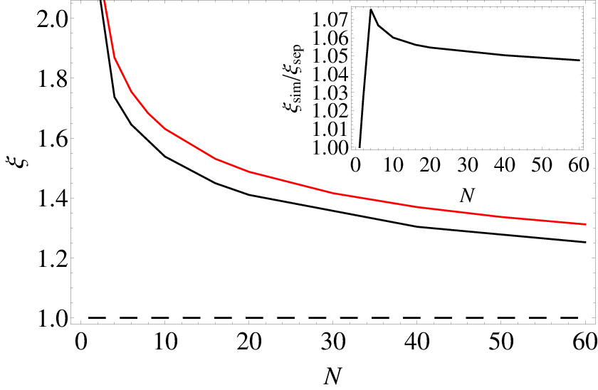
There still remains the issue of existence of a common input state optimal both for $\varphi$ and $\eta$ simultaneously. This fact is obvious for the single qubit case, $N=1$, as any equatorial qubit state is an optimal probe from the point of view of both parameters. For $N\geq 2$, however, this is no longer true. We have performed a numerical search which showed that when optimizing probe states from the point of view of estimating two-parameters simultaneously we face a trade-off and the optimal state for joint estimation depends on the weighting of importance between dephasing and phase estimation. Still, the observed trade-off is relatively small and shrinks with increasing $N$. We conjecture that for asymptotically large $N$ the discrepancy is vanishing and the simultaneous scheme performs as well as the separate one. This is presented in Fig. 4 where the average of estimation uncertainties of $\varphi$ and $\eta$ achievable when utilizing two-axis spin-squeezed states [45] normalized according to the asymptotic optimal performance of the separate schemes

is plotted. When the above quantity is calculated for separate and simultaneous schemes for $\eta=0.9$ the resulting discrepancy is maximal for $N=4$ when it achieves about $7.6\%$ and decreases with increasing $N$ going below $4.8\%$ for $N=60$ (see the inset). For smaller $\eta$ the discrepancy is even smaller although its maximum is attained for larger $N$. This numerics strongly suggests that asymptotically simultaneous scheme can perform as well as the separate one. The two-axis spin squeezed states used as an input probe here are parameterized using the squeezing parameter $\theta$ as $|\psi_{\theta}\rangle=e^{-\mathrm{i}\theta\left(J_{+}^{2}-J_{-}^{2}\right)}|j,j\rangle$ where $J_{+},\,J_{-}$ are standard angular momentum ladder operators and the dependence of optimal squeezing parameter as a function of $N$ is approximately $\theta\sim N^{-0.9}$ when $\eta=0.9$. We have also checked the behavior of one-axis spin-squeezed states, recently used in quantum enhanced magnetometry [46, 47], which are defined as $|\psi_{\theta}\rangle=U_{\phi}^{SSS}e^{-\mathrm{i}\theta J_{x}^{2}}|j,j\rangle$, where $J_{x}$ is $x$ component of the angular momentum, $U_{\phi}^{SSS}=e^{iH\phi}$ denotes unitary transformation generated by operator $H=e^{\mathrm{i}\theta J_{x}^{2}}J_{z}e^{-\mathrm{i}\theta J_{x}^{2}}$ and $\phi=\frac{1}{4}\arctan\left[\frac{4\sin\theta(\cos\theta)^{N-2}}{1-[\cos(2\theta)]^{N-2}}\right]$. Surprisingly, we have found that such states give significantly worse results and do not allow to saturate the performance of the separate schemes.

These conclusions are therefore similar to the ones obtained in [20] where a different model assuming collective instead of uncorrelated dephasing was analyzed and again asymptotic possibility of performing optimal simultanous estimation of phase and the dephasing parameter has been demonstrated.