QCD for collider experiments
Abstract
These lectures are intended to provide the theoretical basis of describing high-energy particle collisions at a level appropriate to graduate students in experimental high energy physics. They are supposed to be familiar with quantum electrodynamics, the concept of Feynman rules, Feynman graphs and computation of the cross section in quantum field theory.
When you measure what you are speaking about and express it in numbers, you know something about it, but when you cannot express it in numbers, your knowledge is of a meagre and unsatisfactory kind.
Lord Kelvin
1 QCD as quantum field theory of the strong interaction
The Lagrangian of the quark-gluon field based on a non-abelian gauge symmetry was first proposed in Ref. [1] forty years ago. The paper discussed the advantages of the colour-octet picture. Since then an immense amount of research lead to a lot of interesting results and a deep understanding of the strong interaction based on this quantum field theoretical description of chromo-dynamics, QCD. Today we are convinced that QCD is the correct description of the strong interaction, yet we still lack a complete and satisfactory solution. In such a situation one may set two goals: (i) either an ambitious one: solve QCD, or (ii) a more pragmatic one: develop tools for modeling particle interactions in high energy collider experiments. In these lectures we go for the second one.
Our aim is to understand high-energy particle collisions quantitatively from first principles. Examples of such events recorded by the CMS experiment at the LHC are shown in Fig. 1. In these events kinematic characteristics of particles, such as energy and momentum, are collected. Analyzing many such events, we can produce distributions of kinematic variables, for instance, differential distribution of the inclusive jet cross section with respect to pseudorapidity, . There is a long way from the QCD Lagrangian to making predictions for such distributions, full of difficulties. I clearly do not expect students in high energy experimental physics to be able to solve those difficulties. Instead I would like to explain the consequences of solving the difficulties, because an incomplete understanding of these consequences can easily lead to false interpretation of correct measurements.


1.1 The QCD Lagrangian
The quantum field theory (QFT) of the strong interactions is a part of the Standard Model (SM) of elementary particle interactions. The SM is based upon the principle of local gauge invariance. The underlying gauge group is
where c stands for “colour”, L for “left” (or “weak isospin”) and Y for “hypercharge”. As we concentrate on QCD, which is based on gauge symmetry, we can write the Lagrangian as
| (1) |
where
| (2) |
while the electroweak sector (based on the symmetry) act as sources. In Eq. (2) is the classical Lagrangian, while is the gauge-fixing term. The last piece is the ghost Lagrangian, absent if we use physical gauges, which will be our choice.
To find the classical Lagrangian, one starts with the Lagrangian of free Dirac fields,
| (3) |
where the matrices satisfy the Clifford algebra,
| (4) |
The matter field content is dictated by the electroweak sector. The fermion fields are called quark fields: with masses and , where is the number of different flavours. The quark fields also have an additional degree of freedom: colour, labelled by , that can take values, . The precise matter content is shown in Table 1.
| 1 | 2 | 3 | 4 | 5 | 6 | |
|---|---|---|---|---|---|---|
| u | d | s | c | b | t | |
| MeV | MeV | MeV | 1.2 GeV | 4.2 GeV | 172.6 GeV |
If we apply a transformation , with
where , then the Lagrangian of free Dirac fields remains invariant, . The are matrices that constitute the fundamental representation of the generators (called colour-charge operators), which satisfy the Lie algebra:
| (5) |
For the matrices are the Gell-Mann matrices (see \eg[2]).
Next we ask the question if we can make invariant under local transformations. The answer is yes, we can through the following steps:
- 1.
Introduce coloured vector field with the following transformation property under transformations:
where .
- 2.
Replace with . This covariant derivative transforms the same way as the quark field .
- 3.
Introduce a kinetic term
with the non-abelian field strength given by
so the Lagrangian contains cubic and quartic terms of the gauge field.
The constants are the structure constants of the Lie algebra. The structure constants are completely antisymmetric and are related to the adjoint representation of the generators by .
Thus we find that the gauge boson field, called gluon field, is a consequence of the local (gauge) invariance. The classical Lagrangian of QCD is a sum of interacting Dirac Lagrangians for spin 1/2 fermion fields and a Lagrangian of a gauge field,
| (6) |
where
| (7) |
The gluon field is also coloured and self-interacting. In fact, these self-interactions are the sources of the main difference between QED and QCD. We shall see that as a result, QCD is a ‘perfect theory’ in the sense that it is asymptotically free. Furthermore, among quantum field theories in dimensions only non-Abelian gauge theories are asymptotically free (see discussion after Eq. (21)). It is also plausible that the self-interactions are the sources of colour confinement, \iethe colour neutrality of hadrons, but we do not have a proof based on first principles.
It is clear that there is an unprecedented large number of degrees of freedom we have to sum over when computing a cross section:
- 1.
spin and space-time as in any field theory, not exhibited above,
- 2.
flavour, which also appears in electroweak theory, and colour, which is specific to QCD only.
As a result computations in QCD are rather cumbersome. During the last two decades a lot of effort was invested and great progress was made to find “simple” ways of computing QCD cross sections and to automate the computations.
Exercise 1.1
Show that in QED the covariant derivative transforms the same way as the field itself, i.e., if then , where .
Exercise 1.2
Show that in QED
where .
Exercise 1.3
Show that the generators of a special unitary group are traceless and hermitian.
Exercise 1.4
The generators in the fundamental representation of SU(2) are the Pauli matrices divided by two:
The adjoint representation of a group is defined as
Compute the generators in the adjoint representation of SU(2).
We define the constant for a representation by the condition
Compute this constant from the explicit form of the fundamental () and the adjoint () representation.
The quadratic Casimir of a representation is defined by
Compute the quadratic Casimir in the fundamental () and the adjoint () representation of using the explicit form of the representation matrices.
Exercise 1.5
Show that in SU(N) gauge theories
Exercise 1.6
Show that transforms according to the adjoint representation of SU(N):
1.2 Feynman rules
The Feynman rules can be derived from the action,
In this decomposition contains the terms bilinear in the fields and does all other terms, called interactions. The gluon propagator is the inverse of the bilinear term in . In momentum space we have the condition (we suppress colour indices as these terms are diagonal in colour space)
| (8) |
However,
| (9) |
which means that the inverse does not exist, the matrix is not invertible. We can exploit gauge invariance to rewrite the classical Lagrangian in a physically equivalent form (action remains the same) such that exists, which is called gauge fixing. This amounts to imposing a constraint on by adding a term to the Lagrangian with a Lagrange multiplicator (like in classical mechanics). For example, the covariant gauges are defined by requiring for any . Adding
to , the action remains the same. The bilinear term becomes in this case
with inverse
Of course, physical results must be independent of . It is customary to choose (called covariant Feynman gauge).
In covariant gauges unphysical degrees of freedom (longitudinal and time-like polarizations) also propagate. The effect of these unwanted degrees of freedom is cancelled by the ghost fields (coloured complex scalars with Fermi statistics). We do not elaborate the details of these fields as the unwanted degrees of freedom and the ghost fields can be avoided by choosing axial (physical) gauges, which is our choice. The axial gauge is defined with an arbitrary, but fixed vector , different from :
which leads to
Since , we have:
Thus, only 2 degrees of freedom propagate (transverse ones in the rest-frame). A usual choice is , called light-cone gauge. The price we pay by choosing this gauge instead of a covariant one is that the propagator looks more complicated and it diverges when becomes parallel to . In this gauge
with
| (10) |
where is the polarization vector of the gauge field (photon in QED, gluon in QCD).
1.3 Feynman rules for QCD
Propagators (Feynman’s ‘’-prescription is assumed, but not shown):
gluon propagator:
![[Uncaptioned image]](1608.02381v1/gluonpropagator.png)
quark propagator:
![[Uncaptioned image]](1608.02381v1/quarkpropagator.png)
ghost propagator:
![[Uncaptioned image]](1608.02381v1/ghostpropagator.png)
(not needed in physical gauges)
Vertices:
quark-gluon:
![[Uncaptioned image]](1608.02381v1/quarkgluonvertex.png)
three-gluon:
![[Uncaptioned image]](1608.02381v1/threegluonvertex.png)
four-gluon:
![[Uncaptioned image]](1608.02381v1/fourgluonvertex.png)
ghost-gluon: (not needed in physical gauges).
![[Uncaptioned image]](1608.02381v1/ghostgluonvertex.png)
The four-gluon vertex differs from the rest of the Feynman rules in the sense that it is not in a factorized form of a colour and a tensor factor. This is an inconvenient feature because it prevents the separate summation over colour and Lorentz indices and complicates automation. We can however circumvent this problem by introducing a fake field with propagator
![[Uncaptioned image]](1608.02381v1/fakepropagator.png)
that couples only to the gluon with vertex
![[Uncaptioned image]](1608.02381v1/fakegluonvertex.png)
.
We can check that a single four-gluon vertex can be written as a sum of three graphs. This way the summations over colour and Lorentz indices factorize completely, which helps automation and makes possible for us to concentrate on the colour algebra independently of the rest of the Feynman rules.
Finally, we have to supply the following factors for incoming and outgoing particles:
Exercise 1.7
Show that the four-gluon vertex can be written as a sum of three graphs, with the help of the fake field such that in each graph the colour and Lorentz indices are factorized:
![[Uncaptioned image]](1608.02381v1/fourgluonresolution.png)
1.4 Basics of colour algebra
Examining the Feynman rules, we find that there are two essential changes as compared to QED. One is that there is an additional degree of freedom: colour. The second is that there are new kind of couplings: the self couplings of the gauge field. We now explore the effect of the first.
In order to see how to treat the colour degrees of freedom, we set to one all but the colour part of the Feynman rules and try first to develop an efficient technique to compute the coefficients involving the colour structure. This is possible because the colour degrees of freedom factorize from the other degrees of freedom completely. We use the following graphical representation for the colour charges in the fundamental representation:
![[Uncaptioned image]](1608.02381v1/Ta.png)
.
The normalization of these matrices is given by Tr
![[Uncaptioned image]](1608.02381v1/normalization.png)
. The usual choice is , but is also used often. We shall use both.
In the adjoint representation the colour charge is represented by the matrix that is related to the structure constants by
![[Uncaptioned image]](1608.02381v1/Fabc.png)
where with are matrices which again satisfy the commutation relation (5). The graphical notation in the adjoint representation is not unique. For the matrix we assume an arrow pointing from index to , opposite to which we read the indices of (similarly as for the matrices ). On the structure constants the indices are not distinguished, therefore arrows do not appear. However, these are completely antisymmetric in their indices, therefore, the ordering matters. By convention, in the graphical representation, the ordering of the indices is counter-clockwise. The representation matrices are invariant under transformations.
The sums and Tr have two free indices in the fundamental and adjoint representation, respectively. These are invariant under transformations, therefore, must be proportional to the unit matrix,
which is depicted graphically as
![[Uncaptioned image]](1608.02381v1/casimirs.png)
.
Here and are the eigenvalues of the quadratic Casimir operator in the fundamental and adjoint representation, respectively. In the familiar case of angular momentum operator algebra (), the quadratic Casimir operator is the square of the angular momentum with eigenvalues . The fundamental representation is two dimensional, realized by the (half of the) Pauli matrices acting on two-component spinors, when and . In the adjoint representation and . Below we derive the corresponding values for general .
The commutation relation (5) can be represented graphically by
![[Uncaptioned image]](1608.02381v1/commutator.png)
.
Multiplying this commutator first with another colour charge operator with summing over the fermion index and then taking the trace over the fermion line (\iemultiplying with ) we obtain the resolution of the three-gluon vertex as traces of products of colour charges:
![[Uncaptioned image]](1608.02381v1/threegluonresolution.png)
We now show some examples of how one can compute the colour algebra structure of a QCD amplitude, in particular we will also find an explicit value for and . Taking the trace of the identity in the fundamental and in the adjoint representation we obtain
![[Uncaptioned image]](1608.02381v1/Trta.png)
![[Uncaptioned image]](1608.02381v1/TrFa.png)
,
respectively. Then, using the expressions for the fermion and gluon propagator corrections, we immediately find
![[Uncaptioned image]](1608.02381v1/qgloop.png)
![[Uncaptioned image]](1608.02381v1/ggloop.png)
, .
The generators are traceless,
![[Uncaptioned image]](1608.02381v1/qloop.png)
![[Uncaptioned image]](1608.02381v1/gloop.png)
, .
We can now find the value of as follows. On the one hand we know that
![[Uncaptioned image]](1608.02381v1/CFNc.png)
while on the other, the left hand side is also equal to . Thus
Analogously one can find
As the colour factors and depend on , their measurement gives information on the number of colours. The experiments of the Large Electron Positron collider measured the values of the colour factors based on fits of theoretical predictions [3] to four-jet angular distributions that are sensitive to both and . The result of the simultaneous measurement of the colour factors and the strong coupling by the OPAL collaboration is shown in Fig. 2 [4]. The values corresponding to are marked with the star, just in the middle of the confidence-ellipses.

The expression is invariant under transformations, therefore has to be expressible as a linear combination of and (the third combination of Kronecker ’s is not possible, the direction of arrows do not match). The two coefficients can be obtained by making contractions with and . Thus we obtain the Fierz identity,
or graphically:
![[Uncaptioned image]](1608.02381v1/fierz.png)
.
These graphical rules help in computing colour sums easily. Nevertheless, nowadays computer algebra codes make computation of colour sums an automated procedure. For instance, you may try In[1]:= Import["http://www.feyncalc.org/install.m"] in your Mathematica session to see one solution.
Exercise 1.8
Consider the process . Compute the color structures that appear in the squared matrix element.
Exercise 1.9
Try using the Fierz identity to obtain
![[Uncaptioned image]](1608.02381v1/qloopgg.png)
.
Exercise 1.10
Determine the color factors ,, in the following equations:
![[Uncaptioned image]](1608.02381v1/vertexA.png)
, ![[Uncaptioned image]](1608.02381v1/vertexB.png) ,
, ![[Uncaptioned image]](1608.02381v1/vertexC.png) .
.
1.5 Are we done?
We now have the Feynman rules with colour and the rest factorized, and we gained some insight how to perform the colour algebra. Thus it seems that we are in the position to compute the cross section of any process up to the desired accuracy in perturbation theory (PT), just as we can do in QED. So it may appear that conceptually we are done. Well, we are going to see big surprises!

The first conceptual challenge is due to a phenomenological observation. In QED, PT is applicable because the elementary excitations of the quantum fields, the electrons and photons, can be observed as stable, free particles. Thus asymptotic states are parts of the physical reality. On the contrary, free quarks and gluons (usually called simply partons) have never been observed in nature. This experimental fact can be reformulated saying that the probability of observing a final state with any fixed number of on-shell partons is zero. This negative result has been turned into the principle of ‘quark confinement’. Thus it is questionable whether a QFT of quark and gluon fields can describe the observed world of particles where in addition to leptons only hadrons have been found. In fact, a main research project at the LEP was to find an answer to this question in a well controlled quantitative manner. It turned out that the answer is positive if we make an assumption that we cannot prove from first principles:
The result of a low-order perturbative computation in QCD is an approximation to sufficiently inclusive hadronic cross section if (i) the total centre-of-mass energy of partons is much larger than the mass of quarks, , and (ii) is far from hadronic resonances and thresholds.
We shall define precisely what ‘sufficiently inclusive’ means later. Predictions made on the basis of this assumption agree with measurements (e.g. made at LEP) within the expected accuracy of the prediction, which we are to define also later.
Based on this assumption, it makes sense to make predictions with quark and gluon asymptotic states. However, in QCD the complexity of the Feynman rules will make higher order computations prohibitive. Indeed, the largest effort in QCD computations during the past 20 years went into devising ever more efficient methods to decrease the algebraic complexity of the computations. This research is driven by the observation that the QCD Lagrangian is highly symmetric, which has to be reflected in the final results. Thus the complications somehow appear mainly because with our rules we artificially introduce complications at intermediate steps of the computations, which cancels to large extent in the final formulae. Learning about the symmetries of QCD is interesting and useful not only for technical purposes, so let us make an inventory of those.
1.6 Symmetries of the classical Lagrangian
The symmetries can be grouped into two large categories: exact symmetries and approximate ones. Space-time symmetries are exact. These consist of invariance against continuous transformations: translations and Lorentz-transformations (rotations and boosts). In addition is invariant under scale transformation:
and conformal transformations, which we do not detail here. The Lagrangian is also invariant under charge conjugation (C), parity (P) and time-reversal (T), in agreement with observed properties of strong interactions (C, P and T violating strong decays are not observed).
We already discussed exact symmetry in colour space: local gauge invariance. In addition to the classical Lagrangian of Eq. (6), there exists additional gauge invariant dimension-four operator, the -term:
that violates P and T. As experimentally , we set in perturbative QCD.
Another interesting feature of is that it is almost supersymmetric. For one massless flavour
which is very similar to the Lagrangian of supersymmetric gauge theory,
The only difference is that the quark transforms under the fundamental, while the gluino under the adjoint representation of the gauge group.
An important approximate symmetry of the classical Lagrangian is related to the quark mass-matrix. Let us introduce the quark flavour triplet
with each component being a four-component Dirac spinor, and the combinations
| (11) |
The latter are projections:
It follows from Clifford-algebra that . We define . Using , we find that are eigenvectors of with eigenvalues:
From the definition of the Dirac adjoint, , we obtain . Thus the quark sector of the Lagrangian can be rewritten in terms of the chiral fields :
This decomposition would not work if the gluon field in the covariant derivative were not Lorentz-vector. In this chiral form the left- and right-handed fields decouple, so the Lagrangian is invariant under separate transformations for the left- and right-handed fields, \ieunder , hence it is called chiral symmetry. Indeed, if , then under the transformation
remains invariant. This symmetry is exact if the quarks are massless. The group elements can be parametrized using real numbers (, ),
where the matrices represent the generators of the group ( matrices). The transformations , , acting as , form a vector subgroup . The transformations , acting as , however, do not form an axial-vector subgroup because
This chiral symmetry is not observed in the hadron spectrum. Therefore, we assume that vacuum has a non-zero VEV of the light-quark operator,
a chiral condensate that connect left- and right-handed fields,
The condensate breaks chiral symmetry spontaneously to . This remaining symmetry explains the existence of good quantum numbers of isospin and baryon number, as well as the appearance of massless mesons, the Goldstone bosons. As non-zero quark masses violate the chiral symmetry, which is broken spontaneously, the Goldstone bosons are not exactly massless. Thus we have natural candidates for the Goldstone bosons: we can identify those with the pseudoscalar meson octet. In practice, we assume exact chiral symmetry and treat the quark masses as perturbation. This procedure leads us to chiral perturbation theory (PT) [5], which is capable to predict the (ratios of) masses of light quarks [6, 7], scattering properties of pions [8] and many more. Although, PT is a non-renormalizable QFT, it can be made predictive order by order in PT if the measured values of sufficiently many observables are used to fix the couplings of interaction terms at the given order.
The QCD Lagrangian was written forty years ago. Since then many attempts were tried to solve it and mature fields emerged that aim at solving the theory in a limited range of physical phenomena. For instance, PT is a PT that uses low-energy information (in the MeV range) to explain the world of hadrons and masses of light quarks. In the same energy range non-perturbative approaches, notably lattice QCD and sum rules have been developed for the same purpose. By now it is possible to explain the light hadron spectrum from first principles using lattice results [9]. The main goal at colliders, our focus in these lectures, is different. We shall prove that PT can give reliable predictions for scattering processes at high energies, which is the topic of jet physics.
We have seen that the classical QCD Lagrangian shows many interesting symmetry properties that can be utilized for (i) easing computations, (ii) checking results, (iii) hinting on solving QCD. We shall see that some of these symmetries are violated by quantum corrections, which leads to important physical consequences. In QCD an important example is scaling violations. Another example is the axial anomaly which provides strong constraints on possible QFT’s, but it is discussed within the electroweak theory usually.
1.7 What is scaling?
Let us consider a dimensionless physical observable that depends on a large energy scale . Large means that is much bigger than any other dimensionful parameter, for instance, masses of quarks. Thus we assume that these other dimensionful parameters can be set zero.11 1 We shall study the validity of this assumption in the next subsection. Classically, dim and, since is dimensionful, it follows that . So constant, which is called scaling.
In these lectures we do not have room for a complete description of ultraviolet (UV) renormalization of QCD. We simply state that in a renormalized QFT depends also on another scale, the renormalization scale . So
need not be a constant. This is called scaling violation. The first term in parenthesis is the only dimensionless combination of and . However, is arbitrary. If depended on , then its value could not be predicted. For simplicity from now on we drop the subscript “R” from . As is an arbitrary, un-physical parameter (the classical Lagrangian did not contain ), we expect that measurable (physical) quantities cannot depend on it, which is expressed by the renormalization group equation (RGE):
We can simplify this equation a bit by introducing the new variable and the function ,
| (12) |
Then the RGE becomes
| (13) |
To present the solution of this partial differential equation, we introduce the running coupling , defined implicitly by
| (14) |
where is an arbitrarily fixed number. The derivative of Eq. (14) with respect to the variable gives
The derivative of Eq. (14) with respect to gives
from which it follows that
It is now easy to prove that the value of for , solves Eq. (13):
and
It then follows that the scale-dependence in enters only through , and we can predict the scale-dependence of by solving Eq. (14), or equivalently,
| (15) |
So far our analysis was non-perturbative. Assuming that PT is applicable, which we shall discuss at the end of this subsection, we may try to solve Eq. (15) in PT where the -function has the formal expansion:
| (16) |
The first four coefficients are known from cumbersome computations [10]
| (17) |
The first two coefficients in the expansion of the function are independent of the renormalization scheme. The second two coefficients in Eq. (17) are valid in the renormalization scheme.22 2 As we have not gone through the renormalization procedure, we cannot define precisely what we mean by ‘renormalization scheme’. Various schemes differ by finite renormalization of the parameters and fields in the Lagrangian.
Another often used convention is
| (18) |
where and , thus .
If is small we can truncate the series. The solution at leading-order (LO) accuracy is
| (19) |
which gives as a function of if both are small; is a number to be measured. We observe that:
| (20) |
This behaviour is called asymptotic freedom. The sign of (positive for QCD) plays a crucial role in establishing whether or not a theory is asymptotically free. If it is, then the use of PT is justified: the higher , the smaller the coupling. The coefficient is easiest to compute in background field gauge [11] where only three graphs contribute, the quark and gluon loops:
| (21) |
and a similar ghost loop. The contribution of the quark loop is negative , while that of the gluon+ghost loop is positive . (We knew the colour factors immediately, only the coefficients have to be computed!) The net result is positive up to in QCD. In 2004 D.J. Gross, H.D. Politzer and F. Wilczek were awarded the Nobel prize for their discovery of asymptotic freedom in QCD [12, 13].
Clearly, it is the gluon self-interaction that makes QCD perfect in PT. In QED, in the absence of photon self-interaction, , hence the coupling increases with energy, but remains perturbative up to the Planck scale ( GeV) where we expect that any known physics breaks down.
Asymptotic freedom gives rationale to perturbative QCD, but we shall see that LO accuracy is not enough. The analysis is also simple at next-to-leading order (NLO):
is then given implicitly by the equation
which can be solved numerically.
Using the formula for the sum of the geometric series, and recalling Eq. (19), we find that the running coupling sums logarithms,
The NLO term gives logarithms with one power less
in each term.

1.8 Measuring
We know if is known. We therefore, have to measure at some scale . The perturbative solution of the renormalization group equation (RGE, Eq. (13)) is never unique. The difference between two solutions at is suppressed by , i.e. at . Nevertheless, this difference can lead to significant difference in if and are far from each other, which is important in present day precision measurements. Therefore, the scale is chosen to be because GeV is not far from the scales where is used in current experimental analyses. In Figs. 4 and 5 we show the present status of measurements from Ref. [14].

Another approach to solving the RGE is to introduce a refence scale by
The scale indicates where the coupling becomes strong. The following exercise is to explore the characteristics of this choice.
Exercise 1.11
The running of the strong coupling constant is given by Eq. (12). The perturbative expansion of the QCD beta function is given by Eq. (18) with . Determine (i) the expression for the coupling constant in leading order (, ) and the corresponding scale (see below) (ii) the expression for the coupling constant in next-to-leading order (, ) and the corresponding scale (see below).
Hints:
- 1.
Solve the differential equation for ; you’ll get an integration constant.
- 2.
Express your result in the form
where is a constant.
- 3.
Solve the differential equation using
- 4.
This time the solution cannot be solved for analytically. One can nevertheless find an approximate solution by expanding in . The constant is not equal to the one in the first part of this exercise.
- 5.
Cast your equation for into the form
with a suitable choice of .
- 6.
Expand the right hand side of your equation in and keep only the first order term. Use the expansion
1.9 Quark masses and massless QCD
Quark masses are parameters of like the gauge coupling, which need to be renormalized. In QED the electron mass is measured in the laboratories at (classical limit). We cannot similarly isolate a quark at (at low scale quarks are confined). Instead, we can perform a similar RGE analysis as with . For simplicity we assume one quark flavour with mass , which is yet another dimensionful parameter, so the RGE becomes:
| (22) |
where is called the mass anomalous dimension and the minus sign before is a convention. In PT we can write the mass anomalous dimension as
with known coefficient up to . At NLO accuracy we need only and . As is dimensionless, the dependence on the dimensionful parameters has to cancel
| (23) |
The difference of Eqs. (22) and (23) gives the dependence of on :
| (24) |
This equation is solved by introducing the running mass (in addition to the running coupling) obeying
| (25) |
Exponentiating, changing integration variable from to and using the definition of the function, we obtain
| (26) |
which means that asymptotically free QCD is a massless theory at asymptotically large energies. At LO in PT theory the solution of (26) is given by
where we introduced the abbreviation . At NLO the solution becomes
In terms of the running coupling and mass, is a solution of Eq. (24), proven similarly as being the solution of Eq. (13). Expanding around , we obtain
| (27) |
We see from Eq. (27) that derivative terms are suppressed by factors of at large . From the dependence of on we can conclude that the effect of mass is suppressed at high by its physical dimension and also by its anomalous dimension, which justifies the assumption about negligible quark masses. The expansion in Eq. (27) has a deeper consequence. The dimensionless observable may depend on that can become large when is large. If we want to avoid such large logarithms, we should consider physical observables (that is physically measurable quantities) that have a finite zero-mass limit.
2 Predictions in perturbative QCD

In a typical collider experiment we collect collision events with something interesting in the final state. For instance, in searching for the Higgs boson, events with four hard muons such as in Fig. 6 are interesting. Counting the event rate of such events we obtain measured cross sections, which compare to theoretical predictions. Following our assumption about the use of low-order perturbative predictions in QCD, for such comparisons we need predictions for cross sections with partons. We start with the simplest possible case when partons appear only in the final state: electron-positron annihilation into hadrons (and possibly other particles).
Let us consider a measurable quantity , that has non-vanishing value for at least partons in the final state. At LO accuracy the basic formula for the differential cross section in is
| (28) |
where contains non-QCD factors (\egthe flux factor), is the phase space of particles, is a symmetry factor, is the squared matrix element (SME), and is the value of computed from the final state momenta. The integration is usually done by Monte Carlo integration and the hard part of the computation is to obtain the SME. In these lectures we can compute hardly any SME explicitly. Fortunately, there are freely available computer programs [15, 16, 17, 18, 19] that can be used to check the formulae. Even more, these programs can often be used to obtain the cross sections at LO accuracy, too.
We now use Eq. (28) to make predictions for the cross section of electron-positron annihilation into hadrons.
2.1 ratio at lowest order
The leading-order (LO) perturbative contribution to the cross section is . The calculation is like in the case of , supplemented with colour and fractional electric charge of . The colour diagram is a loop in the fundamental representation which corresponds to a factor as we have seen in the previous chapter. While the annihilation into contains only one flavour in the final state, quarks can have three, four or five flavours depending on the centre-of-mass energy.33 3 The sixth flavour, the top is so heavy that it cannot contribute at CM energies attained in experiments so far. We have, therefore, to sum over all possible flavours which can appear. The ratio of the two cross sections is thus given by
| (29) |
where and . If we consider only the up, down, strange and charm quarks . Considering also the bottom quark . This step-wise increasing behavior of the -ratio was observed (see Fig. 7), providing an experimental confirmation of the existence of 3 families of quarks and of the gauge-symmetry of QCD with .

According to our basic assumption, pQCD cannot give predictions for the resonances in Fig. 7. However, there is one exception, the impressive peak. The LO prediction uses the cross section for the process. A process has only a single free kinematic variable, the scattering angle . In the full SM the differential cross section for electron-positron annihilation into a massless and colourless fermion pair is obtained from the square of a single Feynman graph, , as
![[Uncaptioned image]](1608.02381v1/Rtree.png)
| (30) |
where we neglected terms that vanish at centre-of-mass energy , or after integration. , and denote the fractional charge, axial-vector and vector electroweak couplings of the fermions and is a number. Well below the peak the propagator becomes negligible and the total cross section is obtained by integrating over the scattering angle and we find the LO prediction , where . On the peak the same integration results in . Then we can make prediction for the hadronic ratio at LO accuracy by simply counting the contributing final states and relating their total charge factors to that of the muon and find away from the peak and on the peak. The factor three is due to the three colours of quarks. Considering five quark flavours, \ie, we find and . We have seen on Fig. 7 that 11/3 is fairly close to the measured value away from the peak. The measured value of at LEP is [20]. The LO prediction works amazingly well. The 3.5% difference is mainly due to QCD radiation effects that we call NLO corrections. Our next goal is to understand the origin of those corrections.
Exercise 2.1
Derive the result in Eq. (30) (at least below the peak, where you consider only photon intermediate state) and integrate it over .
Exercise 2.2
Use Mathematica and the Package Tracer.m (or FORM) to compute the following traces:
2.2 Ultraviolet renormalization of QCD
The strong coupling is rather large as compared to the other couplings in the SM, and as a result, the QCD radiative corrections are also large. Therefore, it is always important to compute at least the NLO accuracy, but if possible, even higher order corrections.44 4 There is even a more severe reason that we shall discuss later.
The computation of QCD radiative corrections is technically quite involved and a good organization of the calculations is very important. Thus, first we introduce some notation. The tensor product of the ket vectors denotes a basis vector in colour and helicity space, is a state vector of final-state particles in colour and helicity space. The amplitude for producing final-state particles of colour , spin , momentum is
| (31) |
(), so
| (32) |
The loop expansion in terms of the bare coupling, \iethe coupling that appears in the classical Lagrangian, is:
| (33) |
where , is the dimensional regularization scale, introduced to keep dimensionless in dimensions. The exponent in the prefactor takes account of the power of at LO, the loop-expansion is an expansion in the strong coupling . For instance, for , while for . The tree amplitude is finite, while the one-loop correction is divergent in dimensions, which is manifest in terms of and poles if dimensional reglarization is used. These poles have both ultraviolet (UV) and infrared (IR) origin.
The UV poles can be removed by multiplicative redefinition of the fields and parameters in the Lagrangian, systematically order by order in PT. This is a hard task even at one loop, but presently known up to four loops [21] – a truly remarkable computation! It turns out that when computing scattering amplitudes in massless QCD at one-loop accuracy, the renormalization amounts to the simple substitution
| (34) |
with . Note that on the left of this substitution is the dimensional regularization scale to keep dimensionless, while on the right is the renormalization scale. We discussed in Sect. 1.8 when we extract from measurements, we have to define . The dimensional regularization scale turns into the renormalization scale through the substitution (34).
Why does the substitution (34) work? Each Feynman graph consists of vertices with propagators connecting those and external lines. Moreover,
-
each vertex receives a factor (or for quartic vertex) and factors of , () for each field connected to the vertex,
-
each propagator of field receives a factor of ,
-
each external leg of field receives a factor of .
Thus the renormalization field factors cancel from each graph and only the charge renormalization () is needed in practice! This can be seen as a consequence of the fact that in massless QCD the only free parameter besides the gauge-fixing parameter is . The scattering amplitudes are physical, and any physical quantity has to be independent of , so the only remaining parameter, which the amplitudes may depend on, is the coupling. The renormalization factor is most easily computed in background field gauge, defined by
| (35) |
where is a background field and describes the quantum fluctuations on this background. It can be shown [11] that in this gauge the field and coupling renormalization factors are related by the Ward identity , and can be computed from loop insertions into the propagator shown in (21).
The simple substitution rule (34) for the coupling leads to a simple shift in the amplitude. As
we obtain for the renormalized amplitude
| (36) |
The renormalized theory is UV finite, yet is still infinite in dimensions, as it is divergent also in the infrared. After UV renormalization is achieved we can use dimensional regularization to regulate the amplitudes in the IR by continuing into (). The integrals that are scaleless in have mass dimension in dimensions. Therefore, in the massless limit all integrals can depend only on momentum invariants raised to a positive fractional power . We conclude that when all external invariants vanish, the continued integral must also vanish (“scaleless integrals vanish in dimensional regularization”).
For IR-safe observables these IR poles vanish and we can set at the end of the computations, and we obtain the UV finite, IR regularized SME that can be used to compute cross sections.
Exercise 2.3
Compute the contribution to the beta function from the fermion loop:
![[Uncaptioned image]](1608.02381v1/ZAfermion.png)
- 1.
Write down carefully the amplitude and compute the trace.
- 2.
The following types of integrals occur:
(37) Express these as linear combination of
(38) - 3.
Obtain from
(39) and find the divergent pieces.
The contribution to is the coefficient of the pole without the coupling factor.
2.3 ratio at NLO accuracy
This is by far the simplest example of computing QCD radiative corrections. As we saw in Sect. 2.1 it requires the total hadronic cross section that depends only on a single kinematic invariant, the total centre-of-mass energy . As a result, the emerging integrals in this computation can be evaluated exactly. Nevertheless, the complete computation is still too lengthy, and we shall be able to present the main step and filling the details is left to the student.
There are two kinds of corrections that contribute at NLO accuracy. One is the real correction, with an additional gluon in the final state, so the SME is computed from Feynman graphs as
, which gives an correction. The other kind of contribution
![[Uncaptioned image]](1608.02381v1/Rreal.png)
is the virtual correction, with an additional gluon providing a loop in the final state,
| .
![[Uncaptioned image]](1608.02381v1/Rvertex.png)
The real correction has three particles in the final state. The three-particle phase space has five independent variables: two energies and three angles. As we are looking for the total cross section, we integrate over the angles and use scaled two-particle invariants to write both the phase space and the SME. Momentum conservation implies . The complete real contribution to the total cross section is
| (40) |

This integral is divergent along the boundaries at , as well as in the point , so the singularities are in the IR parts of the phase space. As , the divergence occurs either when , which is called soft-gluon singularity, or when , which is called collinear singularity (the gluon is collinear to either of the quarks). The region of integration with the singular places is shown in Fig. 8.
To make sense of the integral, we use dimensional regularization, which amounts to the computation of the phase space and the SME in dimensions. The result is
| (41) | |||||
where (the exact form of this function will turn out to be irrelevant). The integrals can be evaluated exactly, but actually the Laurent-expansion around is sufficient,
| (42) |
The computation of the virtual correction is even more cumbersome due to the loop integral. We present only the result:
| (43) |
We now see that the sum of the real and virtual contribution is finite in , so for the sum we can set and find the famous correction: . The correction is the same for .
Actually there is a much easier way of computing the radiative corrections to the total cross section from the imaginary part of the hadronic vacuum polarization, using the optical theorem (). The state of the art is at [22]. The result of the computation at next-to-next-to-leading order (NNLO) accuracy,
| (44) |
satisfies the RGE to order . The coefficients , , suggest that the perturbation series is convergent. Our more complicated way of computing is instructive for our studies in the next section.
The predictions at the first three fixed orders in PT for are shown in Fig. 9. The ratio at LO accuracy does not depend on the strong coupling, hence it is independent of the scale. The figure is meant to show the general pattern of QCD predictions which, with the exception of the ratio, depend on the scale already at LO. The NLO curve shows the typical feature of LO predictions: it depends on the renormalization scale in a monotonically decreasing way. As this scale is unphysical, in principle, its value can be arbitrary. Thus the prediction at LO is in general only an order of magnitude indication of the cross section, but not a precision result. (In the case of the hadronic ratio the QCD corrections are actually quite small as compared to many other QCD cross sections and the precision is actually better than usual.) As a result, if we want to make reliable predictions in pQCD, the NLO accuracy (NNLO for ) is absolutely necessary unless we have some way to fix the scale.
However, there is no theorem that tells us the proper scale choice. The usual practice is to set the scale at a characteristic physical scale of the process. A reasonable assumption that the strength of the QCD interaction for a process involving a momentum transfer is given by , so is the proper scale choice, to minimize logarithmic contributions in higher-order terms. For instance, in case of electron-positron annihilation the total centre-of-mass energy is the usual choice, while for a jet cross section in proton-proton collisions the transverse momentum of the jet55 5 We discuss jets in the next section. is used. The application of this recipe appears clear as long as there is only one hard scale in the process. In the state of the art computations there are complex processes with several scales and it is not obvious which one to choose. For instance, in vector boson hadroproduction in association with jets () [23], in addition to the transverse momentum of the vector boson there are the transverse momenta of the jets. In this example, the choice was found to result in a badly behaving perturbation series with corrections driving the distribution of the second hardest jet at NLO accuracy even unphysically negative for and GeV at the LHC. Choosing a dynamical scale, set event by event, appears a better choice. For instance, half the total transverse energy of the final-state particles (both QCD partons and leptons from the decay of the vector boson), , leads to much milder scale dependence and a similar shape of the distributions at LO and NLO accuracies.
There are suggestions on making educated guesses for the best scale. Among those are the principle of fastest apparent convergence (FAC), that of minimal sensitivity (PMS), or the BLM scale choice [24, 25, 26], beyond the scope of these lectures. The experience is that in hadron collisions there is no choice that works well for any process and it is best to choose a dynamical scale chosen by examining the process.
As there is no unique scale, the standard procedure is to choose a default scale , related to the typical momentum transfer in the process, and to assign a theoretical uncertainty by varying the scale within a certain range around the default choice . The usual range is between half and twice the default choice. However, this is again an indication only of the scale uncertainties and there is no mathematical theorem that states this procedure yields the true theoretical uncertainty due to neglected higher order terms. In order to have a measure on the effect of neglected higher orders, \ieto understand the reliability of the assigned theoretical uncertainty one has to compute the NNLO corrections. The latter are very demanding computations both technically and numerically and predictions at NNLO accuracy for some fairly simple processes, with one or two final-state particles in the prediction at LO, constitute the state of the art of pQCD.
Exercise 2.4
Show that the -dimensional three-particle phase space for can be expressed in terms of the Lorentz-invariants
where is the measure of the hypersurface element in dimensions, . Hints:
- 1.
The -dimensional volume measure in spherical coordinates is recurisvely given by
- 2.
Show that
where is the angle between and .
Exercise 2.5
Let . Using the previous exercise, compute the real correction to the process given in Eq. (42). Hint: Transform the triangular integration region into the unit square and evaluate the (Euler ) functions.
3 Jet cross sections
In the first two sections we established our theoretical playground to make predictions for hadronic cross sections. Based on RGE analysis we showed that PT can only be fully consistent in an asymptotically free QFT, like QCD. We found that predictions can be made only for those quantities that remain finite in the limit of vanishing masses of light quarks. We computed the radiative corrections for such a quantity, the total hadronic cross section in electron-positron annihilation. We found that at intermediate steps of the computations there are singular contributions of two types: of UV and IR origin. The UV singularities can be removed by renormalization, and the remaining IR ones can be regularized in dimensional regularization where IR singularities appear as poles. When adding all contributions, these poles cancel and we obtain the finite correction after setting . Our question in this section is whether there are more exclusive observables than the totally inclusive one for which this procedure can be applied.


It is clear from experiments that typical final states have structures. For instance, Fig. 10 shows two events, one with two and the other with three sprays of hadrons, called hadron jets. If we count the relative number of events with two, three, four jets, an interesting pattern emerges:
# of events with 2 jets : # of events with 3 jets : # of events with 4 jets : : .
Recalling our basic assumption and Fig. 3 we find that jets reflect the partonic structure of the events. We now use our pQCD formalism to describe these structures theoretically. For this purpose, we need a function of the final state momenta that quantifies the structure of the final state in some ways (we give examples below). This function is called jet function.
Let us consider again the process hadrons. If we are not interested in the orientation of the final state events, we can average over the orientation and find that the SME has no dependence on the parton momenta. Then the two-particle phase space is , and contribution of the process to the cross section is
| (45) |
which sets our normalization of . The two kinds of NLO corrections are
| (46) |
Contrary to the case of the total cross section, where , we cannot simply perform the integration analytically and combine the results, neither we can combine the integrands. The general method to deal with this problem is to regularize both with a properly chosen subtraction,
such that both terms are separately integrable in dimensions. This requires a special property of the jet function , called IR safety, expressed analytically as
| (47) |
Qualitatively IR safety means that the jet function is insensitive to an additional soft particle, or to a collinear splitting in the final state.
How can we construct such an approximate cross section? For this simple process we can follow the steps:
| (48) |
Then introduce the new variable , so that and
and substitute these into Eq. (48):
| (49) |
The term never becomes infinite, thus the approximate cross section
| (50) |
| (51) |
is a proper subtraction term that regularizes the real contribution in all of its singular limits in dimensions. Consequently, the difference can be integrated in any dimensions, in particular, we can set and integrate in numerically.
To obtain we integrate the two terms separately. For we change variables in the phase space to and , and find
| (52) |
We shall see that this factorization of the singular terms is universal. We can now perform the integration over the factorized one-particle phase space, independently of the jet function, and obtain the integrated subtraction term in the form with insertion operator
| (53) |
Comparing this integrated subtraction to Eq. (46), we see that the sum is finite if ,
| (54) |
and so can be integrated in dimensions.
3.1 Infrared safety
A natural question is if we can construct the approximate cross section
universally, \ieindependently of the process and observable. Our
presentation above suggests the affirmative answer. To understand how, we
have to study the origin of the singular behaviour in the SME. This
singularity arises from propagator factors that diverge
![[Uncaptioned image]](1608.02381v1/singularity.png)
In the collinear limit, and less singular terms (a factor of appears in the numerator factors). In the soft limit, and less singular terms. The gluon phase space is
so in the cross section we find logarithmic singularities in both the soft and the collinear limits: or . These are the IR singular limits. In dimensional regularization the logarithmic singularities appear as poles:
Thus, the singular behaviour arises at kinematically degenerate phase space configurations, which at the NLO accuracy means that one cannot distinguish the following configurations: (i) a single hard parton, (ii) the single parton splitting into two nearly collinear partons, (iii) the single parton emitting a soft gluon (on-shell gluon with very small energy). Then an answer to the question posed at the beginning of Sect. 3 is given by the Kinoshita-Lee-Nauenberg (KLN) theorem [27, 28]:
In massless, renormalized field theory in four dimensions, transition rates are IR safe if summation over kinematically degenerate initial and final states is carried out.
For the hadrons process, the initial state is free of IR singularities. Typical IR-safe quantities are (i) event shape variables and (ii) jet cross sections.
3.2 Event shapes

Thrust, thrust major/minor, C- and D-parameters, oblateness, sphericity, aplanarity, jet masses, jet-broadening, energy-energy correlation, differential jet rates are examples of event shape variables. The value of an event shape does not change if a final-state particle further splits into two collinear particles, or emits a soft gluon, hence it is (qualitatively) IR safe. As as example we consider the thrust , which is defined by
| (55) |
where is a three-vector (the direction of the thrust axis) such that is maximal. The particle three-momenta are defined in the centre-of-mass frame. is an example of the jet function . It is infrared safe because neither , nor replacing with change . At LO accuracy it is possible to perform the phase space integrations and
| (56) |
We see that the perturbative prediction for the thrust distribution is singular at . In addition to the linear divergence in there is logarithmic divergence, too. The latter is characteristic to events shape distributions. In PT at th order logarithms of in the form appear. These spoil the convergence of the perturbation series and call for resummation if we want to make reliable prediction near the edge of the phase space, for large values of where the best experimental statistics are available. Resummations of leading () and next-to-leading () logarithms are available for many event shape variables, but the discussion of this technique is beyond the scope of these lectures.
Exercise 3.1
Verify that as defined in Eq. (55) is infrared und collinear safe. What is the range of values that can take if (i) there are only two particles in the final state, or (ii) and all are distributed spherically?
3.3 Jet algorithms
Jets are sprays of energetic, on-shell, nearly collinear hadrons. The number of jets does not change if a final-state particle further splits into two collinear particles, or emits a soft gluon, hence it is again qualitatively IR safe. To quantify the jet-like structure of the final states jet algorithms have been invented. These have a long history with rather slow convergence. The reason is that the experimental and theoretical requirements posed to a jet algorithm are rather different. Experimentally we need cones that include almost all hadron tracks at cheap computational price. Theoretically the important requirements are IR safety, so that PT can be employed to make predictions and resummability, so that we can make predictions in those region of the phase space where most of the data appear.
For many years experimenters preferred cone jet algorithms (according to the ‘Snowmass accord’) [29]. These start from a cone seed (centre of the cone) in pseudorapidity () and azimuthal-angle () plane: (). We define a distance of a hadron track from the seed by . A track belongs to the cone if , with a predefined value for (usually 0.7). It turned out however, that (i) this is an IR unsafe definition and (ii) there is a problem how to treat overlapping cones, so the cone jet definition has been abandoned.
Theoreticians prefer iterative jet algorithms, consisting of the following steps. (i) First we define a distance between two momenta (of partons or hadron tracks) and a rule to combine two momenta, and into . (ii) Then we select a value for resolution and consider all pairs of momenta. If the minimum of is smaller than , then we combine the momenta and and start the algorithm again. If the minimum is larger than , then the remaining momenta (after the combinations) are considered the momenta of the jets, and the algorithm stops. The drawback of this algorithm is that it becomes very expensive computationally for many particles in the final state. This is not an issue in pQCD computations because according to our basic assumption there are only few partons, but a major problem for the final states in the detectors where hundreds of hadrons may appear in a single event.
At LEP theory won and the Durham (or ) algorithm was used. It was invented so that resummation of large logarithms could be achieved [30]. The distance measure is , where and the recombination scheme is simple addition of the four momenta, . The resolution parameter can take values in . The pQCD prediction contains logarithmically enhanced terms of the form , at any order, which has to be resummed if we want to use small value of , where we find the bulk of the data (see Figure 12). Predictions are available with leading- () and next-to-leading () logarithms (LL and NLL) summed up to all orders [30].
Figure 12 shows the fixed order LO and NLO predictions, as well as predictions where NLO and NLL are matched. The curve at NLO accuracy gives a good description of the measure data by the ALEPH collaboration [31], but only for . As , for smaller values of resummation is indispensable. The resummed prediction however, is not expected to give a good description at large because in the resummation formula only the collinear approximation of the matrix element is used. Matching the two predictions gives a remarkably good description of the data over the whole phase space.
At hadron colliders the algorithm needs modifications. First, instead of energy, the boost-invariant measure of hardness, transverse momentum is used to define the distance between tracks, where (distance in rapidity–azimuthal-angle plane), is a small positive real number, and we need a distance from the beam , too. Also, the algorithm needs modification because either or can be the smallest distance. If a is the smallest value, then and are merged, while if the smallest is a , then momentum becomes a jet momentum and is removed from the tracks to be clustered. We then call jet candidates with transverse momentum resolved jets. The merging rule may change as well. In the usual merging we add four-momenta, but another option is to add transverse momenta, , and add rapidities and azimuthal angles weighted, and , where the weight can be , , , or . Such a merging is boost invariant along the beam. The parameter plays a similar role as in electron-positron annihilation or the cone radius in the cone algorithms: the smaller , the narrower the jet.
The iterative -algorithm is infrared safe and resummation of large logarithmic contributions of the form and is possible, which is a clear advantage from the theoretical point of view. The logarithms are those of and/or , being the hard process scale. By taking sufficiently large in hadron-hadron collisions, we avoid such leading contributions from initial-state showering and the underlying event, so these terms are determined by the time-like showering of final-state partons (when the virtuality of the parent parton is always positive). Particles within angular separation tend to combine and particles separated by larger distance than from all other particles become jets. The algorithm assigns a clustering sequence to particles within jets, so we can look at jet substructure.
Nevertheless, at the TeVatron experiments the -algorithm did not become a standard for several reasons. The jets have irregular, often weird shapes as seen on Fig. 13(a) because soft particles tend to cluster first (even arbitrary soft particles can form jets). As a result there is a non-linear dependence on soft particles, energy calibration and estimating acceptance corrections are more difficult. The underlying event correction depends on the area of the jet (in plane). It was also very expensive computationally, so experimenters had a clear preference of cone algorithms.


The breakthrough occurred with Refs. [33, 34] where variants of the algorithm and an improved, fast implementation was introduced. The distance formula was modified to (). IR-safety is independent of , as well as NLL resummation of large logarithms. It was found that with (called anti--alogrihtm) particles close in angle cluster first, which results in regular cone-like shapes as seen on Fig. 13(b) without using stable cones. As a result it became the standard jet algorithm at the LHC experiments. Yet, one should keep in mind that there is no ‘perfect’ jet algorithm. For instance, the anti- one does not provide useful information on jet substructure. It is important to remember that in pQCD theoretical prediction can be made only with IR-safe jet functions, but among those the goal of the study may help decide which algorithms to use.
4 Towards a general method for computing QCD radiative corrections
We have seen that (i) in pQCD the computation of radiative corrections at NLO accuracy is indispensable, (ii) the NLO corrections are of two kinds: real and virtual, that are separately divergent and contain different number of particles in the final state, (iii) these singularities cancel for IR-safe cross sections. To find the finite NLO corrections we have to develop a method for combining the real and virtual corrections. In order to be able to automate the NLO computations such a method has to be general, \ieindependent of the measurable quantity and the process. To devise such a general method, we need to study the origin of the singularities in a more precise way than we did in the previous section. We shall find factorization formulae of the SME’s that find many important applications in QCD, and so belong to the most important features of QCD.
4.1 Factorization of in the soft limit
The soft limit is defined by , with and for fixed. In this limit the emission of the soft gluon from (internal) propagators is IR finite. If we consider the emission of a soft gluon off an external quark we find
.
In taking the limit, we used the anti-commutation
relation (4) to write
and the Dirac equation of the massless bi-spinor,
. The factor
is the “square root” of the
eikonal factor .
In the same limit, we can derive after a bit more algebra the
factorization formula for soft-gluon emission off a gluon line.
The emission of a soft gluon off an external gluon (in light-cone
gauge) is given by
![[Uncaptioned image]](1608.02381v1/ggsingularity.png)
,
where in the three-gluon vertex
We use and , thus
These two results can be unified and formalized by
where is the colour index of the soft gluon , is an operator which takes the soft limit and keeps the leading singular term, and the soft gluon current is given by
The soft gluon can be emitted from any of the external
legs, therefore the sum in the previous formula runs over
all external partons. A soft quark leads to an integrable
singularity because the fermion propagator is less singular
than that of the gluon. Colour conservation implies that the current
is conserved,
![[Uncaptioned image]](1608.02381v1/softcurrent.png)
Then the soft limit of the SME is as follows:
| (57) | |||||
![[Uncaptioned image]](1608.02381v1/SMEsoftlimit.png)
The gauge terms give zero contribution on on-shell matrix elements due to gauge invariance.
4.2 Factorization of in the collinear limit
The collinear limit of momenta and is defined by Sudakov parametrization:
where and . The momentum is the collinear direction and
In the collinear limit and . We now state the following theorem
In a physical gauge, the leading collinear singularities are due to the collinear splitting of an external parton.
This means that we need to compute in the collinear limit. There are three cases:
![[Uncaptioned image]](1608.02381v1/splittingcut.png)
We compute explicitly the first case and leave the second and the third as exercise.
For the case of a quark splitting into a quark and a gluon we have
| (58) |
![[Uncaptioned image]](1608.02381v1/Pqg.png)
Using
we find
Then
Substituting these results and then the Sudakov parametrization of the momenta into Eq. (58) we obtain
Similarly to the soft case we can define an operator which takes the collinear limit and keeps the leading singular () terms:
| (59) |
The kernel , called Altarelli-Parisi splitting function for the process , is diagonal in the spin-state of the parent (splitting) parton:
Similar calculations give the splitting kernels for the gluon splitting processes, which however, contain azimuthal correlations of the parent parton
| (60) | |||
| (61) |
The soft and collinear limits overlap when the soft gluon is also collinear to its parent parton:
The notation for the splitting kernels in these lectures is different from the usual notation in the literature. Usually, denotes the splitting kernel for the process , which does not lead to confusion for splittings because the momentum fraction of parton determines that of parton as their sum has to be one. For splittings involving more partons, it is more appropriate to introduce as many momentum fractions as the number of offspring partons, with the constraint , and use the flavour indices to denote the offspring partons in the order of the momentum fractions in the argument. For splittings this means the use of for the splitting process . The flavour of the parent parton is determined uniquely by the flavour summation rules, , . These flavour summation rules are unique also for splittings.
Exercise 4.1
Compute the Altarelli-Parisi-splitting function for the process from the collinear limit of the matrix element for the process :
Exercise 4.2
The Altarelli-Parisi splitting function for the process is defined by the following collinear limit:
Compute in leading order in . Hint: In which sense does hold?
Exercise 4.3
Derive the flavour summation rules for splittings.
4.3 Regularization of real corrections by subtraction
The cross section at NLO accuracy is a sum of two terms, the LO prediction and the corrections at one order higher in the strong coupling,
where is the integral of the fully differential Born cross section over the available phase space defined by the jet function, while is the sum of the real and virtual corrections:
Both contributions to are divergent in four dimensions, but their sum is finite for IR-safe jet functions.
The factorization of the squared matrix elements in the soft and collinear limits allows for a process and observable independent method to regularize the real corrections in their singular limits. The essence of the method is to devise an approximate cross section that matches the singular behaviour of the real cross section in all kinematically degenerate regions of the phase space when one parton becomes soft or two partons become collinear. Then we subtract this approximate cross section from the real one and the difference can be integrated in four dimensions. Next, we integrate over the phase space of the unresolved parton and we add it to . The integrated subtraction term cancels the explicit poles in the virtual correction and the sum can also be integrated in four dimentions. The key for this procedure is a proper mapping of the -parton phase space to the -parton one which respects the limits, thus the approximate cross section is defined with the -parton jet function. This way we can rewrite the NLO correction as a sum of two finite terms,
| (62) |
The definition of the approximate cross section is not unique and the best choice may depend on further requirements that we do not discuss here. We also skip the precise definition of the momenta which are obtained by mapping the -particle phase space onto an -particle phase space times a one-particle phase space. A widely used general subtraction scheme that can be used also for processes including massive partons with smooth massless limits is presented in Ref. [35], where these definitions are given explicitly. This method uses the factorization of the SME in the soft and collinear limits. The challange posed by the overlapping singularity in the soft-collinear limit is solved by a smooth interpolation between these singular regions.
The factorization properties of Eqs. (57) and (59) play other very important roles in pQCD. The numerical implementation of the SME is in general a process prone to errors. Testing the factorization in the kinematically degenerate phase space regions serves a good check of the implementation. The computation is even more difficult for the virtual corrections. Similar factorization holds for those. The factorized form of the SME can be used in resumming logarithmically enhanced terms at all orders, or in devising a parton shower algorithm for modelling events (see Sect. 6.3). The splitting kernels that appear in the collinear factorization have a role in the evolution equations of the parton distribution functions (see Sect. 5.6).
The state of the art in making precision predictions assaults on the one hand the full automation of computations at NLO, and on the other the realm of next-to-next-to-leading order (NNLO) corrections. The automation of computing jet cross sections at NLO accuracy has been accomplished and several programs are available with the aim to facilitate automated solutions for computing jet cross sections at NLO accuracy:
- •
aMC@NLO (http://amcatnlo.web.cern.ch)
- •
BlackHat/Sherpa (https://blackhat.hepforge.org)
- •
FeynArts/FormCalc/LoopTools (http://www.feynarts.de)
- •
GoSam (https://gosam.hepforge.org)
- •
HELAC-NLO (http://helac-phegas.web.cern.ch)
- •
MadGolem (http://www.thphys.uni-heidelberg.de/ lopez/madgolem-corner.html).
In the NNLO case the IR singularity structure is much more involved than in the case of NLO computations due to complicated overlapping singly- and doubly-unresolved configurations. Several subtraction methods have been proposed for the regularization of the IR divergences and there is intense research to find a general one that can be automated. To provide an impression about the importance of NNLO corrections, we present QCD predictions at various accuracies for the three-jet rate computed with and at a centre-of-mass energy of GeV in Fig. 14. Figure 14(a) shows comparison of prediction at NLO with that at matched NLO and resummed next-to-leading logarithmic (denoted by NLLA in the figure) accuracy, while Fig. 14(b) presents comparison of prediction at NNLO with that at matched NNLO and resummed NLL accuracy. The inserts in both cases show the ratio between the matched and the unmatched predictions. For all calculations the uncertainty band reflects the uncertainty due to the variation of the renormalization scale around the default scale by factors of 2 in both directions.
5 Deeply inelastic lepton-proton scattering
Perturbative QCD stems from the parton model that was developed to
understand deeply inelastic lepton-hadron scattering (DIS). The purpose
of those experiments was to study the structure of the proton by
measuring the kinematics of the scattered lepton. In Fig. 15(a)
we show a real event in the H1 experiment at the HERA collider. The
value of , which is the modulus squared of the momentum transfer
between the lepton and the proton is 21475 GeV GeV2,
signifying that the scattering is well in the deeply inelastic region.
The parton model interpretation of the event is shown in Fig. 15(b):
the lepton is scattered by an angle due to the exchange of a
virtual photon with one of the constituents of the proton (a parton).
The measurement is inclusive from the point of view of hadrons ( means
any number of hadrons that are not observed separately), thus the process
can be described in pQCD.


The DIS kinematics is described by the following varibales
where we set the more important ones for these lectures in red.
5.1 Parametrization of the target structure
The cross section for reads
| (63) |
We factorize the phase space and the SME into two parts, one for the lepton and one for the hadrons:
Then the hadron part of the cross section is the dimensionless Lorentz tensor (the factor of is included here by convention). As it depends on two momenta and , the most general gauge invariant combination of the Lorentz tensor can be written as
where the structure functions are dimensionless functions of the scaling variable and the momentum transfer.
For the lepton part we express the kinematical relations , to change variables to scaling variable and relative energy loss:
and compute the trace Then the differential cross section in and is obtained from Eq. (63) as
which we rewrite in the scaling limit, defined by with fixed, as
| (64) |

The dimensionless functions and were first measured by the SLAC-MIT experiment [37]. The result of that measurement supplemented by some later ones is shown in Fig. 16. The interesting feature is that in the scaling limit becomes independent of , (in fact, the independence starts at quite low values of ).
5.2 DIS in the parton model
Let us now describe the same scattering process by assuming the proton is a bunch of free flying quarks and the lepton exchanges a hard virtual photon with one of those quarks as shown in Fig. 15(b). The struck quark carries a momentum , which is a fraction of the proton momentum, , so we consider the process . The corresponding cross section is
with . The SME is proportional to the product of the lepton tensor and a similar quark tensor , \ie, where . As , momentum conservation, , implies for the on-shell condition of the scattered quark . We have and , so
Also , so . Then the two-particle phase space is
or using and , we obtain The differential cross section in and
| (65) |
Comparing Eqs. (64) and (65), we find the parton model predictions
| (66) |
Thus probes the quark constituent of the proton with . However, this prediction for cannot be correct because is not a function as seen from Fig. 16, which leads us to formulate the naïve parton model in the following way:
the virtual photon scatters incoherently off the constituents (partons) of the proton;
the probability that a quark carries momentum fraction of the proton between and is .
Exercise 5.1
Compute the contribution to the DIS cross section in Eq. (64) with the exchange of a transversely polarized photon. Hint: Use Eq. (10) for the numerator in the propagator of the transversely polarized photon and the Callan-Gross relation in Eq. (66). Can you identify the result with any of the terms in Eq. (64)? What is the source of the remainder?
5.3 Measuring the proton structure
With the assumptions of the naïve parton model the Callan-Gross relation predicts
| (67) |
Taking into account four flavours and simplifying the notation by using , we obtain a prediction for the structure function measured in scattering of charged-lepton off proton (neutral current interaction):
Similarly, in charged current interactions the prediction is
Further information can be obtained if we use different targets. Assuming two flavours and isospin symmetry, the proton (with uud valence quarks) structure is
| (68) |
and that of the neutron (with udd valence quarks) is
| (69) |
The measurements are supplemented by sum rules. For instance, as the proton consists of uud valence quarks, we have
The combination of the measurements and sum rules gives separate information on the quark distributions in the proton . The result of such measurements performed by the NMC collaboration [38] is shown in Fig. 17(a) together with a fit to the data by the CTEQ collaboration [39]. The parton distributions deduced from the fit are shown in Fig. 17(b).
We can infer the proton momentum from the measurements. The surprising result is that quarks give only about half of the momentum of the proton, . By now we know that the other half is carried by gluons, but clearly the naïve parton model is not sufficient to interpret the gluon distribution in the proton. With our experience in pQCD we try to compute radiative corrections to the quark process to see if that helps to find the role of the gluon distribution.


Exercise 5.2
It is not feasible to use a neutron target experimentally. Instead deuteron is used which is the bound state of a proton and a neutron. The corresponding structure function is , with and given in Eqs. (68) and (69), respectively. Which combination of the structure function on proton and deuteron targets gives the u- and d-quark distributions?
5.4 Improved parton model: pQCD
Using the relations and , we rewrite the differential cross section (65) in a more usual notation,
| (70) |
which gives the cross section as a convolution of a long-distance component (the PDF) and a short-distance component (the hard scattering cross section). This form of the cross section is the main content of the factorization theorem, which we derived heuristically, but a rigorous proof, based on QFT exists.
The factorization formula (70) raises some questions. Knowing that the quarks do not give the total momentum of the proton, it is natural to include the contribution of gluons in Eq. (70). However, we do not yet know the corresponding hard scattering cross section. We also do not know how we can apply PT. Furthermore, the scaling was exact in the parton model. Is it so in QCD? There is a common answer to these questions: DIS in pQCD.
To develop pQCD for DIS, let us revisit the IR singularities once more. Let us denote the hard scattering cross section for some final state by . Then the cross section in the collinear approximation for the same final state with an extra gluon of relative transverse momentum , carrying momentum fraction is
![[Uncaptioned image]](1608.02381v1/qgfinalstate.png)
Integrating over up to one and over we find soft and collinear divergence, respectively. In studying pQCD we found that these IR singularities in the final state cancel against IR divergences in the virtual correction for IR safe quantities:
![[Uncaptioned image]](1608.02381v1/qgloopfinal.png)
If there is a coloured parton in the initial state, then the splitting may occur before the hard scattering and the momentum of the parton that enters the hard process is reduced to , so
![[Uncaptioned image]](1608.02381v1/qginitialstate.png)
Integrating over up to one and over we again find soft and collinear divergence, respectively. The corresponding poles multiply , while in the virtual correction the poles multiply , irrespective whether the IR divergence is in the initial or final state:
![[Uncaptioned image]](1608.02381v1/qgloopinitial.png)
The sum of the real and virtual corrections then contains an uncancelled singularity,
where we used a finite gluon mass to regulate the collinear divergence (instead of dimensional regularization) to make manifest that the collinear singularity remains, while the soft one (at ) vanishes in the sum.
This uncancelled collinear singularity in the initial state is a general feature of pQCD computations with incoming coloured partons and its form is universal, so we can find its precise form studying the structure function at NLO accuracy. We know that in the parton model (QCD at LO) the prediction for hard scattering cross section is finite:
it is zero in the gluon channel because the virtual photon does not interact with the gluon directly. At one order higher in we finds
| (71) |
![[Uncaptioned image]](1608.02381v1/DIStree.png)
![[Uncaptioned image]](1608.02381v1/DISloop.png)
![[Uncaptioned image]](1608.02381v1/DISrealfinal.png)
![[Uncaptioned image]](1608.02381v1/DISrealinitial.png)
and
| (72) |
![[Uncaptioned image]](1608.02381v1/DISgluon.png)
where is the Altarelli-Parisi splitting function (regularized at ), obtained from the splitting kernel in four dimensions by (i) averaging over the spin states of the splitting parton and (ii) adding the contribution from the loop graphs, while is the remaining finite term, called coefficient function. We see that at NLO the prediction for is finite in the UV and final state IR divergences cancel, but un-cancelled singularity remains in the initial state IR, regularized with a small mass here.
The hard scattering function is not measurable, only the structure function is physical:
However, this function appears divergent if the regulator is removed, . While depends on the process under investigation, the divergence does not because it is multiplied with universal splitting functions.
Exercise 5.3
Compute the coefficient in Eq. (72).
5.5 Factorization in DIS
If the remaining divergences are universal (and they are because do not depend on the hard scattering), we can absorb the singularity into the PDF’s. For instance, defining
| (73) |
the structure function becomes
| (74) |
Defining the convolution in -space, , we see that the structure function is ‘factorized’ in the form of a convolution,
The long distance physics is factored into the PDF’s that depend on the factorization scale . The short distance physics is factored into the hard scattering cross section that depends on both the factorization and the renormalization scales. Both scales are arbitrary, unphysical scales. The term defines the factorization scheme. It is not unique, finite terms can be shifted between the short and long distance parts, but it is important that it must be chosen the same in all computations (the scheme is the standard).
Exercise 5.4
The regularization of the splitting functions at is achieved by the +-prescription defined by
for any smooth test function . The contribution of the loop corrections has the same kinematics as the LO one, so it has to be proportional to . Thus the complete regularized splitting function has the form
We can obtain the parton distribution for quark in quark from Eq. (73) by the substitution
Integration over gives the number of quarks in a quark that has to be one, independently of . Thus we have the condition . Compute the regularized splitting function.
5.6 DGLAP equations
The short-distance component of the factorized structure function in Eq. (74) can be computed in pQCD. It depends on the renormalization scale, but recall that it has to satisfy the RGE.
We cannot compute the PDF’s in PT, so it seems that this is the end of the story: pQCD appears non-predictive for processes with hadrons in the initial state. However, the arguments that lead to the RGE come to the rescue. While the right hand side of Eq. (74) depends on both renormalization and factorization scales, the measurable quantity does not, which can be expressed by RGE. Of course, this statement has to be understood perturbatively, namely at any order in PT, the right hand side of the RGE is not exactly zero, but may contain terms that are higher order in PT. Only infinite order is expected to give exact independence of the scales. The RGE gives the missing piece of information needed to make the theory predictive.
To write the RGE, we introduce Mellin transforms defined by , which turns a convolution into a real product:
So is independent of , expressed as
Let us explore the consequences of this RGE. For simplicity, let us assume one quark flavour, . Then the RGE reads
Dividing with , it turns into
| (75) |
where is called the anomalous dimension because it acts as a factor in the dimensionless function . Taking the Mellin moment of Eq. (73) and then its derivative with respect to , we obtain that the anomalous dimension is
| (76) |
it is the Mellin transform of the splitting function, which can be computed in PT. Equation (75) implies that the scale dependence of the PDF can be predicted in PT. This together with the universality of PDF’s makes pQCD predictive: we can measure the PDF’s in one process at a certain scale and then use it in another process at another scale to make predictions.
How shall we choose the renormalization and factorization scales? If we want to avoid large logarithms that spoil the convergence of the perturbative series, the scales should be chosen near the characteristic physical scale of the process , \eg. Then the RGE becomes
| (77) |
which is the Mellin transform of
| (78) |
Our discussion was highly simplified by considering only one quark flavour and neglecting the mixing of partons. If we make the full computation we obtain the gold-plated formula
| (79) |
called DGLAP (for Dokshitzer [40], Gribov-Lipatov [41] and Altarelli-Parisi [42]) equation.
Let us now solve the (simplified) DGLAP equation in Mellin space, Eq. (77). It is a simple first order differential equation whose solution is
Let us recall the one-loop formula in Eq. (20), and introduce the abbreviation . Then
| (80) |
called scaling violation.
As , the valence q-quark in the proton, given by the integral , is independent of . Higher moments vanish more rapidly, therefore, the average decreases as increases. Thus we predict that increases at small and decreases at large . This prediction is seen to be valid from the measurements shown in Fig. 18(a).

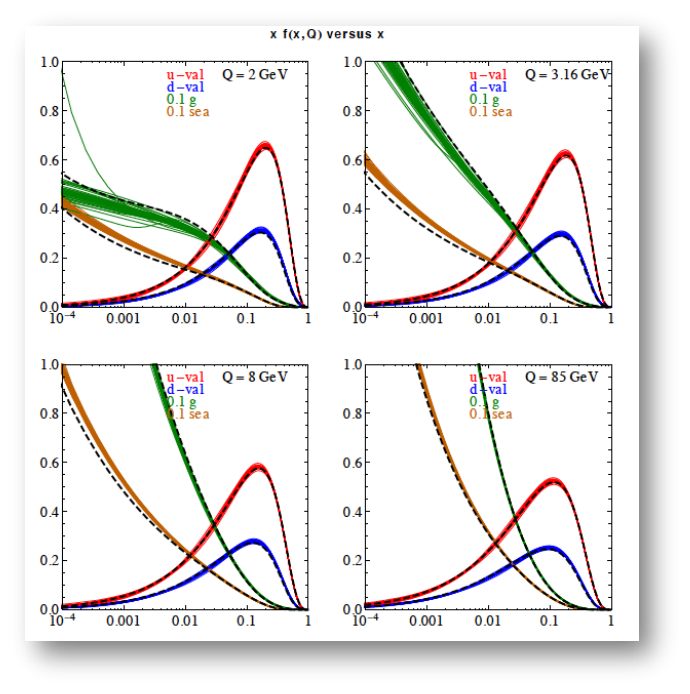
Exercise 5.5
Compute the anomalous dimension using Eq. (76).
6 Hadron collisions
While electron-positron annihilation and DIS played very important role in establishing pQCD for understanding high-energy scattering experiments, presently and in the mid-term future the experiments at the energy frontier can be found at the Large Hadron Collider (LHC). Thus we are most interested in the theoretical tools needed to understand high-energy proton-proton collisions.
6.1 Factorization theorem
Fortunately, the tools we have developed so far can be generalized straightforwardly to hadron collisions. The most general form of the factorization theorem includes convolution with two PDF’s, one for each colliding parton, the hard scattering cross section, and possibly a convolution with a fragmentation function (FF) of a parton into an identified hadron in the final state. Thus, the differential cross section for a hypothetical process has the form
| (81) |
In Eq. (81) is the total centre-of-mass energy squared, is the longitudinal momentum fraction of the pion in the parton , and are the renormalization and factorization scales, is the PDF for parton in the proton with momentum fraction , is the hard scattering cross section for the partonic process, is the FF for the process parton . The last term shows that contributions suppressed at high are neglected (). Substituting the PDF’s and FF’s with functions (in momentum and flavour) we obtain the cross section formulae in DIS and electron-positron annihilation.
The PDF’s and FF’s constitute the non-perturbative, long-distance components of the cross section that cannot be computed in pQCD, only extracted from measurements. Thus, it is a natural question whether or not the factorization theorem is predictive. The answer is a clear yes for the following reasons.
We can compute the hard scattering cross section in PT, which involves (i) renormalization of UV divergences (order by order in PT), (ii) cancellation of IR ones for IR safe observables using a subtraction method, (iii) absorbing initial state collinear divergences into renormalization of PDF’s (and possibly uncancelled final state ones into that of the FF). The non-perturbative components are universal, so can be measured in one process and used to make prediction in another one. Furthermore, the evolution of these with can be predicted in PT (DGLAP equations), shown in Fig. 18(b).
In summary, we are prepared to make predictions for any high-energy scattering process. The theoretical framework for such predictions relies on pQCD and the factorization theorem. In PT we can compute the hard scattering cross section and the evolution of the PDF’s. There are universal elements, such as the PDF’s and FF’s, as well as the subtraction method for computing radiative corrections.
6.2 Are we happy?
At this point theorists can make precision predictions for distributions of IR safe observables. The main bottleneck to make such predictions is the algebraic complexity of computing amplitudes and the analytic complexity of evaluating loop integrals. The state of the art considers the computation of NLO corrections a solved problem with automated implementations for processes up to about five partons in the final state (at tree level). The exact number depends on the process being considered because the numerical integrations become too expensive eventually. Nevertheless, all processes listed in the ‘Les Houches wishlist (2011)’ are known by now. Furthermore, there is also a computer code to compute seven-jet production in electron-positron annihilation [43].
For experimenters the situation is less satisfactory. While pQCD predictions are based on a solid theoretical ground, those lack important features. On the one hand pQCD gives predictions for final states with few partons, detectors detect hadrons. A tool that can simulate real events with hadrons at correct rates would be much more handy. To finish these lectures we look into modeling events in a qualitative way. A more detailed description can be found in Ref. [44].
6.3 Modelling events

Figure 19 shows our view of a proton-proton scattering event at high energy. The three parallel lines ending in discs from both sides represent the two incoming protons. At high energies these protons consist of (almost) free-flying partons, two of which (one from each) collide at high centre-of-mass energy and produce the hard scattering, with perturbatively computable cross section. This is where signs of new physics may appear. The hard scattering cross section is process dependent. We have discussed how it can be computed from first principles, which can be improved systematically by computing the radiative corrections.
Before collision the colliding partons may emit other partons collinear with the beam. These collinear emissions in the initial state give rise to divergences that can be factored into the renormalized parton distribution functions. After collision few energetic partons appear that may emit less energetic partons and each develops showers of partons. Emissions into almost the same direction as the original parton occur with enhanced probability (due to the collinear divergence) as well as emissions of soft gluon. This is represented in Figure 19 by red quark and gluon lines. Both factorization and parton showering can be described from first principles based upon known physics of QCD, and are universal, \ieindependent of the process and observable. We have seen how factorization works, but have not discussed how parton showers are modelled with shower Monte Carlo (SMC) programs [45, 46]. We mentioned marginally how the large logarithms emerging in the final state splittings can be resummed, which gives improved prediction for the cross section (as seen in Fig. 14), but does not simulate events.
Parton showers still only give a description of events in terms of quarks and gluons, whereas detectors detect only hadrons. We do not know how to compute hadronization, the transition from quarks and gluon to hadrons, from first principles. Yet the idea of local parton-hadron duality (LPHD) provides some sort of theoretical understanding (see, \egRef. [47]). It states that after accounting for all gluon and quark production down to scales , the transition from partons to hadrons is essentially local in phase space. Thus the hadron directions and momenta will be closely related to that of the partons, and the hadron multiplicity will reflect the parton multiplicity, too. This is illustrated by the green lines with dots.
In addition to the energetic partons in the initial state, there are also low-energy ones that may collide, which is energy and process dependent. This low-energy physics is described in models of underlying event, which are also part of modern SMC’s. The underlying event produces low-energy partons. Also at the end of the shower low-energy partons emerge. As QCD confines partons, these partons turn into hadrons before detection, a process called hadronization. We do not have a theory of hadronization based on first principles. Instead, SMC’s include models that describe hadronization in a process independent way. These models contain parameters that are fixed experimentally.
7 Conclusions
In these lectures we discussed the theoretical basis of interpreting the results of high-energy collider experiments. We discussed how pQCD can be made predictive and also the main uncertainties in the predictions. We used the following key ingredients in this tour: (i) gauge invariance that allows us to write down the Lagrangian and which predicts many important features of the theory; (ii) renormalization that cancels ultraviolet divergences systematically order-by-order in perturbation theory and introduces a dimensionful scale into even the scaleless Lagrangian of massless QCD, leading to scaling violations of one-scale observables that would be scale independent in the classical theory; (iii) asymptotic freedom at high energies emerging from the quantum structure of the theory and the non-Abelian nature of the gauge group; (iv) need for infrared safety, emerging from asymptotic freedom, to ensure that the IR divergences, associated with unresolved parton emission, cancel between real and virtual contributions, allowing the perturbative calculation of jet cross sections, without a detailed understanding of the mechanism by which partons become jets; (v) factorization that makes possible to use perturbative QCD to calculate the interactions of hadrons, since all the non-perturbative physics gets factorized, into parton distribution functions; (vi) evolution and universality of PDF’s that allows us to extract those measuring cross sections in one process, like DIS, and then used to predict the cross sections for any other process. Again, this factorization introduces a scale dependence into the parton model so that the structure functions of DIS, and other one-scale observables become scale dependent. These features make pQCD predictive, without forcing us to solve the theory at all possible scales: unknown or uncalculable high- and low-energy effects can be renormalized, factorized and cancelled away.
Acknowledgements
My lectures grew partly out of research conducted during the past 20 years and supported in part by Hungarian Scientific Research Fund grants, most recently under grant OTKA K-101482, and partly out of lectures given at Universities of Debrecen and Zürich where I received useful feedback from students. I benefited greatly from the lectures of previous schools by G. Salam [2] and F. Maltoni (http://physicschool.web.cern.ch/PhysicSchool/ESHEP/ESHEP2011/programme.html). I am grateful to the organizers, discussion leaders and students of the 2013 European School of High-Energy Physics for providing a pleasant and stimulating atmosphere.
References
- [1] H. Fritzsch, M. Gell-Mann, and H. Leutwyler, Advantages of the Color Octet Gluon Picture, Phys.Lett. B47 (1973) 365–368.
- [2] G. P. Salam, Perturbative QCD for the LHC, PoS ICHEP2010 (2010) 556, [arXiv:1103.1318].
- [3] Z. Nagy and Z. Trocsanyi, Four jet angular distributions and color charge measurements: Leading order versus next-to-leading order, Phys.Rev. D57 (1998) 5793–5802, [hep-ph/9712385].
- [4] OPAL Collaboration, G. Abbiendi et. al., A Simultaneous measurement of the QCD color factors and the strong coupling, Eur.Phys.J. C20 (2001) 601–615, [hep-ex/0101044].
- [5] J. Gasser and H. Leutwyler, Chiral Perturbation Theory to One Loop, Annals Phys. 158 (1984) 142.
- [6] J. Gasser and H. Leutwyler, Quark Masses, Phys.Rept. 87 (1982) 77–169.
- [7] J. Gasser and H. Leutwyler, Chiral Perturbation Theory: Expansions in the Mass of the Strange Quark, Nucl.Phys. B250 (1985) 465.
- [8] G. Colangelo, J. Gasser, and H. Leutwyler, scattering, Nucl.Phys. B603 (2001) 125–179, [hep-ph/0103088].
- [9] S. Durr, Z. Fodor, J. Frison, C. Hoelbling, R. Hoffmann, et. al., Ab-Initio Determination of Light Hadron Masses, Science 322 (2008) 1224–1227, [arXiv:0906.3599].
- [10] T. van Ritbergen, J. Vermaseren, and S. Larin, The Four loop beta function in quantum chromodynamics, Phys.Lett. B400 (1997) 379–384, [hep-ph/9701390].
- [11] L. Abbott, The Background Field Method Beyond One Loop, Nucl.Phys. B185 (1981) 189.
- [12] D. J. Gross and F. Wilczek, Ultraviolet Behavior of Nonabelian Gauge Theories, Phys.Rev.Lett. 30 (1973) 1343–1346.
- [13] H. D. Politzer, Reliable Perturbative Results for Strong Interactions?, Phys.Rev.Lett. 30 (1973) 1346–1349.
- [14] Particle Data Group Collaboration, J. Beringer et. al., Review of Particle Physics (RPP), Phys.Rev. D86 (2012) 010001.
- [15] M. Jamin and M. E. Lautenbacher, TRACER: Version 1.1: A Mathematica package for gamma algebra in arbitrary dimensions, Comput.Phys.Commun. 74 (1993) 265–288.
- [16] J. Alwall, M. Herquet, F. Maltoni, O. Mattelaer, and T. Stelzer, MadGraph 5 : Going Beyond, JHEP 1106 (2011) 128, [arXiv:1106.0522].
- [17] A. Pukhov, CalcHEP 2.3: MSSM, structure functions, event generation, batchs, and generation of matrix elements for other packages, hep-ph/0412191.
- [18] A. Pukhov, E. Boos, M. Dubinin, V. Edneral, V. Ilyin, et. al., CompHEP: A Package for evaluation of Feynman diagrams and integration over multiparticle phase space, hep-ph/9908288.
- [19] T. Hahn, Generating Feynman diagrams and amplitudes with FeynArts 3, Comput.Phys.Commun. 140 (2001) 418–431, [hep-ph/0012260].
- [20] ALEPH, DELPHI, L3, OPAL, SLD Collaborations, LEP Electroweak Working Group, SLD Electroweak Group, SLD Heavy Flavour Group, S. Schael et. al., Precision electroweak measurements on the resonance, Phys.Rept. 427 (2006) 257–454, [hep-ex/0509008].
- [21] K. Chetyrkin, Four-loop renormalization of QCD: Full set of renormalization constants and anomalous dimensions, Nucl.Phys. B710 (2005) 499–510, [hep-ph/0405193].
- [22] P. Baikov, K. Chetyrkin, J. Kuhn, and J. Rittinger, Complete QCD Corrections to Hadronic -Decays, Phys.Rev.Lett. 108 (2012) 222003, [arXiv:1201.5804].
- [23] Z. Bern, L. Dixon, F. Febres Cordero, S. Hoeche, H. Ita, et. al., Next-to-Leading Order -Jet Production at the LHC, Phys.Rev. D88 (2013) 014025, [arXiv:1304.1253].
- [24] G. Grunberg, Renormalization Group Improved Perturbative QCD, Phys.Lett. B95 (1980) 70.
- [25] P. M. Stevenson, Optimized Perturbation Theory, Phys.Rev. D23 (1981) 2916.
- [26] S. J. Brodsky, G. P. Lepage, and P. B. Mackenzie, On the Elimination of Scale Ambiguities in Perturbative Quantum Chromodynamics, Phys.Rev. D28 (1983) 228.
- [27] T. Kinoshita, Mass singularities of Feynman amplitudes, J.Math.Phys. 3 (1962) 650–677.
- [28] T. Lee and M. Nauenberg, Degenerate Systems and Mass Singularities, Phys.Rev. 133 (1964) B1549–B1562.
- [29] E. L. Berger, Research directions for the decade. Proceedings, 1990 Summer Study on High-Energy Physics, Snowmass, USA, June 25 - July 13, 1990, .
- [30] S. Catani, Y. L. Dokshitzer, M. Olsson, G. Turnock, and B. Webber, New clustering algorithm for multi - jet cross-sections in e+ e- annihilation, Phys.Lett. B269 (1991) 432–438.
- [31] ALEPH Collaboration, R. Barate et. al., Studies of quantum chromodynamics with the ALEPH detector, Phys.Rept. 294 (1998) 1–165.
- [32] Z. Nagy and Z. Trocsanyi, Multijet rates in e+ e- annihilation: Perturbation theory versus LEP data, Nucl.Phys.Proc.Suppl. 74 (1999) 44–48, [hep-ph/9808364].
- [33] M. Cacciari and G. P. Salam, Dispelling the myth for the jet-finder, Phys.Lett. B641 (2006) 57–61, [hep-ph/0512210].
- [34] M. Cacciari, G. P. Salam, and G. Soyez, The Anti-k(t) jet clustering algorithm, JHEP 0804 (2008) 063, [arXiv:0802.1189].
- [35] S. Catani, S. Dittmaier, M. H. Seymour, and Z. Trocsanyi, The Dipole formalism for next-to-leading order QCD calculations with massive partons, Nucl.Phys. B627 (2002) 189–265, [hep-ph/0201036].
- [36] JADE Collaboration, J. Schieck, S. Bethke, S. Kluth, C. Pahl, and Z. Trocsanyi, Measurement of the strong coupling from the three-jet rate in e+e- - annihilation using JADE data, Eur.Phys.J. C73 (2013) 2332, [arXiv:1205.3714].
- [37] G. Miller, E. D. Bloom, G. Buschhorn, D. Coward, H. DeStaebler, et. al., Inelastic electron-Proton Scattering at Large Momentum Transfers, Phys.Rev. D5 (1972) 528.
- [38] New Muon Collaboration, M. Arneodo et. al., Measurement of the proton and deuteron structure functions, F2(p) and F2(d), and of the ratio sigma-L / sigma-T, Nucl.Phys. B483 (1997) 3–43, [hep-ph/9610231].
- [39] J. Pumplin, D. Stump, J. Huston, H. Lai, P. M. Nadolsky, et. al., New generation of parton distributions with uncertainties from global QCD analysis, JHEP 0207 (2002) 012, [hep-ph/0201195].
- [40] Y. L. Dokshitzer, Calculation of the Structure Functions for Deep Inelastic Scattering and e+ e- Annihilation by Perturbation Theory in Quantum Chromodynamics., Sov.Phys.JETP 46 (1977) 641–653.
- [41] V. Gribov and L. Lipatov, Deep inelastic e p scattering in perturbation theory, Sov.J.Nucl.Phys. 15 (1972) 438–450.
- [42] G. Altarelli and G. Parisi, Asymptotic Freedom in Parton Language, Nucl.Phys. B126 (1977) 298.
- [43] S. Becker, D. Goetz, C. Reuschle, C. Schwan, and S. Weinzierl, NLO results for five, six and seven jets in electron-positron annihilation, Phys.Rev.Lett. 108 (2012) 032005, [arXiv:1111.1733].
- [44] P. Skands, Introduction to QCD, arXiv:1207.2389.
- [45] T. Sjostrand, S. Mrenna, and P. Z. Skands, PYTHIA 6.4 Physics and Manual, JHEP 0605 (2006) 026, [hep-ph/0603175].
- [46] G. Corcella, I. Knowles, G. Marchesini, S. Moretti, K. Odagiri, et. al., HERWIG 6: An Event generator for hadron emission reactions with interfering gluons (including supersymmetric processes), JHEP 0101 (2001) 010, [hep-ph/0011363].
- [47] Y. L. Dokshitzer, V. A. Khoze, A. H. Mueller, and S. I. Troyan, Basics of Perturbative QCD, Editions Frontieres, Gif-sur-Yvette, 1991.
- [48] R. Ellis, J. Stirling, and B. Webber, QCD and Collider Physics, Cambridge University Press, 1996.
- [49] G. G.Dissertori, I. Knowles, and M. Schmelling, High-Energy Experiments and Theory, Clarendon, Oxford, 2003.
- [50] CTEQ Collaboration, R. Brock et. al., Handbook of perturbative QCD: Version 1.0, Rev.Mod.Phys. 67 (1995) 157–248.