Light gauge boson in rare $K$ decay

A light gauge boson $X$ has been studied widely for various reasons [1, 2, 3, 4, 5, 6, 9, 7, 8, 10]. In particular, a mass of around 17 MeV boson with more than $5\sigma$ significance is indicated by the measurement of $e^{+}e^{-}$ angular correlations in the ${}^{8}Be$ transition [11], where the implications of this light gauge boson are investigated [12, 13, 14, 15].

However, two conclusions associated with the $X$ emission in rare $K$ decay appear in the literature, where some authors [16, 17] concluded that the longitudinal component in the $K^{-}\to\pi^{-}X$ decay is enhanced by $\epsilon_{X}\cdot p_{K}\sim m^{2}_{K}/m_{X}$, but others [4, 5, 18] showed that this decay amplitude should be suppressed by $\epsilon_{X}\cdot p_{K}m^{2}_{X}/m^{2}_{K}\sim m_{X}$.

In general, the decay amplitude for the $K^{-}\to\pi^{-}X$ process can be written as $A_{\lambda}=\langle X\pi^{-}|H_{I}|K^{-}\rangle=M_{\mu}\epsilon^{\mu}_{X}(k,\lambda)$, where $H_{I}$ is the involved interaction; $M_{\mu}$ is the transition matrix element for $K^{+}\to\pi^{+}$, and $\epsilon^{\mu}_{X}(\lambda)$ denotes the $X$ polarization vector with the momentum $k$ and helicity $\lambda$. Thus, the spin-average amplitude square can be expressed as:

If the charge, which is associated with gauge symmetry for the $X$-gauge boson, is conserved, following the current conservation $k^{\mu}M_{\mu}=0$, it can be seen that the term $k^{\mu}k^{\nu}/m^{2}_{X}$ vanishes. Clearly, the $1/m_{X}$ enhancement for a light gauge boson is associated with the charge nonconservation, i.e., $k^{\mu}M_{\mu}\neq 0$. Accordingly, the $1/m_{X}$ factor indeed is suppressed when the associated current is conserved, such as the case of a dark photon that mixes with the photon through the kinetic term [20, 21]. Furthermore, due to gauge invariance, the decay amplitude for $K^{+}\to\pi^{+}X$ in such cases should vanish at the tree level according to chiral perturbation theory [19]; the main contributions then are from the loop effects. A detailed analysis about the dark-photon case can be found in Refs. [4, 5].

To obtain a further understanding the properties of $K^{-}\to\pi^{-}X$ in the model with charge nonconservation, in this study, we analyze this issue by exploring the situations with and without the $SU(3)$ limit and unique gauge coupling when the $K^{-}\to\pi^{-}$ transition arises from the $W$-boson annihilation. In addition, we also study the contributions from the loop-induced flavor-changing neutral current (FCNC) process $s\to dX$.

Since our purpose is to investigate the properties of a light gauge boson emission from the $K^{-}\to\pi^{-}$ transition, we do not focus on a specific gauge model. Instead, we study a case in which the $X$-boson vectorially couples to the standard model (SM) quarks and the interactions are dictated by:

In general, the couplings $g_{qq^{\prime}}$ are flavor-dependent, and the FCNCs at the tree level are then induced. Since we have little knowledge on the flavor mixings, the associated FCNC parameters are completely free. We thus skip discussions on the tree-level FCNC effects in this work by assuming that they are small, or that they can always be constrained by low energy physics. In the following analysis, we focus on couplings with $q=q^{\prime}$ by writing $g_{q}\equiv g_{qq}$ for simplicity.

In order to demonstrate the characteristics of the $K^{-}\to\pi^{-}X$ decay, we analyze the hadronic effects with leading-twist parton distribution amplitudes (DAs) for the $\pi$ and $K$ mesons. As usual, the twist-2 DA of a pseudoscalar meson is defined by [22, 23]:

where $\xi=2u-1$, $\int^{1}_{0}du\,\phi_{P}(u)=1$, and $f_{P}$ is the decay constant of a meson $P$. The DA can be expanded by Gegenbauer polynomials as:

where the Gegenbauer moments $a^{P}_{i}$ for the $\pi$ and $K$ mesons at $\mu=1$ GeV are $a^{\pi}_{2i+1}=0$, $a^{\pi}_{2}=0.44$, $a^{\pi}_{4}=0.25$, $a^{K}_{1}=0.17$, and $a^{K}_{2}=0.2$ [22, 23, 24]. It can be seen that due to breaking of the $SU(3)$, the odd moments in the $K$ meson do not vanish. To calculate the $X$ emission from the $K$ and $\pi$ mesons, we adopt the spin structure for incoming meson as [25, 26]:

where $N_{c}=3$ is the number of colors, and the spin structure for outgoing meson can be obtained by using $\gamma_{5}\not{p}$ instead of $\not{p}\gamma_{5}$. According to Eq. (5), the $f_{P}$ can be obtained by taking the trace in spinor space as:

where the $N_{c}$ in the numerator is from the sum of color charges of quark line $\bar{q}_{2\alpha}[...]q_{1\alpha}$.

With the couplings in Eq. (2), the $K^{-}\to\pi^{-}X$ decay can arise from the tree and one-loop diagrams. Since the hadronic effects from the tree level are more copious than those from one-loop, we first discuss the tree contributions in detail. The flavor diagrams for the $K^{-}\to\pi^{-}X$ decay are shown in Fig. 1, where the square boxes and numbers denote the possible places to emit the $X$-boson. According to Eq. (5), the decay amplitude for the $X$-boson emitting from place-1 can be derived as:

It is found that the decay amplitude for the $X$-boson emitting from place-$j$ can be formulated as:

where $C_{K\pi}=G_{F}/(2\sqrt{2})V^{*}_{ud}V_{us}f_{K}f_{\pi}$, $g_{1,3}=g_{u}$, $g_{2}=g_{s}$, $g_{4}=g_{d}$, $\phi_{1,2}=\phi_{K}$, $\phi_{3,4}=\phi_{\pi}$, and $R_{j}$ are defined as:

In order to understand the $SU(3)$ limit and $g_{q}$ dependence of $A_{j}$, we study the cases by requiring an exact/partial $SU(3)$ limit and different/same $g_{q}$.

(I) SU(3) limit: $m_{K}=m_{\pi}\equiv m_{P}$, $\phi_{K}=\phi_{p}\equiv\phi_{P}$:
Since $f_{K}$ and $f_{\pi}$ are the multiplier factors, they are irrelevant to the discussions of the $SU(3)$ limit; therefore, we do not need to set $f_{K}=f_{\pi}$. Due to the kinematics, $p_{K}=p_{\pi}+p_{X}$ has to be satisfied; thus, we need to leave the factors $p_{X}\cdot p_{K}$ and $p_{X}\cdot p_{\pi}$, which appear in the denominators of Eq. (9), alone. From Eqs. (8) and (9), we then get:

and $A_{2}+A_{4}=-(g_{d}+g_{s})/(2g_{u})(A_{1}+A_{3})$. We consider $A_{1}+A_{3}$ because $A_{1}$ and $A_{3}$ involve the same gauge coupling $g_{u}$. One can alternatively use $A_{1}+A_{2}(A_{3}+A_{4})$ according to the convenience. It is clearly seen that the decay amplitude for the $K^{-}\to\pi^{-}X$ is proportional to $m^{2}_{X}$. This result matches the conclusions given in two earlier works [4, 18]. We note that when calculating $A_{2}+A_{4}$, we have used the property $\phi_{P}(x)=\phi_{P}(1-x)$, where this condition is suitable for the $\pi$ meson, and it is violated in the $K$ meson due to the breaking of $SU(3)$. As a result, the leading-twist contributions can not lead to an interesting result in the $SU(3)$ limit. Furthermore, if we further set $g_{s}+g_{d}=2g_{u}$, it can be found that $\sum A_{i}=0$.

(II) Partial SU(3) limit: $\phi_{K}=\phi_{\pi}\equiv\phi_{P}$
When we release the condition $m_{K}=m_{\pi}$, the first term in the numerator of Eq. (10) inside the integral becomes $m^{2}_{X}(m^{2}_{K}+m^{2}_{\pi})(1-x)-(m^{2}_{K}-m^{2}_{\pi})^{2}x$, and the denominator is $m^{4}_{X}(1-x)^{2}-(m^{2}_{K}-m^{2}_{\pi})^{2}x^{2}$. With $m_{X}=0$, we find:

where the $x$ dependence of the numerator and denominator in the integral is cancelled, and $\int^{1}_{0}\phi_{P}(x)dx=1$ is applied. By this analysis, it is clear that when we put back the $SU(3)$ breaking effect with $m_{K}\neq m_{\pi}$, the decay amplitude is not proportional to $m^{2}_{X}$ anymore. This result confirms the conclusions given in two earlier studies [16, 17]. Furthermore, if we take all gauge couplings to be the same and $m^{2}_{X}\neq 0$, we find that $\sum_{i}A_{i}=0$ is still satisfied. We can understand the cancellations from another viewpoint: by using $\phi_{P}(x)=\phi_{P}(1-x)$, from Eqs. (8) and (9) it can be easily found that $A_{1}+A_{2}=0$ for $g_{u}=g_{s}$ and $A_{3}+A_{4}=0$ for $g_{u}=g_{d}$.

(III) $SU(3)$ breaking
With a partial $SU(3)$ limit, which is conditioned by $\phi_{K}=\phi_{\pi}$, it can be seen that the decay amplitude for the $K^{-}\to\pi^{-}X$ is not suppressed by $m^{2}_{X}$; however, it diminishes when $g_{s}\sim g_{d}\sim g_{u}$. It is intriguing to see whether the cancellations work or not when the $SU(3)$ breaking effects are taken into account in the DA of the $K$ meson. From Eqs. (8) and (9), we can easily get the result $A_{4}=-g_{d}/g_{u}A_{3}$ when the $g_{u}$ and $x$ in $A_{3}$ are replaced by the $g_{d}$ and $1-x$. The connection between $A_{3}$ and $A_{4}$ is based on the property $\phi_{\pi}(x)=\phi_{\pi}(1-x)$, where the odd Gegenbauer moments vanish. That is, if $g_{d}=g_{u}$, the cancellation between $A_{3}$ and $A_{4}$ still works. Unlike the DA of pion, $\phi_{K}(x)\neq\phi_{K}(1-x)$ due to nonvanishing odd Gegenbauer moments, e.g., $a^{K}_{1}=0.17$. Hence, we have:

In order to examine Eq. (12), we simplify the analysis by taking the limit $m_{X}\to 0$. Thus, with $g_{s}=g_{u}$, we find:

According to the result, it can be seen that the decay amplitude for the $K^{-}\to\pi^{-}X$ with $g_{u}=g_{s}=g_{d}$ is $\sum_{i}A_{i}\propto a^{K}_{1}f(m^{2}_{X})$, where the function $f(m^{2}_{X})$ is from the integration in $x$ and only depends on the $m^{2}_{X}$. We then conclude that if the $X$ gauge couplings to the quarks are the same, the decay amplitude of the $K^{-}\to\pi^{-}X$ process from the leading-twist DA is suppressed by $m_{X}$. To illustrate the relative magnitude under the $SU(3)$ assumptions, we show the numerical values with some chosen values of couplings and $m_{X}$ in Table 1, where the function $M_{m_{X}}$ is defined as:

$SU(3)_{I,II,III}$ denote the cases for the $SU(3)$ limit, the partial $SU(3)$ limit, and the breaking of $SU(3)$.

It is of interest to examine the $X$ emission from the $W$-boson propagator shown in Fig. 1. To estimate the contribution, we parametrize the Lorentz covariant gauge coupling $WWX$ to be:

where $g_{WWX}$ is the trilinear gauge coupling; $p_{-}$, $p_{+}$, and $p_{X}$ are the momenta of the $W^{-}$, $W^{+}$, and $X$ gauge bosons, respectively, and the momenta are chosen to flow into the vertex. Accordingly, the decay amplitude for the $K^{-}\to\pi^{-}X$ via the trilinear coupling can be obtained as:

It is clear that the contribution from the coupling $WWX$ is suppressed by $m_{X}$. This result is nothing to do with the $SU(3)$ limit.

Without the $SU(3)$ limit, it can be seen from Eq. (9) that the numerators of $R_{1,2}$ are related to $m^{2}_{\pi}$ and that those of $R_{3,4}$ are associated with $m^{2}_{K}$. Since $m_{K}$ is around 3.5 times larger than $m_{\pi}$, numerically, the values of $A_{1,2}$ are one order of magnitude smaller than those of $A_{3,4}$. As a result, the $BR(K^{-}\to\pi^{-}X)$ is sensitive to the difference between $g_{d}$ and $g_{u}$. To present the numerical analysis, we adopt $g_{u}$ and $g_{d}-g_{u}$ as the free parameters and set $g_{s}=g_{d}$. We show the contours for $BR(K^{-}\to\pi^{-}X)$ (in units of $10^{-7}$) as a function of $g_{u}$ and $g_{d}-g_{u}$ (in units of $10^{-3}$) in Fig. 2, where we have used $f_{K}=0.16$ GeV and $f_{\pi}=0.13$ GeV, and the numbers on the lines denote the values of $BR(K^{-}\to\pi^{-}X)$. With the assumption of $BR(X\to e^{+}e^{-})\sim 1$, we obtain $BR(K^{-}\to\pi^{-}e^{+}e^{-})\approx BR(K^{-}\to\pi^{-}X)$, where the current measurement is $BR^{\rm exp}(K^{-}\to\pi^{-}e^{+}e^{-})=(3.00\pm 0.09)\times 10^{-7}$ [28]. Therefore, the dashed lines in the plot can be regarded as the central value of the experimental measurement. From the figure it can be seen that $|g_{d}-g_{u}|$ cannot be larger than $10^{-4}$.

In addition to the tree-level $W$-boson annihilation, the FCNC coupling $sdX$, which is induced from one-loop and is depicted in Fig. 3, can also contribute to the $K^{-}\to\pi^{-}X$ process. According to the interactions in Eq. (2), the effective coupling of $sdX$ from each up-type quark loop can be derived as:

where we have dropped the small effects from $m_{s,d}$; the factor $m^{2}_{q}$ is from the mass inserted twice in $q$-quark propagator, and $I_{q}(r)$ is the loop integral. From Eq. (17), the associated Cabibbo-Kobayashi-Maskawa (CKM) matrix elements for top-quark loop are $V^{*}_{td}V_{ts}$, and due to the enhancement of $m^{2}_{t}$, its contribution is comparable to that from the charm-quark, in which the essential factor is $m^{2}_{c}V^{*}_{cd}V_{cs}$. The contribution from the $u$-quark loop can be ignored because of the $m^{2}_{u}$ suppression. Additionally, it can be clearly seen that although the $X$ couplings to quarks are vector-like, the induced coupling $sdX$ indeed is chiral.

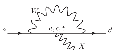
Unlike the $W$-boson annihilation shown in Fig. 1, the dominant hadronic effect for the $K^{-}\to\pi^{-}X$ decay from $sdX$ interaction is formulated by [27]:

where $f_{+}\approx 0.971$ at $q^{2}=0$. As a result, the corresponding transition amplitude and BR are respectively given by:

It can be seen that Eq. (19) is not suppressed by $m_{X}$ but rather is enhanced by $1/m_{X}$. This result is consistent with the dark $Z$ model in Ref. [5] if we set $g_{q}\sim\delta\,m_{X}/m_{Z}$. To show the bounds on the gauge couplings $g_{t}$ and $g_{c}$ independently, we present the numerical values of Eq. (19) as a function of $g_{t}$ and $g_{c}$ in Fig. 4, where $m_{X}=17$ MeV is used, the solid (dashed) line stands for the result of $g_{t}(g_{c})$ in units of $10^{-5}$, and the horizontal dotted line is the central value of $BR^{\rm exp}(K^{-}\to\pi^{-}e^{+}e^{-})$. With $BR(X\to e^{+}e^{-})\sim 1$, the bounds from the penguin diagrams are stronger than those from the $W$-boson annihilations. Therefore, we confirm the conclusion given in a previous work [17], where the effective coupling arising from the penguin diagrams obtains a stricter bound. We note that the $X$-boson emitting from the $W$ propagator shown in Fig. 3 can also contribute to $K^{-}\to\pi^{-}X$; however, due to the $m^{2}_{K}/m^{2}_{W}$ suppression, we neglect its contribution in the numerical analysis.

In summary, a light gauge boson predominantly decaying to $e^{+}e^{-}$ in rare $K$ decay is studied. The process $K^{-}\to\pi^{-}X\to\pi^{-}e^{+}e^{-}$ can be generated from both tree and penguin diagrams. It is found that the decay amplitude for $K^{-}\to\pi^{-}X$ from $W$-boson annihilation can be directly proportional to $m^{2}_{X}\epsilon_{X}\cdot p_{K}$ when the $SU(3)$ limit is applied, or when the gauge couplings satisfy $g_{u}=g_{d}=g_{s}$. When these conditions are relaxed, it is found that if $g_{u}$ is of the ${\cal O}(10^{-3})$, $|g_{d}-g_{u}|$ has to be less than $10^{-4}$. By contrast, the $m^{2}_{X}$ suppression is not found in the loop-induced $K^{-}\to\pi^{-}X$ process. We show that the loop effects indeed produce more severe bounds on the gauge couplings $g_{t}$ and $g_{c}$. Our results are consistent with the conclusions given in two previous studies [16, 17].

References

- [1] S. N. Gninenko and N. V. Krasnikov, Phys. Lett. B 513, 119 (2001) [hep-ph/0102222].
- [2] P. Fayet, Phys. Rev. D 75, 115017 (2007) [hep-ph/0702176 [HEP-PH]].
- [3] N. Arkani-Hamed, D. P. Finkbeiner, T. R. Slatyer and N. Weiner, Phys. Rev. D 79, 015014 (2009) [arXiv:0810.0713 [hep-ph]].
- [4] M. Pospelov, Phys. Rev. D 80, 095002 (2009) [arXiv:0811.1030 [hep-ph]].
- [5] H. Davoudiasl, H. S. Lee and W. J. Marciano, Phys. Rev. D 89, no. 9, 095006 (2014) [arXiv:1402.3620 [hep-ph]].
- [6] K. Petraki, L. Pearce and A. Kusenko, JCAP 1407, 039 (2014) [arXiv:1403.1077 [hep-ph]].
- [7] T. Araki, F. Kaneko, T. Ota, J. Sato and T. Shimomura, Phys. Rev. D 93 (2016) no.1, 013014 [arXiv:1508.07471 [hep-ph]].
- [8] S. Baek, Phys. Lett. B 756, 1 (2016) [arXiv:1510.02168 [hep-ph]].
- [9] H. S. Lee and S. Yun, Phys. Rev. D 93, no. 11, 115028 (2016) [arXiv:1604.01213 [hep-ph]].
- [10] P. Ko and Y. Tang, arXiv:1608.01083 [hep-ph].
- [11] A. J. Krasznahorkay et al., Phys. Rev. Lett. 116, no. 4, 042501 (2016) [arXiv:1504.01527 [nucl-ex]].
- [12] J. L. Feng, B. Fornal, I. Galon, S. Gardner, J. Smolinsky, T. M. P. Tait and P. Tanedo, arXiv:1604.07411 [hep-ph].
- [13] P. H. Gu and X. G. He, arXiv:1606.05171 [hep-ph].
- [14] L. B. Chen, Y. Liang and C. F. Qiao, arXiv:1607.03970 [hep-ph].
- [15] Y. Liang, L. B. Chen and C. F. Qiao, arXiv:1607.08309 [hep-ph].
- [16] P. Fayet, Nucl. Phys. B 187, 184 (1981).
- [17] M. Suzuki, Phys. Rev. Lett. 56, 1339 (1986).
- [18] T. M. Aliev, M. I. Dobroliubov and A. Y. Ignatiev, Phys. Lett. B 221, 77 (1989).
- [19] G. Ecker, A. Pich and E. de Rafael, Nucl. Phys. B 291, 692 (1987).
- [20] B. Holdom, Phys. Lett. B 166, 196 (1986).
- [21] J. Jaeckel, M. Jankowiak and M. Spannowsky, Phys. Dark Univ. 2, 111 (2013) [arXiv:1212.3620 [hep-ph]].
- [22] V. M. Braun and I. E. Filyanov, Z. Phys. C 48, 239 (1990) [Sov. J. Nucl. Phys. 52, 126 (1990)] [Yad. Fiz. 52, 199 (1990)].
- [23] P. Ball, JHEP 9901, 010 (1999) [hep-ph/9812375].
- [24] P. Ball, JHEP 9809, 005 (1998) doi:10.1088/1126-6708/1998/09/005 [hep-ph/9802394].
- [25] C. H. Chen, Y. Y. Keum and H. n. Li, Phys. Rev. D 64, 112002 (2001) [hep-ph/0107165].
- [26] C. H. Chen and H. Hatanaka, Phys. Rev. D 73, 075003 (2006) [hep-ph/0602140].
- [27] N. Carrasco, P. Lami, V. Lubicz, L. Riggio, S. Simula and C. Tarantino, Phys. Rev. D 93, no. 11, 114512 (2016) [arXiv:1602.04113 [hep-lat]].
- [28] K.A. Olive et al. (Particle Data Group), Chin. Phys. C, 38, 090001 (2014).