Managing resonant trapped orbits in our Galaxy
Abstract
Galaxy modelling is greatly simplified by assuming the existence of a global system of angle-action coordinates. Unfortunately, global angle-action coordinates do not exist because some orbits become trapped by resonances, especially where the radial and vertical frequencies coincide. We show that in a realistic Galactic potential such trapping occurs only on thick-disc and halo orbits (speed relative to the guiding centre ). We explain how the Torus Mapper code (TM) behaves in regions of phase space in which orbits are resonantly trapped, and we extend TM so trapped orbits can be manipulated as easily as untrapped ones. The impact that the resonance has on the structure of velocity space depends on the weights assigned to trapped orbits. The impact is everywhere small if each trapped orbit is assigned the phase space density equal to the time average along the orbit of the DF for untrapped orbits. The impact could be significant with a different assignment of weights to trapped orbits.
Keywords:
Galaxy: kinematics and dynamics – galaxies: kinematics and dynamics – methods: numerical1 Introduction
The volume and quality of the data we have to characterise both our own Galaxy and many external galaxies has increased enormously over the last decade, and continues to increase rapidly through technological advances such as ESA’s astrometric satellite Gaia and a new generation of integral-field units such as ESO’s instrument MUSE. Adequate exploitation of the superb data now accumulating must involve the construction of intricate chemodynamical models of galaxies that include fully dynamical dark matter and several populations of stars of varying age and chemical composition.
A promising approach to the construction of such models involves specifying the distribution functions (df) of several populations as analytic functions of action integrals, and then determining the gravitational potential that these populations jointly generate. Once that has been done, a prediction for essentially any observable quantity can be extracted from the model, and the model can be fitted to one or more data sets by adjusting the parameters in the dfs.
Over the last several years we have been pursuing this line of attack in the context of modelling our Galaxy (Binney, 2010; Binney & McMillan, 2011; Sanders & Binney, 2013; Piffl et al., 2014; Sanders & Binney, 2015; Binney & Piffl, 2015). This approach has been fruitful. For example, it revealed that the Local Standard of Rest deduced from Hipparcos data and used for over a decade was in error (Binney, 2010). It has also provided by far the tightest constraints on the mass of dark matter interior to the solar radius (Piffl et al., 2014) and demonstrated for the first time that at Galactocentric radii baryons have materially modified the phase-space density of dark matter (Binney & Piffl, 2015). Schönrich & McMillan (2016) have used models in which a large number of chemically distinct stellar populations each has a df to explain the connection between inside-out growth of our Galaxy and correlations between rotation velocity and chemistry.
The work just described rests on the assumption that realistic galactic potentials admit global angle-action variables. Unfortunately, global angle-action variables only exist when a resonant condition between the fundamental frequencies of an orbit never leads to the orbit becoming trapped by the resonance. In typical galactic potentials some orbits do become resonantly trapped, so these potentials do not admit global angle-action coordinates. Given this inconvenient truth, could an approach to galaxy modelling that predicates the existence of global angle-action coordinates be misleading? Can angle-action variables be extended to cover resonantly trapped orbits? The purpose of this paper is to address these questions.
A cornerstone of our work is provided by the Torus Mapper (tm), a numerical code that fits null tori to a given Hamiltonian (Binney & McMillan, 2016).11 1 This code can be downloaded from github.com/PaulMcMillan-Astro/Torus. Using tm one can construct a Hamiltonian that closely approximates the given Hamiltonian and admits global angle-action coordinates. The procedure is as follows (Kaasalainen & Binney, 1994; Binney & McMillan, 2016). At each point on a grid in action space, tm is used to construct a torus, that is functions and that give the ordinary phase-space coordinates in terms of the angle variables `. From these tori a torus can be constructed for any point in action space by interpolation. The Hamiltonian is then defined to be the angle average of the given Hamiltonian over this torus. Clearly the resulting tori are, by construction, the orbital tori of and define a global system of angle-action coordinates. Once and its angle-action coordinates have been constructed, perturbation theory can be used to study resonant trapping of orbits in , but in the Galaxy modelling work cited above we have simply ignored resonant trapping. In some sense ignoring resonant trapping is equivalent to approximating our Galaxy’s Hamiltonian by the integrable Hamiltonian .
In this paper we show how to proceed to the next level of approximation, in which we recognise zones of missing actions in the basic action space, and with each such zone associate a family of resonantly trapped orbits.
In Section 2 we introduce the model Galaxy potential that is used throughout and recall the principles of surfaces of section. In Section 3 we explain why at any energy of interest the resonance will occur, and determine the critical value of the peculiar velocity that a star with the angular momentum of the Sun must have in order to become resonantly trapped. In Section 4 we show how tm behaves when asked to produce a torus that has, in fact, become trapped. In Section 5 we use Hamiltonian perturbation theory to construct tori for trapped orbits. In Section 6 we use tm to construct different kinds of resonantly trapped orbits in a realistic Galactic potential, and investigate the extent of resonant trapping in this potential. We investigate the seriousness of the errors made by ignoring the existence of resonant trapping, and explain how tm can be used to determine the density of stars in velocity space when resonant trapping is taking into account. Finally, in Section 7 we sum up and look to the future. An appendix explains in more detail why tm makes a sudden transition at the centre of a zone of missing actions.
2 The Galactic potential
We frame our discussion in the context of a gravitational potential that McMillan (2011) fitted to a variety of data for our Galaxy. Specifically, we adopt the “best” potential in that paper, which is generated by thin and thick stellar discs, a flattened (axisymmetric) bulge and a spherically symmetric dark halo. Its local circular speed is . Our discussion would not differ materially, however, had we adopted any reasonably realistic axisymmetric potential. To evaluate the potential and its derivatives we use the falPot code distributed in the tm package, which implements an algorithm described by Dehnen & Binney (1998), and was extracted from Walter Dehnen’s falcON package.

Motion in an axisymmetric potential can be reduced to motion in the plane under the Hamiltonian
| (1) |
where
| (2) |
That is, we study motion with just two degrees of freedom under a Hamiltonian that contains the angular momentum as a parameter. Deep insight into such motion is provided by surfaces of section (sos) in which we plot a point in the plane every time the particle crosses the equatorial plane moving upwards. All such “consequents” correspond to phase-space point at a given energy at which , so these points are subject to two constraints on the four phase-space coordinates. If the orbit admits a third integral, , this third constraint on the phase-space coordinates restricts the consequents to one degree of freedom, and they lie on a curve. Fig. 1 shows a surface of section for roughly the angular momentum of the Sun. The points in this sos clearly lie along a series of curves, so an integral is respected by these orbits. Each curve contains the consequents of a single orbit.
The curves in Fig. 1 form a bull’s eye. At the centre would lie the single point of the shell orbit , which is the generalisation to a flattened potential of a circular orbit that is inclined to the equatorial plane. The curve of black points that runs around the edge, is formed by the eccentric, planar orbit . Hence, as one proceeds from the middle to the edge, successive curves are generated by orbits of increasing eccentricity and decreasing inclination.
3 The 1:1 resonance near the Sun

A resonance occurs whenever the fundamental frequencies of a quasi-periodic orbit satisfy a relationship , where is a vector with integer components. The dynamical impact of a resonance rapidly decreases with the modulus , so by far the most important resonance for studies of our Galaxy is the resonance at which . In our adopted potential, the disc being massive and thin causes the radial epicycle frequency of circular orbits to be smaller than the vertical epicycle frequency for . Consequently, for disc orbits of low inclination, . By contrast, on the highly inclined orbits of most halo stars because for a spherical system with a flat circular-speed curve, and . Hence given sufficient energy of motion in the plane, somewhere along a sequence of orbits of decreasing and increasing , one will encounter the resonant condition .
To encounter the 1:1 resonance one has to consider more energetic orbits than those plotted in Fig. 1, which all have . In the present potential, orbits with the angular momentum of the Sun can become resonantly trapped only if they have sufficient energy to pass the Sun at a speed in excess of .
Whereas the orbits in the sos of Fig. 1 were obtained by launching particles from with a speed in the plane of , the orbits in Fig. 2 were obtained by launching particles with speed . Now there are orbits, with consequents plotted in blue, that are trapped by the 1:1 resonance. The innermost (black) curves are generated by orbits with , while the black curves that lie beyond the blue curves are generated by orbits on which . Between these regimes lie orbits of intermediate eccentricity on which is so small that they become trapped. The orbits generating the blue points always pass upwards through the plane at small radii and downwards at large radii, so they circulate clockwise in the plane. Other orbits, for which no consequents are plotted, circulate in the opposite sense and would occupy the vacant region around – we will discuss these oppositely circulating orbits in Section 6 below.
4 TM at resonances


Fig. 3 shows two examples of how tm generates tori at the energy and angular momentum of Fig. 2. Each panel is constructed by finding for the shell orbit that has the correct energy, and then incrementing in steps while decrementing in steps in order to keep the energy constant. For each pair of actions a torus is found and used to draw a red curve. The only difference in the procedure used to plot each panel of Fig. 3 is that in the upper panel we specified tolerance , whereas for the lower panel we specified .
The torus that wraps around the left side of the island of blue, trapped orbits in Fig. 2 has , while the torus that touches the right edge of the island has . Hence for the studied energy, there are no orbits with in the range ; this is a zone of “missing actions” (ZoMA) in the notation of Binney & Spergel (1984).
The pattern of red curves in the upper panel of Fig. 3 is unsatisfactory in that a few red curves cross other red curves. If each red curve really were a cross section through a torus of the specified energy, from a point of intersection one could complete the phase-space coordinates by deducing from the energy, and on integrating the orbit the consequents could lie on at most one of the red curves. Hence red curves can intersect only if the Hamiltonian does not take the same, constant, value on both the generating tori. Hence in Fig. 3 an intersection of red curves implies that at least one of the responsible tori is not an orbital torus.
When the actions specified are those of a trapped orbit, tm cannot fit a torus with the given actions exactly into the phase-space hypersurface because no such torus exists. Given a sufficiently large value of the tolerance parameter , it returns a torus that is smooth but fluctuates in energy. Given a smaller value of , it reduces the fluctuations in energy just a little by returning a torus that depends sensitively on the input actions.
We usually want the tori returned by tm to be extensible to the basis of an integrable Hamiltonian. Intersecting tori do not form such a basis, so they should be avoided. The lower panel of Fig. 3 shows that in this instance we can obtain tori that form a basis for the construction of an integrable Hamiltonian simply by increasing the tolerance parameter to .

A different strategy for avoiding intersecting tori is to use a small value of but to reject tori returned by tm with a non-zero value of the variable flag, indicating that the requested rms variation of the Hamiltonian over the constructed torus was not achieved. Fig. 4 illustrates this possibility. Now we have a consistent set of fits to all un-trapped tori, and a clean gap left in the trapping region.
4.1 Coefficients returned by TM

In this section we ask how tm responds when asked to compute a torus that has actually become trapped so it is impossible to drive the mean-square value of the residual Hamiltonian
| (3) |
with , below some smallest, non-zero value.
tm generates tori as images of the analytic torus of the isochrone Hamiltonian under a canonical map. Normally the generating function of this map is (Binney & McMillan, 2016)
| (4) |
where denotes the angle variables of the isochrone Hamiltonian and is a two-vector with integer components. tm minimises with respect to the parameters of the isochrone Hamiltonian and the coefficients in equation (4) – below we consider the set of all the quantities to be adjusted to form the components of the vector . The analytic Hamiltonian (in this case the isochrone Hamiltonian) is referred to as the “toy” Hamiltonian, and the superscript T on ` in equation (4) indicates that the components of ` are the angle variables of the toy Hamiltonian.
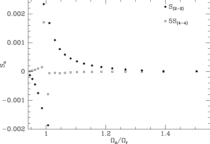
When tori are computed for a progression of actions that includes resonantly trapped tori, one expects the magnitudes of coefficients for which to be large on either side of the resonance, reflecting a growing need to distort the toy torus into the true torus. Moreover, surfaces of section such as Fig. 4 suggest that these resonant coefficients will have opposite signs on each side of the resonance, because the toy tori are clearly stretched in opposite senses (horizontally/vertically) on each side of the resonance. So we expect the resonant to become large and positive as we approach the resonance from one direction, to change sign in the ZoMA, and then to diminish from a large negative value as we recede from the resonance. The upper panel of Fig. 5 confirms this prediction by plotting against frequency ratio the values of and along the sequence of tori that make up the surface of section Fig. 4. The lower panel of Fig. 5, which has a logarithmic axes, shows how strongly the importance of the resonant coefficients grows as one approaches by plotting sums of over resonant and non-resonant values of .
4.2 When do tori cross?

If we want to use tori returned by tm to define an integrable Hamiltonian, it is vital that neighbouring tori do not cross in any surface of section. From the generating function (4) we have that
| (5) |
Two tori, and will cross if a single phase-space point can be reached from both tori. The tori most likely to cross are those on either side of the resonance because, as we have seen, then . Since is unity somewhere on the tori and often changes sign across a resonance, crossing is likely if
| (6) |
where the sum is over resonant . In Fig. 6 the nearly horizontal lines show the differences in and between adjacent tori in the upper sos of Fig. 3 and the dots show twice the value of the sum
| (7) |
which changes sign across the resonance. The region in which the dots lie above the horizontal lines, implying the likelihood of tori crossing, coincides quite well with the ZoMA, the boundaries of which are marked by the vertical lines. Evidently, if the tori are required to form an integrable Hamiltonian, the sum (7) should be prevented from exceeding .
5 Perturbation theory
When on some torus the resonance condition is satisfied, one should use perturbation theory to investigate the possibility of resonant trapping. In the vicinity of the resonance, the angle variable
| (8) |
will evolve slowly and we make a canonical transformation to new angle-action variables that include this variable. A suitable generating function is
| (9) |
Indeed, then from one recovers equation (8) and . From we find
| (10) | ||||||
| (11) | ||||||
| (12) |
It is worth noting that
| (13) |
so when we vary while holding fixed, we are considering orbits of a common energy, as in a surface of section.
We Fourier expand the Hamiltonian in the new angle variables
| (14) |
where because the are close to the actions of . The new actions have the equations of motion
| (15) |
We average these equations over and on the grounds that these variables move through a complete cycle in times that are much shorter than the smallest time . Since the equations of motion for only contain terms with non-trivial dependence on , the right sides of these equations vanish after averaging, and we conclude that are effective constants of motion: on short timescales they wiggle slightly, but on long timescales they do not change. From equations (10) we see that the constancy of implies that when , any variation in will be reflected in a complementary variation in .
The averaged equations of motion can be derived from the Hamiltonian obtained by averaging equation (14) over :
| (16) |
where and we have omitted references to the constant actions . Since this a time-independent Hamiltonian, the motion occurs on the curve in the plane on which , a constant. A good approximation to this motion can be obtained by Taylor expanding the functions of in equation (16). However, before we do so we exploit the reality of to write
| (17) |
where the are the phases of the . We expand and to second order in
| (18) |
where is the primed action of the resonant torus. Since a constant term in can be discarded and we know that on the resonant torus (eq. 13), we replace by , where
| (19) |
The Taylor series for ,
| (20) |
cannot be simplified in this way, so the equation becomes
| (21) | ||||
| (22) | ||||
| (23) |
In this approximation we can determine simply by solving the quadratic equation (21) for given . Given the fluctuating value of and the constants , we can recover the complete action-space coordinates from equations (10). In general all three components of oscillate but in such a way that is to leading order constant.
If we retain only one value of and neglect and , equation (21) reduces to the energy equation of a pendulum, and this is traditionally used to discuss resonant trapping (Chirikov, 1979, e.g.). Kaasalainen (1994) demonstrated the merit retaining and . In the application to the Galaxy good results can be obtained with just the dominant value of , but perceptibly better results are obtained at trifling extra cost by retaining two values of , so that is what we do.
5.1 Action and angle of libration
The range through which oscillates is set by the condition that the quadratic for has real roots:
| (24) | ||||
| (25) |
In our application to the Galaxy below we have . This being so, and bearing in mind that the are by definition all non-negative, oscillates around for the dominant value of . The largest permitted value of is set by adopting the equals sign in equation (24) with for the dominant value of , and similarly for the smallest permitted value of .
Rather counter-intuitively, , the smallest value of , corresponds to the orbit that has the largest-amplitude librations around the resonant orbit. The reason does not function like a conventional energy is that , which in equation (21) plays the role of mass, is negative.
Each value of corresponds to an action that quantifies the extent to which a trapped orbit oscillates around the trapping torus. is straightforwardly computed as
| (26) |
where the dependence of on is obtained from equation (21). Since increases from its minimum to its maximum value with given by the larger root of the quadratic (21) and returns to its minimum value with given by the smaller root, is give by the difference of the roots integrated over the range of .
On a trapped orbit, is not an angle variable, although are angle variables. Since the missing angle variable evolves linearly in time, it is
| (27) |
where from Hamilton’s equation and equation (17) we have
| (28) |
In this equation is by the quadratic equation (21) a function of .
| resTorus(Tgr,Jrgr,n,Jb,G,hn) | Tgr and Jrgr pointers to array of n untrapped tori and their radial actions. Jb actions of underlying resonant torus, G derivative of , hn pointer to , and their derivatives on torus Jb. |
|---|---|
| I,Imin,Imax | The value of on this torus and the smallest and largest permitted values of . |
| setI(I) | Sets value of |
| librationAction() | Returns action of libration. |
| librationOmega() | Returns frequency of libration. |
| FullMap(A) | Returns at given angles. |
| SOS(ofile,n) | Places in ofile n consequents in SoS. |
| SOSr(ofile,n) | As SOS but for the orbit rotating counterclockwise in the plane. |
| containsPoint_Ang(Rzphi,A,t1) | Returns number of times torus passes through point Rzphi with A and t1 pointers to arrays where corresponding angles and values of are deposited. |
| containsPoint(Rzphi,V,A,t1) | As above but including velocities of visits. |
5.2 Addition of a class to TM
A class resTorus has been added to tm to create and manipulate trapped tori. The public elements of this class are listed in Table 1. The key methods FullMap and containsPoint are very similar to the corresponding methods of the class Torus described by Binney & McMillan (2016). The class currently specialises to the case of trapping by the resonance in the plane. By default is produces tori for libration about or according to the sign of . The torus for libration about can be recovered by the transformations , , which imply , and . Tori for libration around can be generated by the mapping , which implies , .
6 Application to the Galaxy
We now apply the above apparatus to the resonance generated by the Galactic disc, for which , so in this case. We start by using the tori fitted by tm with like those shown in the lower panel of Fig. 3 to define the unperturbed Hamiltonian . Fourier analysis of the true Hamiltonian on the resonant torus shows that all non-vanishing coefficients have even and are real. Hence in the equations above, we should consider terms with . The largest of these terms is and the next largest term is . Since is not always negligible compared to , we include both and .
For values of corresponding to circular orbits at , , whereas when , or . Hence for low values of orbits librate around , and for higher values of orbits librate around or .
Since corresponds to pericentre and as the star passes through the plane, implies that the and oscillations are either in phase or in antiphase, so in the plane the star moves from bottom left to top right, or top left to bottom right depending on the adopted sign of .
When the trapping closed orbit passes up through the plane at pericentre and descends at apocentre, ensuring that the star has a well defined sense of circulation in the plane. When , the sense of rotation is reversed.
From the value taken by on the fitted resonant torus and an estimate of obtained by fitting a line to the values of on the fitted tori, we estimate the half width of the trapped region as
| (29) |
which is the value of implied by equation (21) for when only is retained and and are neglected. tm with is then used to fit the non-resonant tori that bound the trapping region. Twenty tori that run through the trapping region are obtained from these bounding tori by linear interpolation. On these tori we Fourier analyse the Hamiltonian, and fit natural cubic splines to the Fourier amplitudes , and as functions of . From these splines we obtain and re-determine the value of on the resonant torus. The value of on the resonant torus and the spline fits are now used to obtain the values , , , and required by the perturbation theory. From this theory we update our estimates of the boundaries of the trapping region, use tm to fit new bounding tori, and by Fourier analysis we recompute the numbers required by perturbation theory.

Fig. 7 shows the values of and on tori obtained by interpolating between tori fitted either side of the trapping region with different values of the error parameter . The red curves are for the smaller value of , so is increased by using a smaller error parameter when fitting the tori. In fact the values of shown in Fig. 7 are sufficiently large that it becomes just worthwhile to include in the perturbing Hamiltonian the terms . The biggest impact of including them is on orbits that lie close to the parenting closed orbit.


Once the values on the resonant torus of and and their first two derivatives are known, a trapped torus can be quickly constructed for any allowed value of . Fig. 8 shows two trapped orbits reconstructed from perturbation theory in red and from integration of the full equations of motion in dashed blue lines. The agreement is excellent. The red curves in Fig. 9 show sections through tori trapped around constructed by perturbation theory for six equally spaced values of . The blue curves in Fig. 9 show consequents of numerically integrated orbits with initial conditions drawn from each perturbatively constructed torus. The agreement is good. In Fig. 9 we show in green the untrapped tori fitted on either side of the trapping region, and the resonant torus constructed by interpolating between these fitted tori.
Fig. 10 shows surfaces of section for orbits with larger values of that are trapped around (upper panel) and (lower panel). The agreement between the red curves from perturbation theory and the blue consequents from full orbit integration is almost perfect. When librates around (lower panel) the motion in the plane is just the time reverse of motion on the orbit with the same value of that is trapped around (upper panel) with the consequence that the orbits look identical in a plot such as Fig. 8.
To construct a red curve in Fig. 9 or 10, one chooses a value for and for that value tm determines the permitted range in (eq. 24). Then for values of in the permitted range tm computes from equation (21). Next adopting the value taken by on the resonant torus tm computes from equations (10). tm generates the surface of section by varying with fixed at the chosen value of until .
The torus corresponding to the outermost red curve in Fig. 9 has action of libration . Twice this action agrees quite well with the width () of the ZoMA determined in Section 4 from orbit integrations and untrapped tori from tm. This agreement both confirms the accuracy of the numerical work and assures us that negligible phase-space volume is taken up with orbits that we have not considered.


6.1 Extent of trapped orbits
What is the extent of resonant trapping in the Galaxy’s phase space? How large are the errors that will arise if we neglect this phenomenon?
Fig. 11 displays the results of a survey of action space for the extent of resonant trapping. Horizontally we plot through the radius , which is approximately the radius of the corresponding circular orbit. Vertically we plot the quantity defined by
| (30) |
where is the energy of the circular orbit with the given angular momentum. So is the speed at which the orbit passes through its guiding centre. The numbers written in the top panel give the value of (in units of ) of the resonant torus with the given . The numbers in the middle panel give the corresponding width of the trapping region region. The numbers in the bottom panel give, in units of , the libration period in the middle of the trapping region, i.e., for the orbit with . The blank region in the lower part of each panel indicates that for small values of (orbits that are neither highly eccentric nor steeply inclined to the plane) so resonant trapping cannot occur. For a given value of , there is a critical value of at which trapping occurs, for a few orbits (small ) and at small values of (top panel). That is, trapping commences with orbits close to a shell orbit. The critical value of for trapping decreases roughly linearly with increasing . As increases at fixed , the values of both and on the resonant orbit rise (top panel), and the trapping region widens (middle panel). The width, however, quickly becomes small compared to , so most orbits remain untrapped.
The libration period (bottom panel) is less than for only a few orbits near the top of the trapping region, and it increases to over along the bottom of the trapping region near where the sign of changes.

In each panel of Fig. 11 the block of numbers for trapped orbits has an upper edge that slopes down from left to right. This boundary is associated with the onset of chaos, as Fig. 12 illustrates by showing an orbit associated with the upper edge of the column of numbers at in Fig. 11. This numerically integrated orbit clearly consists of sections in which the star is resonantly trapped around joined by sections of untrapped motion. In the portion of phase space occupied by these highly eccentric and mildly chaotic orbits, tm returns values of the perturbing term in the Hamiltonian that fluctuate erratically in sign: the sign of must depend sensitively on the untrapped tori used to generate the interpolated tori on which the Hamiltonian is Fourier analysed. As a consequence of these sign changes, the survey program that produced Fig. 11 reports that trapping does not occur.
In the lower panel of Fig. 11 the column of values of at shows anomalously small values. This phenomenon reflects the change in the phase from at small to at larger , which requires to vanish at a critical value of .
6.2 Effect of ignoring resonant trapping
Fig. 11 shows that resonant trapping will not affect thin-disc stars because it requires random velocities for stars with guiding centres near the Sun, and even larger random velocities for stars with smaller guiding centres. Trapping is principally an issue for halo stars, but also for some thick-disc stars.
Figs. 8 to 10 show excellent agreement between numerically computed orbits and the results of perturbation theory in which stars move slowly between untrapped tori. Hence the tori constructed by tm provide appropriate velocities at all points in phase space, and for the Galaxy modeller, the only issue is how to weight those velocities when predicting observables. Ideally a df would separately specify the weight of each trapped orbit and each untrapped orbit and use these values to weight separately velocities occurring on untrapped and trapped orbits. In practice we rely on a df that just specifies the weights of untrapped orbits and uses these to weight velocities regardless of whether they occur on trapped or untrapped orbits.
We could, in principle, grossly over- or under-populate trapped orbits by this procedure, because trapped orbits could conceivably be bereft of stars or be exceptionally heavily populated by stars. From our current perspective neither hypothesis is more likely than the other: we are restricting ourselves to consideration of dynamically consistent models of the Galaxy as it currently is, and the question of how it arrived in this configuration, upon which the population of trapped orbits depends, lies beyond our present scope. An intriguing conjecture that suggests that trapped orbits may be anomalously populated is the “levitation” model of Sridhar & Touma (1996).
Here we simply investigate the well-defined hypothesis that the value of on a trapped orbit is the angle (time) average along that orbit of the value of the df of the untrapped orbits. This hypothesis is a plausible one, and would be essentially true if the intensity of scattering of stars by fluctuations in the Galaxy’s gravitational field were high enough for stars to have a good change of being scattered into and out trapped orbits within a Hubble time. We will show that if this hypothesis is correct, only small errors will be made when resonant trapping is simply ignored.

Under our hypothesis that is the correct df for trapped orbits, an indicator of the errors introduced by ignoring trapping is the rms value of along a resonantly trapped orbit. This rms increases from very small values for trapped orbits with , to a maximum value on orbits with . Fig. 13 shows the rms variation around trapped orbits with of the df for the Galactic disc that Piffl et al. (2014) fitted to terminal velocities, RAVE kinematics and SDSS star counts. Most of the (maximal) rms variations plotted in Fig. 13 are smaller than 20 per cent, although a handful range up to 24 per cent. Consequently, if we ignore resonant trapping, we will make errors in the density of stars in velocity space that can be as high as 24 per cent at certain velocities. But in general our error will be much smaller because: (i) most trapped orbits have ; (ii) even when are such that entrapment is possible, the great majority of orbits are not resonantly trapped because the width of the region of entrapment is small compared to on the resonant orbit; (iii) at small values of no orbits are trapped.
6.3 Computing observables with entrapment included


Consider now how to compute the star density in velocity space at when one acknowledges trapping and weights trapped orbits with . From we easily compute and . If does not lie in the band of entrapment in Fig. 11, entrapment is not an issue. If it does lie in this band, we find in tables constructed during the survey of action space that yielded Fig. 11 the corresponding values of the actions of the resonant torus, and the perturbation parameters and .
From the Stäckel Fudge (Binney, 2012; Sanders & Binney, 2016) and we obtain . We correct to ensure that agrees with the value assigned by tm to the given angular momentum and energy. We determine whether lies within the range of trapped actions implied by , and . If it does not, trapping is not an issue. When does lie in the trapping range, we compute and . With these values we can compute from equation (21). If lies between the minimum and maximum values of for trapped orbits, we find by interpolating in tables of the time-averaged mean of on trapped orbits. If or , trapping is not an issue and we simply evaluate .
Fig. 14 shows the resulting values of the df in the velocity spaces at and in the upper and lower panels, respectively. All orbits have the same angular momentum, that associated with , and each curve shows the value of the df on orbits of a given energy, namely that associated with the speed at the given location marked above each curve. Orbits marked with red points are resonantly trapped, and one sees that their phase-space densities differ from those of untrapped orbits. The effect is, however, slight. Moreover, at trapping is confined to low angular momenta.
Although we do not use energy as an argument of the df, much of the dependence of on is through the Hamiltonian . Librating stars move on surfaces of constant , so they move on surfaces in action space characterised by only weak variations in . In particular, if the velocity ellipsoids have nearly round projections onto the plane, librating stars will not stray far from their original surface of constant .
In this example the error one makes by ignoring trapping is small. This is a significant conclusion because it validates previous work modelling the Galaxy with dfs of the form by showing that models exist in which trapping is correctly deal with, that would yield very similar observables. However, it does not exclude the existence of other models in which trapping is correctly handled that would have significantly different observables despite having the same df for all untrapped orbits. These other models would weight trapped orbits with a df very unlike . We leave for a future study deciding whether such models really exist, and if so are relevant for our Galaxy.
7 Conclusions
Global angle-action coordinates are hugely convenient tools for galaxy modelling, and real progress in understanding our Galaxy has recently been achieved through their use. We anticipate that angle-action coordinates will also prove valuable for modeling external galaxies. Unfortunately they are an idealisation since in real gravitational potentials some orbits become resonantly trapped. Trapped orbits do have action integrals, but some of these do not fit into the framework set by the untrapped orbits.
In any axisymmetric model of a disc galaxy the resonance must always be considered. We have elucidated the behaviour of the code tm in regions of action space affected by resonant trapping. With large values of the code’s tolerance parameter , tm can be used to foliate phase space with tori regardless of resonant trapping. However, when small values of are used, the structure of the tori tm constructs changes abruptly near a resonant torus, with the result that adjacent tori are liable to cross. Crossing of tori is to be avoided. We do so by using tm to compute a sparse grid of (untrapped) tori and then using linear interpolation to foliate phase space with tori. These tori define an integrable Hamiltonian that is close to the true Hamiltonian, so first-order perturbation theory can be used to compute trapped orbits with good precision. Comparison of the sos in Fig. 9 with Fig. 3.38 in Binney & Tremaine (2008), which was constructed by standard Hamiltonian perturbation theory, demonstrates the dramatic increase in precision that tm enables.
We have extended the code tm to manipulate orbits trapped by the resonance as conveniently as one can manipulate untrapped orbits. We have used the extended code to investigate the extent of trapping by this resonance in a realistic model of our Galaxy’s potential. The extent is not major but possibly large enough to be of astronomical significance, if only because it permits net streaming of stars within the plane. Trapping is confined to stars on significantly non-circular orbits, so it has negligible impact on the thin disc: to become trapped a star needs to move faster than with respect its guiding centre.
Trapped orbits require a df that is distinct from that used to populate untrapped orbits. However, a natural choice of df is the time average along each trapped orbit of the df for untrapped orbits. We have investigated the density of stars in phase space at locations dominated by thick-disc stars when this ansatz is used to populate trapped orbits using the df for our Galaxy that Piffl et al. (2014) fitted to a large body of data. We find that trapping then has only a small impact on the structure of velocity space.
In the near future, precise kinematic data from Gaia and spectra from ground-based surveys should enable us to constrain the Galaxy’s potential so tightly that we will be sure which parts of local velocity space correspond to trapped orbits. Then it will be important to seek evidence of different phase-space densities on orbits trapped at the two relevant phases, and abrupt changes in the density of stars across the edges of regions of entrapment. The precise location in velocity space of these changes would constitute a useful constraint on the potential.
At the present time it might be argued that there are more urgent tasks for Galaxy modellers than devising entertaining dfs for resonantly trapped orbits. Nevertheless, one cannot help being curious about models in which all orbits trapped by the resonance circulate in the plane in one sense. Here we have laid out the tools required to build such a model. Another entertaining exercise would be to apply these tools to the cubic Galaxy potential introduced by Henon & Heiles (1964) and using them study the onset of chaos in this potential as the energy approaches the escape energy.
Perhaps a more useful direction for further work is to extend torus mapping to rotating barred potentials and to use techniques similar to those deployed here to model the series of resonances that cause phase space to break up as one approaches the corotation resonance.
Acknowledgements
I am grateful to the referee and members of the Oxford Galaxy dynamics group for helpful comments on drafts. This work was supported by the UK Science and Technology Facilities Council (STFC) through grant ST/K00106X/1 and by the European Research Council under the European Union’s Seventh Framework Programme (FP7/2007-2013)/ERC grant agreement no. 321067.
References
- Binney (2010) Binney J., 2010, MNRAS, 401, 2318
- Binney (2012) Binney J., 2012, MNRAS, 426, 1324
- Binney & McMillan (2011) Binney J., McMillan P., 2011, MNRAS, 413, 1889
- Binney & McMillan (2016) Binney J., McMillan P. J., 2016, MNRAS, 456, 1982
- Binney & Piffl (2015) Binney J., Piffl T., 2015, MNRAS, p. xx
- Binney & Spergel (1984) Binney J., Spergel D., 1984, MNRAS, 206, 159
- Binney & Tremaine (2008) Binney J., Tremaine S., 2008, Galactic Dynamics: Second Edition. Princeton University Press
- Chirikov (1979) Chirikov B. V., 1979, Phys. Rep., 52, 263
- Dehnen & Binney (1998) Dehnen W., Binney J., 1998, MNRAS, 294, 429
- Henon & Heiles (1964) Henon M., Heiles C., 1964, AJ, 69, 73
- Kaasalainen (1994) Kaasalainen M., 1994, MNRAS, 268, 1041
- Kaasalainen & Binney (1994) Kaasalainen M., Binney J., 1994, Physical Review Letters, 73, 2377
- McMillan (2011) McMillan P. J., 2011, MNRAS, 414, 2446
- Piffl et al. (2014) Piffl T., Binney J., McMillan P. J., Bienaymé O., Bland-Hawthorn J., Freeman K., Gibson B., Gilmore G., Grebel E. K., Helmi A., Kordopatis G., Navarro J. F., Parker Q., Reid W. A., Seabroke G., Siebert A., Steinmetz M., Wyse R. F. G., 2014, MNRAS, 445, 3133
- Press et al. (1986) Press W. H., Flannery B. P., Teukolsky S. A., 1986, Numerical recipes. The art of scientific computing. Cambridge: University Press, 1986
- Sanders & Binney (2013) Sanders J. L., Binney J., 2013, MNRAS, 433, 1826
- Sanders & Binney (2015) Sanders J. L., Binney J., 2015, ArXiv e-prints
- Sanders & Binney (2016) Sanders J. L., Binney J., 2016, MNRAS, 457, 2107
- Schönrich & McMillan (2016) Schönrich R., McMillan P., 2016, ArXiv e-prints
- Sridhar & Touma (1996) Sridhar S., Touma J., 1996, MNRAS, 279, 1263
Appendix A Are resonant coefficients well defined?
tm uses the Levenberg-Marquardt algorithm to minimise . This involves computing an approximation to the matrix
| (31) |
of second derivatives of with respect to the parameters , and then reasoning that near the minimum of we have
| (32) |
where is the set of parameter values that minimises . Hence in the vicinity of this minimum,
| (33) |
Finally a modified Newton-Raphson algorithm is used to solve these equations for given the computed value of the gradient on the left. One might worry that the divergence of the resonant as one approaches the centre of the ZoMA arises because is tending to a singular matrix, and that the parameters that correspond to resonant lie in the kernel of . We now show that this is not the case: all remain well defined.

To investigate this hypothesis we compute the singular-value decomposition of . That is, we compute orthogonal matrices and and a diagonal matrix such that (Press et al., 1986)
| (34) |
If becomes singular, some of the diagonal elements of tend to zero. If , the th column vector of makes a vanishing contribution to , with the consequence that it enters the kernel of . So if the resonant enter the kernel of , they will be projected onto column vectors of that correspond to vanishing . In Fig. 15 we plot the moduli of the vectors
| (35) |
for the values of that correspond to and . We see that these moduli are small not just at the resonance, but quite far from it. Thus the growth of the resonant does not arise because becomes singular with the resonant coefficients in its kernel.


Given that is never a singular matrix, how should we understand the discontinuous change in the resonant coefficients in the ZoMA?
If we were to plot contours of constant in the space spanned by the parameters , we would sometimes find multiple local minima. tm’s job is to locate the deepest minimum, and our experience is that it does this job remarkably reliably. When the prescribed actions do not lie in the ZoMA, it finds the minimum that yields very small , so the associated angle-action coordinates are very close to those of the true Hamiltonian. As the specified actions move into the ZoMA, the chosen minimum has a distinctly non-zero value of . As we move deeper into the ZoMA, this value becomes ever larger. Meanwhile the value of associated with some other local minimum is falling, and eventually drops below that of the minimum that tm has been finding. Around this time of crossover in the values of at the minima, tm starts finding the minimum that has the falling value, and as the actions emerge from the ZoMA, the value of at this minimum approaches zero.
Fig. 16 shows for tori that lie either side of the crossover, grids of points in real space at which tm has evaluated the true Hamiltonian. On account of the large magnitude of the resonant coefficients and opposite signs on each side of the transition, the two fitted tori have markedly different spatial extents. Hence the equations that lead to the two minima are obtained by evaluating the Hamiltonian at significantly different phase-space points, and the suddenness of the transition in Fig. 5 is a consequence.
A.1 Other discontinuities


In the upper panel of Fig. 17 we plot the ratio of frequencies for tori returned by tm at the energy of the sos of Fig. 4. The ZoMA is cross-hatched. Two of the dots in the ZoMA are for tori that tm returned with non-zero error flag, implying that the target value of was not attained. The cross-sections of all the tori associated with all other dots are plotted in Fig. 4.
The lower panel of Fig. 17 shows the minimum radii at which the returned tori intersect the surface . Within the ZoMA there is an abrupt change in associated with the change in sign of the resonant . The trapped orbit that forms the boundary of the island of resonant trapped orbits in Fig. 3 moves between tori that vary in actions between and .