跳到论文正文
W Papers独立论文阅读器 arXiv:1608.01588 论文正文 计算阅读时间 · 0%
引用这篇论文根据当前论文元数据生成,正式投稿前建议核对。


License: arXiv.org perpetual non-exclusive license
arXiv:1608.01588v2 [cs.IT] 05 Dec 2017

Outage Behavior of Integer Forcing With Random Unitary Pre-Processing

Elad Domanovitz    Uri Erez ††thanks: The work of E. Domanovitz and U. Erez was supported in part by the Israel Science Foundation under Grant No. 1956/16 and by the Heron consortium via the Israel Ministry of Economy and Industry.††thanks: The material in this paper was presented in part at the 2016 IEEE International Symposium on Information Theory, Barcelona.††thanks: E. Domanovitz and U. Erez are with the Department of Electrical Engineering – Systems, Tel Aviv University, Tel Aviv, Israel (email: domanovi,uri@eng.tau.ac.il).
Abstract

Integer forcing is an equalization scheme for the multiple-input multiple-output communication channel that has been demonstrated to allow operating close to capacity for “most” channels. In this work, the measure of “bad” channels is quantified by considering a compound channel setting where the transmitter communicates over a fixed channel but knows only its mutual information. The transmitter encodes the data into independent streams, all taken from the same linear code. The coded streams are transmitted after applying a unitary transformation. At the receiver side, integer-forcing equalization is applied, followed by standard single-stream decoding. Considering pre-processing matrices drawn from a random ensemble, outage corresponds to the event that the target rate exceeds the achievable rate of integer forcing for a given channel matrix. For the case of the circular unitary ensemble, an explicit universal bound on the outage probability for a given target rate is derived that holds for any channel in the compound class. The derived bound depends only on the gap-to-capacity and the number of transmit antennas. The results are also applied to obtain universal bounds on the gap-to-capacity of multiple-antenna closed-loop multicast, achievable via linear pre-processed integer forcing.

I Introduction

The Multiple-Input Multiple-Output (MIMO) Gaussian channel is central to modern communication and has been extensively studied over the past several decades. Nonetheless, while the capacity limits, under different assumptions on the availability of channel state information, are well understood, the design of low-complexity communication schemes that approach these limits still poses challenges in some scenarios.

For a static channel and a point-to-point closed-loop setting, capacity may be approached without much difficulty by employing an architecture that decouples coding and modulation. That is, one may use “off-the-shelf” codes in conjunction with linear pre- and post-processing based on matrix decompositions. For instance, one may use the singular-value decomposition (SVD) to transform the channel into parallel scalar additive white Gaussian noise (AWGN) channels, over which standard codes may be employed[1]. Alternatively, standard scalar codes may be used in conjunction with the Q​RQR decomposition and successive interference cancellation (SIC), see, e.g., [2]. Coding for MIMO channels in an ergodic fading environment is more involved but has also been successfully addressed. See, e.g., [3].

In contrast, we address the problem of coding over a compound MIMO channel. More specifically, the focus of this paper is on static (and frequency-flat) MIMO channels where the transmitter only knows (or may only utilize its knowledge of) the mutual information of the channel.

The design of a practical coding scheme for such a compound MIMO channel scenario was addressed in [4] where an architecture employing space-time linear pre-processing (that is independent of the channel) at the transmitter side and integer-forcing (IF) equalization at the receiver side was proposed. It was shown that such an architecture universally achieves the MIMO capacity up to a constant gap, provided the space-time pre-processing satisfies the non-vanishing determinant (NVD) criterion [5]. While this result is encouraging as it points to the robustness of the IF scheme, the derived gap is very large and calls for further work.

In the present work, we study the performance of IF where random unitary linear pre-processing is performed over the spatial dimension only. Rather than aiming at guaranteeing successful transmission, we study the outage probability of the scheme.11 1 This approach is similar to that taken in [6] and [7] with respect to other transmission schemes. We focus attention to pre-processing matrices drawn from the isotropic (circular) unitary ensemble as this ensures that all channels having the same singular values, will have the same outage probability.

It is worth noting that the random pre-processing operation serves the purpose of quantifying the measure of “bad” channels for IF receivers. We further note that the receiver considered is the standard one of [8] but whereas the results of [8] deal with distributed transmit antennas (i.e., with no encoding across the transmit antennas), in the present paper joint (unitary) pre-processing is assumed. While this may appear to preclude a distributed setting, some important statistical scenarios are in fact covered by the model. Specifically, in the case of a channel matrix whose entries are i.i.d. Gaussian random variables, the random unitary transformation assumed in the analysis to follow is in reality performed by nature, as discussed in Section III-C2 below.

The outage probability in the considered setting thus corresponds to a scheme outage.22 2 We use the term “scheme outage” as opposed to “channel outage.” Specifically, in the considered setting, the channel is known to have sufficient mutual information to support the chosen target transmission rate. Namely, it is the probability that a random linear pre-processing matrix results in an effective channel for which the rate achievable with an IF receiver is smaller than the target rate. In order to provide universal performance guarantees, we study the worst-case outage probability with respect to all possible singular value combinations corresponding to a given mutual information. Thus, the guaranteed performance does not depend on channel statistics.

We note that the performance of a coding scheme over the compound channel is a strong measure of its robustness. Clearly, performance guarantees for the compound channel immediately translate to guarantees for a statistical channel model (as explained in the next section). To the best of our knowledge, IF is the first practical scheme for which (provable) universal bounds are known for the MIMO channel.

We begin by empirically observing that space-only linear pre-processed IF (P-IF) has greatly improved performance, in terms of worst-case outage probability, compared to standard linear equalization. We then derive an explicit bound on the performance of P-IF that depends only on the number of transmit antennas and the gap-to-capacity, where moderate gaps suffice to guarantee a small outage probability.

As another example of an application of the results, we use the probabilistic method to obtain guarantees on the number of users that can be supported in closed-loop MIMO multicast (guaranteeing no outage occurs) as a function of the gap-to-capacity, when using linear pre-processed IF.

The paper is organized as follows. Section II defines the channel model of interest and formulates the problem described above. Section III provides background on the integer-forcing receiver as well as its use in conjunction with linear pre-processing. Section IV derives a universal upper bound for the outage probability of randomly linear pre-processed IF over the compound MIMO channel; tighter bounds for the specific case of two transmit antennas and a receiver employing a successive interference cancellation (SIC) variant of IF are also derived. Section V describes the application of the derived bounds to a close-loop MIMO multicast setting.

II Channel Model and Problem Formulation

A point-to-point (complex) MIMO channel is considered where the transmitter is equipped with NtN_{t} antennas and the receiver is equipped with an arbitrary number (NrN_{r}) of antennas. Thus, a channel is described by the relation

𝒚c=𝐇c​𝒙c+𝒛c,\displaystyle\boldsymbol{y}_{c}=\mathbf{H}_{c}\boldsymbol{x}_{c}+\boldsymbol{z}_{c}, (1)

where 𝐱c∈ℂNt\mathbf{x}_{c}\in\mathbb{C}^{N_{t}} is the channel input vector, 𝐲c∈ℂNr\mathbf{y}_{c}\in\mathbb{C}^{N_{r}} is the channel output vector, 𝐇c\mathbf{H}_{c} is an Nr×NtN_{r}\times N_{t} complex channel matrix, and 𝒛c\boldsymbol{z}_{c} is an additive noise vector of i.i.d. unit variance circularly-symmetric complex Gaussian random variables.33 3 We denote all complex variables with cc to distinguish them from their real-valued representation. The input vector 𝒙c\boldsymbol{x}_{c} is subject to the power constraint44 4 We denote by [⋅]T[\cdot]^{T}, transpose of a vector/matrix and by [⋅]H[\cdot]^{H}, the Hermitian transpose of a vector/matrix.

𝔼⁡(𝒙cH​𝒙c)≤Nt⋅𝖲𝖭𝖱.\displaystyle\mathbb{E}(\boldsymbol{x}_{c}^{H}\boldsymbol{x}_{c})\leq N_{t}\cdot\text{$\mathsf{SNR}$}. (2)

We assume that the channel is fixed throughout the whole transmission of a codeword.

For a given input covariance matrix 𝐐c\mathbf{Q}_{c}, satisfying the power constraint Tr⁡(𝐐c)≤Nt​·​𝖲𝖭𝖱\Tr(\mathbf{Q}_{c})\leq N_{t}\textperiodcentered\text{$\mathsf{SNR}$}, the mutual information of the channel (1) is maximized by a Gaussian input, and is given by

C=logdet(𝐈Nr×Nr+𝐇c𝐐c𝐇cH).\displaystyle C=\log\det\left(\mathbf{I}_{N_{r}\times N_{r}}+\mathbf{H}_{c}\mathbf{Q}_{c}\mathbf{H}_{c}^{H}\right). (3)

When it comes to designing transmission strategies, without loss of generality we may assume that 𝐐=𝐈\mathbf{Q}=\mathbf{I} (isotropic transmission). Namely, we may “absorb” 𝐐\mathbf{Q} into the channel matrix by replacing 𝐇c\mathbf{H}_{c} in (3) with 𝐇¯c=𝐇c​𝐐1/2\bar{\mathbf{H}}_{c}=\mathbf{H}_{c}\mathbf{Q}^{1/2} (and with abuse of notation, we omit the bar). Similarly, we may set 𝖲𝖭𝖱=1\text{$\mathsf{SNR}$}=1. Hence, we may rewrite (3) as

C\displaystyle C =logdet(𝐈Nr×Nr+𝐇c𝐇cH)\displaystyle=\log\det\left(\mathbf{I}_{{N_{r}}\times{N_{r}}}+\mathbf{H}_{c}\mathbf{H}_{c}^{H}\right)
=logdet(𝐈Nt×Nt+𝐇cH𝐇c).\displaystyle=\log\det\left(\mathbf{I}_{N_{t}\times N_{t}}+\mathbf{H}_{c}^{H}\mathbf{H}_{c}\right). (4)

We define the set

ℍ(C;Nt)={𝐇c:logdet(𝐈Nt×Nt+𝐇cH𝐇c)=C}\displaystyle\mathbb{H}(C;N_{t})=\left\{\mathbf{H}_{c}:\log\det\left(\mathbf{I}_{N_{t}\times N_{t}}+\mathbf{H}_{c}^{H}\mathbf{H}_{c}\right)=C\right\} (5)

of all channel matrices 𝐇c\mathbf{H}_{c} with NtN_{t} transmit antennas and an arbitrary number of receive antennas, having the same WI mutual information CC.

The corresponding compound channel model is defined by (1) with the channel matrix 𝐇c\mathbf{H}_{c} arbitrarily chosen from the set ℍ⁡(C,Nt)\mathbb{H}(C;N_{t}). The matrix 𝐇c\mathbf{H}_{c} that was chosen by nature is revealed to the receiver, but not to the transmitter. Clearly, the capacity of this compound channel is CC, and is achieved with an isotropic Gaussian input.

We note that the assumption that NrN_{r} is arbitrary (i.e., universality) comes at a price. Specifically, restricting the number of receive antennas to a fixed number (more specifically to a value Nr<NtN_{r}<N_{t}) may be leveraged to obtain improved performance and bounds since this amounts to limiting the set over which we take the worst-case channel. Nonetheless, as we will see, integer forcing behaves well even in the considered universal setting.

Employing the IF receiver allows approaching CC for “most” but not all matrices 𝐇c∈ℍ⁡(C,Nt)\mathbf{H}_{c}\in\mathbb{H}(C;N_{t}). We quantify the measure of the set of bad channel matrices by considering outage events, i.e., those events where integer forcing fails even though the channel has sufficient mutual information. More broadly, for a given coding scheme, denote the achievable rate for a given channel matrix 𝐇c\mathbf{H}_{c} as Rscheme​(𝐇c)R_{\rm scheme}(\mathbf{H}_{c}). Then, given a target rate R<CR<C and a channel 𝐇c∈ℍ⁡(C,Nt)\mathbf{H}_{c}\in\mathbb{H}(C;N_{t}), the scheme is in outage when Rscheme​(𝐇c)<RR_{\rm scheme}(\mathbf{H}_{c})<R. For the case of integer forcing, the explicit expression for RIF​(𝐇c)R_{\rm IF}(\mathbf{H}_{c}) is recalled in Section III-A.

Since applying a linear pre-processing matrix 𝐏c\mathbf{P}_{c} results in an effective channel 𝐇c⋅𝐏c\mathbf{H}_{c}\cdot\mathbf{P}_{c}, it follows that the achievable rate of a transmission scheme over this channel is Rscheme​(𝐇c⋅𝐏c)R_{\rm scheme}(\mathbf{H}_{c}\cdot\mathbf{P}_{c}). When 𝐏c\mathbf{P}_{c} is drawn at random, the latter rate is also random. The worst-case (WC) scheme outage probability is defined in turn as

Pout,schemeWC​(C,R)=sup𝐇c∈ℍ⁡(C,Nt)Pr⁡(Rscheme​(𝐇c⋅𝐏c)<R),\displaystyle P^{\rm WC}_{\rm out,scheme}\left(C,R\right)=\sup_{\mathbf{H}_{c}\in\mathbb{H}(C;N_{t})}{\rm Pr}\left(R_{\rm scheme}(\mathbf{H}_{c}\cdot\mathbf{P}_{c})<R\right), (6)

where the probability is over the ensemble of linear pre-processing matrices. The goal of this paper is to quantify the tradeoff between the transmission rate RR and the worst-case outage probability of integer forcing Pout,IFWC​(C,R)P^{\rm WC}_{\rm out,IF}\left(C,R\right).

Remark 1.

Assume that 𝐇c\mathbf{H}_{c} is modeled as having a probability distribution over the compound class ℍ⁡(C,Nt)\mathbb{H}(C;N_{t}). In such a case, the outage probability is given by

𝔼𝐇c​[Pr⁡(Rscheme​(𝐇c⋅𝐏c)<R|𝐇c)]\displaystyle\mathbb{E}_{\mathbf{H}_{c}}\left[{\rm Pr}\left(R_{\rm scheme}(\mathbf{H}_{c}\cdot\mathbf{P}_{c})<R~|~\mathbf{H}_{c}\right)\right] (7)

where the probability is with respect to 𝐏c\mathbf{P}_{c} (given 𝐇c\mathbf{H}_{c}) and the expectation is with respect to the distribution over ℍ⁡(C,Nt)\mathbb{H}(C;N_{t}).

Note that in (6), we take the supremum over the entire compound class rather than averaging over a given distribution. Since the average is always smaller than the supremum, it follows that (6) universally upper bounds (7). That is, the bound holds for any distribution over ℍ⁡(C,Nt)\mathbb{H}(C;N_{t}).

Remark 2.

Assume that 𝐇c\mathbf{H}_{c} is modeled as having any probability distribution (not restricted to the compound class ℍ⁡(C,Nt)\mathbb{H}(C;N_{t})). In such a case, the outage probability can be expressed as

𝔼⁡[𝔼𝐇c​[Pr⁡(Rscheme​(𝐇c⋅𝐏c)<R|𝐇c)|C]]\displaystyle\mathbb{E}\biggl[\mathbb{E}_{\mathbf{H}_{c}}\left[{\rm Pr}\left(R_{\rm scheme}(\mathbf{H}_{c}\cdot\mathbf{P}_{c})<R~|~\mathbf{H}_{c}\right)~\Bigl|\Bigr.~C\right]\biggr] (8)

where again, the probability is with respect to 𝐏c\mathbf{P}_{c}, the inner expectation is with respect to the marginal distribution of 𝐇c\mathbf{H}_{c} given the WI-MI CC, while the outer one is with respect to CC. Thus, in order to bound the scheme outage probability, it suffices to know only the distribution of the WI-MI mutual information CC. Namely, from (6) we have that the outage probability will be no greater than

𝔼⁡[Pout,schemeWC​(C,R)]\displaystyle\mathbb{E}\left[P^{\rm WC}_{\rm out,scheme}\left(C,R\right)\right] (9)

where the expectation is over CC.

III Integer-forcing background

III-A Single-User Integer-Forcing Equalization
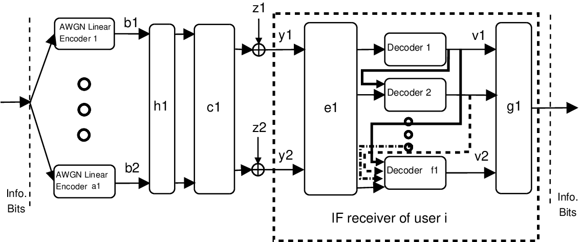
Refer to caption
Fig. 1: Linear pre-processed-IF / Linear pre-processed IF-SIC scheme. Feedback in the receiver is active only when SIC is used.

In [8], a receiver architecture scheme named “integer forcing” was proposed which we briefly recall. For our purposes, it will suffice to only state the achievable rates of IF and a high-level operational description of its elements. The reader is referred to [8] for the derivation, details and proofs, and further to [9, 10] and references therein for implementation considerations.

We follow the derivation of [8] and describe integer forcing over the reals. Channel model (1) can be expressed via its real-valued representation as

[Re⁡(𝐲c)Im⁡(𝐲c)]⏟𝐲=[Re⁡(𝐇c)−Im⁡(𝐇c)Im⁡(𝐇c)Re⁡(𝐇c)]⏟𝐇​[Re⁡(𝐱c)Im⁡(𝐱c)]⏟𝐱+[Re⁡(𝐳c)Im⁡(𝐳c)]⏟𝐳.\displaystyle\underbrace{\begin{bmatrix}{\rm Re}({\bf y}_{c})\\ {\rm Im}({\bf y}_{c})\end{bmatrix}}_{{\bf y}}=\underbrace{\begin{bmatrix}{\rm Re}({\mathbf{H}_{c}})&&-{\rm Im}({\mathbf{H}_{c}})\\ {\rm Im}({\mathbf{H}_{c}})&&{\rm Re}({\mathbf{H}_{c}})\end{bmatrix}}_{\mathbf{H}}\underbrace{\begin{bmatrix}{\rm Re}({\bf x}_{c})\\ {\rm Im}({\bf x}_{c})\end{bmatrix}}_{{\bf x}}+\underbrace{\begin{bmatrix}{\rm Re}({\bf z}_{c})\\ {\rm Im}({\bf z}_{c})\end{bmatrix}}_{{\bf z}}. (10)

This real-valued representation is used in the sequel to derive performance bounds for the complex channel 𝐇c\mathbf{H}_{c}. Note that the dimensions of 𝐇\mathbf{H} are 2​Nr×2​Nt2N_{r}\times 2N_{t}.

It is assumed that information bits are fed into 2​Nt2N_{t} encoders, each of which uses the same linear code that is designed for an AWGN channel.55 5 The effect of the chosen code on the overall performance of IF is discussed in [4]. The latter produces 2​Nt2N_{t} channel inputs (for example, xm{x}_{m} for the mm’th antenna).66 6 For simplicity of notation the time index is suppressed as the block length plays no role in our description. Of course, to approach capacity, one needs to use a long block. At the receiver, a linear equalization matrix 𝐁∈ℝ2​Nt×2​Nr\mathbf{B}\in\mathbb{R}^{2N_{t}\times 2N_{r}} is applied. It is easiest to understand IF by first describing its zero-forcing variant. In this case, 𝐁\mathbf{B} is designed so that the resulting equivalent channel 𝐀=𝐁𝐇\mathbf{A}=\mathbf{B}\mathbf{H} is such that 𝐀∈ℤ2​Nt×2​Nt\mathbf{A}\in\mathbb{Z}^{2N_{t}\times 2N_{t}} is a full-rank integer matrix. In a practical implementation, it may be necessary for the matrix to be full-rank over a finite field ℤp\mathbb{Z}_{p} (where pp is prime) over which the code is defined. Nonetheless, by taking pp large enough, it suffices for 𝐀\mathbf{A} to be invertible over the reals (see Lemma 2 in Appendix A of [11]; see also [10]). This ensures that the output of the channel (without noise) after applying a modulo operation is a valid codeword.

Each of the equalized streams is next passed to a standard (up to the additional element of a modulo operation) AWGN decoder which tries to decode a linear combination of codewords, whose coefficients correspond to a row of 𝐀\mathbf{A}. Finally, after the noise is removed, the original messages are recovered by applying the inverse of 𝐀\mathbf{A}. Thus, for IF equalization to be successful, decoding over all 2​Nt2N_{t} subchannels should be successful and the worst subchannel constitutes a bottleneck. The operation of the receiver is depicted in Figure 1 (where at this stage the linear pre-processing matrix can be considered as the identity matrix, i.e., 𝐏=𝐈\mathbf{P}=\mathbf{I}).

When using minimum mean square error (MMSE) equalization, rather than zero-forcing, the linear equalizer takes the form

𝐁=𝐀𝐇T​(𝐈+𝐇𝐇T)−1,\displaystyle\mathbf{B}=\mathbf{A}\mathbf{H}^{T}\left(\mathbf{I}+\mathbf{H}\mathbf{H}^{T}\right)^{-1}, (11)

and the input to the mm’th decoder is

𝒚eff,m=𝒗m+𝒛eff,m\displaystyle{\boldsymbol{y}}_{\rm eff,m}=\boldsymbol{v}_{m}+\boldsymbol{z}_{\rm eff,m} (12)

where

𝒛eff,m=(𝒃mT​𝐇−𝒂mT)​𝒙+𝒃mT​𝒛.\displaystyle\boldsymbol{z}_{\rm eff,m}=(\boldsymbol{b}_{m}^{T}\mathbf{H}-\boldsymbol{a}_{m}^{T})\boldsymbol{x}+\boldsymbol{b}_{m}^{T}\boldsymbol{z}. (13)

Here, 𝐚mT{\bf a}_{m}^{T} and 𝐛mT{\bf b}_{m}^{T} are the m’th row of 𝐀\mathbf{A} and 𝐁\mathbf{B} respectively. We can define the effective SNR at the mm’th subchannel as

𝖲𝖭𝖱eff​(𝐚m)=(𝒂mT​(𝐈+𝐇T​𝐇)−1​𝒂m)−1,\displaystyle\text{$\mathsf{SNR}$}_{\rm eff}({\bf a}_{m})=\left(\boldsymbol{a}_{m}^{T}(\mathbf{I}+\mathbf{H}^{T}\mathbf{H})^{-1}\boldsymbol{a}_{m}\right)^{-1}, (14)

and the effective rate that can be achieved at the mm’th subchannel as

RIF​(𝐇,𝐚m)\displaystyle R_{\rm IF}(\mathbf{H};{\bf a}_{m}) =12​log⁡(𝖲𝖭𝖱eff​(𝐚m))\displaystyle=\frac{1}{2}\log\left(\text{$\mathsf{SNR}$}_{\rm eff}({\bf a}_{m})\right)
=−12​log⁡(𝒂mT​(𝐈+𝐇T​𝐇)−1​𝒂m).\displaystyle=-\frac{1}{2}\log\left(\boldsymbol{a}_{m}^{T}(\mathbf{I}+\mathbf{H}^{T}\mathbf{H})^{-1}\boldsymbol{a}_{m}\right). (15)

Note that the rate expression (15) is negative when 𝖲𝖭𝖱eff​(𝐚m)<1\text{$\mathsf{SNR}$}_{\rm eff}({\bf a}_{m})<1. Hence, the achievable rate should be understood as the maximum between (15) and zero.

By Theorem 3 in [8], transmission with IF equalization can achieve any rate satisfying R<RIF​(𝐇)R<R_{\rm IF}(\mathbf{H}) where

RIF​(𝐇)=max𝐀∈ℤ2​Nt×2​Ntdet𝐀≠0⁡minm=1,…,2​Nt​2​Nt⋅RIF​(𝐇,𝐚m)\displaystyle R_{\rm IF}(\mathbf{H})=\max_{\begin{subarray}{c}\mathbf{A}\in\mathbb{Z}^{2N_{t}\times 2N_{t}}\\ \det{\mathbf{A}}\neq 0\end{subarray}}\min_{m=1,...,2N_{t}}2N_{t}\cdot R_{\rm IF}(\mathbf{H};{\bf a}_{m})
=max𝐀∈ℤ2​Nt×2​Ntdet𝐀≠0⁡minm=1,…,2​Nt​2​Nt​12​log⁡(𝖲𝖭𝖱eff​(𝐚m))\displaystyle=\max_{\begin{subarray}{c}\mathbf{A}\in\mathbb{Z}^{2N_{t}\times 2N_{t}}\\ \det{\mathbf{A}}\neq 0\end{subarray}}\min_{m=1,...,2N_{t}}2N_{t}\frac{1}{2}\log\left(\text{$\mathsf{SNR}$}_{\rm eff}({\bf a}_{m})\right)
=max𝐀∈ℤ2​Nt×2​Ntdet𝐀≠0⁡minm=1,…,2​Nt​Nt​log⁡(1𝒂mT​(𝐈+𝐇T​𝐇)−1​𝒂m)\displaystyle=\max_{\begin{subarray}{c}\mathbf{A}\in\mathbb{Z}^{2N_{t}\times 2N_{t}}\\ \det{\mathbf{A}}\neq 0\end{subarray}}\min_{m=1,...,2N_{t}}N_{t}\log\left(\frac{1}{\boldsymbol{a}_{m}^{T}(\mathbf{I}+\mathbf{H}^{T}\mathbf{H})^{-1}\boldsymbol{a}_{m}}\right)
=Nt​log⁡(min𝐀∈ℤ2​Nt×2​Ntdet𝐀≠0⁡maxm=1,…,2​Nt⁡(𝒂mT​(𝐈+𝐇T​𝐇)−1​𝒂m))−1\displaystyle=N_{t}\log\left(\min_{\begin{subarray}{c}\mathbf{A}\in\mathbb{Z}^{2N_{t}\times 2N_{t}}\\ \det{\mathbf{A}}\neq 0\end{subarray}}\max_{m=1,...,2N_{t}}\left(\boldsymbol{a}_{m}^{T}(\mathbf{I}+\mathbf{H}^{T}\mathbf{H})^{-1}\boldsymbol{a}_{m}\right)\right)^{-1}
=−Nt​log⁡(min𝐀∈ℤ2​Nt×2​Ntdet𝐀≠0⁡maxm=1,…,2​Nt⁡(𝒂mT​(𝐈+𝐇T​𝐇)−1​𝒂m)).\displaystyle=-N_{t}\log\left(\min_{\begin{subarray}{c}\mathbf{A}\in\mathbb{Z}^{2N_{t}\times 2N_{t}}\\ \det{\mathbf{A}}\neq 0\end{subarray}}\max_{m=1,...,2N_{t}}\left(\boldsymbol{a}_{m}^{T}(\mathbf{I}+\mathbf{H}^{T}\mathbf{H})^{-1}\boldsymbol{a}_{m}\right)\right). (16)

The achievable rate of IF may also be described via the successive minima of a lattice associated with the channel matrix as we now recall. Any channel can be described via its SVD

𝐇=𝐔​𝚺​𝐕T.\displaystyle\mathbf{H}=\mathbf{U}\mathbf{\Sigma}\mathbf{V}^{T}. (17)

Using (17), the following decomposition is readily obtained

(𝐈+𝐇T​𝐇)−1=𝐕𝐃−1​𝐕T,\displaystyle(\mathbf{I}+\mathbf{H}^{T}\mathbf{H})^{-1}=\mathbf{V}\mathbf{D}^{-1}\mathbf{V}^{T}, (18)

where 𝐃=𝐈+ΣT​Σ\mathbf{D}=\mathbf{I}+{\Sigma}^{T}{\Sigma}. It follows that (15) may be rewritten as (Theorem 4 in [8])

RIF​(𝐇,𝐚m)\displaystyle R_{\rm IF}(\mathbf{H};{\bf a}_{m}) =−12log(∥𝐃−1/2𝐕T𝐚m∥2)\displaystyle=-\frac{1}{2}\log\left(\|\mathbf{D}^{-1/2}\mathbf{V}^{T}{\bf a}_{m}\|^{2}\right)
≜Rm,IF​(𝐃,𝐕),\displaystyle\triangleq R_{m,\rm IF}(\mathbf{D},\mathbf{V}), (19)

where in the last equation the dependence on the choice of 𝐀\mathbf{A} is left implicit. Let Λ\Lambda be the lattice spanned by 𝐆=𝐃−1/2𝐕T\mathbf{G}=\mathbf{D}^{-1/2}\mathbf{V}^{T}and recall the definition of successive minima.

Definition 1.

Let Λ⁡(𝐆)\Lambda(\mathbf{G}) be a lattice spanned by the full-rank matrix 𝐆∈ℝK×K\mathbf{G}\in\mathbb{R}^{K\times K}. For k=1,…,Kk=1,...,K, we define the kk’th successive minimum as

λk​(𝐆)≜inf{r:dim⁡(span⁡(Λ⁡(𝐆)∩ℬK​(r)))≥k}\displaystyle\lambda_{k}(\mathbf{G})\triangleq\inf\left\{r:{\rm dim}\left({\rm span}\left(\Lambda(\mathbf{G})\cap\mathcal{B}_{K}(r)\right)\right)\geq k\right\} (20)

where ℬK​(r)={𝐱∈ℝK:‖𝐱‖≤r}\mathcal{B}_{K}(r)=\left\{{\bf x}\in\mathbb{R}^{K}:\|{\bf x}\|\leq r\right\} is the closed ball of radius rr around 𝟎{\bf 0}. In words, the kk-th successive minimum of a lattice is the minimal radius of a ball centered around 𝟎{\bf 0} that contains kk linearly independent lattice points.

Thus, the maximal rate achievable with integer-forcing equalization (16) may be written as

RIF​(𝐇)\displaystyle R_{\rm IF}(\mathbf{H}) =RIF​(𝐃,𝐕)\displaystyle=R_{\rm IF}(\mathbf{D},\mathbf{V})
=−Nt​log⁡(λ2​Nt2​(Λ))\displaystyle=-N_{t}\log\left(\lambda_{2N_{t}}^{2}(\Lambda)\right)
=Nt​log⁡(1λ2​Nt2​(Λ)).\displaystyle=N_{t}\log\left(\frac{1}{\lambda_{2N_{t}}^{2}(\Lambda)}\right). (21)

III-B Integer-Forcing Equalization With Successive Interference Cancellation

We also consider a version of IF equalization incorporating successive interference cancellation. We will refer to it as IF-SIC.77 7 We note that IF-SIC may in general allow using different rates per stream as stated in Theorem 5 in [10]. We nevertheless assume throughout that all streams are encoded via an identical linear code and hence have the same rate. We state only the achievable rates of IF-SIC and an operational description of its elements. The reader is referred to [12] for the derivation, details and proofs.

For a given choice of integer matrix 𝐀\mathbf{A}, let 𝐋\mathbf{L} be defined by the following Cholesky decomposition

𝐀​(𝐈+𝐇T​𝐇)−1​𝐀T\displaystyle\mathbf{A}\left(\mathbf{I}+\mathbf{H}^{T}\mathbf{H}\right)^{-1}\mathbf{A}^{T} =𝐀𝐕𝐃−1​𝐕T​𝐀T\displaystyle=\mathbf{A}\mathbf{V}\mathbf{D}^{-1}\mathbf{V}^{T}\mathbf{A}^{T}
=𝐋𝐋T.\displaystyle=\mathbf{L}\mathbf{L}^{T}. (22)

Denoting by ℓm,m\ell_{m,m} the diagonal entries of 𝐋\mathbf{L}, IF-SIC can achieve (see [12]) any rate satisfying R<RIF−SIC​(𝐇)R<R_{\rm IF-SIC}(\mathbf{H}) where

RIF−SIC​(𝐇)\displaystyle R_{\rm IF-SIC}(\mathbf{H}) =RIF−SIC​(𝐃,𝐕)\displaystyle=R_{\rm IF-SIC}(\mathbf{D},\mathbf{V})
=2​Nt⋅12​max𝐀​minm=1,…,2​Nt​log⁡(1ℓm,m2),\displaystyle=2N_{t}\cdot\frac{1}{2}\max_{\mathbf{A}}\min_{m=1,...,2N_{t}}\log\left(\frac{1}{\ell_{m,m}^{2}}\right), (23)

and the maximization is over all full-rank 2​Nt×2​Nt2N_{t}\times 2N_{t} integer matrices.88 8 We note that since we choose to work with equal-rate streams, the constraints on the achievable rate tuples of IF with SIC, as stated in Theorem 2 of [12], play no role in the present work.

We describe the operation of the IF-SIC receiver, adopting the nomenclature of [12]. We note that we describe the MMSE-GDFE version of IF-SIC, as given in Appendix A of [12], rather than its noise-prediction variant. First, calculate:

  1. 1.

    The optimal integer matrix 𝐀\mathbf{A}, i.e., the matrix maximizing (23).

  2. 2.

    The covariance matrix (22) of the effective noise (see (14)) that arises when using the equalization matrix 𝐁\mathbf{B} as given in (11).

  3. 3.

    The optimal SIC matrix 𝐒\mathbf{S} as:

    𝐒=diag⁡(ℓ11,…,ℓM​M)⋅𝐋−1.\displaystyle\mathbf{S}={\rm diag}(\ell_{11},...,\ell_{MM})\cdot\mathbf{L}^{-1}. (24)
  4. 4.

    The optimal combined linear front-end processing matrix:

    𝐁~\displaystyle\widetilde{\mathbf{B}} =\displaystyle= 𝐒𝐁\displaystyle\mathbf{S}\mathbf{B} (25)
    =\displaystyle= 𝐒𝐀𝐇T​(𝐈+𝐇𝐇T)−1.\displaystyle\mathbf{S}\mathbf{A}\mathbf{H}^{T}\left(\mathbf{I}+\mathbf{H}\mathbf{H}^{T}\right)^{-1}.

The operation of the receiver is depicted in Figure 1 where the feedback depicted in the receiver is now active, and where now 𝐁\mathbf{B} is to be understood as 𝐁~\widetilde{\mathbf{B}}. Note that this change of linear post-processing is essential to guarantee that the resulting noise variance is minimized. The outputs of decoders 1,…,m−11,\ldots,m-1 are multiplied by Sm,1,…,Sm,m−1S_{m,1},\ldots,S_{m,m-1}, respectively, and are then subtracted from the input to decoder mm, thereby performing SIC.

III-C Linear Pre-Processed Integer Forcing

III-C1 Motivating example: Performance comparison of linear MMSE and IF receivers

As a motivating example, following Remark 1, we compare the performance of linear MMSE and IF equalizers over a specific ensemble of channels defined over ℍ⁡(C=8,Nt=2)\mathbb{H}(C=8,N_{t}=2). Specifically, we consider a “normalized” 2×22\times 2 Rayleigh fading ensemble, where the capacity is fixed to C=8C=8 bits. The ensemble is generated by drawing a 2×22\times 2 channel matrix with i.i.d. circularly symmetric complex Gaussian entries and then scaling the matrix (multiplying it by a value that we find by numerical search) such that the mutual information equals 88 bits.99 9 Note that in this ensemble, the probability of channels corresponding to Nr≠2N_{r}\neq 2 is zero.

Refer to caption
Fig. 2: Approximate probability density functions (based on Monte Carlo simulation) of the rates achievable with the linear MMSE receivers over a Rayleigh 2×22\times 2 MIMO channel normalized to C=8C=8 bits.

Figure 2 depicts the probability density function of the rate achieved for this ensemble when using linear MMSE and IF receivers. Since linear MMSE equalization is a special case of IF (setting 𝐀=𝐈\mathbf{A}=\mathbf{I}), as expected IF displays improved performance.

The real strength of IF lies however in the behavior of the “tail”. For conventional linear equalizers, bad channels correspond to ill-conditioned matrices. An extreme case is the following channel

𝐇c,WORST=28−1​[1000].\displaystyle\mathbf{H}_{\rm c,WORST}=\sqrt{2^{8}-1}\begin{bmatrix}1&0\\ 0&0\end{bmatrix}. (26)

In this case, the data stream sent from the second antenna is completely lost when transmitted over the channel. Clearly, in this example, no receiver (including maximum likelihood) will be able to recover the lost data stream and thus the achievable rate of both linear and IF equalization is also zero.

Consider now the channel 𝐇c,WORST⋅𝐏c\mathbf{H}_{\rm c,WORST}\cdot\mathbf{P}_{c} where 𝐏c\mathbf{P}_{c} is a unitary matrix. As the singular values remain unchanged, it is clear that the channel remains ill-conditioned and hence a linear receiver (not allowing for a modulo operation) will still suffer from poor performance. On the other hand, the IF receiver performs well even over ill-conditioned MIMO channels, and in fact, the performance of the IF receiver for the channel (26) is good for “most” pre-processing matrices as illustrated next.

III-C2 Linear pre-processing ensemble and resulting performance

The transmission scheme we analyze consists of applying a unitary pre-processing matrix at the transmitter and IF equalization (either with or without SIC) at the receiver, as depicted in Figure 1. Applying linear pre-processing may be viewed as generating a “virtual” channel 𝐇~c=𝐇c​𝐏c\widetilde{\mathbf{H}}_{c}=\mathbf{H}_{c}\mathbf{P}_{c} over which transmission takes place. We restrict ourselves to unitary linear pre-processing matrices in order to keep the transmission power unchanged.

Throughout this paper, we assume that the linear pre-processing matrix 𝐏c\mathbf{P}_{c} is drawn from what is referred to as the “circular unitary ensemble” (CUE). The ensemble is defined by the unique distribution on unitary matrices that is invariant under left and right unitary transformations (Theorem 8.3 in [13]). In other words, the ensemble amounts to inducing the Haar measure on the unitary group of degree NtN_{t}.1010 10 An explanation on how to generate matrices belonging to the CUE can be found in, e.g., [14].

Remark 3.

While in general the transformation 𝐏c{\mathbf{P}}_{c} implies joint processing at the encoders, we note that in some natural statistical scenarios, including that of an i.i.d. Rayleigh fading environment, the random transformation is actually performed by nature.1111 11 This follows since the left and right singular vector matrices of the an i.i.d. Gaussian matrix 𝐇c\mathbf{H}_{c} are equal to the eigenvector matrices of the Wishart ensembles 𝐇c​𝐇cH\mathbf{H}_{c}\mathbf{H}_{c}^{H} and 𝐇cH​𝐇c\mathbf{H}^{H}_{c}\mathbf{H}_{c}, respectively. The latter are known to be CUE (Haar) distributed. See, e.g., Chapter 4.6 in [15]. In such settings, our analysis holds even when the transmitters are distributed as in a multiple-access scenario.

Figure 3 compares the achievable rates of the linear MMSE and IF receivers over the singular channel (26), when applying random CUE pre-processing. As can be seen, the achievable rate of IF is high for most pre-processing matrices, achieving a large fraction of CC with high probability.

Refer to caption
Fig. 3: Approximate probability density functions (based on Monte Carlo simulation) of the rates achievable with the linear MMSE and IF receivers over the channel (26), when applying a random linear pre-processing matrix drawn from the CUE.

III-C3 Properties of CUE pre-processing

The SVD of the effective channel resulting from pre-processing is given by

𝐇c​𝐏c=𝐔c​𝚺c​𝐕cH​𝐏c.\displaystyle\mathbf{H}_{c}{\mathbf{P}}_{c}=\mathbf{U}_{c}\mathbf{\Sigma}_{c}{\mathbf{V}}_{c}^{H}{\mathbf{P}}_{c}. (27)

Since 𝐕cH​𝐏c{\mathbf{V}}_{c}^{H}{\mathbf{P}}_{c} is equal in distribution to 𝐏c{\mathbf{P}}_{c}, for the sake of computing outage probabilities, we may simply assume that 𝐕cH{\mathbf{V}}_{c}^{H} (and also 𝐕c{\mathbf{V}}_{c}) is drawn from the CUE.

We note that the eigenvalue decomposition of the equivalent real channel can be written as

(𝐈+𝐇T​𝐇)−1=𝐕𝐃−1​𝐕T,\displaystyle(\mathbf{I}+\mathbf{H}^{T}\mathbf{H})^{-1}=\mathbf{V}\mathbf{D}^{-1}\mathbf{V}^{T}, (28)

where

𝐕=[Re⁡(𝐕c)−Im⁡(𝐕c)Im⁡(𝐕c)Re⁡(𝐕c)].\displaystyle{\mathbf{V}}=\begin{bmatrix}{\rm Re}({\mathbf{V}_{c}})&&-{\rm Im}({\mathbf{V}_{c}})\\ {\rm Im}({\mathbf{V}_{c}})&&{\rm Re}({\mathbf{V}_{c}})\end{bmatrix}. (29)

and

𝐃=[𝐃c𝟎𝟎𝐃c].\displaystyle\mathbf{D}=\begin{bmatrix}\mathbf{D}_{c}&&\mathbf{0}\\ \mathbf{0}&&\mathbf{D}_{c}\end{bmatrix}. (30)

Further, the rates of IF, with or without SIC, for such a channel come in pairs.

Denoting the gap-to-capacity by Δ​C\Delta C, we may therefore rewrite the worst-case IF outage probability as defined in (6) as

Pout,IFWC​(C,C−Δ​C)=sup𝐃∈𝔻⁡(C,2​Nt)Pr⁡(RIF​(𝐃,𝐕)<C−Δ​C)\displaystyle P^{\rm WC}_{\rm out,IF}\left(C,C-\Delta C\right)=\sup_{\mathbf{D}\in\mathbb{D}(C;2N_{t})}{\rm Pr}\left(R_{\rm IF}(\mathbf{D},\mathbf{V})<C-\Delta C\right) (31)

where we define 𝔻⁡(C,2​Nt)\mathbb{D}(C;2N_{t}) as the set of all 2​Nt×2​Nt2N_{t}\times 2N_{t} diagonal matrices 𝐃\mathbf{D}, with diagonal elements appearing in pairs, such that det(𝐃)=2C\det\left(\mathbf{D}\right)=2^{C}.

Another property we use in the sequel is the following. Denote by dc,id_{c,i} the diagonal entries of 𝐃c\mathbf{D}_{c}. Then

2C\displaystyle 2^{C} =2logdet(𝐈Nt×Nt+𝐇cH𝐇c)\displaystyle=2^{\log\det\left(\mathbf{I}_{N_{t}\times N_{t}}+\mathbf{H}_{c}^{H}\mathbf{H}_{c}\right)}
=det(𝐕c​𝐃c​𝐕cH)\displaystyle=\det\left(\mathbf{V}_{c}\mathbf{D}_{c}\mathbf{V}_{c}^{H}\right)
=∏i=1Ntdc,i.\displaystyle=\prod_{i=1}^{N_{t}}d_{c,i}. (32)

Denoting by did_{i} the diagonal entries of 𝐃\mathbf{D}, we similarly have

2C\displaystyle 2^{C} =212​log​det(𝐈Nt×Nt+𝐇T​𝐇)\displaystyle=2^{\frac{1}{2}\log\det\left(\mathbf{I}_{N_{t}\times N_{t}}+\mathbf{H}^{T}\mathbf{H}\right)}
=det(𝐕⋅𝐃⋅𝐕T)\displaystyle=\sqrt{\det\left(\mathbf{V}\cdot\mathbf{D}\cdot\mathbf{V}^{T}\right)}
=∏i=12​Ntdi.\displaystyle=\prod_{i=1}^{2N_{t}}\sqrt{d_{i}}. (33)

From (30) we observe that since the singular values of the real channel come in pairs, we have

∏i=12​Ntdi=∏i=1Ntdc,i=2C.\displaystyle\prod_{i=1}^{2N_{t}}\sqrt{d_{i}}=\prod_{i=1}^{N_{t}}d_{c,i}=2^{C}. (34)

We denote dmin=mini⁡did_{\min}=\displaystyle\min_{i}d_{i} and dmax=maxi⁡did_{\max}=\displaystyle\max_{i}d_{i}.

The following lemma will prove useful in characterizing the performance of CUE pre-processed IF. It relates the outage probability of CUE pre-processed IF to that arising when the pre-processing is performed using the circular real ensemble (CRE).1212 12 The CRE is defined analogously to the CUE for the case of real orthonormal matrices. That is, the ensemble is defined by the unique distribution on orthonormal matrices that is invariant under left and right orthonormal transformations.

Lemma 1.

Let 𝐎\mathbf{O} be a real 2​Nt×2​Nt2N_{t}\times 2N_{t} matrix drawn from the CRE. Further, let 𝐚\mathbf{a} be a 2​Nt×12N_{t}\times 1 vector of integers. When applying a random complex linear pre-processing matrix 𝐕c\mathbf{V}_{c} that is drawn from the CUE (inducing a real-valued orthogonal pre-processing matrix 𝐕\mathbf{V}), we have that ‖𝐃1/2​𝐕𝐚‖\left\|\mathbf{D}^{1/2}\mathbf{V}{\bf a}\right\| and ‖𝐃1/2​𝐎𝐚‖\left\|\mathbf{D}^{1/2}\mathbf{O}{\bf a}\right\| are equal in distribution.

Proof.

See Appendix A. ∎

IV Bounds on the outage probability of CUE pre-processed Integer-Forcing

IV-A Derivation of Upper Bounds

Define the dual lattice Λ∗\Lambda^{*} which is spanned by the matrix

(𝐆T)−1=𝐃1/2​𝐕T.\displaystyle(\mathbf{G}^{T})^{-1}=\mathbf{D}^{1/2}\mathbf{V}^{T}. (35)

Recall that the rate of IF is given by (21). Now, the successive minima of Λ\Lambda and Λ∗\Lambda^{*} are related by (Theorem 2.4 in[16])

λ1​(Λ∗)2​λ2​Nt​(Λ)2≤2​Nt+34​γ¯2​Nt2,\displaystyle\lambda_{1}(\Lambda^{*})^{2}\lambda_{2N_{t}}(\Lambda)^{2}\leq\frac{2N_{t}+3}{4}{\bar{\gamma}_{2N_{t}}}^{2}, (36)

where γ¯2​Nt\bar{\gamma}_{2N_{t}} is a ‘‘monotonized” Hermite’s constant as defined next.1313 13 In [17], Theorem 2.1, another bound for the relation between the successive minima of Λ\Lambda and Λ∗\Lambda^{*} is given. This bound is tighter for very large dimensions (it increases with n2n^{2}, whereas (36) increases with n3n^{3}). However, (36) has better constants and the cross between these expressions occurs only at n=254n=254. Hermite’s constant is known only for dimensions 1−81-8 and 2424. Since it has been never proved that γ2​Nt\gamma_{2N_{t}} is monotonically increasing, we define

γ¯2​Nt=max⁡{γi:1≤i≤2​Nt}.\displaystyle\bar{\gamma}_{2N_{t}}=\max\left\{\gamma_{i}:1\leq i\leq 2N_{t}\right\}. (37)

The tightest known upper bound for Hermite’s constant, as derived in [18], is

γ2​Nt≤(2π)​Γ​(2+Nt)1/Nt.\displaystyle\gamma_{2N_{t}}\leq\left(\frac{2}{\pi}\right)\Gamma\left(2+N_{t}\right)^{1/N_{t}}. (38)

Since this is an increasing function of NtN_{t}, it follows that γ¯2​Nt\bar{\gamma}_{2N_{t}} is smaller than the r.h.s. of (38).1414 14 In the sequel we use the known values of Hermite’s constant when possible, i.e. for Nt=2,3,4N_{t}=2,3,4. For other dimensions, we use this bound. Combining the latter with the exact values of the Hermite constant for dimensions for which it is known, we may lower bound the achievable rates of IF via the dual lattice as follows

RIF​(𝐃,𝐕)≥Nt​log⁡(λ12​(Λ∗)α⁡(Nt)),\displaystyle R_{\rm IF}(\mathbf{D},\mathbf{V})\geq N_{t}\log\left(\frac{\lambda_{1}^{2}(\Lambda^{*})}{\alpha(N_{t})}\right), (39)

where

α⁡(Nt)={2​Nt+34​γ2​Nt2,Nt=2,3,4,122​Nt+34​(2π​Γ​(2+Nt)1/Nt)2,otherwise.\displaystyle\alpha(N_{t})=\begin{cases}\frac{2N_{t}+3}{4}\gamma_{2N_{t}}^{2},&N_{t}=2,3,4,12\\ \frac{2N_{t}+3}{4}\left(\frac{2}{\pi}\Gamma\left(2+N_{t}\right)^{1/N_{t}}\right)^{2},&{\rm otherwise}\end{cases}. (40)

Hence,

Pr⁡(RIF​(𝐃,𝐕)<C−Δ​C)\displaystyle{\rm Pr}\left(R_{\rm IF}(\mathbf{D},\mathbf{V}\right)<C-\Delta C)
≤Pr⁡(Nt​log⁡(λ12​(Λ∗)α⁡(Nt))<C−Δ​C)\displaystyle\leq{\rm Pr}\left(N_{t}\log\left(\frac{\lambda_{1}^{2}(\Lambda^{*})}{\alpha(N_{t})}\right)<C-\Delta C\right)
=Pr⁡(λ12​(Λ∗)<2C−Δ​CNt​α​(Nt)).\displaystyle={\rm Pr}\left(\lambda_{1}^{2}(\Lambda^{*})<2^{\frac{C-\Delta C}{N_{t}}}\alpha(N_{t})\right). (41)

The next lemma provides an upper bound on the outage probability as a function of the gap-to-capacity Δ​C\Delta C, the capacity CC, and dmind_{\min} (as well as the number of transmit antennas). Denote

𝔸⁡(β,d,2​Nt)≜{𝐚∈ℤ2​Nt:0<‖𝐚‖<βd}.\displaystyle\mathbb{A}({\beta},d;2N_{t})\triangleq\left\{{\bf a}\in\mathbb{Z}^{2N_{t}}:0<\|{\bf a}\|<\sqrt{\frac{{\beta}}{d}}\right\}. (42)
Lemma 2.

For any complex Gaussian MIMO channel with NtN_{t} transmit antennas and with white-input mutual information CC, i.e., 𝐃∈𝔻⁡(C,2​Nt)\mathbf{D}\in\mathbb{D}(C;2N_{t}), and for 𝐕c\mathbf{V}_{c} drawn from the CUE (inducing a real-valued orthogonal pre-processing matrix 𝐕\mathbf{V}), the outage probability of integer forcing is upper bounded by

Pr⁡(RIF​(𝐃,𝐕)<C−Δ​C)\displaystyle{\rm Pr}\left(R_{\rm IF}(\mathbf{D},\mathbf{V}\right)<C-\Delta C)
≤∑𝐚∈𝔸⁡(β,dmin,2​Nt)2​Nt​(2C−Δ​CNt​α​(Nt))Nt−1/2‖𝐚‖2​Nt−1​2C​2dmin,\displaystyle\leq\sum_{{\bf a}\in\mathbb{A}({\beta},d_{\min};2N_{t})}\frac{2N_{t}\left(2^{\frac{C-\Delta C}{N_{t}}}\alpha(N_{t})\right)^{N_{t}-1/2}}{\|{\bf a}\|^{2N_{t}-1}2^{C}\frac{2}{\sqrt{d_{\min}}}}, (43)

where

β=2C−Δ​CNt​α​(Nt).\displaystyle{\beta}=2^{\frac{C-\Delta C}{N_{t}}}\alpha(N_{t}). (44)
Remark 4.

The summation in (43) may be greater than 1 for certain values of CC and Δ​C\Delta C. Obviously, one may take the minimum between this lemma and 11 when bounding the outage probability.

Proof.

For a given β>0{\beta}>0, let us upper bound the probability Pr⁡(λ12​(Λ∗)<β){\rm Pr}\left(\lambda_{1}^{2}(\Lambda^{*})<{{\beta}}\right) or equivalently Pr⁡(λ1​(Λ∗)<β){\rm Pr}\left(\lambda_{1}(\Lambda^{*})<\sqrt{{\beta}}\right). Noting that the event {λ1(Λ∗)<β}\left\{\lambda_{1}(\Lambda^{*})<\sqrt{{\beta}}\right\} is equivalent to the event

⋃𝐚∈ℤ2​Nt∖{𝟎}{||𝐃1/2𝐕𝐚||<β}\displaystyle\bigcup_{\mathbf{a}\in{\mathbb{Z}^{2N_{t}}\setminus\{{\bf 0}\}}}\left\{||\mathbf{D}^{1/2}\mathbf{V}\mathbf{a}||<\sqrt{{\beta}}\right\} (45)

and applying the union bound gives

Pr⁡(λ1​(Λ∗)<β)\displaystyle{\rm Pr}\left(\lambda_{1}(\Lambda^{*})<\sqrt{{\beta}}\right) ≤∑𝐚∈ℤ2​Nt∖{𝟎}Pr⁡(‖𝐃1/2​𝐕𝐚‖<β)\displaystyle\leq\sum_{{\bf a}\in\mathbb{Z}^{2N_{t}}\setminus\{{\bf 0}\}}{\rm Pr}\left(\|\mathbf{D}^{1/2}\mathbf{V}{\bf a}\|<\sqrt{{\beta}}\right)
=∑𝐚∈𝔸⁡(β,dmin,2​Nt)Pr⁡(‖𝐃1/2​𝐕T​𝐚‖<β),\displaystyle=\sum_{{\bf a}\in\mathbb{A}({\beta},d_{\min};2N_{t})}{\rm Pr}\left(\|\mathbf{D}^{1/2}\mathbf{V}^{T}{\bf a}\|<\sqrt{{\beta}}\right), (46)

where the equality in (46) follows since whenever ‖𝐚‖⋅dmin≥β\|{\bf a}\|\cdot\sqrt{d_{\min}}\geq\sqrt{{\beta}}, we have that Pr⁡(‖𝐃1/2​𝐕𝐚‖<β)=0{\rm Pr}\left(\|\mathbf{D}^{1/2}\mathbf{V}{\bf a}\|<\sqrt{{\beta}}\right)=0.

Let 𝒮\mathcal{S} denote the unit sphere of dimension 2​Nt2N_{t}, i.e.,

𝒮={(x1,x2,⋯,x2​Nt):x12+x22+⋯+x2​Nt2=1}.\displaystyle\mathcal{S}=\left\{(x_{1},x_{2},\cdots,x_{2N_{t}}):x_{1}^{2}+x_{2}^{2}+\cdots+x_{2N_{t}}^{2}=1\right\}. (47)

By Lemma 1

Pr⁡(‖𝐃1/2​𝐕𝐚‖<β)=Pr⁡(‖𝐃1/2​𝐎𝐚‖<β).\displaystyle{\rm Pr}\left(\|\mathbf{D}^{1/2}\mathbf{V}{\bf a}\|<\sqrt{{\beta}}\right)={\rm Pr}\left(\|\mathbf{D}^{1/2}\mathbf{O}\mathbf{a}\|<\sqrt{{\beta}}\right). (48)

Let 𝐨‖𝐚‖∼Unif⁡(𝒮⋅‖𝐚‖){\bf o}_{\|{\bf a}\|}\sim{\rm Unif}(\mathcal{S\cdot\|\mathbf{a}\|}), and note that 𝐎𝐚\mathbf{O}\mathbf{a} is equal in distribution to 𝐨‖𝐚‖{\bf o}_{\|{\bf a}\|}. It follows that

Pr⁡(‖𝐃1/2​𝐕𝐚‖<β)=Pr⁡(‖𝐃1/2​𝐨‖𝐚‖‖<β).\displaystyle{\rm Pr}\left(\|\mathbf{D}^{1/2}\mathbf{V}{\bf a}\|<\sqrt{{\beta}}\right)={\rm Pr}\left(\|\mathbf{D}^{1/2}{\bf o}_{\|{\bf a}\|}\|<\sqrt{{\beta}}\right). (49)

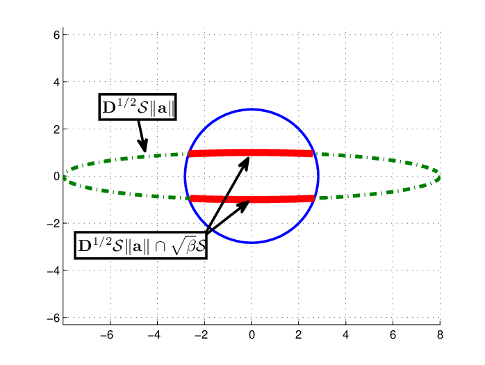
Now the probability appearing on the r.h.s. of (49) has a simple geometric interpretation. Define an ellipsoid with axes xi=di⋅‖𝐚‖x_{i}=\sqrt{d_{i}}\cdot\|{\bf a}\| and denote its surface area by L⁡(x1,x2,…,x2​Nt)L(x_{1},x_{2},...,x_{2N_{t}}). Then, the r.h.s. of (49) is the ratio of the part of the surface area of an ellipsoid that lies inside a sphere of radius β\sqrt{{\beta}} (denoted by CAPell​(x1,x2,…,x2​Nt){\rm CAP_{\rm ell}}(x_{1},x_{2},...,x_{2N_{t}})) and the total surface area of the ellipsoid. This is illustrated in Figure 4 for the case of two real dimensions. We may rewrite (49) as

Pr⁡(‖𝐃1/2​𝐨‖𝐚‖‖<β)\displaystyle{\rm Pr}\left(\|\mathbf{D}^{1/2}{\bf o}_{\|{\bf a}\|}\|<\sqrt{{\beta}}\right) =|𝐃1/2​𝒮⋅‖𝐚‖∩β​𝒮||𝐃1/2​‖𝐚‖​𝒮|\displaystyle=\frac{|\mathbf{D}^{1/2}\mathcal{S}\cdot\|{\bf a}\|\cap\sqrt{{\beta}}\mathcal{S}|}{\left|\mathbf{D}^{1/2}\|{\bf a}\|\mathcal{S}\right|}
=CAPell​(x1,x2,…,x2​Nt)L⁡(x1,x2,…,x2​Nt).\displaystyle=\frac{{\rm CAP_{\rm ell}}(x_{1},x_{2},...,x_{2N_{t}})}{L(x_{1},x_{2},...,x_{2N_{t}})}. (50)

Neither the numerator nor the denominator of (50) has a closed-form expression. In order to upper bound this ratio, we upper bound the numerator CAPell​(x1,x2,…,x2​Nt)\rm CAP_{\rm ell}(x_{1},x_{2},...,x_{2N_{t}}) and lower bound the denominator (the surface area of the ellipsoid). Using inequality (4.3) in [19] (see also inequality (57) and historical account in [20]), we have

L⁡(x1,…,x2​Nt)\displaystyle L(x_{1},...,x_{2N_{t}}) >Vol⁡(ℬ2​Nt​(1))​‖𝐚‖2​Nt​∏i=12​Ntdi​∑i=12​Nt1‖𝐚‖​di\displaystyle>{\rm Vol}(\mathcal{B}_{2N_{t}}(1))\|{\bf a}\|^{2N_{t}}\prod_{i=1}^{2N_{t}}{\sqrt{d_{i}}}\sum_{i=1}^{2N_{t}}{\frac{1}{\|{\bf a}\|\sqrt{d_{i}}}}
≥Vol⁡(ℬ2​Nt​(1))​‖𝐚‖2​Nt−1​2C​2dmin\displaystyle\geq{\rm Vol}(\mathcal{B}_{2N_{t}}(1))\|{\bf a}\|^{2N_{t}-1}2^{C}\frac{2}{\sqrt{d_{\min}}}
≜L¯​(x1,x2,…,x2​Nt),\displaystyle\triangleq\underline{L}(x_{1},x_{2},...,x_{2N_{t}}), (51)

where ℬ2​Nt​(1)\mathcal{B}_{2N_{t}}(1) is a unit ball of dimension 2​Nt2N_{t}, and

Vol⁡(ℬ2​Nt​(1))=πNtΓ⁡(1+Nt)\displaystyle{\rm Vol}(\mathcal{B}_{2N_{t}}(1))=\frac{\pi^{N_{t}}}{\Gamma(1+N_{t})} (52)

is its volume.

As an upper bound for the numerator, we take the entire surface area of a sphere of radius β\sqrt{{\beta}}, which is given by

A2​Nt​(β)=2​Nt​πNtΓ⁡(1+Nt)​β2​Nt−1.\displaystyle A_{2N_{t}}(\sqrt{{\beta}})=2N_{t}\frac{\pi^{N_{t}}}{\Gamma(1+N_{t})}\sqrt{{\beta}}^{2N_{t}-1}. (53)

We thus have

CAPell​(x1,x2,…,x2​Nt)\displaystyle\rm CAP_{\rm ell}(x_{1},x_{2},...,x_{2N_{t}}) ≤A2​Nt​(β)\displaystyle\leq A_{2N_{t}}(\sqrt{{\beta}})
≜CAPell¯​(β).\displaystyle\triangleq{\overline{\rm CAP_{\rm ell}}(\sqrt{{\beta}})}. (54)
Refer to caption
Fig. 4: Illustration of the geometric objects appearing in (50).

We may therefore bound (50) by

Pr⁡(‖𝐃1/2​𝐨‖𝐚‖‖<β)≤CAPell¯​(β)L¯​(x1,x2,…,x2​Nt).\displaystyle{\rm Pr}\left(\|\mathbf{D}^{1/2}{\bf o}_{\|{\bf a}\|}\|<\sqrt{{\beta}}\right)\leq\frac{\overline{\rm CAP_{\rm ell}}(\sqrt{{\beta}})}{\underline{L}(x_{1},x_{2},...,x_{2N_{t}})}. (55)

Substituting (51), (54) into (55) yields

∑𝐚∈𝔸⁡(β,dmin,2​Nt)Pr⁡(‖𝐃1/2​𝐨‖𝐚‖‖<β)\displaystyle\sum_{{\bf a}\in\mathbb{A}({\beta},d_{\min};2N_{t})}{\rm Pr}\left(\|\mathbf{D}^{1/2}{\bf o}_{\|{\bf a}\|}\|<\sqrt{{\beta}}\right)
≤∑𝐚∈𝔸⁡(β,dmin,2​Nt)2​Nt​πNtΓ⁡(1+Nt)​β2​Nt−1πNtΓ⁡(1+Nt)​‖𝐚‖2​Nt−1​2C​2dmin\displaystyle\leq\sum_{{\bf a}\in\mathbb{A}({\beta},d_{\min};2N_{t})}\frac{2N_{t}\frac{\pi^{N_{t}}}{\Gamma(1+N_{t})}\sqrt{{\beta}}^{2N_{t}-1}}{\frac{\pi^{N_{t}}}{\Gamma(1+N_{t})}\|{\bf a}\|^{2N_{t}-1}2^{C}\frac{2}{\sqrt{d_{\min}}}}
=∑𝐚∈𝔸⁡(β,dmin,2​Nt)2​Nt​β2​Nt−1‖𝐚‖2​Nt−1​2C​2dmin.\displaystyle=\sum_{{\bf a}\in\mathbb{A}({\beta},d_{\min};2N_{t})}\frac{2N_{t}\sqrt{{\beta}}^{2N_{t}-1}}{\|{\bf a}\|^{2N_{t}-1}2^{C}\frac{2}{\sqrt{d_{\min}}}}. (56)

Substituting β=2C−Δ​CNt​α​(Nt){\beta}=2^{\frac{C-\Delta C}{N_{t}}}\alpha(N_{t}), we finally arrive at

Pr⁡(RIF​(𝐃,𝐕)<C−Δ​C)\displaystyle{\rm Pr}\left(R_{\rm IF}(\mathbf{D},\mathbf{V})<C-\Delta C\right)
≤∑𝐚∈𝔸⁡(β,dmin,2​Nt)Pr⁡(‖𝐃1/2​𝐨‖𝐚‖‖<β)\displaystyle\leq\sum_{{\bf a}\in\mathbb{A}({\beta},d_{\min};2N_{t})}{\rm Pr}\left(\|\mathbf{D}^{1/2}{\bf o}_{\|{\bf a}\|}\|<\sqrt{{\beta}}\right)
≤∑𝐚∈𝔸⁡(β,dmin,2​Nt)2​Nt​(2C−Δ​CNt​α​(Nt))Nt−1/2‖𝐚‖2​Nt−1​2C​2dmin.\displaystyle\leq\sum_{{\bf a}\in\mathbb{A}({\beta},d_{\min};2N_{t})}\frac{2N_{t}\left(2^{\frac{C-\Delta C}{N_{t}}}\alpha(N_{t})\right)^{N_{t}-1/2}}{\|{\bf a}\|^{2N_{t}-1}2^{C}\frac{2}{\sqrt{d_{\min}}}}. (57)

∎

The bound of Lemma 2 is depicted in Figure 5. Rather than plotting the outage probability, its complement is depicted, i.e., we plot the cumulative distribution function of the event that the rate is achieved by IF. For given CC and Δ​C\Delta C, Lemma 2 was numerically calculated over a grid of singular values. For each such vector of singular values, summation was performed over all 𝐚∈𝔸⁡(β,dmin,2​Nt){\bf a}\in\mathbb{A}({\beta},d_{\min};2N_{t}). The worst-case outage probability over all vectors of singular values from the grid is presented.

In addition, empirical (Monte Carlo) results are also plotted. For each vector of singular values, a large number of random unitary matrices was drawn and the outage probability was calculated. The integer matrix was derived using the LLL algorithm.1515 15 Advanced techniques are known (see, e.g.,[21] and [22]) that can be used to further improve the empirical results. The worst case outage probability over all tested (i.e., those belonging to the grid) singular values is presented.

As a further reference, the figure also depicts the universal guaranteed gap-to-capacity derived in [4], which for the case of Nt=2N_{t}=2 amounts to Δ​C=15.24\Delta C=15.24 bits[4].1616 16 This upper bound on the gap-to-capacity is guaranteed for a different coding scheme than that considered in this paper, where space-time pre-processing is employed. Nevertheless, it serves as a useful benchmark.

While Lemma 2 provides an explicit bound on the outage probability, in order to calculate it, one needs to go over all diagonal matrices in 𝔻⁡(C,2​Nt)\mathbb{D}(C;2N_{t}) and for each diagonal matrix, sum over all the relevant integer vectors in 𝔸⁡(β,dmin,2​Nt)\mathbb{A}({\beta},d_{\min};2N_{t}). Hence, the bound can be evaluated only for moderate values of capacity and for a small number of transmit antennas. The following theorem provides (a looser) simple closed-form bound. Furthermore, this bound does not depend on capacity but rather only on the number of transmit antennas and the gap-to-capacity.

Refer to caption
Fig. 5: Comparison of (worst-case) empirical results, Lemma 2 and Theorem 1 for two transmit antennas and for various values of WI mutual information.
Theorem 1.

For any complex Gaussian MIMO channel with NtN_{t} transmit antennas and with WI mutual information CC, and for 𝐕c\mathbf{V}_{c} drawn from the CUE (inducing a real-valued linear pre-processing matrix 𝐕\mathbf{V}), the outage probability of integer forcing is upper bounded by

Pout,IFWC​(C,Δ​C)≤c⁡(Nt)​2−Δ​C,\displaystyle P^{\rm WC}_{\rm out,IF}\left(C,\Delta C\right)\leq c(N_{t})2^{-\Delta C}, (58)

where

c⁡(Nt)=(2​Nt+(1+2​Nt)2​Nt)​Nt​α​(Nt)Nt​πNtΓ⁡(Nt+1)\displaystyle c(N_{t})=\left(2N_{t}+\left(1+\sqrt{2N_{t}}\right)^{2N_{t}}\right)N_{t}\alpha(N_{t})^{N_{t}}\frac{\pi^{N_{t}}}{\Gamma(N_{t}+1)} (59)

and

α⁡(Nt)=2​Nt+34​(2π​Γ​(2+Nt)1/Nt)2.\displaystyle\alpha(N_{t})=\frac{2N_{t}+3}{4}\left(\frac{2}{\pi}\Gamma\left(2+N_{t}\right)^{1/N_{t}}\right)^{2}. (60)

Thus, c⁡(Nt)c(N_{t}) is a constant that depends only on NtN_{t}.

Proof.

See Appendix B. ∎

This bound is also depicted in Figure 5 for the case of two transmit antennas. For other values of NtN_{t}, the bound is depicted in Figure 6 (solid lines).1717 17 A slightly tightened version of Theorem 1, as described in Remark 6 in Appendix B, is used to generate Figures 5 and 6. Recall again that, for Nt=2,3,4,N_{t}=2,3,4, we use the actual values of γ4=2\gamma_{4}=\sqrt{2}, γ6=(643)1/6\gamma_{6}=\left(\frac{64}{3}\right)^{1/6} and γ8=2\gamma_{8}=2, rather than the bound of [18]. We note that when the number of transmit antennas increases, the gap between the theorem and the empirical results grows mainly due to the penalty incurred in (36) from using the dual lattice.

Refer to caption
Fig. 6: The performance guaranteed by Theorem 1 for Nt=2,3,4N_{t}=2,3,4 transmit antennas. The dashed lines correspond to the improvement provided by Corollary 2.

IV-B Improved Upper Bounds

A close inspection of Theorem 1 reveals that there are two main sources for looseness in the bound that may be further tightened:

  • •

    Union bound - While there is an inherent loss in the union bound, some terms in the summation (46) may be completely dropped. See Corollary 1 below.

  • •

    Dual lattice - Bounding via the dual lattice induces a loss reflected in (36). This may be circumvented for the case of two transmit antennas, as accomplished (along with other improvements) in Theorem 2 below.

We first tighten the union bound. As expressed in (45), the event where the first of the successive minima is smaller than β\sqrt{{\beta}} is equivalent to going over all integer vectors and checking whether any of them meet the norm condition. However, going over all integer vectors is superfluous. In case that an integer vector 𝐛∈𝔸⁡(β,dmin,2​Nt)\mathbf{b}\in\mathbb{A}({\beta},d_{\min};2N_{t}) is an integer multiple of another integer vector 𝐚∈𝔸⁡(β,dmin,2​Nt)\mathbf{a}\in\mathbb{A}({\beta},d_{\min};2N_{t}), there is no need to count both of them. Rather, it suffices to include in the union bound only the event corresponding to 𝐚\mathbf{a}.

It follows that one may replace the set 𝔸⁡(β,dmin,2​Nt)\mathbb{A}({\beta},d_{\min};2N_{t}) appearing in the summation in (2) by a smaller set 𝔹⁡(β,dmin,2​Nt)\mathbb{B}({\beta},d_{\min};2N_{t}) where

𝔹⁡(β,d,2​Nt)≜\displaystyle\mathbb{B}({\beta},d;2N_{t})\triangleq
{𝐚∈ℤ2​Nt:0<∥𝐚∥<βdand∄0<c<1s.t.c𝐚∈ℤ2​Nt}\displaystyle\left\{{\bf a}\in\mathbb{Z}^{2N_{t}}:0<\|{\bf a}\|<\sqrt{\frac{{\beta}}{d}}\>{\rm and}\>\nexists 0<c<1\>{\rm s.t.}\>c{\bf a}\in\mathbb{Z}^{2N_{t}}\right\} (61)

as described by the next corollary.

Corollary 1.

For any complex Gaussian MIMO channel with NtN_{t} transmit antennas and for 𝐕c\mathbf{V}_{c} drawn from the CUE (inducing a real-valued linear pre-processing matrix 𝐕\mathbf{V}), the outage probability of integer forcing is upper bounded by

Pr⁡(RIF​(𝐃,𝐕)<C−Δ​C)\displaystyle{\rm Pr}\left(R_{\rm IF}(\mathbf{D},\mathbf{V})<C-\Delta C\right)
≤∑𝐚∈𝔹⁡(β,dmin,2​Nt)2​Nt​(2C−Δ​CNt​α​(Nt))Nt−1/2‖𝐚‖2​Nt−1​2C​2dmin.\displaystyle\leq\sum_{{\bf a}\in\mathbb{B}({\beta},d_{\min};2N_{t})}\frac{2N_{t}\left(2^{\frac{C-\Delta C}{N_{t}}}\alpha(N_{t})\right)^{N_{t}-1/2}}{\|{\bf a}\|^{2N_{t}-1}2^{C}\frac{2}{\sqrt{d_{\min}}}}. (62)

where β=2C−Δ​CNt​α​(Nt){\beta}=2^{\frac{C-\Delta C}{N_{t}}}\alpha(N_{t}).

A simpler restriction of the set 𝔸⁡(β,d,2​Nt)\mathbb{A}({\beta},d;2N_{t}), short of reducing it to 𝔹⁡(β,d,2​Nt)\mathbb{B}({\beta},d;2N_{t}), is obtained by noting that 𝐃\mathbf{D} and 𝐕\mathbf{V} are the real representations of complex matrices. Using the notations of (10), the integer vector 𝐚{\bf a} may be viewed as the real representation of the complex vector 𝐚c{\bf a}_{c}. Thus,

‖𝐃c1/2​𝐕c​𝐚c‖=‖𝐃1/2​𝐕𝐚‖.\displaystyle\|\mathbf{D}_{c}^{1/2}\mathbf{V}_{c}{\bf a}_{c}\|=\|\mathbf{D}^{1/2}\mathbf{V}{\bf a}\|. (63)

As multiplication of 𝐚c{\bf a}_{c} by {−1,j,−j}\{-1,j,-j\} does not change the value of ‖𝐃c1/2​𝐕c​𝐚c‖\|\mathbf{D}_{c}^{1/2}\mathbf{V}_{c}{\bf a}_{c}\| (and equivalently, it does not change the value of ‖𝐃1/2​𝐕𝐚‖\|\mathbf{D}^{1/2}\mathbf{V}{\bf a}\|), it suffices to include only one of these members of 𝔸⁡(β,d,2​Nt)\mathbb{A}({\beta},d;2N_{t}) in the summation. Hence, a simple multiplicative improvement may be obtained.

Corollary 2.

For any complex Gaussian MIMO channel with NtN_{t} transmit antennas and for 𝐕c\mathbf{V}_{c} drawn from the CUE (inducing a real-valued linear pre-processing matrix 𝐕\mathbf{V}), the outage probability of integer forcing is upper bounded by

Pr⁡(RIF​(𝐃,𝐕)<C−Δ​C)\displaystyle{\rm Pr}\left(R_{\rm IF}(\mathbf{D},\mathbf{V})<C-\Delta C\right)
≤14​∑𝐚∈𝔸⁡(β,dmin,2​Nt)2​Nt​βNt−1/2‖𝐚‖2​Nt−1​2C​2dmin,\displaystyle\leq\frac{1}{4}\sum_{{\bf a}\in\mathbb{A}({\beta},d_{\min};2N_{t})}\frac{2N_{t}{\beta}^{N_{t}-1/2}}{\|{\bf a}\|^{2N_{t}-1}2^{C}\frac{2}{\sqrt{d_{\min}}}}, (64)

where β=2C−Δ​CNt​α​(Nt){\beta}=2^{\frac{C-\Delta C}{N_{t}}}\alpha(N_{t}).

While the improvement of Corollary 1 depends on β{\beta} (and hence also on CC), we may tighten Theorem 1 by invoking Corollary 2 as shown by the dashed lines in Figure 6. For a given value of CC, we may combine the two corollaries. Figure 7 shows the different bounds on the outage probability for the case of a MIMO channel with two antennas and with C=14C=14, where both corollaries are utilized for tightening Lemma 2.

Refer to caption
Fig. 7: Outage bounds for channels with Nt=2N_{t}=2 transmit antennas and with WI mutual information C=14C=14 bits.

As mentioned above, there is an additional significant loss due to using the dual lattice for deriving both Lemma 2 and Theorem 1. For the case of Nt=2N_{t}=2, this loss may be circumvented by analyzing the performance of IF-SIC. When using IF-SIC, (6) can be rewritten as

Pout,IF−SICWC​(C,C−Δ​C)\displaystyle P_{\rm out,IF-SIC}^{\rm WC}\left(C,C-\Delta C\right)
=sup𝐃∈𝔻⁡(C,2​Nt)Pr⁡(RIF−SIC​(𝐃,𝐕)<C−Δ​C).\displaystyle=\sup_{\mathbf{D}\in\mathbb{D}(C;2N_{t})}{\rm Pr}\left(R_{\rm IF-SIC}(\mathbf{D},\mathbf{V})<C-\Delta C\right). (65)

The next lemma provides a bound on the outage probability of IF-SIC.

Lemma 3.

For any complex Gaussian MIMO channel with NtN_{t} transmit antennas and with white-input mutual information C>1C>1, i.e., 𝐃∈𝔻⁡(C,2​Nt)\mathbf{D}\in\mathbb{D}(C;2N_{t}), and for 𝐕c\mathbf{V}_{c} drawn from the CUE (inducing a real-valued linear pre-processing matrix 𝐕\mathbf{V}), the outage probability of integer forcing with successive interference cancellation is upper bounded by

Pr⁡(RIF−SIC​(𝐃,𝐕)<C−Δ​C)\displaystyle{\rm Pr}\left(R_{\rm IF-SIC}(\mathbf{D},\mathbf{V})<C-\Delta C\right)
≤∑𝐚∈𝔸⁡(β,1/dmax,2​Nt)2​π2​2−3/4​(C+Δ​C)π2​‖𝐚‖32C​dmax,\displaystyle\leq\sum_{{\bf a}\in\mathbb{A}({\beta},1/d_{\max};2N_{t})}\frac{2\pi^{2}{2^{\nicefrac{{-3}}{{4}}(C+\Delta C)}}}{{\pi^{2}}\frac{\|{\bf a}\|^{3}}{2^{C}}{\sqrt{d_{\max}}}}, (66)

where 𝔸⁡(β,1/dmax,2​Nt)\mathbb{A}({\beta},1/d_{\max};2N_{t}) is defined in (42), β=2−1/2​(C+Δ​C){\beta}=2^{\nicefrac{{-1}}{{2}}(C+\Delta C)} and for all Δ​C>1\Delta C>1.

Proof.

See Appendix C. ∎

Remark 5.

Lemma 3 can be further tightened using Corollary 1, i.e., by replacing 𝔸⁡(β,1/dmax,2​Nt)\mathbb{A}({\beta},1/d_{\max};2N_{t}) with 𝔹⁡(β,1/dmax,2​Nt)\mathbb{B}({\beta},1/d_{\max};2N_{t}).

In a similar manner to the derivation of Theorem 1 using Lemma 2, for IF-SIC, Lemma 3 leads to the following theorem.

Theorem 2.

For any complex Gaussian MIMO channel with NtN_{t} transmit antennas and with white-input mutual information C>1C>1, i.e., 𝐃∈𝔻⁡(C,2​Nt)\mathbf{D}\in\mathbb{D}(C;2N_{t}), and for 𝐕c\mathbf{V}_{c} drawn from the CUE (inducing a real-valued linear pre-processing matrix 𝐕\mathbf{V}), the outage probability of integer forcing with successive interference cancellation is upper bounded by

Pout,IF−SICWC​(C,Δ​C)≤85​π2​2−Δ​C,\displaystyle P^{\rm WC}_{\rm out,IF-SIC}\left(C,\Delta C\right)\leq 85\pi^{2}2^{-\Delta C}, (67)

for all Δ​C>1\Delta C>1.

Proof.

See Appendix C. ∎

Figure 7 depicts the improved bounds of Lemma 3 (incorporating the improvements provided by Corollary 1 and Corollary 2) and Theorem 2 for a system employing IF-SIC with Nt=2N_{t}=2.1818 18 A slightly tightened version of Theorem 2, as described in Remark 7 in Appendix C, is used to generate Figure 7.

IV-C Lower Bound via Maximum-Likelihood Decoding

Beyond the upper bounds on performance derived thus far, it is natural to compare the worst-case performance attained by an IF receiver with that of an optimal maximum likelihood (ML) decoder for the same randomly linear pre-processed scheme but where each stream is coded using an independent Gaussian codebooks. This provides a lower bound on the worst-case outage probability of IF.

Consider a specific Nr×NtN_{r}\times N_{t} matrix 𝐇c\mathbf{H}_{c} and let 𝐇S\mathbf{H}_{S} denote the submatrix of 𝐇c​𝐏c\mathbf{H}_{c}\mathbf{P}_{c} formed by taking the columns with indices in S⊆{1,2,…,Nt}S\subseteq\{1,2,...,N_{t}\}. For a joint ML decoder, the following is the maximal rate achievable [8] over the considered MIMO multiple-access channel:

RJOINT=minS⊆{1,2,…,Nt}⁡Nt|S|​log​det(𝐈Nr+𝐇S​𝐇SH).\displaystyle R_{\rm JOINT}=\min_{S\subseteq\{1,2,\ldots,N_{t}\}}\frac{N_{t}}{|S|}\log\det\left(\mathbf{I}_{N_{r}}+\mathbf{H}_{S}\mathbf{H}_{S}^{H}\right). (68)

Note that since 𝐇S\mathbf{H}_{S} depends on the random linear pre-processing matrix 𝐏c\mathbf{P}_{c}, RJOINTR_{\rm JOINT} is a random variable. The lower bound is therefore obtained by taking the infimum of (68) over all 𝐇c\mathbf{H}_{c} in ℍ⁡(C,Nt)\mathbb{H}(C;N_{t}).

Refer to caption
Fig. 8: Worst-case performance comparison between IF-SIC and joint ML decoding, for the case of Nt=2N_{t}=2 transmit antennas.

Figure 8 provides a comparison between the worst-case empirical performance of IF-SIC and the (worst-case) empirical performance of the corresponding scheme with ML decoding, for the case of Nt=2N_{t}=2 and an arbitrary number of receive antennas. In both cases, CUE pre-processing is applied. Thus, performance depends only on the singular values of the channel and hence the outage probability curves are the supremum of the outage probability over a grid of (two) singular values.

As can be seen, the gap between IF and ML is quite small. This suggests that most of the loss with respect to the WI mutual information is due to the separate encoding of the data streams (i.e., MIMO MAC) rather than the suboptimailty of the IF receiver.

V Application : Universal Gap-To-Capacity for Multi-User Closed-Loop Multicast using P-IF

Closed-loop MIMO multicast is a scenario where a transmitter equipped with NtN_{t} transmit antennas wishes to send the same message to KK users, where user ii is equipped with NiN_{i} antennas.

Even though channel state information is available at both transmission ends, designing practical capacity-approaching schemes for closed-loop MIMO multicast with K≥3K\geq 3 users is challenging as detailed in [23]. The outage bound derived above suggests that pre-processed IF may be an attractive practical closed-loop MIMO multicast scheme, allowing to obtain a small gap-to-capacity with space-only pre-processing. Namely, we use the probabilistic method to establish the existence of a pre-processing matrix guaranteeing a desired gap-to-capacity.

We denote by 𝐇c,i\mathbf{H}_{c,i} the Ni×NtN_{i}\times N_{t} channel matrix corresponding to the iith user and by ℋ={𝐇c,i}i=1K\mathcal{H}=\{\mathbf{H}_{c,i}\}_{i=1}^{K} the set of channels. The received signal at user ii is

𝒚c,i=𝐇c,i​𝒙c+𝒛c,i.\displaystyle\boldsymbol{y}_{c,i}=\mathbf{H}_{c,i}\boldsymbol{x}_{c}+\boldsymbol{z}_{c,i}. (69)

We assume that channel state information (CSI) is available at both transmission ends.

The multicast capacity is defined as the capacity of the compound channel (69). It is attained by a Gaussian input vector, where the mutual information is maximized over all covariance matrices 𝐐c\mathbf{Q}_{c} satisfying Tr⁡(𝐐c)≤Nt\Tr(\mathbf{Q}_{c})\leq N_{t}:

C(ℋ)=max𝐐c:Tr⁡(𝐐c)≤Ntmin𝐇c∈ℋlogdet(𝐈Nr×Nr+𝐇c𝐐c𝐇cH).\displaystyle C(\mathcal{H})=\max_{\mathbf{Q}_{c}:\Tr(\mathbf{Q}_{c})\leq N_{t}}\min_{\mathbf{H}_{c}\in\mathcal{H}}\log\det(\mathbf{I}_{N_{r}\times N_{r}}+\mathbf{H}_{c}\mathbf{Q}_{c}\mathbf{H}^{H}_{c}). (70)

We assume without loss of generality that the input covariance matrix is the identity matrix. We may do so since the covariance shaping matrix 𝐐c1/2\mathbf{Q}_{c}^{1/2} may be absorbed into the channel by defining the effective channel 𝐇^c,i=𝐇c,i​𝐐c1/2\hat{\mathbf{H}}_{c,i}=\mathbf{H}_{c,i}\mathbf{Q}_{c}^{1/2}. Thus,

C⁡(ℋ)\displaystyle C(\mathcal{H}) =mini​log​det(𝐈Nr×Nr+𝐇^c,i​𝐇^c,iH)\displaystyle=\min_{i}\log\det(\mathbf{I}_{N_{r}\times N_{r}}+\hat{\mathbf{H}}_{c,i}\hat{\mathbf{H}}^{H}_{c,i})
=mini​log​det(𝐈Nt×Nt+𝐇^c,iH​𝐇^c,i).\displaystyle=\min_{i}\log\det(\mathbf{I}_{N_{t}\times N_{t}}+\hat{\mathbf{H}}_{c,i}^{H}\hat{\mathbf{H}}_{c,i}). (71)

In other words, after finding the optimal covariance matrix 𝐐c\mathbf{Q}_{c}, when it comes to the transmission scheme, it suffices to consider WI transmission over the effective channels 𝐇^c,i\hat{\mathbf{H}}_{c,i}. With a slight abuse of notation, we use 𝐇c,i\mathbf{H}_{c,i} to denote the effective channel, i.e., we drop the hat. We note that for each user ii, there exists an αi≥1\alpha_{i}\geq 1 such that

𝐇c,i=αi​𝐇˘c,i.\displaystyle{\mathbf{H}}_{c,i}=\alpha_{i}{\breve{\mathbf{H}}_{c,i}}. (72)

where

⎛ ⎞ℋ={𝐇˘}i=1K∈ℍ(C(ℋ);Nt),\displaystyle\mathop{\vbox{\halign{#\cr\kern 3.0pt\cr$\bracelu\leaders{\vrule height=0.39998pt,depth=0.0pt}{\hfill}\braceru$\crcr\kern 3.0pt\cr$\hfil\displaystyle{\mathcal{H}}\hfil$\crcr}}}\limits=\{\breve{\mathbf{H}}\}_{i=1}^{K}\in\mathbb{H}(C(\mathcal{H});N_{t}),

i.e., {𝐇˘}i=1K\{\breve{\mathbf{H}}\}_{i=1}^{K} is contained in the (continuum) set of channels, having the same capacity C⁡(ℋ)C(\mathcal{H}). Further, αi\alpha_{i} can be interpreted as excess 𝖲𝖭𝖱\mathsf{SNR} that user ii enjoys, beyond the minimum it needs in the multicast setting. Since the achievable rate of IF is monotonically increasing in 𝖲𝖭𝖱\mathsf{SNR}, it follows that the achievable rates over the set of channels ℋ\mathcal{H} can only be higher than over ⎛ ⎞ℋ\mathop{\vbox{\halign{#\cr\kern 3.0pt\cr$\bracelu\leaders{\vrule height=0.39998pt,depth=0.0pt}{\hfill}\braceru$\crcr\kern 3.0pt\cr$\hfil\displaystyle{\mathcal{H}}\hfil$\crcr}}}\limits, which we next lower bound.

Let us consider applying the random CUE pre-processed IF scheme to the compound channel set ⎛ ⎞ℋ\mathop{\vbox{\halign{#\cr\kern 3.0pt\cr$\bracelu\leaders{\vrule height=0.39998pt,depth=0.0pt}{\hfill}\braceru$\crcr\kern 3.0pt\cr$\hfil\displaystyle{\mathcal{H}}\hfil$\crcr}}}\limits.1919 19 We assume IF-SIC is used for Nt=2N_{t}=2 since it provides improved bounds. Define Ai​(R)A_{i}(R) as the event where the pre-processing matrix 𝐏c\mathbf{P}_{c} is such that IF achieves a desired target RR for user ii

Ai​(R)={𝐏c:RIF​(𝐇c,i⋅𝐏c)≥R}.\displaystyle A_{i}(R)=\left\{{\mathbf{P}_{c}}:R_{\rm IF}(\mathbf{H}_{c,i}\cdot{\mathbf{P}}_{c})\geq R\right\}. (75)

We are interested in the probability of achieving the target rate for all users, i.e., Pr​(∩Ai​(R)){\rm Pr}\left(\cap{A_{i}(R)}\right). Note that

Pr⁡(∩Ai​(R))=1−Pr⁡(∩Ai​(R)¯)=1−Pr⁡(∪Ai​(R)¯).\displaystyle{\rm Pr}\left(\cap{A_{i}(R)}\right)=1-{\rm Pr}\left(\overline{\cap{A_{i}(R)}}\right)=1-{\rm Pr}\left(\cup{\overline{A_{i}(R)}}\right). (76)

Applying the union bound, we get

Pr⁡(∪Ai​(R)¯)≤∑Pr⁡(Ai​(R)¯)\displaystyle{\rm Pr}\left(\cup{\overline{A_{i}(R)}}\right)\leq\sum{\rm Pr}\left(\overline{A_{i}(R)}\right) (77)

and hence

Pr⁡(∩Ai​(R))≥1−∑Pr⁡(Ai​(R)¯).\displaystyle{\rm Pr}\left(\cap{A_{i}(R)}\right)\geq 1-\sum{\rm Pr}\left(\overline{A_{i}(R)}\right). (78)

Define

⎛ ⎞Ai⁡(R)={𝐏c:RIF​(𝐇˘c,i⋅𝐏c)≥R}.\displaystyle\mathop{\vbox{\halign{#\cr\kern 3.0pt\cr$\bracelu\leaders{\vrule height=0.39998pt,depth=0.0pt}{\hfill}\braceru$\crcr\kern 3.0pt\cr$\hfil\displaystyle{A_{i}}\hfil$\crcr}}}\limits(R)=\left\{{\mathbf{P}_{c}}:R_{\rm IF}(\breve{\mathbf{H}}_{c,i}\cdot{\mathbf{P}}_{c})\geq R\right\}.

Since Pr⁡(⎛ ⎞Ai⁡(R)){\rm Pr}\left(\mathop{\vbox{\halign{#\cr\kern 3.0pt\cr$\bracelu\leaders{\vrule height=0.39998pt,depth=0.0pt}{\hfill}\braceru$\crcr\kern 3.0pt\cr$\hfil\displaystyle{A_{i}}\hfil$\crcr}}}\limits(R)\right) is the probability of achieving the target rate, whereas Pout,IFWCP^{\rm WC}_{\rm out,IF} bounds the probability of the complement event, we have

Pr⁡(Ai​(R))≥Pr⁡(⎛ ⎞Ai⁡(R))≥1−Pout,IFWC​(C⁡(ℋ),C−R),\displaystyle{\rm Pr}\left(A_{i}(R)\right)\geq{\rm Pr}\left(\mathop{\vbox{\halign{#\cr\kern 3.0pt\cr$\bracelu\leaders{\vrule height=0.39998pt,depth=0.0pt}{\hfill}\braceru$\crcr\kern 3.0pt\cr$\hfil\displaystyle{A_{i}}\hfil$\crcr}}}\limits(R)\right)\geq 1-P^{\rm WC}_{\rm out,IF}\left(C(\mathcal{H}),C-R\right),

or equivalently,

Pr⁡(Ai​(R)¯)=1−Pr⁡(Ai​(R))≤Pout,IFWC​(C⁡(ℋ),C−R).\displaystyle{\rm Pr}\left(\overline{A_{i}(R)}\right)=1-{\rm Pr}\left(A_{i}(R)\right)\leq P^{\rm WC}_{\rm out,IF}\left(C(\mathcal{H}),C-R\right). (83)

It follows that,

Pr⁡(∩Ai​(R))≥1−K​Pout,IFWC​(C⁡(ℋ),C−R).\displaystyle{\rm Pr}\left(\cap{A_{i}(R)}\right)\geq 1-KP^{\rm WC}_{\rm out,IF}\left(C(\mathcal{H}),C-R\right). (84)
Refer to caption
Fig. 9: Guaranteed achievable rates (using upper bound on outage probability stated in Corollary 1 of Lemma 3) with pre-processed IF for closed-loop MIMO multicast transmission with two transmit antennas and with 2,3,4 users.

This provides a means to obtain a guaranteed achievable transmission rate RWC−CL​(ℋ)R_{\rm WC-CL}(\mathcal{H}) for closed-loop linear pre-processed IF. Namely, RWC−CL​(ℋ)R_{\rm WC-CL}(\mathcal{H}) is the maximum rate for which

Pout,IFWC​(C⁡(ℋ),C−R)≤1K.\displaystyle P^{\rm WC}_{\rm out,IF}\left(C(\mathcal{H}),C-R\right)\leq\frac{1}{K}. (85)

Substituting (85) in (84) we get that for any R<RWC−CL​(ℋ)R<R_{\rm WC-CL}(\mathcal{H})

Pr⁡(∩Ai​(R))>1−K⋅1K=0.\displaystyle{\rm Pr}\left(\cap{A_{i}(R)}\right)>1-K\cdot\frac{1}{K}=0. (86)

Thus, there must exist a linear pre-processing matrix 𝐏c\mathbf{P}_{c} for which a target rate R<RWC−CL​(ℋ)R<R_{\rm WC-CL}(\mathcal{H}) is achievable (via P-IF transmission) for the compound channel (69).

Figure 9 depicts the corresponding upper bounds on the gap-to-capacity for MIMO multicast with two transmit antennas, K=2,3,4K=2,3,4 users, and where C⁡(ℋ)=14C(\mathcal{H})=14 bits. For calculating the upper bound on the guaranteed gap-to-capacity, we use the tightest bound on the outage probability we have developed for Nt=2N_{t}=2 which is Corollary 1 of Lemma 3. We observe that

  • •

    For 2 users, a rate of 10.76 bits is guaranteed (gap of 3.24 bits to capacity).

  • •

    For 3 users, a rate of 10.2 bits is guaranteed (gap of 3.8 bits to capacity).

  • •

    For 4 users, a rate of 9.615 bits is guaranteed (gap of 4.385 to capacity).

VI Conclusion

We obtained explicit universal bounds for the outage probability of a transmission scheme employing random unitary pre-processing at the transmitter side and integer-forcing equalization at the receiver side. These bounds provide meaningful performance guarantees for transmission over MIMO channels that depend only on the channel’s mutual information and number of transmit antennas. Nonetheless, simulations suggest that there is still a considerable gap between the obtained bounds and the true (worst-case) outage probability of the examined scheme, calling for further work.

VII Acknowledgement

The authors are deeply grateful to Or Ordentlich whose work laid the foundation for this paper and for many fruitful discussions.

Appendix A Proof of Lemma 1

We start by expressing ‖𝐃1/2​𝐕𝐚‖\left\|\mathbf{D}^{1/2}\mathbf{V}{\bf a}\right\| equivalently in complex notation. We note that 𝐚{\bf a} (which is a vector of 2​Nt2N_{t} real integers) can be viewed as the real representation of a complex vector 𝐚c{\bf a}_{c} such that

𝐚=[Re⁡(𝐚c)Im⁡(𝐚c)].\displaystyle{\bf a}=\begin{bmatrix}{\rm Re}({\bf a}_{c})\\ {\rm Im}({\bf a}_{c})\end{bmatrix}. (87)

Obviously, ‖𝐚‖=‖𝐚c‖\|{\bf a}\|=\|{\bf a}_{c}\|.

With this notation, and since 𝐃\mathbf{D} and 𝐕\mathbf{V} are the real representation of the complex matrices 𝐃c\mathbf{D}_{c} and 𝐕c\mathbf{V}_{c}, it follows that

‖𝐃1/2​𝐕𝐚‖=‖𝐃c1/2​𝐕c​𝐚c‖.\displaystyle\left\|\mathbf{D}^{1/2}\mathbf{V}{\bf a}\right\|=\left\|\mathbf{D}_{c}^{1/2}\mathbf{V}_{c}{\bf a}_{c}\right\|. (88)

Now since 𝐕c\mathbf{V}_{c} is drawn from the CUE, the distribution of ‖𝐃c1/2​𝐕c​𝐚c‖\left\|\mathbf{D}_{c}^{1/2}\mathbf{V}_{c}{\bf a}_{c}\right\| is equal to that of ‖𝐃c1/2​𝐕c​[10...0]T​‖𝐚c‖‖\left\|\mathbf{D}_{c}^{1/2}\mathbf{V}_{c}\begin{bmatrix}1&&0&&...&0\end{bmatrix}^{T}\|\mathbf{a}_{c}\|\right\|. Note also that

‖𝐃c1/2​𝐕c​[10...0]T​‖𝐚c‖‖=\displaystyle\left\|\mathbf{D}_{c}^{1/2}\mathbf{V}_{c}\begin{bmatrix}1&&0&&...&0\end{bmatrix}^{T}\|\mathbf{a}_{c}\|\right\|=
‖𝐃c1/2​𝐕c​[10...0]T‖​‖𝐚‖=\displaystyle\left\|\mathbf{D}_{c}^{1/2}\mathbf{V}_{c}\begin{bmatrix}1&&0&&...&0\end{bmatrix}^{T}\right\|\|\mathbf{a}\|=
‖𝐃c1/2​𝐯c,1‖​‖𝐚‖.\displaystyle\left\|\mathbf{D}_{c}^{1/2}{\bf v}_{c,1}\right\|\|\mathbf{a}\|. (89)

where 𝐯c,1{\bf v}_{c,1} is the first column of 𝐕c\mathbf{V}_{c}.

As described in [24], 𝐯c,1{\bf v}_{c,1} is uniformly distributed over the surface of the complex unit sphere. Such a vector can be generated by taking a vector with zero-mean i.i.d. complex Gaussian components and scaling it by its norm. The components of such a vector can be expressed as

𝐯c,1=Gc,i∑i=1Nt|Gc,i|2,\displaystyle{\bf v}_{c,1}=\frac{G_{c,i}}{\sqrt{\sum_{i=1}^{N_{t}}|G_{c,i}|^{2}}}, (90)

where Gc,iG_{c,i} are zero-mean i.i.d. complex circularly symmetric Gaussian random variables.

Similarly, a vector taken from a CRE matrix is uniformly distributed over the surface of the real unit sphere and it can be generated by taking a vector with zero-mean i.i.d. real Gaussian components and scaling it by its norm. The components of such a vector can be expressed as

𝐨r,1=Gr,i∑i=1NtGr,i2,\displaystyle{\bf o}_{r,1}=\frac{G_{r,i}}{\sqrt{\sum_{i=1}^{N_{t}}G_{r,i}^{2}}}, (91)

where Gr,iG_{r,i} are zero-mean i.i.d. real Gaussian random variables.

We may rewrite (89) over the reals as

‖𝐃1/2​[Re⁡(𝐯c,1)Im⁡(𝐯c,1)]‖​‖𝐚‖.\displaystyle\left\|\mathbf{D}^{1/2}\begin{bmatrix}{\rm Re}({\bf v}_{c,1})\\ {\rm Im}({\bf v}_{c,1})\end{bmatrix}\right\|\|\mathbf{a}\|. (92)

Now, since the real and imaginary part of the complex Gaussian components are i.i.d. real Gaussian random variables, it follows that the resulting 2​Nt×12N_{t}\times 1 vector

𝐨=[Re⁡(𝐯c,1)Im⁡(𝐯c,1)]\displaystyle{\bf o}=\begin{bmatrix}{\rm Re}({\bf v}_{c,1})\\ {\rm Im}({\bf v}_{c,1})\end{bmatrix} (93)

is of the form of (91). Hence, it is uniformly distributed over the surface of the (2​Nt2N_{t}-dimensional) real unit sphere and thus it can be interpreted as the first vector from a real matrix 𝐎\mathbf{O} drawn from CRE ensemble. Therefore

‖𝐃1/2​𝐨‖​‖𝐚‖\displaystyle\left\|\mathbf{D}^{1/2}{\bf o}\right\|\|\mathbf{a}\| (94)

which equals (89) has the same distribution as

‖𝐃1/2​𝐎𝐚‖.\displaystyle\left\|\mathbf{D}^{1/2}\mathbf{O}\mathbf{a}\right\|. (95)

It follows that ‖𝐃1/2​𝐕𝐚‖\left\|\mathbf{D}^{1/2}\mathbf{V}{\bf a}\right\| and ‖𝐃1/2​𝐎𝐚‖\left\|\mathbf{D}^{1/2}\mathbf{O}{\bf a}\right\| have the same distribution.

Appendix B Proof of Theorem 1

From Lemma 2, we have

Pr⁡(RIF​(𝐃,𝐕)<C−Δ​C)\displaystyle{\rm Pr}(R_{\rm IF}\left(\mathbf{D},\mathbf{V}\right)<C-\Delta C)
≤∑𝐚∈𝔸⁡(β,dmin,2​Nt)2​Nt​(2C−Δ​CNt​α​(Nt))Nt−1/2‖𝐚‖2​Nt−1​2C​2dmin,\displaystyle\leq\sum_{{\bf a}\in\mathbb{A}({\beta},d_{\min};2N_{t})}\frac{2N_{t}\left(2^{\frac{C-\Delta C}{N_{t}}}\alpha(N_{t})\right)^{N_{t}-1/2}}{\|{\bf a}\|^{2N_{t}-1}2^{C}\frac{2}{\sqrt{d_{\min}}}}, (96)

where 𝔸⁡(β,dmin,2​Nt)\mathbb{A}({\beta},d_{\min};2N_{t}) and β{\beta} are defined in (42) and (44). Reverting back to (56) and noting that

𝔸⁡(β,dmin,2​Nt)⊆{𝐚∈ℤ2​Nt:‖𝐚‖≤⌊βdmin⌋+1},\mathbb{A}({\beta},d_{\min};2N_{t})\subseteq\left\{\mathbf{a}\in\mathbb{Z}^{2N_{t}}:\|\mathbf{a}\|\leq\left\lfloor\sqrt{\frac{{\beta}}{d_{\min}}}\right\rfloor+1\right\},

this summation can be written as

∑𝐚∈𝔸⁡(β,dmin,2​Nt)2​Nt​β2​Nt−1‖𝐚‖2​Nt−1​2C​2dmin\displaystyle\sum_{{\bf a}\in\mathbb{A}({\beta},d_{\min};2N_{t})}\frac{2N_{t}\sqrt{{\beta}}^{2N_{t}-1}}{\|{\bf a}\|^{2N_{t}-1}2^{C}\frac{2}{\sqrt{d_{\min}}}}
≤∑k=0⌊βdmin⌋∑k<‖𝐚‖≤k+12​Nt​β2​Nt−1k2​Nt−1​2C​2dmin.\displaystyle\leq\sum^{\left\lfloor\sqrt{\frac{{\beta}}{d_{\min}}}\right\rfloor}_{k=0}\sum_{k<\|{\bf a}\|\leq k+1}\frac{2N_{t}\sqrt{{\beta}}^{2N_{t}-1}}{k^{2N_{t}-1}2^{C}\frac{2}{\sqrt{d_{\min}}}}. (97)

Denoting η=η⁡(Nt,β,dmin,C)=2​Nt​β2​Nt−12C​2dmin\eta=\eta(N_{t},{\beta},d_{\min},C)=\frac{2N_{t}\sqrt{{\beta}}^{2N_{t}-1}}{2^{C}\frac{2}{\sqrt{d_{\min}}}}, we apply Lemma 1 in [25] (a bound for the number of integer vectors contained in a ball of a given radius). Using this bound while noting that when ‖𝐚‖=1\|{\bf a}\|=1 there are exactly 2​Nt2N_{t} integer vectors, the right hand side of (97) may be further bounded as

≤ηVol(ℬ2​Nt(1))×[2Nt+∑k=1⌊βdmin⌋\displaystyle\leq\eta{\rm Vol}(\mathcal{B}_{2N_{t}}(1))\times\left[2N_{t}+\sum^{\left\lfloor\sqrt{\frac{{\beta}}{d_{\min}}}\right\rfloor}_{k=1}\right.
((k+1+2​Nt2)2​Nt−(max⁡(k−2​Nt2,0))2​Ntk2​Nt−1)],\displaystyle\left.\left(\frac{\left(k+1+\frac{\sqrt{2N_{t}}}{2}\right)^{2N_{t}}-\left(\max\left(k-\frac{\sqrt{2N_{t}}}{2},0\right)\right)^{2N_{t}}}{k^{2N_{t}-1}}\right)\right], (98)

where we note that (98) trivially holds when ⌊βdmin⌋=0\left\lfloor\sqrt{\frac{{\beta}}{d_{\min}}}\right\rfloor=0 since 𝔸⁡(β,dmin,2​Nt)\mathbb{A}({\beta},d_{\min};2N_{t}) is the empty set in this case. Henceforth we assume that ⌊βdmin⌋≥1\left\lfloor\sqrt{\frac{{\beta}}{d_{\min}}}\right\rfloor\geq 1. Further, the right hand side of (98) can be rewritten as

ηVol(ℬ2​Nt(1))[2​Nt⏟I+∑k=1⌊2​Nt2⌋(k+1+2​Nt2)2​Ntk2​Nt−1⏟II+\displaystyle{\eta{\rm Vol}(\mathcal{B}_{2N_{t}}(1))}\left[\underbrace{2N_{t}}_{\rm I}+\underbrace{\sum^{\left\lfloor\frac{\sqrt{2N_{t}}}{2}\right\rfloor}_{k=1}\frac{\left(k+1+\frac{\sqrt{2N_{t}}}{2}\right)^{2N_{t}}}{k^{2N_{t}-1}}}_{\rm II}+\right.
∑k=⌊2​Nt2⌋+1⌊βdmin⌋[(k+1+2​Nt2)2​Nt−(k−2​Nt2)2​Nt]k2​Nt−1⏟III].\displaystyle\left.\underbrace{\sum^{\left\lfloor\sqrt{\frac{{\beta}}{d_{\min}}}\right\rfloor}_{k=\left\lfloor\frac{\sqrt{2N_{t}}}{2}\right\rfloor+1}\frac{\left[\left(k+1+\frac{\sqrt{2N_{t}}}{2}\right)^{2N_{t}}-\left(k-\frac{\sqrt{2N_{t}}}{2}\right)^{2N_{t}}\right]}{k^{2N_{t}-1}}}_{\rm III}\right]. (99)

We search for c1c_{1} and c2c_{2} (independent of kk) such that

(k+1+2​Nt2)2​Nt≤c1​k2​Nt−1\displaystyle\left(k+1+\frac{\sqrt{2N_{t}}}{2}\right)^{2N_{t}}\leq c_{1}k^{2N_{t}-1} (100)

for 1≤k≤⌊2​Nt2⌋1\leq k\leq\left\lfloor\frac{\sqrt{2N_{t}}}{2}\right\rfloor, and

[(k+1+2​Nt2)2​Nt−(k−2​Nt2)2​Nt]≤c2​k2​Nt−1\displaystyle\left[\left(k+1+\frac{\sqrt{2N_{t}}}{2}\right)^{2N_{t}}-\left(k-\frac{\sqrt{2N_{t}}}{2}\right)^{2N_{t}}\right]\leq c_{2}k^{2N_{t}-1} (101)

for k≥1k\geq 1, since it will then follow that

I​I+I​I​I\displaystyle II+III ≤∑k=1⌊βdmin⌋max⁡(c1,c2)\displaystyle\leq\sum^{\left\lfloor\sqrt{\frac{{\beta}}{d_{\min}}}\right\rfloor}_{k=1}\max(c_{1},c_{2}) (102)

We note that since (again assuming ⌊βdmin⌋≥1\left\lfloor\sqrt{\frac{{\beta}}{d_{\min}}}\right\rfloor\geq 1)

2​Nt≤∑k=1⌊βdmin⌋2​Nt,\displaystyle 2N_{t}\leq\sum^{\left\lfloor\sqrt{\frac{{\beta}}{d_{\min}}}\right\rfloor}_{k=1}2N_{t}, (103)

it will thus further follow that

I+I​I+I​I​I\displaystyle I+II+III ≤∑k=1⌊βdmin⌋[2​Nt+max⁡(c1,c2)]\displaystyle\leq\sum^{\left\lfloor\sqrt{\frac{{\beta}}{d_{\min}}}\right\rfloor}_{k=1}\left[2N_{t}+\max(c_{1},c_{2})\right]
=⌊βdmin⌋​[2​Nt+max⁡(c1,c2)].\displaystyle={\left\lfloor\sqrt{\frac{{\beta}}{d_{\min}}}\right\rfloor}\left[2N_{t}+\max(c_{1},c_{2})\right]. (104)

To establish (100) and (101), we first show that we may take

c1=(1+2​Nt)2​Nt.\displaystyle c_{1}=\left(1+\sqrt{2N_{t}}\right)^{2N_{t}}. (105)

In other words, we need to establish that

(k+1+2​Nt2)2​Ntk2​Nt−1≤(1+2​Nt)2​Nt\displaystyle\frac{\left(k+1+\frac{\sqrt{2N_{t}}}{2}\right)^{2N_{t}}}{k^{2N_{t}-1}}\leq\left(1+\sqrt{2N_{t}}\right)^{2N_{t}} (106)

holds for 1≤k≤⌊2​Nt2⌋1\leq k\leq\left\lfloor\frac{\sqrt{2N_{t}}}{2}\right\rfloor. Since k≥1k\geq 1, we have

(k+1+2​Nt2)2​Ntk2​Nt−1≤(k+1+2​Nt2)2​Nt.\displaystyle\frac{\left(k+1+\frac{\sqrt{2N_{t}}}{2}\right)^{2N_{t}}}{k^{2N_{t}-1}}\leq\left(k+1+\frac{\sqrt{2N_{t}}}{2}\right)^{2N_{t}}. (107)

Now, for k≤2​Nt2k\leq\frac{\sqrt{2N_{t}}}{2}, we have

(k+1+2​Nt2)2​Nt≤(1+2​Nt)2​Nt.\displaystyle\left(k+1+\frac{\sqrt{2N_{t}}}{2}\right)^{2N_{t}}\leq\left(1+\sqrt{2N_{t}}\right)^{2N_{t}}. (108)

Hence, (100) indeed holds with c1=(1+2​Nt)2​Ntc_{1}=\left(1+\sqrt{2N_{t}}\right)^{2N_{t}}.

Next, we show that we may take

c2=[(2+2​Nt2)2​Nt−(1−2​Nt2)2​Nt].\displaystyle c_{2}=\left[\left(2+\frac{\sqrt{2N_{t}}}{2}\right)^{2N_{t}}-\left(1-\frac{\sqrt{2N_{t}}}{2}\right)^{2N_{t}}\right]. (109)

Thus, we need to show that for k≥1k\geq 1, the following holds

1k2​Nt−1​[(k+1+2​Nt2)2​Nt−(k−2​Nt2)2​Nt]\displaystyle\frac{1}{k^{2N_{t}-1}}\left[\left(k+1+\frac{\sqrt{2N_{t}}}{2}\right)^{2N_{t}}-\left(k-\frac{\sqrt{2N_{t}}}{2}\right)^{2N_{t}}\right]
≤[(2+2​Nt2)2​Nt−(1−2​Nt2)2​Nt].\displaystyle\leq\left[\left(2+\frac{\sqrt{2N_{t}}}{2}\right)^{2N_{t}}-\left(1-\frac{\sqrt{2N_{t}}}{2}\right)^{2N_{t}}\right]. (110)

Using the binomial expansion

1k2​Nt−1​[(k+1+2​Nt2)2​Nt−(k−2​Nt2)2​Nt]\displaystyle\frac{1}{k^{2N_{t}-1}}\left[\left(k+1+\frac{\sqrt{2N_{t}}}{2}\right)^{2N_{t}}-\left(k-\frac{\sqrt{2N_{t}}}{2}\right)^{2N_{t}}\right]
=∑i=02​Nt(2​Nt−ii)​k1−i​[(1+2​Nt2)i−(−2​Nt2)i]\displaystyle=\sum_{i=0}^{2N_{t}}{2N_{t}-i\choose i}k^{1-i}\left[\left(1+\frac{\sqrt{2N_{t}}}{2}\right)^{i}-\left(-\frac{\sqrt{2N_{t}}}{2}\right)^{i}\right]
=∑i=12​Nt(2​Nt−ii)​k1−i​[(1+2​Nt2)i−(−2​Nt2)i]\displaystyle=\sum_{i=1}^{2N_{t}}{2N_{t}-i\choose i}k^{1-i}\left[\left(1+\frac{\sqrt{2N_{t}}}{2}\right)^{i}-\left(-\frac{\sqrt{2N_{t}}}{2}\right)^{i}\right] (111)
≤∑i=12​Nt(2​Nt−ii)⁡[(1+2​Nt2)i−(−2​Nt2)i]\displaystyle\leq\sum_{i=1}^{2N_{t}}{2N_{t}-i\choose i}\left[\left(1+\frac{\sqrt{2N_{t}}}{2}\right)^{i}-\left(-\frac{\sqrt{2N_{t}}}{2}\right)^{i}\right] (112)
=[(2+2​Nt2)2​Nt−(1−2​Nt2)2​Nt],\displaystyle=\left[\left(2+\frac{\sqrt{2N_{t}}}{2}\right)^{2N_{t}}-\left(1-\frac{\sqrt{2N_{t}}}{2}\right)^{2N_{t}}\right], (113)

where (112) follows since each of the summands in (111) is monotonically decreasing in kk (when k≥1k\geq 1 and i≥1i\geq 1). Thus, (101) indeed holds when taking c2c_{2} as defined in (109). Hence, we have established our choices for c1c_{1} and c2c_{2}.

Now, since for Nt≥2N_{t}\geq 2 we have

c2\displaystyle c_{2} =[(2+2​Nt2)2​Nt−(1−2​Nt2)2​Nt]\displaystyle=\left[\left(2+\frac{\sqrt{2N_{t}}}{2}\right)^{2N_{t}}-\left(1-\frac{\sqrt{2N_{t}}}{2}\right)^{2N_{t}}\right]
≤(2+2​Nt2)2​Nt\displaystyle\leq\left(2+\frac{\sqrt{2N_{t}}}{2}\right)^{2N_{t}}
≤(1+2​Nt)2​Nt\displaystyle\leq\left(1+\sqrt{2N_{t}}\right)^{2N_{t}}
=c1.\displaystyle=c_{1}. (114)

Recalling (104), it follows that

I+I​I+I​I​I≤⌊βdmin⌋​(2​Nt+(1+2​Nt)2​Nt).\displaystyle I+II+III\leq{\left\lfloor\sqrt{\frac{{\beta}}{d_{\min}}}\right\rfloor}\left(2N_{t}+\left(1+\sqrt{2N_{t}}\right)^{2N_{t}}\right). (115)

Applying (115) to (99), we get

∑𝐚∈𝔸⁡(β,dmin,2​Nt)2​Nt​β2​Nt−1‖𝐚‖2​Nt−1​2C​2dmin\displaystyle\sum_{{\bf a}\in\mathbb{A}({\beta},d_{\min};2N_{t})}\frac{2N_{t}\sqrt{{\beta}}^{2N_{t}-1}}{\|{\bf a}\|^{2N_{t}-1}2^{C}\frac{2}{\sqrt{d_{\min}}}}
≤⌊βdmin⌋​η​Vol​(ℬ2​Nt​(1))⋅(2​Nt+(1+2​Nt)2​Nt)\displaystyle\leq{\left\lfloor\sqrt{\frac{{\beta}}{d_{\min}}}\right\rfloor}\eta{\rm Vol}(\mathcal{B}_{2N_{t}}(1))\cdot\left(2N_{t}+\left(1+\sqrt{2N_{t}}\right)^{2N_{t}}\right)
=⌊βdmin⌋​2​(2​Nt+(1+2​Nt)2​Nt)​Nt​β2​Nt−12C​2dmin​Vol​(ℬ2​Nt​(1))\displaystyle={\left\lfloor\sqrt{\frac{{\beta}}{d_{\min}}}\right\rfloor}\frac{2\left(2N_{t}+\left(1+\sqrt{2N_{t}}\right)^{2N_{t}}\right)N_{t}\sqrt{{\beta}}^{2N_{t}-1}}{2^{C}\frac{2}{\sqrt{d_{\min}}}}{\rm Vol}(\mathcal{B}_{2N_{t}}(1))
≤2​(2​Nt+(1+2​Nt)2​Nt)​Nt​β2​Nt−12C​2dmin​βdmin​Vol​(ℬ2​Nt​(1))\displaystyle\leq\frac{2\left(2N_{t}+\left(1+\sqrt{2N_{t}}\right)^{2N_{t}}\right)N_{t}\sqrt{{\beta}}^{2N_{t}-1}}{2^{C}\frac{2}{\sqrt{d_{\min}}}}\sqrt{\frac{{\beta}}{d_{\min}}}{\rm Vol}(\mathcal{B}_{2N_{t}}(1))
=(2​Nt+(1+2​Nt)2​Nt)​Nt​βNt2C​Vol​(ℬ2​Nt​(1)).\displaystyle=\frac{\left(2N_{t}+\left(1+\sqrt{2N_{t}}\right)^{2N_{t}}\right)N_{t}{{\beta}}^{N_{t}}}{2^{C}}{\rm Vol}(\mathcal{B}_{2N_{t}}(1)). (116)

Further, setting β=2C−Δ​CNt​α​(Nt){\beta}=2^{\frac{C-\Delta C}{N_{t}}}\alpha(N_{t}), we have

Pr⁡(RIF​(𝐃,𝐕)<C−Δ​C)\displaystyle{\rm Pr}\left(R_{\rm IF}\left(\mathbf{D},\mathbf{V}\right)<C-\Delta C\right)
≤(2​Nt+(1+2​Nt)2​Nt)​Nt​(2C−Δ​CNt​α​(Nt))Nt2C​Vol​(ℬ2​Nt​(1))\displaystyle\leq\frac{\left(2N_{t}+\left(1+\sqrt{2N_{t}}\right)^{2N_{t}}\right)N_{t}\left(2^{\frac{C-\Delta C}{N_{t}}}\alpha(N_{t})\right)^{N_{t}}}{2^{C}}{\rm Vol}(\mathcal{B}_{2N_{t}}(1))
=(2​Nt+(1+2​Nt)2​Nt)​Nt​2C−Δ​C​α​(Nt)Nt2C​Vol​(ℬ2​Nt​(1))\displaystyle=\frac{\left(2N_{t}+\left(1+\sqrt{2N_{t}}\right)^{2N_{t}}\right)N_{t}2^{C-\Delta C}\alpha(N_{t})^{N_{t}}}{2^{C}}{\rm Vol}(\mathcal{B}_{2N_{t}}(1))
=(2​Nt+(1+2​Nt)2​Nt)​Nt​α​(Nt)Nt​πNtΓ⁡(Nt+1)​2−Δ​C.\displaystyle=\left(2N_{t}+\left(1+\sqrt{2N_{t}}\right)^{2N_{t}}\right)N_{t}\alpha(N_{t})^{N_{t}}\frac{\pi^{N_{t}}}{\Gamma(N_{t}+1)}2^{-\Delta C}. (117)

Hence,

Pr⁡(RIF​(𝐃,𝐕)<C−Δ​C)\displaystyle{\rm Pr}\left(R_{\rm IF}\left(\mathbf{D},\mathbf{V}\right)<C-\Delta C\right) ≤c⁡(Nt)​2−Δ​C\displaystyle\leq c(N_{t})2^{-\Delta C} (118)

where

c⁡(Nt)=(2​Nt+(1+2​Nt)2​Nt)​Nt​α​(Nt)Nt​πNtΓ⁡(Nt+1)\displaystyle c(N_{t})=\left(2N_{t}+\left(1+\sqrt{2N_{t}}\right)^{2N_{t}}\right)N_{t}\alpha(N_{t})^{N_{t}}\frac{\pi^{N_{t}}}{\Gamma(N_{t}+1)} (119)

is a constant that depends only on NtN_{t}. We note that (119) does not depend on 𝐃\mathbf{D} and hence it holds also for the supremum over 𝐃∈𝔻⁡(C,2​Nt)\mathbf{D}\in\mathbb{D}(C;2N_{t}). Recalling (31), we have

Pout,IFWC​(C,Δ​C)\displaystyle P^{\rm WC}_{\rm out,IF}\left(C,\Delta C\right) =sup𝐃∈𝔻⁡(C,2​Nt)Pr⁡(RIF​(𝐃,𝐕)<C−Δ​C)\displaystyle=\sup_{\mathbf{D}\in\mathbb{D}(C;2N_{t})}{\rm Pr}\left(R_{\rm IF}(\mathbf{D},\mathbf{V})<C-\Delta C\right)
≤c⁡(Nt)​2−Δ​C\displaystyle\leq c(N_{t})2^{-\Delta C} (120)

which concludes the proof.

Remark 6.

It can be shown that the term II (i.e., the term 2​Nt2N_{t}) in (99) can be dropped from c⁡(Nt)c(N_{t}) and further that the choice c1=(2+2​Nt2)2​Ntc_{1}=\left(2+\frac{\sqrt{2N_{t}}}{2}\right)^{2N_{t}} also satisfies (100). Combining these two observations, (119) can be further tightened to

c⁡(Nt)=(2+2​Nt2)2​Nt​Nt​α​(Nt)Nt​πNtΓ⁡(Nt+1).\displaystyle c(N_{t})=\left(2+\frac{\sqrt{2N_{t}}}{2}\right)^{2N_{t}}N_{t}\alpha(N_{t})^{N_{t}}\frac{\pi^{N_{t}}}{\Gamma(N_{t}+1)}. (121)

Figures 5 and 6 use this tighter bound.

Appendix C Tighter Bounds for Nr×2N_{r}\times 2 channels: Proof of Lemma 3 and Theorem 2

We consider the performance of an IF-SIC receiver over Nr×2N_{r}\times 2 channels. Thus, we now have 2​Nt=42N_{t}=4.

As mentioned in Section III-C, when using complex linear pre-processing matrices, the rates of both IF and IF-SIC come in pairs. Denote

R1,IF​(𝐃,𝐕)\displaystyle R^{1,\rm IF}(\mathbf{D},\mathbf{V}) =R1,IF​(𝐃,𝐕)=R2,IF​(𝐃,𝐕)\displaystyle=R_{1,\rm IF}(\mathbf{D},\mathbf{V})=R_{2,\rm IF}(\mathbf{D},\mathbf{V}) (122)

and

R2,IF​(𝐃,𝐕)\displaystyle R^{2,\rm IF}(\mathbf{D},\mathbf{V}) =R3,IF​(𝐃,𝐕)=R4,IF​(𝐃,𝐕).\displaystyle=R_{3,\rm IF}(\mathbf{D},\mathbf{V})=R_{4,\rm IF}(\mathbf{D},\mathbf{V}). (123)

where Rm,IF​(𝐃,𝐕)R_{m,\rm IF}(\mathbf{D},\mathbf{V}) is the rate of the mmth equation (corresponding to the mmth row of 𝐀\mathbf{A}) as defined in (19), where we implicitly assume that 𝐀\mathbf{A} is the optimal matrix for IF. Similarly, denote

R1,IF−SIC​(𝐃,𝐕)\displaystyle R^{1,\rm IF-SIC}(\mathbf{D},\mathbf{V}) =R1,IF−SIC​(𝐃,𝐕)=R2,IF−SIC​(𝐃,𝐕)\displaystyle=R_{1,\rm IF-SIC}(\mathbf{D},\mathbf{V})=R_{2,\rm IF-SIC}(\mathbf{D},\mathbf{V}) (124)

and

R2,IF−SIC​(𝐃,𝐕)\displaystyle R^{2,\rm IF-SIC}(\mathbf{D},\mathbf{V}) =R3,IF−SIC​(𝐃,𝐕)=R4,IF−SIC​(𝐃,𝐕).\displaystyle=R_{3,\rm IF-SIC}(\mathbf{D},\mathbf{V})=R_{4,\rm IF-SIC}(\mathbf{D},\mathbf{V}). (125)

We note that the (optimal) integer matrix 𝐀\mathbf{A} used for IF in (122)-(123) is in general different than the (optimal) matrix 𝐀\mathbf{A} used for IF-SIC in (124)-(125). Nonetheless, when applying IF-SIC, one decodes first the equation with the highest SNR. Since for this equation SIC has no effect it follows that the first row of 𝐀\mathbf{A} is the same in both cases and hence

R1,IF−SIC​(𝐃,𝐕)\displaystyle R^{1,\rm IF-SIC}(\mathbf{D},\mathbf{V}) =R1,IF​(𝐃,𝐕).\displaystyle=R^{1,\rm IF}(\mathbf{D},\mathbf{V}). (126)

From Section III.A in [12], we have

∑i=14Ri,IF−SIC​(𝐃,𝐕)=C−log⁡|det(𝐀)|.\displaystyle\sum_{i=1}^{4}R_{i,\rm IF-SIC}(\mathbf{D},\mathbf{V})=C-\log|\det(\mathbf{A})|. (127)

Furthermore, by Theorem 3 in [12], the optimal integer matrix 𝐀\mathbf{A} for IF-SIC is unimodular (i.e., has determinant 1 or -1). Hence,

∑i=14Ri,IF−SIC​(𝐃,𝐕)=C.\displaystyle\sum_{i=1}^{4}R_{i,\rm IF-SIC}(\mathbf{D},\mathbf{V})=C. (128)

Since we use IF-SIC with equal rate per stream, we have the following

RIF−SIC​(𝐃,𝐕)=4​min⁡(R1,IF−SIC​(𝐃,𝐕),R2,IF−SIC​(𝐃,𝐕)).\displaystyle R_{\rm IF-SIC}(\mathbf{D},\mathbf{V})=4\min(R^{1,\rm IF-SIC}(\mathbf{D},\mathbf{V}),R^{2,\rm IF-SIC}(\mathbf{D},\mathbf{V})). (129)

Substituting (126) into (128), we have

R2,IF−SIC​(𝐃,𝐕)=C2−R1,IF​(𝐃,𝐕).\displaystyle R^{2,\rm IF-SIC}(\mathbf{D},\mathbf{V})=\frac{C}{2}-R^{1,\rm IF}(\mathbf{D},\mathbf{V}). (130)

Now, from Theorem 3 in [11] (with equivalent four real dimensions), we have

2​(R1,IF​(𝐃,𝐕)+R2,IF​(𝐃,𝐕))≥C−4\displaystyle 2(R^{1,\rm IF}(\mathbf{D},\mathbf{V})+R^{2,\rm IF}(\mathbf{D},\mathbf{V}))\geq C-4
R1,IF​(𝐃,𝐕)+R2,IF​(𝐃,𝐕)≥C−42.\displaystyle R^{1,\rm IF}(\mathbf{D},\mathbf{V})+R^{2,\rm IF}(\mathbf{D},\mathbf{V})\geq\frac{C-4}{2}. (131)

Since R1,IF​(𝐃,𝐕)≥R2,IF​(𝐃,𝐕)R^{1,\rm IF}(\mathbf{D},\mathbf{V})\geq R^{2,\rm IF}(\mathbf{D},\mathbf{V}), it follows that

R1,IF​(𝐃,𝐕)≥C−44.\displaystyle R^{1,\rm IF}(\mathbf{D},\mathbf{V})\geq\frac{C-4}{4}. (132)

We conclude that

RIF−SIC​(𝐃,𝐕)\displaystyle R_{\rm IF-SIC}(\mathbf{D},\mathbf{V}) =4​min⁡(R1,IF−SIC​(𝐃,𝐕),R2,IF−SIC​(𝐃,𝐕))\displaystyle=4\min\left(R^{1,\rm IF-SIC}(\mathbf{D},\mathbf{V}),R^{2,\rm IF-SIC}(\mathbf{D},\mathbf{V})\right)
=4​min⁡(R1,IF​(𝐃,𝐕),C2−R1,IF​(𝐃,𝐕))\displaystyle=4\min\left(R^{1,\rm IF}(\mathbf{D},\mathbf{V}),\frac{C}{2}-R^{1,\rm IF}(\mathbf{D},\mathbf{V})\right)
≥4​min⁡(C−44,C2−R1,IF​(𝐃,𝐕))\displaystyle\geq 4\min\left(\frac{C-4}{4},\frac{C}{2}-R^{1,\rm IF}(\mathbf{D},\mathbf{V})\right)
=min⁡(C−1,2​C−4​R1,IF​(𝐃,𝐕)).\displaystyle=\min\left({C-1},2C-4R^{1,\rm IF}(\mathbf{D},\mathbf{V})\right). (133)

Henceforth, we analyze the outage probability for C>1C>1 and target rates that are no greater than C−1C-1, so that the inequality 2​C−4​R1,IF​(𝐃,𝐕)<C−12C-4R^{1,\rm IF}(\mathbf{D},\mathbf{V})<C-1 is satisfied. Thus, we consider gap-to-capacity values such that Δ​C>1\Delta C>1. Our goal is to bound

Pr⁡(RIF−SIC​(𝐃,𝐕)<C−Δ​C)\displaystyle{\rm Pr}\left(R_{\rm IF-SIC}(\mathbf{D},\mathbf{V})<C-\Delta C\right)
=Pr⁡(2​C−4⁤12​log⁡(1λ12​(Λ))<C−Δ​C)\displaystyle={\rm Pr}\left(2C-4\frac{1}{2}\log\left(\frac{1}{\lambda_{1}^{2}(\Lambda)}\right)<C-\Delta C\right)
=Pr⁡(−2​log⁡(1λ12​(Λ))<−(C+Δ​C))\displaystyle={\rm Pr}\left(-2\log\left(\frac{1}{\lambda_{1}^{2}(\Lambda)}\right)<-(C+\Delta C)\right)
=Pr⁡(λ12​(Λ)<2−1/2​(C+Δ​C)).\displaystyle={\rm Pr}\left(\lambda_{1}^{2}(\Lambda)<2^{\nicefrac{{-1}}{{2}}(C+\Delta C)}\right). (134)

We are now ready to prove Lemma 3 and Theorem 2. Let β=2−1/2​(C+Δ​C){\beta}=2^{\nicefrac{{-1}}{{2}}(C+\Delta C)}. We wish to bound (134), or equivalently

Pr⁡(λ12​(Λ)<β)=Pr⁡(λ1​(Λ)<β).\displaystyle{\rm Pr}\left(\lambda_{1}^{2}(\Lambda)<{{\beta}}\right)={\rm Pr}\left(\lambda_{1}(\Lambda)<\sqrt{{\beta}}\right). (135)

for a given matrix 𝐃\mathbf{D}. Note that the event λ1​(Λ)<β\lambda_{1}(\Lambda)<\sqrt{{\beta}} is equivalent to the event

⋃𝐚∈ℤ4∖{𝟎}||𝐃−1/2𝐕T𝐚||<β.\displaystyle\bigcup_{\mathbf{a}\in{\mathbb{Z}^{4}\setminus\{{\bf 0}\}}}||\mathbf{D}^{-1/2}\mathbf{V}^{T}\mathbf{a}||<\sqrt{{\beta}}. (136)

Applying the union bound yields

Pr(λ1(Λ)<β)≤∑𝐚∈ℤ4∖{𝟎}Pr(||𝐃−1/2𝐕T𝐚||<β).\displaystyle{\rm Pr}\left(\lambda_{1}(\Lambda)<\sqrt{{\beta}}\right)\leq\sum_{{\bf a}\in\mathbb{Z}^{4}\setminus\{{\bf 0}\}}{\rm Pr}\left(||\mathbf{D}^{-1/2}\mathbf{V}^{T}{\bf a}||<\sqrt{{\beta}}\right). (137)

Note that if ‖𝐚‖dmax>β\frac{||{\bf a}||}{\sqrt{d_{\max}}}>\sqrt{{\beta}}, we have

Pr(||𝐃−1/2𝐕T𝐚||<β)=0.\displaystyle{\rm Pr}\left(||\mathbf{D}^{-1/2}\mathbf{V}^{T}{\bf a}||<\sqrt{{\beta}}\right)=0. (138)

Therefore, using the notation of (42), the set of relevant vectors 𝐚{\bf a} is

𝔸⁡(β,1/dmax,4)={𝐚∈ℤ4:0<‖𝐚‖<β​dmax}.\displaystyle{\mathbb{A}({\beta},1/d_{\max};4)}=\left\{{\bf a}\in\mathbb{Z}^{4}:0<||{\bf a}||<\sqrt{{\beta}d_{\max}}\right\}. (139)

It follows from (137) and (138) that

Pr​(λ1​(Λ)<β)\displaystyle{\rm Pr}\left(\lambda_{1}(\Lambda)<\sqrt{{\beta}}\right)
≤∑𝐚∈𝔸⁡(β,1/dmax,4)Pr(∥𝐃−1/2𝐕T𝐚∥<β).\displaystyle\leq\sum_{{\bf a}\in{\mathbb{A}({\beta},1/d_{\max};4)}}{\rm Pr}\left(\|\mathbf{D}^{-1/2}\mathbf{V}^{T}{\bf a}\|<\sqrt{{\beta}}\right). (140)

We now apply a similar derivation to that of Section IV. Applying Lemma 1, we have

Pr(∥𝐃−1/2𝐕T𝐚∥<β)=Pr(∥𝐃−1/2𝐎T𝐚∥<β).\displaystyle{\rm Pr}\left(\|\mathbf{D}^{-1/2}\mathbf{V}^{T}{\bf a}\|<\sqrt{{\beta}}\right)={\rm Pr}\left(\|\mathbf{D}^{-1/2}\mathbf{O}^{T}{\bf a}\|<\sqrt{{\beta}}\right). (141)

where 𝐎\mathbf{O} is drawn from the CRE. Hence, we can apply the same geometric interpretation as in Section IV and interpret Pr(∥𝐃−1/2𝐎T𝐚∥<β){\rm Pr}\left(\|\mathbf{D}^{-1/2}\mathbf{O}^{T}{\bf a}\|<\sqrt{{\beta}}\right) as the ratio of the surface area of the four-dimensional ellipsoid inside a ball with radius β\sqrt{{\beta}} and the surface area of this ellipsoid. The axes of this ellipsoid are defined as

xi=‖𝐚‖di.\displaystyle x_{i}=\frac{\|{\bf a}\|}{\sqrt{d_{i}}}. (142)

For the case of four real dimensions, (50) can be written as

∑𝐚∈𝔸⁡(β,1/dmax,4)Pr(∥𝐃−1/2𝐨‖𝐚‖<β)=\displaystyle\sum_{{\bf a}\in{\mathbb{A}({\beta},1/d_{\max};4)}}{\rm Pr}\left(\|\mathbf{D}^{-1/2}{\bf o}_{\|{\bf a}\|}<\sqrt{{\beta}}\right)=
∑𝐚∈𝔸⁡(β,1/dmax,2​Nt)CAPellL⁡(x1,x2,x3,x4)\displaystyle\sum_{{\bf a}\in{\mathbb{A}({\beta},1/d_{\max};2N_{t})}}\frac{\rm CAP_{\rm ell}}{L(x_{1},x_{2},x_{3},x_{4})} (143)

where

CAPell<A4​(β)=4​π22​β3≜CAPell¯,\displaystyle{\rm CAP_{\rm ell}}<A_{4}(\sqrt{{\beta}})=4\frac{\pi^{2}}{2}{\sqrt{{\beta}}}^{3}\triangleq\overline{\rm CAP_{\rm ell}}, (144)

and

L⁡(x1,x2,x3,x4)\displaystyle{L(x_{1},x_{2},x_{3},x_{4})} >π22​‖𝐚‖4∏i=14di​(2​dmin‖𝐚‖+2​dmax‖𝐚‖)\displaystyle>\frac{\pi^{2}}{2}\frac{\|{\bf a}\|^{4}}{\prod_{i=1}^{4}\sqrt{d_{i}}}\left(\frac{2\sqrt{d_{\min}}}{\|{\bf a}\|}+\frac{2\sqrt{d_{\max}}}{\|{\bf a}\|}\right)
≥π2​‖𝐚‖32C​(dmax)≜L¯​(x1,x2,x3,x4).\displaystyle\geq{\pi^{2}}\frac{\|{\bf a}\|^{3}}{2^{C}}\left({\sqrt{d_{\max}}}\right)\triangleq\underline{L}(x_{1},x_{2},x_{3},x_{4}). (145)

Substituting (144) and (145) in (143), we obtain

∑𝐚∈𝔸⁡(β,1/dmax,4)CAPellL⁡(x1,x2,x3,x4)\displaystyle\sum_{{\bf a}\in{\mathbb{A}({\beta},1/d_{\max};4)}}\frac{\rm CAP_{\rm ell}}{L(x_{1},x_{2},x_{3},x_{4})}
<∑𝐚∈𝔸⁡(β,1/dmax,4)CAPell¯L¯​(x1,x2,x3,x4)\displaystyle<\sum_{{\bf a}\in{\mathbb{A}({\beta},1/d_{\max};4)}}\frac{\overline{\rm CAP_{\rm ell}}}{\underline{L}(x_{1},x_{2},x_{3},x_{4})}
=∑𝐚∈𝔸⁡(β,1/dmax,4)2​π2​β3π2​‖𝐚‖32C​(dmax).\displaystyle=\sum_{{\bf a}\in{\mathbb{A}({\beta},1/d_{\max};4)}}\frac{2\pi^{2}{\sqrt{{\beta}}}^{3}}{{\pi^{2}}\frac{\|{\bf a}\|^{3}}{2^{C}}\left({\sqrt{d_{\max}}}\right)}. (146)

Recalling that β=2−1/2​(C+Δ​C){\beta}=2^{\nicefrac{{-1}}{{2}}(C+\Delta C)}, we get that for Δ​C<1\Delta C<1

Pr⁡(RIF−SIC​(𝐃,𝐕)<C−Δ​C)\displaystyle{\rm Pr}\left(R_{\rm IF-SIC}(\mathbf{D},\mathbf{V})<C-\Delta C\right)
≤∑𝐚∈𝔸⁡(β,1/dmax,4)2​π2​2−3/4​(C+Δ​C)π2​‖𝐚‖32C​(dmax),\displaystyle\leq\sum_{{\bf a}\in\mathbb{A}({\beta},1/d_{\max};4)}\frac{2\pi^{2}{2^{\nicefrac{{-3}}{{4}}(C+\Delta C)}}}{{\pi^{2}}\frac{\|{\bf a}\|^{3}}{2^{C}}\left({\sqrt{d_{\max}}}\right)}, (147)

which proves Lemma 3.

To establish Theorem 2, we follow the footsteps of the proof of Theorem 1 (noting that now 2​Nt=42N_{t}=4) to obtain

∑𝐚∈𝔸⁡(β,1/dmax,4)Pr(∥𝐃−1/2𝐨‖𝐚‖<β)\displaystyle\sum_{{\bf a}\in{\mathbb{A}({\beta},1/d_{\max};4)}}{\rm Pr}\left(\|\mathbf{D}^{-1/2}{\bf o}_{\|{\bf a}\|}<\sqrt{{\beta}}\right)
≤∑𝐚∈𝔸⁡(β,1/dmax,4)2​π2​β3π2​‖𝐚‖32C​dmax\displaystyle\leq\sum_{{\bf a}\in{\mathbb{A}({\beta},1/d_{\max};4)}}\frac{2\pi^{2}{\sqrt{{\beta}}}^{3}}{{\pi^{2}}\frac{\|{\bf a}\|^{3}}{2^{C}}{\sqrt{d_{\max}}}}
=∑𝐚∈𝔸⁡(β,1/dmax,4)2​β3​2C‖𝐚‖3​dmax\displaystyle=\sum_{{\bf a}\in{\mathbb{A}({\beta},1/d_{\max};4)}}\frac{2{\sqrt{{\beta}}}^{3}{2^{C}}}{\|{\bf a}\|^{3}{\sqrt{d_{\max}}}}
=2​β3​2Cdmax​∑k=0⌊β​dmax⌋∑k<‖𝐚‖≤k+11k3\displaystyle=\frac{2{\sqrt{{\beta}}}^{3}{2^{C}}}{{\sqrt{d_{\max}}}}\sum^{\left\lfloor\sqrt{{\beta}d_{\max}}\right\rfloor}_{k=0}\sum_{k<\|{\bf a}\|\leq k+1}\frac{1}{k^{3}}
≤2​β3​2Cdmax​[2​Nt+∑k=1⌊β​dmax⌋(k+2)4−(k−1)4k3]\displaystyle\leq\frac{2{\sqrt{{\beta}}}^{3}{2^{C}}}{{\sqrt{d_{\max}}}}\left[2N_{t}+\sum^{\left\lfloor\sqrt{{\beta}d_{\max}}\right\rfloor}_{k=1}\frac{\left(k+2\right)^{4}-\left(k-1\right)^{4}}{k^{3}}\right]
≤2​β3​2Cdmax​[4+∑k=1⌊β​dmax⌋81​k3k3]\displaystyle\leq\frac{2{\sqrt{{\beta}}}^{3}{2^{C}}}{{\sqrt{d_{\max}}}}\left[4+\sum^{\left\lfloor\sqrt{{\beta}d_{\max}}\right\rfloor}_{k=1}\frac{81k^{3}}{k^{3}}\right]
=∑k=1⌊β​dmax⌋β3​2C​π2​85dmax\displaystyle=\sum^{\left\lfloor\sqrt{{\beta}d_{\max}}\right\rfloor}_{k=1}\frac{{\sqrt{{\beta}}}^{3}{2^{C}}\pi^{2}85}{{\sqrt{d_{\max}}}}
≤β3​2C​π2​85​β​dmaxdmax\displaystyle\leq\frac{{\sqrt{{\beta}}}^{3}{2^{C}}\pi^{2}85\sqrt{{\beta}d_{\max}}}{{\sqrt{d_{\max}}}}
≤β2​2C​π2​85.\displaystyle\leq{{\beta}}^{2}{2^{C}}\pi^{2}85. (148)

As (148) does not depend on 𝐃\mathbf{D}, it follows that the bound holds also for the supremum over 𝐃∈𝔻⁡(C,4)\mathbf{D}\in\mathbb{D}(C;4). Now since β=2−1/2​(C+Δ​C){\beta}=2^{-\nicefrac{{1}}{{2}}(C+\Delta C)}, we get

Pout,IF−SICWC​(C,Δ​C)\displaystyle P^{\rm WC}_{\rm out,IF-SIC}\left(C,\Delta C\right) ≤85⋅π2⋅2C​2−C−Δ​C\displaystyle\leq 85\cdot\pi^{2}\cdot 2^{C}2^{-C-\Delta C}
=85⋅π2⋅2−Δ​C.\displaystyle=85\cdot\pi^{2}\cdot 2^{-\Delta C}. (149)
Remark 7.

Similar to Remark 6 in Appendix B, (149) can be further tightened to

Pout,IF−SICWC​(C,Δ​C)≤81⋅π2⋅2−Δ​C.\displaystyle P^{\rm WC}_{\rm out,IF-SIC}\left(C,\Delta C\right)\leq 81\cdot\pi^{2}\cdot 2^{-\Delta C}. (150)

References

  • [1] I. E. Telatar, “Capacity of multi-antenna Gaussian channels,” Eur. Trans. Telecommun, vol. 10, pp. 585–598, Nov. 1999.
  • [2] D. Tse and P. Viswanath, Fundamentals of Wireless Communication. Cambridge university press, 2005.
  • [3] B. Hochwald and S. ten Brink, “Achieving near-capacity on a multiple-antenna channel,” Communications, IEEE Transactions on, vol. 51, no. 3, pp. 389–399, Mar. 2003.
  • [4] O. Ordentlich and U. Erez, “Precoded integer-forcing universally achieves the MIMO capacity to within a constant gap,” IEEE Transactions on Information Theory, vol. 61, no. 1, pp. 323–340, Jan. 2015.
  • [5] P. Elia, K. Kumar, S. Pawar, P. Kumar, and H. feng Lu, “Space-time codes meeting the diversity-multiplexing gain tradeoff with low signalling complexity,” Information Theory, IEEE Transactions on, vol. 52, no. 9, pp. 3869–3884, Sept. 2006.
  • [6] E. G. Larsson, “Constellation randomization (CoRa) for outage performance improvement on MIMO channels,” in Global Telecommunications Conference, 2004. GLOBECOM’04. IEEE, vol. 1, 2004, pp. 386–390.
  • [7] Y. Li, C. Georghiades, and G. Huang, “Transmit diversity over quasi-static fading channels using multiple antennas and random signal mapping,” Communications, IEEE Transactions on, vol. 51, no. 11, pp. 1918–1926, Nov. 2003.
  • [8] J. Zhan, B. Nazer, U. Erez, and M. Gastpar, “Integer-forcing linear receivers,” IEEE Transactions on Information Theory, vol. 60, no. 12, pp. 7661–7685, Dec. 2014.
  • [9] B. Nazer and M. Gastpar, “Compute-and-forward: Harnessing interference through structured codes,” IEEE Transactions on Information Theory, vol. 57, no. 10, pp. 6463–6486, Oct. 2011.
  • [10] O. Ordentlich, J. Zhan, U. Erez, M. Gastpar, and B. Nazer, “Practical code design for compute-and-forward,” in 2011 IEEE International Symposium on Information Theory Proceedings, July 2011, pp. 1876–1880.
  • [11] O. Ordentlich, U. Erez, and B. Nazer, “The approximate sum capacity of the symmetric Gaussian KK-user interference channel,” IEEE Transactions on Information Theory, vol. 60, no. 6, pp. 3450–3482, June 2014.
  • [12] ——, “Successive integer-forcing and its sum-rate optimality,” in 2013 51st Annual Allerton Conference on Communication, Control, and Computing (Allerton), Oct. 2013, pp. 282–292.
  • [13] M. Mehta, Random matrices and the statistical theory of energy level. Academic Press, 1967.
  • [14] F. Mezzadri, “How to generate random matrices from the classical compact groups,” arXiv preprint math-ph/0609050, 2006.
  • [15] A. Edelman and N. R. Rao, Random matrix theory. Cambridge University Press, 2005, vol. 14.
  • [16] J. C. Lagarias, H. W. Lenstra Jr, and C.-P. Schnorr, “Korkin-Zolotarev bases and successive minima of a lattice and its reciprocal lattice,” Combinatorica, vol. 10, no. 4, pp. 333–348, 1990.
  • [17] W. Banaszczyk, “New bounds in some transference theorems in the geometry of numbers,” Mathematische Annalen, vol. 296, no. 1, pp. 625–635, 1993.
  • [18] H. F. Blichfeldt, “The minimum value of quadratic forms, and the closest packing of spheres,” Mathematische Annalen, vol. 101, no. 1, pp. 605–608, 1929.
  • [19] B. C. Carlson, “Some inequalities for hypergeometric functions,” Proceedings of the American Mathematical Society, vol. 17, no. 1, pp. 32–39, 1966.
  • [20] G. J. Tee, “Surface area and capacity of ellipsoids in n dimensions,” New Zealand Journal of Mathematics, vol. 34, pp. 165–198, 2005.
  • [21] A. Sakzad, J. Harshan, and E. Viterbo, “On complex LLL algorithm for integer forcing linear receivers,” in 2013 Australian Communications Theory Workshop (AusCTW), Jan. 2013, pp. 13–17.
  • [22] R. F. Fischer, M. Cyran, and S. Stern, “Factorization approaches in lattice-reduction-aided and integer-forcing equalization,” in Proc. Int. Zurich Seminar on Communications, Zurich, Switzerland, 2016.
  • [23] A. Khina, I. Livni, A. Hitron, and U. Erez, “Joint unitary triangularization for Gaussian multi-user MIMO networks,” IEEE Transactions on Information Theory, vol. 61, no. 5, pp. 2662–2692, May 2015.
  • [24] A. Narula, M. D. Trott, and G. W. Wornell, “Performance limits of coded diversity methods for transmitter antenna arrays,” IEEE Transactions on Information Theory, vol. 45, no. 7, pp. 2418–2433, Nov. 1999.
  • [25] O. Ordentlich and U. Erez, “A simple proof for the existence of “good” pairs of nested lattices,” IEEE Transactions on Information Theory, vol. 62, no. 8, pp. 4439–4453, Aug. 2016.
Elad Domanovitz received the B.Sc. degree (cum laude) and the M.Sc. degree in 2005 and 2011, respectively, in electrical engineering from Tel Aviv University, Israel. He is currently working toward the Ph.D. degree at Tel Aviv University.
Uri Erez (M’09) was born in Tel-Aviv, Israel, on October 27, 1971. He received the B.Sc. degree in mathematics and physics and the M.Sc. and Ph.D. degrees in electrical engineering from Tel-Aviv University in 1996, 1999, and 2003, respectively. During 2003-2004, he was a Postdoctoral Associate at the Signals, Information and Algorithms Laboratory at the Massachusetts Institute of Technology (MIT), Cambridge. Since 2005, he has been with the Department of Electrical Engineering-Systems at Tel-Aviv University. His research interests are in the general areas of information theory and digital communication. He served in the years 2009-2011 as Associate Editor for Coding Techniques for the IEEE TRANSACTIONS ON INFORMATION THEORY.