Saliency Integration: An Arbitrator Model

Superpixel algorithms group the pixels on an image into perceptually consistent units, and thus reserve the essential local structure of the image. It also efficiently reduces the computational costs of the subsequent processing tasks. Thus, the AM model proceeds to unify multiple saliency maps in the level of superpixel instead of the pixel level.

Given an image of $N$ superpixels, each superpixel has a unique saliency label $l_{n}\in\{0,1\}$. We define the events that the $n$-th superpixel is salient (foreground) and inconspicuous (background) by $F_{n}$ and $\bar{F}_{n}$ respectively. Apparently, we have $P\left({F_{n}}\right)=P\left(l_{n}=1\right)$, while $P\left(\bar{F_{n}}\right)=1-P\left({F_{n}}\right)=P\left(l_{n}=0\right)$.

Suppose there are $P$ saliency models, each model is able to assign a saliency intensity value $s_{p,n}\in\left[0,1\right]$ to the $n$-th superpixel on the $p$-th saliency map. The binary saliency label of the $n$-th superpixel by the $p$-th model, is denoted as $\iota_{p,n}\in\{0,1\}$. $\iota_{p,n}=1$ indicates the $n$-th superpixel is considered as a foreground one by the $p$-th model and vice versa. It can be easily obtained via a binarization process on the saliency intensity $s_{p,n}$ with a threshold $\gamma_{p}$, e.g., OTSU thresholding [51]. More specifically, we have $\iota_{p,n}=1$ ($\boldsymbol{\iota}_{p,n}$), if $s_{p,n}\geq\gamma_{p}$, otherwise, $\iota_{p,n}=0$. Similarly, $\iota_{{q\neq p},n}=1$ ($\boldsymbol{\iota}_{{q\neq p},n}$), if $s_{{q\neq p},n}\geq\gamma_{p}$, otherwise, $\iota_{{q\neq p},n}=0$. Given the intensity of the $n$-th superpixel from the $p$-th model $s_{p,n}$ and the $n$-th superpixel being labeled as foreground on the binary maps by the rest models $\boldsymbol{\iota}_{{q\neq p},n}$, the probability that the $n$-th superpixel is measured as foreground by the $p$-th model is $P\left(F_{n}|s_{p,n},\boldsymbol{\iota}_{{q\neq p},n}\right).$¹¹ 1 In this work, although the contexts with respect to $F$, $\bar{F}$, $s$ and $\iota$ are upon a superpixel $n$, the sub-index $n$ is omitted for clarity unless otherwise specified.

The ratio of $\frac{P\left(F|s_{p},\boldsymbol{\iota}_{q\neq p}\right)}{P\left({\bar{F}}|s_{p},\boldsymbol{\iota}_{q\neq p}\right)}$ is computed as follow:

Then we compute the logarithm function of $\Lambda\left(F|s_{p},\boldsymbol{\iota}_{q\neq p}\right)$ to form the integration framework, namely the arbitrator model (AM), as follow:

We incorporate all the terms in Eq. 3 into a cellular automaton to generate a final saliency map.

Cellular Automaton (CA), a.k.a., cellular space or homogeneous structure, is a discrete model in computability theory and mathematics [52, 53, 19]. A CA consists of a regular grid of cells. Each cell is with states, which are either discrete (e.g., ‘On’ and ‘Off’) [52, 53] or continuous (e.g., between 0 and 1) [19, 54]. The neighborhood of one specific cell can influence the states of the specific cell in next generations (advancing t by 1) in line with certain updating rules. Generally, the rule of updating the states of cells is a mathematical function, which is usually synchronous to all cells and time invariants.

Cellular automaton provides an efficient mechanism to propagate information to a batch of cells from their neighborhood respectively. For online saliency integration, we treat the fusion of the candidate saliency maps as a dynamic system by concentrating on the contextual relationships between different candidate saliency maps. More specifically, each unit (superpixels or pixels) of one candidate map is regarded as a cell and its corresponding saliency value as the ‘state’. The units with the same locations on the other candidate maps become the neighbors of the cell. Considering the states within the neighborhood are contextually coherent, the states of the neighbors become indicators that orient one specific cell to evolve. One specific cell thus intends to make a wise decision for its state in the next generation, depending on the current states of its own and its neighbors. Intuitively, if its state is similar to the neighbors with high confidence, the cell should maintain its state; otherwise, the state should be updated towards the states of its high-confidence neighbors. As a result, as the CA updates itself iteratively, the states (saliency values) of all cells evolve for better estimation of the saliency values to make the dynamic system more stable.

As $\Lambda\left(F|s_{p},\boldsymbol{\iota}_{q\neq p}\right)=\frac{P\left(F|s_{p},\boldsymbol{\iota}_{q\neq p}\right)}{P\left({\bar{F}}|s_{p},\boldsymbol{\iota}_{q\neq p}\right)}=\frac{P\left(F|s_{p},\boldsymbol{\iota}_{q\neq p}\right)}{1-P\left(F|s_{p},\boldsymbol{\iota}_{q\neq p}\right))}$, the left side of Eq. 3 is the logarithm of the posterior ratio $\Lambda\left(F|s_{p},\boldsymbol{\iota}_{q\neq p}\right)$ and thus a logit function of $P\left(F|s_{p},\boldsymbol{\iota}_{q\neq p}\right)$. In this paper, $P\left(F|s_{p},\boldsymbol{\iota}_{q\neq p}\right)$ is defined as ${s}_{p}^{t+1}$, which stands for the saliency value (of the $n$-th superpixel) on the $p$-th saliency intensity map at time $t+1$.

There are three terms on the right side of Eq. 3. 1) The first term $\ln{\frac{P\left(F\right)}{P\left(\bar{F}\right)}}=\ln{\frac{P\left(F\right)}{1-P\left({F}\right)}}$ is a logit function of $P(F)$. It is defined as $\textup{logit}(S_{\textup{Ref}}^{t})$, where $S_{\textup{Ref}}^{t}$ represents the saliency reference map at time $t$. The term at time $0$ is initialized as the reference map $S_{\textup{Ref}}^{0}$ which rectifies the misleading by candidate models. 2) The second term $\textup{ln}\frac{P\left(s_{p}|F\right)}{P\left(s_{p}|\bar{F}\right)}$ is the logarithm of the ratio of marginal likelihoods $\frac{P\left(s_{p}|F\right)}{P\left(s_{p}|\bar{F}\right)}$, which is clearly linked to the confidence or the reliability of the saliency intensity provided by the $p$-th candidate model. The second term is thus defined as ${\ln\left(\alpha_{p}^{t}\right)}\cdot s_{p}^{t}$, where $\alpha_{p}$ is the expertise of the $p$-th method and $s_{p}^{t}$ is the $p$-th saliency intensity map at time $t$. 3) Similarly, the third term $\textup{ln}\frac{P\left(\boldsymbol{\iota}_{q}|F\right)}{P\left(\boldsymbol{\iota}_{q}|\bar{F}\right)}$ is associated with the confidence or the reliability of the $q$-th binary saliency map. Thus, we adopt $\mathcal{E}(s_{q}^{t}-\gamma_{q}^{t})$ to threshold the $q$-th saliency map to obtain the corresponding binary one. Denoting the expertise by $\beta_{q}$, we define the third term as $\sum_{q\neq p}{\ln\left(\beta_{q}^{t}\right)\cdot\mathcal{E}(s_{q}^{t}-\gamma_{q}^{t})}$.

At time $t=0$, the reference map $S_{\textup{Ref}}^{0}$ is initialized from a reference generator as in Section III. At each generation $t>0$, we possess the reference map $S_{\textup{Ref}}^{t}$ and the saliency maps ($s_{p}^{t}$) of varying expertise $\alpha_{p}^{t}$ and $\beta_{p}^{t}$. Then we adopt CA to compute the corresponding $S_{\textup{Ref}}^{t+1}$, $s_{p}^{t+1}$, $\alpha_{p}^{t+1}$ and $\beta_{p}^{t+1}$ at time $t+1$. The synchronous updating rule of the cellular automaton derived from Eq. 3 is as follows:

CA has been adopted for saliency integration in MCA [19]. However, there is a strong assumption that the expertise of candidate models should be equal, which limits the integration performance as discussed in Section I. In our arbitrator model, we largely enrich the work by incorporating the reference map and candidate models with varying expertise into CA, which is out of the range of the previous MCA.

We will further introduce the computation of the reference map $S_{\textup{Ref}}^{0}$, namely the reference generator, in Section III. Then we will detail the model-estimator that measures the expertise of saliency intensity maps $\alpha_{p}$ and the expertise of binary maps $\beta_{q}$ in Section IV.

According to the Bayesian framework of Eq. 3, we propose a statistics-based method to evaluate the expertise $\alpha_{p}$ and $\beta_{p}$. The statistics-based method analyzes the probability distributions of foreground and background samples on saliency maps and statistically computes $\alpha_{p}$ and $\beta_{p}$.

$\beta_{p}$ is the expertise of the $p$-th binary saliency map, which is originally derived from $\frac{P\left(\boldsymbol{\iota}_{p}|F\right)}{P\left(\boldsymbol{\iota}_{p}|\bar{F}\right)}$. More specifically, $P\left(\boldsymbol{\iota}_{p}|F\right)$ is ${P\left({\iota}_{p,n}=1|F_{n}\right)}$, indicating the probability that the $n$-th superpixel on the $p$-th saliency map is labeled as foreground given the superpixel is a foreground one. Similarly, $P\left(\boldsymbol{\iota}_{p}|\bar{F}\right)$ is ${P\left({\iota}_{p,n}=1|\bar{F}_{n}\right)}$, indicating the probability that the $n$-th superpixel is miss-labeled as foreground given the superpixel is a background one. Although it is impossible to get the ground-truth $F$ in online methods, the reference map obtained in Section III can be regarded as the ‘best current’ knowledge to approximate $F$.

In this work, as the burden of computing every local $\beta_{p,n}$ is rather heavy, we set a threshold $\lambda$ to classify the reference map $P(F)$ as foreground or background samples, and estimate a global $\beta_{p}$ to approximate the expertise of all the superpixels on the $p$-th saliency map. Then, the computation of $\beta_{p}$ is simplified as follows:

Thus, ${P\left({\iota}_{p}=1|F\right)}$ and ${P\left({\iota}_{p}=1|\bar{F}\right)}$ can be obtained only by their intrinsic implications of probability theory, namely

More specifically, the probability functions $P\left({\iota}_{p}=1,F\right)$ and $P\left({\iota}_{p}=1,\bar{F}\right)$ are statistically computed as follow:

$P\left(F\right)$ is computed as

$\alpha_{p}$ represents the expertise of the $p$-th saliency intensity map, which can be computed in a similar way as computing $\beta_{p}$. Thus, we have

However, as $s_{p}$ is a map with continuous values other than discrete ones, we employ a fixed stepsize of 0.1 in $[0.1,0.9]$ to binarize $s_{p}$ with gradually increasing thresholds, and $\alpha_{p}$ is the mean ratio of $\frac{P\left(\boldsymbol{\iota}_{p}|F\right)}{P\left(\boldsymbol{\iota}_{p}|\bar{F}\right)}$ with all the thresholds.

We denote the step-sized thresholds as a set of $\lambda^{{}^{\prime}}=\{0.1,0.2,0.3,\ldots,0.9\}$, where $J=9$ is the number of thresholds in the set $\lambda^{{}^{\prime}}$. Then the probability functions $P\left(s_{p},F\right)$ and $P\left(s_{p},\bar{F}\right)$ are statistically computed as

With the probability theory, we finally compute the expertise of the $p$-th saliency intensity map $\alpha_{p}$ and the expertise of the $p$-th binary saliency map $\beta_{p}$ in a statistical way.

The candidate saliency models distinguish a superpixel on an image as salient or not based on the corresponding saliency maps. Besides, each superpixel on the image is assumed to possess difficulty for saliency assessment, namely $\pi_{n}$. In recent saliency integration approaches [48, 49], the concept of superpixel difficulty are adopted in the process of computing the expertise of the candidate saliency map. The expertise $\beta_{p}$ as well as the difficulty of the superpixel $\pi_{n}$ are assumed as latent variables and are solved by optimizations.

$\beta_{p}$ represents the expertise of the $p$-th binary saliency map, which is assumed to range $\beta_{p}\in(-\infty,+\infty)$. If $\beta_{p}<0$, the $p$-th candidate model makes wrong measurements and shows inferior ability in saliency prediction. If $\beta_{p}>0$, the $p$-th model makes correct measurements and shows superior ability in saliency prediction. When $\beta_{p}=0$, the $p$-th model is not able to distinguish saliency objects. $\beta_{p}=+\infty$ implicates that the $p$-th model always makes correct decisions about saliency objects, while $\beta_{p}=-\infty$ means that the $p$-th binary saliency map always misjudge saliency information.

Besides the assumption that candidate models vary in expertise $\beta_{p}$, we presume that each superpixel in an image has varying degrees of difficulty for saliency assessment and introduce a measurement $\pi_{n}\in[0,+\infty)$ to represent the difficulty of a superpixel. $\pi_{n}=0$ means that the superpixel possesses extremely low difficulty such that even an inexperienced saliency model can distinguish its saliency. On the contrary, $\pi_{n}=+\infty$ means the superpixel is so ambiguous that even the best saliency model has a chance to misjudge it.

As defined in Section II-A, $l_{n}$ is the true binary saliency label of the $n$-th superpixel on the given image, while $\iota_{p,n}$ refers to the actual binary saliency label of the $n$-th superpixel by the $p$-th model. Thus, the probability that the $p$-th model correctly labels a superpixel on an image is

More skilled saliency models (higher $\beta_{p}$) have a higher probability of correctly labeling a superpixel. As the difficulty $\pi_{n}$ of a superpixel increases, the probability of correctly labeling the superpixel decreases, and vice versa.

Now, given a set of actual saliency labels by multiple saliency models $\boldsymbol{\iota}=\{\iota_{p,n}\}$, our goal is to estimate the unobserved latent parameters including the true saliency labels of superpixels $\boldsymbol{l}=\{l_{n}\}$, the expertise of the candidate models $\boldsymbol{\beta}=\{\beta_{p}\}$, and the difficulties of the superpixels $\boldsymbol{\pi}=\{\pi_{n}\}$. Here the Expectation-Maximization (EM) algorithm is used to achieve the optimal values of the latent parameters.

In the E-step, we compute the posterior probabilities of $l_{n}$ with the parameters $\boldsymbol{\beta}$, $\boldsymbol{\pi}$ obtained from the last M-step and the actual labels:

In the M-step, we compute the expected value of the log likelihood function with respect to the conditional distribution of $\boldsymbol{l}$ given $\boldsymbol{\iota}$ under the current estimate of $\boldsymbol{\beta}$ and $\boldsymbol{\pi}$ as follows:

since $\iota_{p,n}$ are conditionally independent given $\boldsymbol{l}$, $\boldsymbol{\beta}$, $\boldsymbol{\pi}$. With gradient ascent method, the parameters $\boldsymbol{\beta}$ and $\boldsymbol{\pi}$ are set to maximize the quantity function $Q$ in Eq. 24.

Here, we presume that the expertise of the $p$-th saliency intensity map $\alpha_{p}$ is equal to $\beta_{p}$ to simplify the computation. The details of the EM algorithm can be found in [67].

We over-segment the images into $N=400$ superpixels with the simple linear iterative clustering (SLIC) algorithm [76]. In practice, we set the numbers of generations in Eq. 6 as 5 for the CA updates, and $\lambda$ is set as 0.1. We reference our arbitrator model with statistics-based expertise as AMS and with latent-variable-based expertise as AML in all the experiments. Moreover, we refer “-B”, “-C”, “-D” as the boundary-based external knowledge, contour-closure-based external knowledge and deep-based external knowledge respectively (i.e., AMS-B means that the AM model uses the boundary-based external knowledge in the reference generator and adopts the statistics-based expertise estimator). Besides the saliency maps computed from AMS and AML, we also compute the average saliency maps of the candidate saliency models (AVE), BN [41], M-estimator [37] and MCA [19] for fair comparisons. All the existing saliency integration models being selected in this work are online models, and the codes are provided by the corresponding authors with recommended parameter settings.

We employ two types of evaluation metrics to evaluate the performance of saliency maps: F-measure and mean absolute error (MAE). F-measure is computed to count for the saliency maps with both high precision and recall:

where $\beta^{2}=0.3$ [9] to emphasize the precision, and the precision and recall are obtained by using twice the mean saliency values of the saliency maps as adaptive thresholds [9].

MAE measures the overall pixel-wise difference between the saliency map $sal$ and the ground truth $gt$:

We choose the number of candidate saliency models for integration from 2 to 8. If enumerating all the possible combinations from 2 to 8 models, we need to evaluate $C_{27}^{2}+C_{27}^{3}\ldots+C_{27}^{8}=3,505,671$ combinations, which is almost impossible. Thus, we follow four different strategies to evaluate fifty-eight representative combinations. Table I lists the performances of the twenty-seven candidate saliency models on ECSSD dataset by ranking the MAE.

In Table II, we list the mean F-measure of the proposed AM model with four different combination strategies. We compare the integrated results of the AM model with every candidate saliency model being combined (only list the one with the best performance in column “Top” and refer it as top model in experimental analysis), the average saliency maps (AVE), the resulted BN, M-estimator (M-est), and MCA saliency maps. The detailed evaluation and analysis of the four strategies are listed below.

1. Superior models combination. When choosing the candidate saliency models, we only consider those saliency models with the best performances. Thus, we choose two best saliency models for 2-model-combination, three best saliency models for 3-model-combination and so forth. The first seven rows in Table II indicate the evaluation results, where it can be easily perceived that both AMS and AML outperform the top candidate saliency model as well as the MCA model in every combination. Thus, the proposed AM model performs well when superior saliency models are combined.

2. Inferior models combination. We only consider those saliency models with the worst performances. For example, we choose the worst two saliency models for 2-model-combination, the worst three saliency models for 3-model-combination and so forth. Table II presents the evaluation results. Obviously, the AM model largely improves the F-measure of the top candidate saliency model with an average increase of 6.6%, 11.0%, 17.8%, 7.4%, 12.7%, and 20.9% for AMS-B, AMS-C, AMS-D, AML-B, AML-C, and AML-D correspondingly, while other online integration models such as AVE, BN, MCA and M-est decrease the F-measure by averagely 3.6%, 3.6%, 1.8% and 3.6% respectively. Apparently, the AM model greatly rectifies the error saliency information from the inferior candidate saliency models.

3. Random combination. From 2-model combination to 8-model combination, we randomly select candidate saliency models from the model pool and randomly evaluate five different combinations for each fixed number combination. The group “Random Models Combinations” in Table II shows one example of each fixed number combination with random selection strategy. Again, the AM model consistently outperforms each one of the combined saliency models and the MCA model. Figure 5 indicates the performance enhancement of the average maps, MCA model, AMS and AML model compared to the corresponding top models by averaging five random combinations for each fixed number combination. Apparently, the proposed model solidly improves the performance independent of the number of models being chosen for combination.

Also, we evaluate our AM model over four challenging datasets, ECSSD [69], ASD [9], ImgSal [74] and DUT-OMRON [66]. We use the combination of MB [46], BSCA [19], RC [14], GBVS [5], COV [29] and FT [9] as an example. Table III presents the F-measure of the top candidate saliency models, average saliency maps (AVE), BN, M-estimator, MCA results and our AM results over the four datasets. Our AM model largely improves the performance compared to the best candidate model on all the four datasets, and outperforms the average maps and MCA model all the time. Figure 6 (a)-(d) present the average MAE and F-measure of the candidate models being combined, the average saliency maps (AVE), results from BN, M-est and MCA model, and results from the AM model on the four datasets.

4. Deep models combination. In the experiment, we select deep models including DSS [70], DCL [71], RFCN [72], MDF [73], and DHSNet [44] for evaluation. In the last group “Deep Models Combinations” in Table II, we present different combinations involving deep models and traditional models. From the results, when deep models are involved as candidates, all the integration results of AM model that incorporate deep-network-based reference maps outperform the top candidate models. The first four rows are integration with all deep saliency models. The AMS-D and AML-D with deep external knowledge maps surpass the top saliency models averagely by 0.9% and 1.4% respectively. In the last four rows, the F-measure of the AVE, BN, MCA and M-est integration models drop sharply compared to the top models by averagely 5.3%, 5.2%, 9.7%, and 4.6% respectively, while AMS-D and AML-D averagely increase by 0.3% and 0.2% respectively.

In general, the AM model outperforms the existing integration models with all the four combination strategies. When the candidate saliency maps are from traditional models (i.e., “Superior Models Combinations”, “Inferior Models Combinations” and “Random Combinations”), AMS-B, AMS-C and AMS-D increase the F-measure of the top saliency models by averagely 3.1%, 5.0% and 10.0% respectively, while AML-B, AML-C and AML-D increase the F-measure of the top models by averagely 3.2%, 6.1% and 12.5% respectively. Thus, we conclude that the AM model solidly improves the performance regardless of the candidate models being combined.

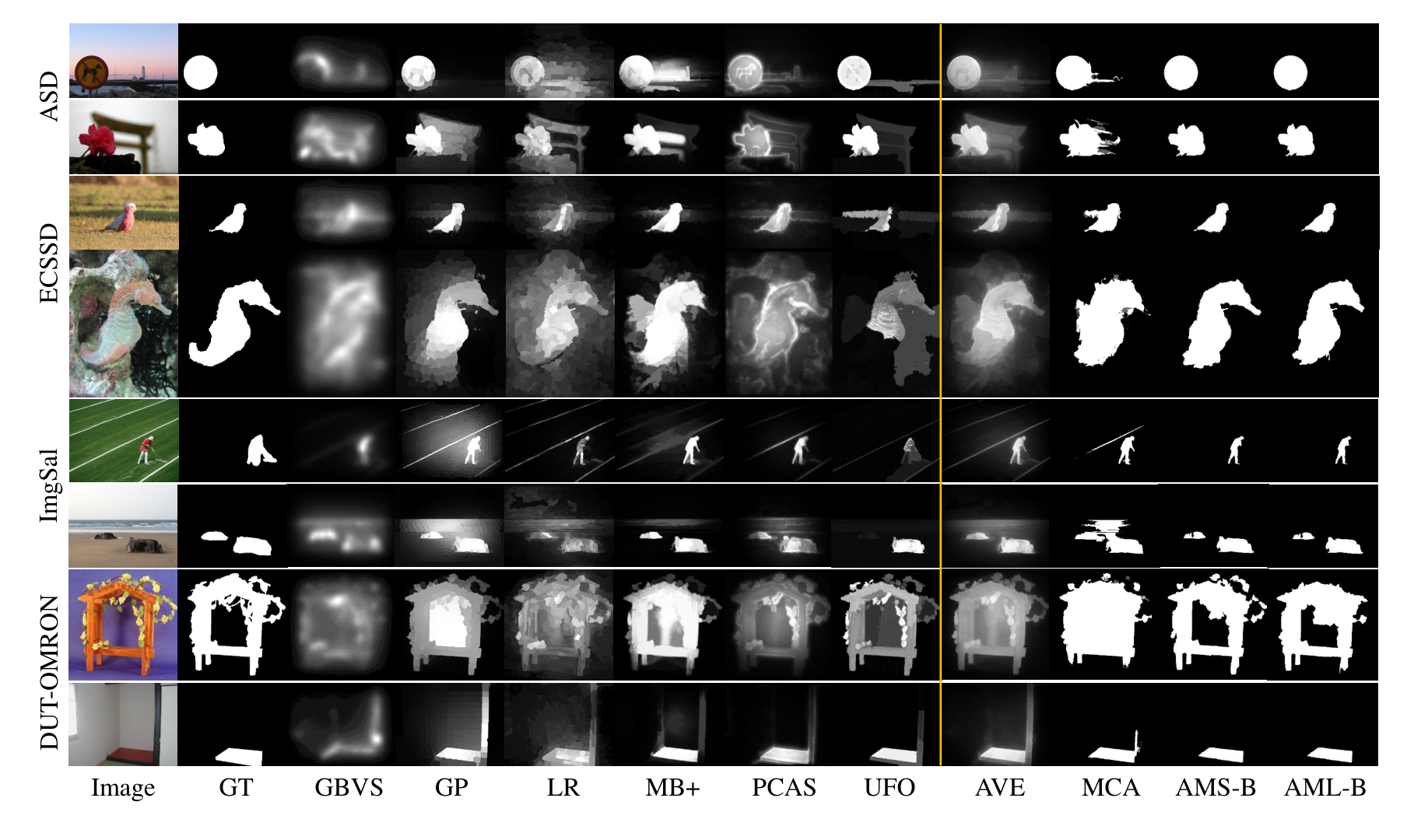
Figure 7 shows some examples of the results of candidate saliency models, the average saliency maps, MCA model and the AM model on the four datasets.

By evaluating the AM model with various combinations following four strategies, we conclude that the AM model substantially improves the performance regardless of the candidate models. In this section, we discuss the rationality of the reference map and the expertise respectively.

As mentioned in Section III, the reference map $S_{\textup{Ref}}$ is directly derived from $P(F)$ in Eq. 3, so that it should provide a natural scheme to introduce the information about salient object detection. In practice, the reference map is propagated from the consensus map of the external knowledge and the candidate saliency maps. Theoretically, the external knowledge can be any reasonable assumptions or currently existing models. In this paper, we address the inevitability of the reference map as one of the main components of the AM model. Thus, we firstly investigate the necessity of the reference map and then discuss the influences of different selections of the external knowledge.

We choose DRFI, GP, LR, MB+, TLLT and UFO as candidate saliency models and report the mean F-measure of the saliency integration results based on ECSSD dataset. As in Table V, the first row shows the performances when different external knowledge is incorporated to compute the reference map, while the second row uses the external knowledge directly as an additional candidate saliency map. Obviously, the external knowledge being incorporated into the reference map results in better integration than it being integrated as another candidate map. Even when the external knowledge is a saliency model with inferior performance, incorporating the external knowledge for the reference map results in better integration results than taking the external knowledge as another candidate saliency model (first column of Table V). Thus, introducing the external knowledge receives performance enhancement in practice.

Further, from Table II, it can be perceived that when using the same expertise estimation method, the better the quality of the reference map, the higher performance the integration can be received. Apparently, the incorporation of the reference map is critical to the performance enhancement.

As mentioned in Section III, during the CA updating process, the reference map is updated by averaging the candidate saliency maps. Thus, we conduct a small scale experiment to evaluate whether the reference map should be updated at every iteration. We test with three combinations on ECSSD dataset: 1) DHSNet, GP, IT, 2) GP, LR, PCAS, and 3) GC, GP, PCAS. By updating the reference map in each generation, the mean F-measure of the above three combinations are higher than keeping the reference map unchanged by averagely 2.01%, 0.23% and 0.06% for AMS-B, AMS-C, AMS-D and 1.30%, 0.33%, 0.07% for AML-B, AML-C, AML-D respectively. Thus, we finally decide to update the reference map by considering both the theoretical inference and the practice.

According to Table II, AML performs similarly well or slightly better than AMS in general when the same external knowledge is introduced. However, there are some exceptions. For instance, the AMS-B outperforms the AML-B by averagely 2.2% in “Deep Models Combinations”. The reason behind this is that different from the latent-variable-based expertise, the statistics-based expertise borrows information from the reference map as the approximated ‘Ground Truth’ as in Section IV-A. Thus, the accuracy of the statistics-based expertise is influenced by the quality of the reference map. In “Deep Models Combinations”, the high performances of deep candidates largely enhance the quality of the reference map, such that the AMS-B outperforms the AML-B significantly.

To quantitatively investigate the contributions of the reference map and the expertise, we also experiment each unit of the AM model on ECSSD dataset with a combination of candidate models including DRFI, GP, LR, MB+, TLLT and UFO, as shown in Table IV. The basic framework is an integration of candidate saliency models with equal expertise but without the reference map based on CA. Then we add different components to the basic framework, where the letter “L” refers to the latent-variable-based expertise, “S” means the statistics-based expertise, and “Ref-B” uses the boundary-prior-based external knowledge. From Table IV, it is obvious that the introduction of the reference map significantly enhances the performance of the basic CA framework. The involvement of the statistics-based expertise and the latent-variable-based expertise also improves the performance of the basic framework respectively. Finally, the statistics-based integration and the latent-variable-based integration with the reference map result in similarly better performances than only incorporating single unit in CA. Thus, the incorporation of both the reference map and the expertise of saliency models results in the best performance.

The proposed AM model synchronizes the $p$-th candidate by using its continuous map and the other candidates as binary maps during the CA process. Such updating form keeps the actual saliency intensity of the current candidate map and eliminates diverse semantic meanings and magnitudes from the other saliency models, as mentioned in Section IV. In Table VI, we present the mean F-measure of the integration results by using 1) only continuous maps for integration, 2) only binary maps for integration, and 3) both continuous and binary maps for integration. It can be perceived that using both the continuous maps and binary maps produces the best integration results. Although the resulted maps by using both continuous and binary maps are only slightly better than or equal to the results by using only binary maps, it does not increase the computation complexity and even reduces the numbers of thresholding process once per iteration.

As mentioned in Section II-B, the synchronizing updating rule of the cellular automaton is designed to converge the evolved cells to a stable state after several generations. We compute the absolute difference of the $S_{\textup{Ref}}^{t}$ and $S_{\textup{Ref}}^{t-1}$ in Eq. 5 at each generation, and plot the average absolute difference between $S_{\textup{Ref}}^{t}$ and $S_{\textup{Ref}}^{t-1}$ of all the superpixels on one image, with a combination of MB [46], BSCA [19], RC [14], GBVS [5], COV [29] and FT [9] on ECSSD dataset. The result is illustrated on Figure 5 (c). As is shown, the designed updating rule for cellular automaton can make the $S_{\textup{Ref}}^{t}$ rapidly converge within five iterations.

We implement our method in MATLAB R2014b using a Windows desktop with an i5-3570 CPU at 3.40GHz. The running time of AMS-B on ECSSD dataset ranges from 1.28s (2-model-combination) to 1.32s (8-model-combination) per image, while AML-B ranges from 1.38s (2-model-combination) to 2.06s (8-model-combination) in average, without code optimization. The AML and AMS show comparable performances, but AML takes longer time in running the EM algorithm.

References

- [1] E. Rahtu, J. Kannala, M. Salo, and J. Heikkilä, “Segmenting salient objects from images and videos,” in Proc. ECCV, 2010, pp. 366–379.
- [2] C. Guo and L. Zhang, “A novel multiresolution spatiotemporal saliency detection model and its applications in image and video compression,” TIP, vol. 19, no. 1, pp. 185–198, 2010.
- [3] X.-S. Hua, T. Mei, and S. Li, “When multimedia advertising meets the new internet era,” in Workshop on Multimedia Signal Processing. IEEE, 2008, pp. 1–5.
- [4] L. Itti, C. Koch, and E. Niebur, “A model of saliency-based visual attention for rapid scene analysis,” TPAMI, vol. 20, no. 11, pp. 1254–1259, 1998.
- [5] J. Harel, C. Koch, and P. Perona, “Graph-based visual saliency,” in NIPS, 2006, pp. 545–552.
- [6] D. Walther and C. Koch, “Modeling attention to salient proto-objects,” Neural Networks, vol. 19, no. 9, pp. 1395–1407, 2006.
- [7] N. Bruce and J. Tsotsos, “Saliency based on information maximization,” in NIPS, 2005, pp. 155–162.
- [8] X. Hou and L. Zhang, “Saliency detection: A spectral residual approach,” in Proc. CVPR. IEEE, 2007, pp. 1–8.
- [9] R. Achanta, S. Hemami, F. Estrada, and S. Susstrunk, “Frequency-tuned salient region detection,” in Proc. CVPR. IEEE, 2009, pp. 1597–1604.
- [10] T. Judd, K. Ehinger, F. Durand, and A. Torralba, “Learning to predict where humans look,” in Proc. ICCV. IEEE, 2009, pp. 2106–2113.
- [11] M. Jiang, J. Xu, and Q. Zhao, “Saliency in crowd,” in Proc. ECCV. Springer, 2014, pp. 17–32.
- [12] O. L. Meur, P. L. Callet, D. Barba, and D. Thoreau, “A coherent computational approach to model bottom-up visual attention,” TPAMI, vol. 28, no. 5, pp. 802–817, 2006.
- [13] L. Zhang, M. H. Tong, T. K. Marks, H. Shan, and G. W. Cottrell, “Sun: A bayesian framework for saliency using natural statistics,” Journal of Vision, vol. 8, no. 7, p. 32, 2008.
- [14] M. Cheng, N. J. Mitra, X. Huang, P. H. Torr, and S. Hu, “Global contrast based salient region detection,” TPAMI, vol. 37, no. 3, pp. 569–582, 2015.
- [15] S. Lu, V. Mahadevan, and N. Vasconcelos, “Learning optimal seeds for diffusion-based salient object detection,” in Proc. CVPR. IEEE, 2014, pp. 2790–2797.
- [16] W. Zhu, S. Liang, Y. Wei, and J. Sun, “Saliency optimization from robust background detection,” in Proc. CVPR. IEEE, 2014, pp. 2814–2821.
- [17] T. Shi, M. Liang, and X. Hu, “A reverse hierarchy model for predicting eye fixations,” in Proc. CVPR. IEEE, 2014, pp. 2822–2829.
- [18] R. Liu, J. Cao, Z. Lin, and S. Shan, “Adaptive partial differential equation learning for visual saliency detection,” in Proc. CVPR. IEEE, 2014, pp. 3866–3873.
- [19] Y. Qin, H. Lu, Y. Xu, and H. Wang, “Saliency detection via cellular automata,” in Proc. CVPR. IEEE, 2015, pp. 110–119.
- [20] N. Liu, J. Han, D. Zhang, S. Wen, and T. Liu, “Predicting eye fixations using convolutional neural networks,” in Proc. CVPR. IEEE, 2015, pp. 362–370.
- [21] R. Zhao, W. Ouyang, H. Li, and X. Wang, “Saliency detection by multi-context deep learning,” in Proc. CVPR. IEEE, 2015, pp. 1265–1274.
- [22] N. Tong, H. Lu, X. Ruan, and M.-H. Yang, “Salient object detection via bootstrap learning,” in Proc. CVPR. IEEE, 2015, pp. 1884–1892.
- [23] C. Gong, D. Tao, W. Liu, S. J. Maybank, M. Fang, K. Fu, and J. Yang, “Saliency propagation from simple to difficult,” in Proc. CVPR. IEEE, 2015, pp. 2531–2539.
- [24] D. Zhang, J. Han, C. Li, and J. Wang, “Co-saliency detection via looking deep and wide,” in Proc. CVPR. IEEE, 2015, pp. 2994–3002.
- [25] M. Feng, A. Borji, and H. Lu, “Fixation prediction with a combined model of bottom-up saliency and vanishing point,” in WACV. IEEE, 2016, pp. 1–7.
- [26] Y. Xu, X. Hong, Q. He, G. Zhao, and M. Pietikäinen, “A task-driven eye tracking dataset for visual attention analysis,” in International Conference on Advanced Concepts for Intelligent Vision Systems. Springer, 2015, pp. 637–648.
- [27] L. Wang, H. Lu, X. Ruan, and M.-H. Yang, “Deep networks for saliency detection via local estimation and global search,” in Proc. CVPR. IEEE, 2015, pp. 3183–3192.
- [28] C. Kanan, M. H. Tong, L. Zhang, and G. W. Cottrell, “Sun: Top-down saliency using natural statistics,” Visual Cognition, vol. 17, no. 6-7, pp. 979–1003, 2009.
- [29] E. Erdem and A. Erdem, “Visual saliency estimation by nonlinearly integrating features using region covariances,” Journal of Vision, vol. 13, no. 4, p. 11, 2013.
- [30] R. Margolin, A. Tal, and L. Zelnik-Manor, “What makes a patch distinct?” in Proc. CVPR. IEEE, 2013, pp. 1139–1146.
- [31] X. Hou, J. Harel, and C. Koch, “Image signature: Highlighting sparse salient regions,” TPAMI, vol. 34, no. 1, pp. 194–201, 2012.
- [32] X. Shen and Y. Wu, “A unified approach to salient object detection via low rank matrix recovery,” in Proc. CVPR. IEEE, 2012, pp. 853–860.
- [33] Y. Xu, X. Hong, X. Liu, and G. Zhao, “Saliency detection via bi-directional propagation,” Journal of Visual Communication and Image Representation, vol. 53, pp. 113–121, 2018.
- [34] C. Shen and Q. Zhao, “Webpage saliency,” in Proc. ECCV, 2014, pp. 33–46.
- [35] N. D. Bruce, C. Catton, and S. Janjic, “A deeper look at saliency: Feature contrast, semantics, and beyond,” in Proc. CVPR. IEEE, 2016, pp. 516–524.
- [36] J. Pan, K. McGuinness, E. Sayrol, N. O’Connor, and X. Giro-i Nieto, “Shallow and deep convolutional networks for saliency prediction,” in Proc. CVPR. IEEE, 2016.
- [37] O. Le Meur and Z. Liu, “Saliency aggregation: Does unity make strength?” in Proc. ACCV. Springer, 2014, pp. 18–32.
- [38] R. Song, Y. Liu, R. R. Martin, and P. L. Rosin, “Saliency-guided integration of multiple scans,” in Proc. CVPR. IEEE, 2012, pp. 1474–1481.
- [39] L. Mai, Y. Niu, and F. Liu, “Saliency aggregation: a data-driven approach,” in Proc. CVPR. IEEE, 2013, pp. 1131–1138.
- [40] J. Wang, A. Borji, C.-C. J. Kuo, and L. Itti, “Learning a combined model of visual saliency for fixation prediction,” TIP, vol. 25, no. 4, pp. 1566–1579, 2016.
- [41] A. Borji, D. N. Sihite, and L. Itti, “Salient object detection: A benchmark,” in Proc. ECCV. Springer, 2012, pp. 414–429.
- [42] L. Mai and F. Liu, “Comparing salient object detection results without ground truth,” in Proc. ECCV. Springer, 2014, pp. 76–91.
- [43] A. Borji, M.-M. Cheng, H. Jiang, and J. Li, “Salient object detection: A benchmark,” TIP, vol. 24, no. 12, pp. 5706–5722, 2015.
- [44] N. Liu and J. Han, “Dhsnet: Deep hierarchical saliency network for salient object detection,” in Proc. CVPR, 2016, pp. 678–686.
- [45] P. Jiang, N. Vasconcelos, and J. Peng, “Generic promotion of diffusion-based salient object detection,” in Proc. ICCV. IEEE, 2015, pp. 217–225.
- [46] J. Zhang, S. Sclaroff, Z. Lin, X. Shen, B. Price, and R. Mech, “Minimum barrier salient object detection at 80 fps,” in Proc. ICCV. IEEE, 2015, pp. 1404–1412.
- [47] R. Trichet and N. E. O’Connor, “A flexible ensemble-svm for computer vision tasks,” in Advanced Video and Signal Based Surveillance (AVSS). IEEE, 2016.
- [48] D. Zhang, J. Han, and Y. Zhang, “Supervision by fusion: Towards unsupervised learning of deep salient object detector,” in Proc. ICCV. IEEE, 2017, pp. 4048–4056.
- [49] R. Quan, J. Han, D. Zhang, F. Nie, X. Qian, and X. Li, “Unsupervised salient object detection via inferring from imperfect saliency models,” TMM, vol. 1, p. 1, 2017.
- [50] S. Goferman, L. Zelnik-Manor, and A. Tal, “Context-aware saliency detection,” TPAMI, vol. 34, no. 10, pp. 1915–1926, 2012.
- [51] N. Otsu, “A threshold selection method from gray-level histograms,” Automatica, vol. 11, no. 285-296, pp. 23–27, 1975.
- [52] J. Von Neumann, “The general and logical theory of automata,” Cerebral Mechanisms in Behavior, pp. 1–41, 1951.
- [53] S. Wolfram, “Statistical mechanics of cellular automata,” Reviews of Modern Physics, vol. 55, no. 3, p. 601, 1983.
- [54] Y. Qin, M. Feng, H. Lu, and G. W. Conttrell, “Hierarchical cellular automata for visual saliency,” IJCV, pp. 1–20, 2018.
- [55] Y. Wei, F. Wen, W. Zhu, and J. Sun, “Geodesic saliency using background priors,” in Proc. ECCV. Springer, 2012, pp. 29–42.
- [56] X. Li, H. Lu, L. Zhang, X. Ruan, and M.-H. Yang, “Saliency detection via dense and sparse reconstruction,” in Proc. ICCV. IEEE, 2013, pp. 2976–2983.
- [57] Q. Wang, W. Zheng, and R. Piramuthu, “Grab: Visual saliency via novel graph model and background priors,” in Proc. CVPR. IEEE, 2016, pp. 535–543.
- [58] J. Wang, H. Jiang, Z. Yuan, C. Ming-Ming, X. Hu, and N. Zheng, “Salient object detection: A discriminative regional feature integration approach,” IJCV, vol. 123, no. 2, pp. 251–268, 2017.
- [59] J. Han, D. Zhang, X. Hu, L. Guo, J. Ren, and F. Wu, “Background prior-based salient object detection via deep reconstruction residual,” TCSVT, vol. 25, no. 8, pp. 1309–1321, 2015.
- [60] D. Zhang, J. Han, L. Jiang, S. Ye, and X. Chang, “Revealing event saliency in unconstrained video collection,” TIP, vol. 26, no. 4, pp. 1746–1758, 2017.
- [61] Q. Liu, X. Hong, B. Zou, J. Chen, Z. Chen, and G. Zhao, “Hierarchical contour closure based holistic salient object detection,” TIP, 2017.
- [62] J. A. Hartigan and M. A. Wong, “Algorithm as 136: A k-means clustering algorithm,” Journal of the Royal Statistical Society. Series C (Applied Statistics), vol. 28, no. 1, pp. 100–108, 1979.
- [63] V. Gopalakrishnan, Y. Hu, and D. Rajan, “Random walks on graphs for salient object detection in images,” TIP, vol. 19, no. 12, pp. 3232–3242, 2010.
- [64] B. Jiang, L. Zhang, H. Lu, C. Yang, and M.-H. Yang, “Saliency detection via absorbing markov chain,” in Proc. ICCV. IEEE, 2013, pp. 1665–1672.
- [65] Z. Ren, Y. Hu, L.-T. Chia, and D. Rajan, “Improved saliency detection based on superpixel clustering and saliency propagation,” in Proc. Multimedia. ACM, 2010, pp. 1099–1102.
- [66] C. Yang, L. Zhang, H. Lu, X. Ruan, and M.-H. Yang, “Saliency detection via graph-based manifold ranking,” in Proc. CVPR, 2013, pp. 3166–3173.
- [67] J. Whitehill, T.-f. Wu, J. Bergsma, J. R. Movellan, and P. L. Ruvolo, “Whose vote should count more: Optimal integration of labels from labelers of unknown expertise,” in NIPS, 2009, pp. 2035–2043.
- [68] R. Mairon and O. Ben-Shahar, “A closer look at context: From coxels to the contextual emergence of object saliency,” in Proc. ECCV. Springer, 2014, pp. 708–724.
- [69] J. Shi, Q. Yan, L. Xu, and J. Jia, “Hierarchical image saliency detection on extended cssd,” TPAMI, vol. 38, no. 4, pp. 717–729, 2016.
- [70] Q. Hou, M.-M. Cheng, X.-W. Hu, A. Borji, Z. Tu, and P. Torr, “Deeply supervised salient object detection with short connections,” TPAMI, 2018.
- [71] G. Li and Y. Yu, “Deep contrast learning for salient object detection,” in Proc. CVPR. IEEE, 2016.
- [72] J. Dai, Y. Li, K. He, and J. Sun, “R-fcn: Object detection via region-based fully convolutional networks,” in NIPS, 2016, pp. 379–387.
- [73] G. Li and Y. Yu, “Visual saliency based on multiscale deep features,” in Proc. CVPR. IEEE, 2015, pp. 5455–5463.
- [74] J. Li, M. D. Levine, X. An, X. Xu, and H. He, “Visual saliency based on scale-space analysis in the frequency domain,” TPAMI, vol. 35, no. 4, pp. 996–1010, 2013.
- [75] T. Liu, Z. Yuan, J. Sun, J. Wang, N. Zheng, X. Tang, and H.-Y. Shum, “Learning to detect a salient object,” TPAMI, vol. 33, no. 2, pp. 353–367, 2011.
- [76] R. Achanta, A. Shaji, K. Smith, A. Lucchi, P. Fua, and S. Susstrunk, “Slic superpixels compared to state-of-the-art superpixel methods,” TPAMI, vol. 34, no. 11, pp. 2274–2282, 2012.
- [77] P. Krähenbühl and V. Koltun, “Efficient inference in fully connected crfs with gaussian edge potentials,” in Proc. NIPS, 2011, pp. 109–117.
- [78] D. Zhang, D. Meng, and J. Han, “Co-saliency detection via a self-paced multiple-instance learning framework,” TPAMI, vol. 39, no. 5, pp. 865–878, 2017.
- [79] X. Yao, J. Han, D. Zhang, and F. Nie, “Revisiting co-saliency detection: A novel approach based on two-stage multi-view spectral rotation co-clustering,” TIP, vol. 26, no. 7, pp. 3196–3209, 2017.
- [80] K. J. Ponti, Moacir and, M. Riva, d. T. deCampos, and C. Zor, “A decision cognizant kullback–leibler divergence,” Pattern Recognition, vol. 61, pp. 470–478, 2017.