跳到论文正文
W Papers独立论文阅读器 arXiv:1608.01400 论文正文 计算阅读时间 · 0%
引用这篇论文根据当前论文元数据生成,正式投稿前建议核对。


License: arXiv.org perpetual non-exclusive license
arXiv:1608.01400v1 [astro-ph.HE] 04 Aug 2016
\corresp

victor.ambrus@e-uvt.ro

Anderson-Witting transport coefficients for flows in general relativity

Victor E. Ambru s , Affiliation: Department of Physics, West University of Timi
s
,
oara, Bd. Vasile Pârvan 4, Timi
s
,
oara, RO 300223, Romania
Abstract

The transport coefficients induced by the Anderson-Witting approximation of the collision term in the relativistic Boltzmann equation are derived for close to equilibrium flows in general relativity. Using the tetrad formalism, it is shown that the expression for these coefficients is the same as that obtained on flat space-time, in agreement with the generalized equivalence principle.

1 INTRODUCTION

Relativistic hydrodynamics constitutes a relatively new area of research, being fundamental for the understanding of fluid flows in extreme conditions, either when the typical velocities involved approach the speed of light, or when the space-time curvature becomes significant [1]. Applications from the first category include the quark-gluon plasma [2], while from the second category, we mention astrophysical phenomena such as stellar collapse [3], accretion problems [4] or cosmology [5].

In many problems of astrophysical importance where the flow is sufficiently rarefied that the hydrodynamic (continuum) approximation cannot be applied, a kinetic theory description is required [6]. Such an approach has the advantage that the set of hydrodynamic conservation equations, which is highly non-linear in the viscous regime, emerges from the relativistic Boltzmann equation, where the advection is performed in a simple manner. In particular, for flows not far from equilibrium, the hydrodynamic limit of the Boltzmann equation can be obtained through the Chapman-Enskog expansion [7].

In this paper, we employ the Chapman-Enskog procedure to derive expressions for the transport coefficients when the Anderson-Witting approximation for the collision term in the relativistic Boltzmann equation is employed. We consider relativistic flows on an arbitrary background space-time, thus extending the results in Refs. [7, 8], obtained for the Minkowski space-time. In our analysis, we highlight a procedure for obtaining expressions for the non-equilibrium contributions to the stress-energy tensor (SET), involving the computation of a special type of moments of the equilibrium distribution function, which we summarise in the appendix. The conclusion of our study is that the expressions for the transport coefficients is identical to those obtained on the flat Minkowski space-time in Refs. [7, 8]. We also present a comparison with the results reported in Refs. [7, 9] for the Marle model.

2 ECKART AND LANDAU FRAMES

In the Eckart frame [10], the macroscopic velocity uμu^{\mu} is defined to be parallel to the particle flow four-vector NμN^{\mu}, such that:

Nμ=n​uμ,Tμ​ν=E​uμ​uν+(P+ω¯)​Δμ​ν+2​q(μCLOSE​uOPENν)+πμ​ν,N^{\mu}=nu^{\mu},\qquad T^{\mu\nu}=Eu^{\mu}u^{\nu}+(P+\overline{\omega})\Delta^{\mu\nu}+2q^{(\mu}u^{\nu)}+\pi^{\mu\nu}, (1)

such that uμ=Nμ/−Nμ​Nμu^{\mu}=N^{\mu}/\sqrt{-N_{\mu}N^{\mu}}. In the above, gμ​νg^{\mu\nu} is the space-time metric, Δμ​ν=uμ​uν+gμ​ν\Delta^{\mu\nu}=u^{\mu}u^{\nu}+g^{\mu\nu} is the projector on the hypersurface perpendicular to uμu^{\mu}, nn is the macroscopic number density, EE is the energy density, PP is the hydrostatic pressure, while the dynamic pressure ω¯\overline{\omega}, heat flux qμq^{\mu} and pressure deviator πμ​ν\pi^{\mu\nu} comprise the non-equilibrium terms.11 1 We use the signature (−,+,+,+)(-,+,+,+) for the metric and geometrical units in which c=G=1c=G=1 throughout this paper.

Once the SET and uμu^{\mu} are known, all other quantities can be obtained using:

n=−uμ​Nμ=−Nμ​Nμ,E=uμ​uν​Tμ​ν,P+ω¯=13​Δμ​ν​Tμ​ν,qμ=−Δμ​uλν​Tν​λ,πμ​ν=T<μ​ν>,n=-u_{\mu}N^{\mu}=\sqrt{-N_{\mu}N^{\mu}},\qquad E=u_{\mu}u_{\nu}T^{\mu\nu},\qquad P+\overline{\omega}=\frac{1}{3}\Delta_{\mu\nu}T^{\mu\nu},\qquad q^{\mu}=-\Delta^{\mu}{}_{\nu}u_{\lambda}T^{\nu\lambda},\qquad\pi^{\mu\nu}=T^{<\mu\nu>}, (2)

where the notation A<μ​ν>A^{<\mu\nu>} refers to:

A<μ​ν>≡[12(ΔμΔνλ+σΔμΔνσ)λ−13Δμ​νΔλ​σ]Aλ​σ.A^{<\mu\nu>}\equiv\left[\frac{1}{2}\left(\Delta^{\mu}{}_{\lambda}\Delta^{\nu}{}_{\sigma}+\Delta^{\mu}{}_{\sigma}\Delta^{\nu}{}_{\lambda}\right)-\frac{1}{3}\Delta^{\mu\nu}\Delta_{\lambda\sigma}\right]A^{\lambda\sigma}. (3)

In the Landau (energy) frame [11], the four-velocity is defined as an eigenvector of Tμ​νT^{\mu\nu}:

Tμ​uLνν=−EL​uLμ,T^{\mu}{}_{\nu}u^{\nu}_{L}=-E_{L}u^{\mu}_{L}, (4)

where the subscript LL indicates that the velocity and the energy density are expressed with respect to the Landau frame. Since ΔL;νμ​uL;λ​Tν​λ=0\Delta^{\mu}_{L;\nu}u_{L;\lambda}T^{\nu\lambda}=0, it can be seen that in this frame, the heat flux (or energy dissipation) is everywhere nil, such that NμN^{\mu} and Tμ​νT^{\mu\nu} take the following form:

Nμ=nL​uLμ+𝒥Lμ,Tμ​ν=EL​uLμ​uLν+(PL+ω¯L)​ΔLμ​ν+πLμ​ν.N^{\mu}=n_{L}u^{\mu}_{L}+\mathcal{J}^{\mu}_{L},\qquad T^{\mu\nu}=E_{L}u^{\mu}_{L}u^{\nu}_{L}+(P_{L}+\overline{\omega}_{L})\Delta_{L}^{\mu\nu}+\pi^{\mu\nu}_{L}. (5)

Thus, in the Landau frame, NμN^{\mu} and uLμu_{L}^{\mu} are no longer parallel. Close to local thermodynamic equilibrium, the quantity 𝒥Lμ\mathcal{J}^{\mu}_{L} can be linked to the heat flux of the Eckart frame via [1]:

𝒥Lμ=−nE+P​qμ.\mathcal{J}^{\mu}_{L}=-\frac{n}{E+P}q^{\mu}. (6)

If the fluid is in local thermodynamic equilibrium, the Landau and Eckart frame coincide. For small departures from equilibrium, the nonequilibrium quantities ω¯\overline{\omega}, qμq^{\mu} and πμ​ν\pi^{\mu\nu} can be written in terms of the thermodynamic forces ∇μuμ\nabla_{\mu}u^{\mu}, Δμ​ν​∇νT−uν​∇νuμ\Delta^{\mu\nu}\nabla_{\nu}T-u^{\nu}\nabla_{\nu}u^{\mu} and Δμ​ν​∇<νuμ>\Delta^{\mu\nu}\nabla_{<\nu}u_{\mu>} as follows [1, 7]:

ω¯=−η​∇μuμ,qμ=−λ⁡(Δμ​ν​∇νT+T​uν​∇νuμ),πμ​ν=−2​μ​∇<μuν>,\overline{\omega}=-\eta\nabla_{\mu}u^{\mu},\qquad q^{\mu}=-\lambda\left(\Delta^{\mu\nu}\nabla_{\nu}T+Tu^{\nu}\nabla_{\nu}u^{\mu}\right),\qquad\pi_{\mu\nu}=-2\mu\nabla_{<\mu}u_{\nu>}, (7)

which define the transport coefficients η\eta, λ\lambda and μ\mu, known as the coefficients of bulk viscosity, thermal conductivity and shear viscosity, respectively [7].

3 BOLTZMANN EQUATION IN THE ANDERSON-WITTING APPROXIMATION

The Boltzmann equation can be written in conservative form with respect to a tetrad field eα^μe_{\hat{\alpha}}^{\mu} as follows [9, 12]:

1−g​∂μ(−g​pα^​eα^μ​f)−p0^​∂∂pi^​(Γi^​pα^​pβ^p0^α^​β^​f)=J⁡[f],\frac{1}{\sqrt{-g}}\partial_{\mu}\left(\sqrt{-g}p^{\hat{\alpha}}e_{\hat{\alpha}}^{\mu}f\right)-p^{\hat{0}}\frac{\partial}{\partial p^{\hat{i}}}\left(\Gamma^{\hat{i}}{}_{{\hat{\alpha}}{\hat{\beta}}}\frac{p^{\hat{\alpha}}p^{\hat{\beta}}}{p^{\hat{0}}}f\right)=J[f], (8)

where hatted indices denote tetrad components, pα^p^{\hat{\alpha}} represent the tetrad components of the on-shell particle four-momentum vector, ff is the one-particle distribution function and J⁡[f]J[f] represents the Boltzmann collision integral. The tetrad components of the hydrodynamic variables Nα^N^{\hat{\alpha}} and Tα^​β^T^{{\hat{\alpha}}{\hat{\beta}}} can be obtained as moments of ff [7]:

Nα^=∫d3​pp0^​f​pα^,Tα^​β^=∫d3​pp0^​f​pα^​pβ^.N^{\hat{\alpha}}=\int\frac{d^{3}p}{p^{\hat{0}}}f\,p^{\hat{\alpha}},\qquad T^{{\hat{\alpha}}{\hat{\beta}}}=\int\frac{d^{3}p}{p^{\hat{0}}}f\,p^{\hat{\alpha}}p^{\hat{\beta}}. (9)

Due to the complicated nature of the collision integral, model equations for the collision term are customarily employed. Here, we consider the Anderson-Witting approximation [7, 8]:

JA−W​[f]=p⋅uLτ​(f−fL(eq)),J_{\rm A-W}[f]=\frac{p\cdot u_{L}}{\tau}(f-f^{(\mathrm{eq})}_{L}), (10)

where τ\tau is the relaxation time. The equilibrium distribution function fL(eq)f^{(\mathrm{eq})}_{L} is defined in terms of quantities expressed with respect to the Landau frame:

fL(eq)=nL4​π​m2​TL​K2​(ζL)​exp⁡(p⋅uLTL),Neq;Lα^=nL​uLα^,Teq;Lα^​β^=EL​uLα^​uLβ^+PL​ΔLα^​β^.f^{(\mathrm{eq})}_{L}=\frac{n_{L}}{4\pi m^{2}T_{L}K_{2}(\zeta_{L})}\exp\left(\frac{p\cdot u_{L}}{T_{L}}\right),\qquad N^{{\hat{\alpha}}}_{\rm eq;L}=n_{L}u^{\hat{\alpha}}_{L},\qquad T^{{\hat{\alpha}}{\hat{\beta}}}_{\rm eq;L}=E_{L}u^{\hat{\alpha}}_{L}u^{\hat{\beta}}_{L}+P_{L}\Delta^{{\hat{\alpha}}{\hat{\beta}}}_{L}. (11)

In the above, mm is the particle mass, ζL≡m/TL\zeta_{L}\equiv m/T_{L} is the relativistic coldness [1], Kn​(ζL)K_{n}(\zeta_{L}) denotes the modified Bessel functions of the third kind, PL=nL​TLP_{L}=n_{L}T_{L} is the hydrostatic pressure and the Landau energy ELE_{L} and Landau temperature TLT_{L} are linked through EL=nL​m​G​(ζL)−PLE_{L}=n_{L}mG(\zeta_{L})-P_{L}.

In Ref. [9], the transport coefficients corresponding to the Marle collision term were analysed for flows in general relativity. In this paper, we extend the results of Ref. [9] by performing a similar analysis of the transport coefficients arising in the Anderson-Witting model.

4 CHAPMAN-ENSKOG EXPANSION

In order to perform the Chapman-Enskog expansion, we consider δ​f≡f−f(eq)\delta f\equiv f-f^{(\mathrm{eq})} and τ\tau to be small. Thus, the deviation δ​f\delta f from equilibrium can be approximated by keeping only the zeroth order f=f(eq)f=f^{(\mathrm{eq})} on the left hand side in Eq. (8), such that:

δ​f=τ⁡[1−g​∂μ(−g​pα^​eα^μp⋅u​f(eq))−p0^​∂∂pi^​(Γi^​pα^​pβ^p0^​(p⋅u)α^​β^​f(eq))+(∇α^uβ^)​pα^​pβ^(p⋅u)2​f(eq)].\delta f=\tau\left[\frac{1}{\sqrt{-g}}\partial_{\mu}\left(\sqrt{-g}\frac{p^{\hat{\alpha}}e_{\hat{\alpha}}^{\mu}}{p\cdot u}f^{(\mathrm{eq})}\right)-p^{\hat{0}}\frac{\partial}{\partial p^{\hat{i}}}\left(\Gamma^{\hat{i}}{}_{{\hat{\alpha}}{\hat{\beta}}}\frac{p^{\hat{\alpha}}p^{\hat{\beta}}}{p^{\hat{0}}(p\cdot u)}f^{(\mathrm{eq})}\right)+(\nabla_{\hat{\alpha}}u_{\hat{\beta}})\frac{p^{\hat{\alpha}}p^{\hat{\beta}}}{(p\cdot u)^{2}}f^{(\mathrm{eq})}\right]. (12)

In the above, the subscript LL was dropped for quantities on the right hand side of the equation, since the Landau and the Eckart quantities coincide when f=f(eq)f=f^{(\mathrm{eq})}. We emphasize that the above equation is different from the one obtained in Ref. [8], since it is written in conservative form, such that its moments can be easily obtained. Indeed, integrating the above equation over the momentum space gives:

δ​T0α^1​…​αn=τ⁡[−∇β^T1β^​α^1​…​α^n+(∇β^uγ^)​T2β^​γ^​α^1​…​α^n],whereTnα^1​…​α^s=∫d3​pp0^​pα^1⋯pα^s(−p⋅u)n​f(eq),\delta T_{0}^{{\hat{\alpha}}_{1}\dots\alpha_{n}}=\tau\left[-\nabla_{\hat{\beta}}T_{1}^{{\hat{\beta}}{\hat{\alpha}}_{1}\dots{\hat{\alpha}}_{n}}+(\nabla_{\hat{\beta}}u_{\hat{\gamma}})T_{2}^{{\hat{\beta}}{\hat{\gamma}}{\hat{\alpha}}_{1}\dots{\hat{\alpha}}_{n}}\right],\quad{\rm where}\quad T_{n}^{{\hat{\alpha}}_{1}\dots{\hat{\alpha}}_{s}}=\int\frac{d^{3}p}{p^{\hat{0}}}\,\frac{p^{{\hat{\alpha}}_{1}}\cdots p^{{\hat{\alpha}}_{s}}}{(-p\cdot u)^{n}}f^{(\mathrm{eq})}, (13)

where the covariant derivative arises naturally due to the conservative form of Eq. (12). A comparison of the above equation with Eqs.(34) and (36) from Ref. [8] shows that, besides moments of type Tnα^1​…​α^sT^{{\hat{\alpha}}_{1}\dots{\hat{\alpha}}_{s}}_{n} with n=1n=1, the conservative approach also requires the computation of the moments with n=2n=2. We present an analysis of such moments relevant for the present work in the Appendix.

4.1 The coefficient of bulk viscosity η\eta

Taking the trace of Eq. (5) shows that δTα^α^=3ω¯L\delta T^{\hat{\alpha}}{}_{\hat{\alpha}}=3\overline{\omega}_{L}, since Teq;α^α^=−EL+3​PLT^{\hat{\alpha}}_{{\rm eq};{\hat{\alpha}}}=-E_{L}+3P_{L}. Furthermore, the definition (13) and the properties (34) can be used to show that δTα^α^=−m2δT0\delta T^{\hat{\alpha}}{}_{\hat{\alpha}}=-m^{2}\delta T_{0}. Setting n=0n=0 in Eq. (13) gives:

ω¯=−τ​m23​[−∇γ^T1γ^+(∇γ^uρ^)​T2γ^​ρ^].\overline{\omega}=-\frac{\tau m^{2}}{3}\left[-\nabla_{\hat{\gamma}}T_{1}^{\hat{\gamma}}+(\nabla_{\hat{\gamma}}u_{\hat{\rho}})T_{2}^{{\hat{\gamma}}{\hat{\rho}}}\right]. (14)

The divergence of T1γ^=T110​uγ^T_{1}^{\hat{\gamma}}=T_{11}^{0}u^{\hat{\gamma}} can be computed by substituting T110T_{11}^{0} from Eq. (32):

∇γ^T1γ^=T110​∇γ^uγ^+D​T110=−Pm2​(1−3cv)​∇γ^uγ^,\nabla_{\hat{\gamma}}T^{\hat{\gamma}}_{1}=T_{11}^{0}\nabla_{\hat{\gamma}}u^{\hat{\gamma}}+DT_{11}^{0}=-\frac{P}{m^{2}}\left(1-\frac{3}{c_{v}}\right)\nabla_{\hat{\gamma}}u^{\hat{\gamma}}, (15)

where the notation D=uγ^​∇γ^D=u^{\hat{\gamma}}\nabla_{\hat{\gamma}} was used. In the Chapman-Enskog procedure, the derivatives DD are replaced by making use of the conservation equations at the Euler level [1, 9]:

D​n=−n​∇γ^uγ^,D​E=−(E+P)​∇γ^uγ^,D​T=−Tcv​∇γ^uγ^,D​uα^=−1E+P​Δα^​γ^​∇γ^P,Dn=-n\nabla_{\hat{\gamma}}u^{\hat{\gamma}},\qquad DE=-(E+P)\nabla_{\hat{\gamma}}u^{\hat{\gamma}},\qquad DT=-\frac{T}{c_{v}}\nabla_{\hat{\gamma}}u^{\hat{\gamma}},\qquad Du^{\hat{\alpha}}=-\frac{1}{E+P}\Delta^{{\hat{\alpha}}{\hat{\gamma}}}\nabla_{\hat{\gamma}}P, (16)

where the specific heat cvc_{v} is given by:

cv=ζ2+5​G​ζ−G2​ζ2−1.c_{v}=\zeta^{2}+5G\zeta-G^{2}\zeta^{2}-1. (17)

In the above, G≡G⁡(ζ)=K3​(ζ)/K2​(ζ)G\equiv G(\zeta)=K_{3}(\zeta)/K_{2}(\zeta). Using Eqs. (30) and Eq. (33) for T2γ^​ρ^T^{{\hat{\gamma}}{\hat{\rho}}}_{2}, together with the property uρ^​∇γ^uρ^=0u^{\hat{\rho}}\nabla_{\hat{\gamma}}u_{\hat{\rho}}=0, it can be shown that substituting Eq. (15) into Eq. (14) allows η\eta to be put in the following form:

η=τ​P​(−1−1cv+ζ​G3−ζ29+ζ2​Ki29​K2),\eta=\tau P\left(-1-\frac{1}{c_{v}}+\frac{\zeta G}{3}-\frac{\zeta^{2}}{9}+\frac{\zeta^{2}{\rm Ki}_{2}}{9K_{2}}\right), (18)

where Ki2≡Ki2​(ζ){\rm Ki}_{2}\equiv{\rm Ki}_{2}(\zeta) is defined in the Appendix. It can be checked that the above result coincides with those obtained in Refs. [7, 8] on flat space-time by using the following relation:

Ki2​(ζ)=ζ⁡[−Ki1​(ζ)+K1​(ζ)].{\rm Ki}_{2}(\zeta)=\zeta[-{\rm Ki}_{1}(\zeta)+K_{1}(\zeta)]. (19)

4.2 Coefficient of thermal conductivity λ\lambda

In flows close to equilibrium, δ​Nα^=−nP+E​qα^\delta N^{\hat{\alpha}}=-\frac{n}{P+E}q^{\hat{\alpha}}, by virtue of Eqs. (5) and (6), since Neqα^=nL​uLα^N^{\hat{\alpha}}_{\rm eq}=n_{L}u^{\hat{\alpha}}_{L}. Setting n=1n=1 in Eq. (13) allows the heat flux to be written as:

qα^=−τ⁡(P+E)n​[−∇β^T1α^​β^+(∇β^uγ^)​T2α^​β^​γ^]=τ⁡(P+E)n​[n​D​uα^+Δα^​β^​∇β^T121],q^{\hat{\alpha}}=-\frac{\tau(P+E)}{n}\left[-\nabla_{\hat{\beta}}T^{{\hat{\alpha}}{\hat{\beta}}}_{1}+(\nabla_{\hat{\beta}}u_{\hat{\gamma}})T^{{\hat{\alpha}}{\hat{\beta}}{\hat{\gamma}}}_{2}\right]=\frac{\tau(P+E)}{n}\left[nDu^{\hat{\alpha}}+\Delta^{{\hat{\alpha}}{\hat{\beta}}}\nabla_{\hat{\beta}}T^{1}_{12}\right], (20)

where the second equality can be obtained by using the property Δα^​qβ^β^\Delta^{\hat{\alpha}}{}_{\hat{\beta}}q^{\hat{\beta}}= qα^q^{\hat{\alpha}}. The derivative of T121T_{12}^{1} can be obtained from Eqs. (30) and (32):

∇β^T121=13​m​[5​ζ−ζ2​G​(ζ)+ζ2​Ki1​(ζ)K2​(ζ)]​∇β^P+P3​m2​[3​ζ2−5​ζ3​G​(ζ)+ζ4​G2​(ζ)−ζ4​G​(ζ)​Ki1​(ζ)K2​(ζ)]​∇β^T.\nabla_{\hat{\beta}}T^{1}_{12}=\frac{1}{3m}\left[5\zeta-\zeta^{2}G(\zeta)+\frac{\zeta^{2}{\rm Ki}_{1}(\zeta)}{K_{2}(\zeta)}\right]\nabla_{\hat{\beta}}P+\frac{P}{3m^{2}}\left[3\zeta^{2}-5\zeta^{3}G(\zeta)+\zeta^{4}G^{2}(\zeta)-\frac{\zeta^{4}G(\zeta){\rm Ki}_{1}(\zeta)}{K_{2}(\zeta)}\right]\nabla_{\hat{\beta}}T. (21)

Using Eq. (16) to replace D​uα^Du^{\hat{\alpha}} in the expression for qα^q^{\hat{\alpha}} in Eq. (7), as well as in Eq. (20), it can be shown that the thermal conductivity is given by:

λ=τ​P​ζ4​G​(ζ)3​m​[G⁡(ζ)​Ki1​(ζ)K2​(ζ)−G2​(ζ)+5​G​(ζ)ζ−3ζ2].\lambda=\tau P\frac{\zeta^{4}G(\zeta)}{3m}\left[\frac{G(\zeta){\rm Ki}_{1}(\zeta)}{K_{2}(\zeta)}-G^{2}(\zeta)+\frac{5G(\zeta)}{\zeta}-\frac{3}{\zeta^{2}}\right]. (22)

This result is in agreement with the one reported in Refs. [7, 8].

4.3 Coefficient of shear viscosity μ\mu

Finally, μ\mu can be obtained from the expression for πα^​β^\pi^{{\hat{\alpha}}{\hat{\beta}}} by using Eq. (7). By noting that δ​T0α^​β^=ω¯​Δα^​β^+πα^​β^\delta T^{{\hat{\alpha}}{\hat{\beta}}}_{0}=\overline{\omega}\Delta^{{\hat{\alpha}}{\hat{\beta}}}+\pi^{{\hat{\alpha}}{\hat{\beta}}}, it can be shown that:

πα^​β^=η​Δα^​β^​∇γ^uγ^+τ⁡[−∇γ^T1α^​β^​γ^+(∇γ^uρ^)​T2α^​β^​γ^​ρ^].\pi^{{\hat{\alpha}}{\hat{\beta}}}=\eta\Delta^{{\hat{\alpha}}{\hat{\beta}}}\nabla_{\hat{\gamma}}u^{\hat{\gamma}}+\tau\left[-\nabla_{\hat{\gamma}}T^{{\hat{\alpha}}{\hat{\beta}}{\hat{\gamma}}}_{1}+(\nabla_{\hat{\gamma}}u_{\hat{\rho}})T^{{\hat{\alpha}}{\hat{\beta}}{\hat{\gamma}}{\hat{\rho}}}_{2}\right]. (23)

Using Eqs. (30) and (32) for T1α^​β^​γ^T^{{\hat{\alpha}}{\hat{\beta}}{\hat{\gamma}}}_{1}, the following result can be obtained:

∇γ^T1α^​β^​γ^=n​T​∇γ^uγ^​[(53−1cv)​Δα^​β^−ηα^​β^]+n​T​D​(uα^​uβ^)+2​n​T​∇<α^uβ^>.\nabla_{\hat{\gamma}}T^{{\hat{\alpha}}{\hat{\beta}}{\hat{\gamma}}}_{1}=nT\nabla_{\hat{\gamma}}u^{\hat{\gamma}}\left[\left(\frac{5}{3}-\frac{1}{c_{v}}\right)\Delta^{{\hat{\alpha}}{\hat{\beta}}}-\eta^{{\hat{\alpha}}{\hat{\beta}}}\right]+nTD(u^{\hat{\alpha}}u^{\hat{\beta}})+2nT\nabla^{<{\hat{\alpha}}}u^{{\hat{\beta}}>}. (24)

By susbtituting the above result in Eq. (23) and using Eqs. (30) and (33) for Tα^​β^​γ^​ρ^T^{{\hat{\alpha}}{\hat{\beta}}{\hat{\gamma}}{\hat{\rho}}}, πα^​β^\pi^{{\hat{\alpha}}{\hat{\beta}}} can be written as:

πα^​β^=τ​n​T​[Δα^​β^​∇γ^uγ^​(ητ​n​T+5​T2413​n​T−73+1cv)+2​(T241n​T−2)​∇<α^uβ^>].\pi^{{\hat{\alpha}}{\hat{\beta}}}=\tau nT\left[\Delta^{{\hat{\alpha}}{\hat{\beta}}}\nabla_{\hat{\gamma}}u^{\hat{\gamma}}\left(\frac{\eta}{\tau nT}+\frac{5T_{24}^{1}}{3nT}-\frac{7}{3}+\frac{1}{c_{v}}\right)+2\left(\frac{T_{24}^{1}}{nT}-2\right)\nabla^{<{\hat{\alpha}}}u^{{\hat{\beta}}>}\right]. (25)

Using the expression (18) obtained for η\eta, it can be shown that the coefficient of ∇γ^uγ^\nabla_{\hat{\gamma}}u^{\hat{\gamma}} vanishes, such that:

μ=35​(η+τ​n​T​1+cvcv)=τ​n​T15​ζ​(3​G​(ζ)−ζ+ζ​Ki2​(ζ)K2​(ζ)).\mu=\frac{3}{5}\left(\eta+\tau nT\frac{1+c_{v}}{c_{v}}\right)=\frac{\tau nT}{15}\zeta\left(3G(\zeta)-\zeta+\frac{\zeta{\rm Ki}_{2}(\zeta)}{K_{2}(\zeta)}\right). (26)

Employing Eq. (19) shows that Eq. (26) reduces to the result in Refs. [7, 8].

4.4 Analysis of the results and comparison to the Marle model

Refer to caption Refer to caption
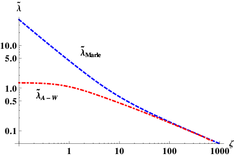
Figure 1: Comparison of the (a) shear viscosity, (b) thermal conductivity and (c) bulk viscosity coefficients obtained when the Anderson-Witting and Marle approximations for the collision term are employed. (d) The curves corresponding to ηM\eta_{\rm M} and ηA−W\eta_{\rm A-W} are almost overlapped after the scaling in Eq. (29).

In this section, the transport coefficients obtained here for the Anderson-Witting model are compared to those obtained using the Marle model when the relaxation time is set to [7, 9]:

τ=1n​σ​⟨v⟩,⟨v⟩=ζEK1​(ζE)​[e−ζE​1+ζEζE2−Γ⁡(0,ζE)],\tau=\frac{1}{n\sigma\braket{v}},\qquad\braket{v}=\frac{\zeta_{E}}{K_{1}(\zeta_{E})}\left[e^{-\zeta_{E}}\frac{1+\zeta_{E}}{\zeta_{E}^{2}}-\Gamma(0,\zeta_{E})\right], (27)

where σ\sigma is the differential cross section and Γ⁡(ν,z)\Gamma(\nu,z) is the incomplete Gamma function [13]. In order to perform the comparison, “effective” transport coefficients may be defined, such that they only depend on ζ=m/T\zeta=m/T [9]:

η~=σ​ηm,λ~=σ​λ,μ~=σ​μm.\widetilde{\eta}=\frac{\sigma\eta}{m},\qquad\widetilde{\lambda}=\sigma\lambda,\qquad\widetilde{\mu}=\frac{\sigma\mu}{m}. (28)

The log-log plots in Fig. 1(a) and (b) show that the behaviour of μ~\widetilde{\mu} and λ~\widetilde{\lambda} in the non-relativistic (large ζ\zeta) limit is the same in the Marle and Anderson-Witting models. However, as ζ→0\zeta\rightarrow 0, the effective heat conductivity λ~A−W\widetilde{\lambda}_{\rm A-W} in the Anderson-Witting model tends to 4/34/3, while in the Marle model, λ~M→∞\widetilde{\lambda}_{\rm M}\rightarrow\infty. Even though not visible in the plot, λ~A−W\widetilde{\lambda}_{\rm A-W} has a point of local maximum at ζ=0.023151\zeta=0.023151, where its value differs only slightly from its value at ζ=0\zeta=0 (λ~max=1.33348\widetilde{\lambda}_{\rm max}=1.33348). In the case of the coefficient of bulk viscosity, Fig. 1(c) shows that it exhibits the same main features in both models, namely: it decreases to 00 as ζ→0\zeta\rightarrow 0 and ζ→∞\zeta\rightarrow\infty and it attains a maximum value at a finite value of ζ\zeta. While in the Marle model, the maximum is attained at ζmax;M=1.535\zeta_{\rm max;M}=1.535, where η~M​(ζmax;M)=0.0044664\widetilde{\eta}_{M}(\zeta_{\rm max;M})=0.0044664, in the A-W model, ζmax;A−W=2.23578\zeta_{\rm max;A-W}=2.23578 and η~M​(ζmax;M)=0.00166279\widetilde{\eta}_{M}(\zeta_{\rm max;M})=0.00166279. It is surprising to note that the bulk viscosity in the two models are almost exactly related through a scaling of the argument and overall value such that their point of maximum coincides, i.e.:

η~M​(ζ/ζmax;M)η~M​(ζmax;M)≃η~A−W​(ζ/ζmax;A−W)η~A−W​(ζmax;A−W).\frac{\widetilde{\eta}_{\rm M}\left(\zeta/\zeta_{\rm max;M}\right)}{\widetilde{\eta}_{\rm M}(\zeta_{\rm max;M})}\simeq\frac{\widetilde{\eta}_{\rm A-W}\left(\zeta/\zeta_{\rm max;A-W}\right)}{\widetilde{\eta}_{\rm A-W}(\zeta_{\rm max;A-W})}. (29)

Fgure 1(d) shows a comparison between the two sides of the above equation.

5 CONCLUSION

In this paper, we employed the conservative form of the Boltzmann equation based on the tetrad formalism to obtain expressions for the transport coefficients corresponding to the Anderson-Witting model for reltivistic flows in general relativity. Our conclusion is that the form of these coefficients coincides with that obtained in flat space-time, in agreement with the equilvalence principle. Further, a graphical analysis showed that an appropriate scaling brings the coefficient of bulk viscosity η\eta in the Anderson-Witting to a form which is very close to that in the Marle model.

6 ACKNOWLEDGMENTS

This work was supported by a grant of the Romanian National Authority for Scientific Research and Innovation, CNCS-UEFISCDI, project number PN-II-RU-TE-2014-4-2910.

Appendix A APPENDIX

In this section, the moments of f(eq)f^{(\mathrm{eq})} defined in Eq. (13) are computed for n=0,1,2n=0,1,2 with ss ranging from 00 up to 22, 33 and 44, respectively. In order to compute these moments, the following notation is employed:

Tn=Tn​00,Tnα^=Tn​10​uα^,Tnα^​β^=Tn​20​uα^​uβ^+Tn​21​ηα^​β^,Tnα^​β^​γ^=Tn​30​uα^​uβ^​uγ^+Tn​31​uρ^​Δα^​β^​γ^​ρ^,\displaystyle T_{n}=T_{n0}^{0},\qquad T_{n}^{{\hat{\alpha}}}=T_{n1}^{0}u^{\hat{\alpha}},\qquad T_{n}^{{\hat{\alpha}}{\hat{\beta}}}=T_{n2}^{0}u^{\hat{\alpha}}u^{\hat{\beta}}+T_{n2}^{1}\eta^{{\hat{\alpha}}{\hat{\beta}}},\qquad T_{n}^{{\hat{\alpha}}{\hat{\beta}}{\hat{\gamma}}}=T_{n3}^{0}u^{\hat{\alpha}}u^{\hat{\beta}}u^{\hat{\gamma}}+T_{n3}^{1}u_{\hat{\rho}}\Delta^{{\hat{\alpha}}{\hat{\beta}}{\hat{\gamma}}{\hat{\rho}}},
Tnα^​β^​γ^​ρ^=Tn​40​uα^​uβ^​uγ^​uρ^+Tn​41​(uα^​uβ^​ηγ^​ρ^+uα^​uγ^​ηβ^​ρ^+uα^​uρ^​ηβ^​γ^+uβ^​uγ^​ηα^​ρ^+uβ^​uρ^​ηα^​γ^+uγ^​uρ^​ηα^​β^)+Tn​42​Δα^​β^​γ^​ρ^,\displaystyle T_{n}^{{\hat{\alpha}}{\hat{\beta}}{\hat{\gamma}}{\hat{\rho}}}=T_{n4}^{0}u^{\hat{\alpha}}u^{\hat{\beta}}u^{\hat{\gamma}}u^{\hat{\rho}}+T_{n4}^{1}(u^{\hat{\alpha}}u^{\hat{\beta}}\eta^{{\hat{\gamma}}{\hat{\rho}}}+u^{\hat{\alpha}}u^{\hat{\gamma}}\eta^{{\hat{\beta}}{\hat{\rho}}}+u^{\hat{\alpha}}u^{\hat{\rho}}\eta^{{\hat{\beta}}{\hat{\gamma}}}+u^{\hat{\beta}}u^{\hat{\gamma}}\eta^{{\hat{\alpha}}{\hat{\rho}}}+u^{\hat{\beta}}u^{\hat{\rho}}\eta^{{\hat{\alpha}}{\hat{\gamma}}}+u^{\hat{\gamma}}u^{\hat{\rho}}\eta^{{\hat{\alpha}}{\hat{\beta}}})+T_{n4}^{2}\Delta^{{\hat{\alpha}}{\hat{\beta}}{\hat{\gamma}}{\hat{\rho}}}, (30)

where Δα^​β^​γ^​ρ^=ηα^​β^​ηγ^​ρ^+ηα^​γ^​ηβ^​ρ^+ηα^​ρ^​ηβ^​γ^\Delta^{{\hat{\alpha}}{\hat{\beta}}{\hat{\gamma}}{\hat{\rho}}}=\eta^{{\hat{\alpha}}{\hat{\beta}}}\eta^{{\hat{\gamma}}{\hat{\rho}}}+\eta^{{\hat{\alpha}}{\hat{\gamma}}}\eta^{{\hat{\beta}}{\hat{\rho}}}+\eta^{{\hat{\alpha}}{\hat{\rho}}}\eta^{{\hat{\beta}}{\hat{\gamma}}}. Finding analytic expressions for the coefficients Tn​spT_{ns}^{p} defined in Eqs. (30) makes the subject of the present section.

For the case n=0n=0, the relevant coefficients for the moments up to s≤2s\leq 2 are:

T000=nm​(G−4ζ),T010=n,T020=n​m​G,T021=n​mζ,T_{00}^{0}=\frac{n}{m}\left(G-\frac{4}{\zeta}\right),\qquad T_{01}^{0}=n,\qquad T_{02}^{0}=nmG,\qquad T_{02}^{1}=\frac{nm}{\zeta}, (31)

where G≡G⁡(ζ)=K3​(ζ)/K2​(ζ)G\equiv G(\zeta)=K_{3}(\zeta)/K_{2}(\zeta).

The relevant coefficients for the case when n=1n=1 are:

T100=nm2​(ζ​G−4−ζ​Ki1K2),T110=nm​(G−4ζ),T120=n3​(8−ζ​G+ζ​Ki1K2),\displaystyle T_{10}^{0}=\frac{n}{m^{2}}\left(\zeta G-4-\frac{\zeta{\rm Ki}_{1}}{K_{2}}\right),\qquad T_{11}^{0}=\frac{n}{m}\left(G-\frac{4}{\zeta}\right),\qquad T_{12}^{0}=\frac{n}{3}\left(8-\zeta G+\frac{\zeta{\rm Ki}_{1}}{K_{2}}\right),
T121=n3​(5−ζ​G+ζ​Ki1K2),T130=n​m​(G+2ζ),T131=n​mζ,\displaystyle T_{12}^{1}=\frac{n}{3}\left(5-\zeta G+\frac{\zeta{\rm Ki}_{1}}{K_{2}}\right),\qquad T_{13}^{0}=nm\left(G+\frac{2}{\zeta}\right),\qquad T_{13}^{1}=\frac{nm}{\zeta}, (32)

where it is understood that the argument of GG and of all modified Bessel functions is ζ\zeta, while Kin≡Kin​(ζ)=∫0∞d​t​(cosh⁡t)−n​e−ζ​cosh⁡t{\rm Ki}_{n}\equiv{\rm Ki}_{n}(\zeta)=\int_{0}^{\infty}dt\,(\cosh t)^{-n}e^{-\zeta\cosh t} denotes the integral of the modified Bessel functions [7]. The results in Eq. (32) for T120T_{12}^{0}, T121T_{12}^{1}, T130T_{13}^{0} and T131T_{13}^{1} are in exact agreement with those reported in Eqs. (44)-(47) of Ref. [8].

Finally, the coefficients for the case when n=2n=2 are given by:

T200=nm3​(ζ+8ζ−2​G−ζ​Ki2K2),T210=T100,T220=n3​m​(6​G−24ζ−ζ+ζ​Ki2K2),\displaystyle T_{20}^{0}=\frac{n}{m^{3}}\left(\zeta+\frac{8}{\zeta}-2G-\frac{\zeta{\rm Ki}_{2}}{K_{2}}\right),\qquad T_{21}^{0}=T_{10}^{0},\qquad T_{22}^{0}=\frac{n}{3m}\left(6G-\frac{24}{\zeta}-\zeta+\frac{\zeta{\rm Ki}_{2}}{K_{2}}\right),\quad
T221=n3​m​(3​G−12ζ−ζ+ζ​Ki2K2),T230=n⁡(6−ζ​G+ζ​Ki1K2),T231=T121,\displaystyle T_{22}^{1}=\frac{n}{3m}\left(3G-\frac{12}{\zeta}-\zeta+\frac{\zeta{\rm Ki}_{2}}{K_{2}}\right),\qquad T_{23}^{0}=n\left(6-\zeta G+\frac{\zeta{\rm Ki}_{1}}{K_{2}}\right),\qquad T_{23}^{1}=T_{12}^{1},\qquad\quad
T240=n​m5​(2​G+40ζ+ζ−ζ​Ki2K2),T241=n​m15​(−3​G+30ζ+ζ−ζ​Ki2K2),T242=T241+n​T.\displaystyle T_{24}^{0}=\frac{nm}{5}\left(2G+\frac{40}{\zeta}+\zeta-\frac{\zeta{\rm Ki}_{2}}{K_{2}}\right),\qquad T_{24}^{1}=\frac{nm}{15}\left(-3G+\frac{30}{\zeta}+\zeta-\frac{\zeta{\rm Ki}_{2}}{K_{2}}\right),\qquad T_{24}^{2}=T_{24}^{1}+nT. (33)

As before, all functions depend on ζ\zeta, unless otherwise indicated.

Before ending this Appendix, it is worth mentioning that the moments Tnα^1​…​α^sT^{{\hat{\alpha}}_{1}\dots{\hat{\alpha}}_{s}}_{n} satisfy the following relations:

−uα^s​Tnα^1​…​α^s=Tn−1α^1​…​α^s−1,−ηα^s−1​α^s​Tnα^1​…​α^s=m2​Tnα^1​…​α^s−2.-u_{{\hat{\alpha}}_{s}}T_{n}^{{\hat{\alpha}}_{1}\dots{\hat{\alpha}}_{s}}=T_{n-1}^{{\hat{\alpha}}_{1}\dots{\hat{\alpha}}_{s-1}},\qquad-\eta_{{\hat{\alpha}}_{s-1}{\hat{\alpha}}_{s}}T_{n}^{{\hat{\alpha}}_{1}\dots{\hat{\alpha}}_{s}}=m^{2}T_{n}^{{\hat{\alpha}}_{1}\dots{\hat{\alpha}}_{s-2}}. (34)

References

  • [1] L. Rezzolla and O. Zanotti, Relativistic hydrodynamics (Oxford University Press, Oxford, UK, 2013).
  • [2] B. V. Jacak and B. Muller, Science 337, 310–314 (2012).
  • [3] C. L. Fryer, Stellar Collapse (Kluwer Academic Publishers, Dordrecht, Netherlands, 2004).
  • [4] F. Banyuls, J. A. Font, J. M. Ibanez, J. M. Marti, and J. A. Miralles, Astrophys. J. 476, 221–231 (1997).
  • [5] G. F. R. Ellis, R. Maartens, and M. A. H. MacCallum, Relativistic cosmology (Cambridge University Press, Cambridge, UK, 2012).
  • [6] T. Tsumura, T. Kunihiro, and K. Ohnishi, Phys. Lett. B 646, 134–140 (2007).
  • [7] C. Cercignani and G. M. Kremer, The relativistic Boltzmann equation: theory and applications (Birkhäuser Verlag, Basel, Switzerland, 2002).
  • [8] J. L. Anderson and H. R. Witting, Physica 74, p. 466 (1974).
  • [9] V. E. Ambruş and I. I. Cotăescu, arXiv:1605.07043 [hep-th] (2016).
  • [10] C. Eckart, Phys. Rev. 58, 919–924 (1940).
  • [11] L. D. Landau and E. M. Lifshitz, Fluid mechanics (Pergamon Press, Oxford, UK, 1987).
  • [12] C. Y. Cardall, E. Endeve, and A. Mezzacappa, Phys. Rev. D 88, p. 023011 (2013).
  • [13] F. W. J. Olver, D. W. Lozier, R. F. Boisvert, and C. W. Clark, NIST handbook of mathematical functions (Cambridge University Press, New York, USA, 2010).