跳到论文正文
W Papers独立论文阅读器 arXiv:1608.01236 论文正文 计算阅读时间 · 0%
引用这篇论文根据当前论文元数据生成,正式投稿前建议核对。


License: arXiv.org perpetual non-exclusive license
arXiv:1608.01236v2 [math.SP] 23 Jul 2018

Sharp Poincaré inequalities in a class of non-convex sets

B. Brandolini†- F. Chiacchio† - E. B. Dryden‡ - J. J. Langford‡
Abstract.

Let γ\gamma be a smooth, non-closed, simple curve whose image is symmetric with respect to the yy-axis, and let DD be a planar domain consisting of the points on one side of γ\gamma, within a suitable distance δ\delta of γ\gamma. Denote by μ1o​d​d​(D)\mu_{1}^{odd}(D) the smallest nontrivial Neumann eigenvalue having a corresponding eigenfunction that is odd with respect to the yy-axis. If γ\gamma satisfies some simple geometric conditions, then μ1o​d​d​(D)\mu_{1}^{odd}(D) can be sharply estimated from below in terms of the length of γ\gamma, its curvature, and δ\delta. Moreover, we give explicit conditions on δ\delta that ensure μ1o​d​d​(D)=μ1​(D)\mu_{1}^{odd}(D)=\mu_{1}(D). Finally, we can extend our bound on μ1o​d​d​(D)\mu_{1}^{odd}(D) to a certain class of three-dimensional domains. In both the two- and three-dimensional settings, our domains are generically non-convex.

Key words and phrases: 
Neumann eigenvalues; lower bounds; non-convex domains
2010 Mathematics Subject Classification
35J25,35P15

† Dipartimento di Matematica e Applicazioni “R. Caccioppoli”

Università degli Studi di Napoli Federico II

Monte S. Angelo, via Cintia, I-80126 Napoli, Italy

brandolini@unina.it

francesco.chiacchio@unina.it

‡ Department of Mathematics, Bucknell University

One Dent Drive, Lewisburg, PA 17837, USA

emily.dryden@bucknell.edu

jeffrey.langford@bucknell.edu

1. Introduction

Let D⊂ℝnD\subset\mathbb{R}^{n} be a bounded, connected, Lipschitz domain. We study the classical free membrane problem in DD, that is,

(1.1) {−Δ​u=μ​uin​D∂u∂𝐧=0on​∂D,\left\{\begin{array}[]{ll}-\Delta u=\mu u&\mbox{in}\>D\\ \\ \frac{\partial u}{\partial\mathbf{n}}=0&\mbox{on}\>\partial D,\end{array}\right.

where 𝐧\mathbf{n} denotes the exterior unit normal to ∂D\partial D. We arrange the eigenvalues of (1.1) in a non-decreasing sequence {μn​(D)}n∈ℕ0\{\mu_{n}(D)\}_{n\in\mathbb{N}_{0}}, where each eigenvalue is repeated according to its multiplicity. The first eigenfunction of (1.1) is clearly a constant with eigenvalue μ0​(D)=0\mu_{0}(D)=0 for any DD. We shall be interested in the first non-trivial eigenvalue μ1​(D)\mu_{1}(D), which admits the following variational characterization:

μ1(D)=min{∫D|∇ψ|2​𝑑x​𝑑y∫Dψ2​𝑑x​𝑑y:ψ∈H1(D)∖{0},∫Dψdxdy=0},\mu_{1}(D)=\min\left\{\frac{\displaystyle\int_{D}|\nabla\psi|^{2}dxdy}{\displaystyle\int_{D}\psi^{2}dxdy}:\>\psi\in H^{1}(D)\setminus\{0\},\>\int_{D}\psi dxdy=0\right\},

where H1​(D)H^{1}(D) is the usual Sobolev space of square-integrable functions with weak first-order partials that are also square-integrable; all functions considered here and in what follows are real-valued.

As is well known, many difficulties arise in estimating μ1​(D)\mu_{1}(D). One reason for this is the lack of monotonicity of eigenvalues with respect to set inclusion. Another is the fact that eigenfunctions corresponding to μ1​(D)\mu_{1}(D) must change sign, and localizing the nodal line seems to be a hard problem (e.g., [15]).

Despite these difficulties, there are lower bounds on μ1​(D)\mu_{1}(D) in certain situations. The celebrated Payne-Weinberger [19] inequality states that if DD is a convex domain with diameter d⁡(D)d(D), then

(1.2) μ1​(D)≥π2d​(D)2.\mu_{1}(D)\geq\frac{\pi^{2}}{d(D)^{2}}.

The above estimate is asymptotically sharp, since μ1​(D)​d​(D)2\mu_{1}(D)d(D)^{2} tends to π2\pi^{2} for a parallelepiped all but one of whose dimensions shrink to 0. Estimate (1.2) fails for general non-convex sets, as can be seen by considering a domain consisting of two identical squares connected by a thin corridor. Such a counterexample suggests that a lower bound on μ1​(D)\mu_{1}(D) for non-convex domains should involve geometric quantities other than the diameter. In [5, 7] such a lower bound involves the isoperimetric constant relative to DD, and in [13] a lower bound is given in terms of an LαL^{\alpha} norm of the Riemann conformal mapping of the unit disk onto DD. Thus the problem of finding a lower bound on μ1​(D)\mu_{1}(D) for non-convex domains is often shifted to another geometric problem. Related and further results may be found, for instance, in [6, 8, 10, 11, 12, 20].

We consider a class of domains that have a line or plane of symmetry, but that are typically non-convex. Letting μ1o​d​d\mu_{1}^{odd} denote the smallest nontrivial Neumann eigenvalue having a corresponding eigenfunction that is odd with respect to this line or plane, we give explicit lower bounds on μ1o​d​d\mu_{1}^{odd}. In the two-dimensional case, we let γ⁡(s)=(x⁡(s),y⁡(s)),s∈[0,L],\gamma(s)=(x(s),y(s)),\>s\in[0,L], be a smooth, non-closed, simple curve, parametrized with respect to its arc length, and whose image is symmetric with respect to the yy-axis. That is,

x⁡(L−s)=−x⁡(s),y⁡(L−s)=y⁡(s),s∈[0,L2].x(L-s)=-x(s),\hskip 8.50012pty(L-s)=y(s),\hskip 8.50012pts\in\left[0,\frac{L}{2}\right].

Consider the domain DD consisting of the points on one side of γ\gamma, within a suitable distance δ\delta of γ\gamma. Using the normal vector to γ⁡(s)\gamma(s) obtained by rotating γ′​(s)\gamma^{\prime}(s) clockwise by π2\frac{\pi}{2}, we may describe DD as follows (see Figure 1):

(1.3) D={(x(s)+ry′(s),y(s)−rx′(s)):s∈(0,L),r∈(0,δ)}.D=\left\{(x(s)+ry^{\prime}(s),y(s)-rx^{\prime}(s)):\>s\in(0,L),\>r\in(0,\delta)\right\}.
Figure 1. A typical domain DD described in the Fermi coordinate system.

Denote by μ1o​d​d\mu_{1}^{odd} the smallest nontrivial Neumann eigenvalue having a corresponding eigenfunction that is odd with respect to the yy-axis. Our main result is

Theorem 1.1.

Suppose that the curvature k⁡(s)k(s) of γ\gamma is concave in [0,L][0,L] and let δ>0\delta>0 be such that 1+δ​k​(s)>01+\delta k(s)>0 in [0,L][0,L]. If DD is simply connected, then

μ1o​d​d​(D)≥B​π2L2,\mu_{1}^{odd}(D)\geq B\frac{\pi^{2}}{L^{2}},

where B=minr∈[0,δ],s∈[0,L]⁡1(1+r​k​(s))2B=\displaystyle{\min_{r\in\left[0,\delta\right],\,s\in\left[0,L\right]}}\frac{1}{(1+rk(s))^{2}}; equality holds if γ\gamma is a line segment.

Thus we give a sharp lower bound on μ1o​d​d\mu_{1}^{odd} that is reminiscent of the bound in [19], with a correction factor that encodes the relevant geometry of our domains. We stress that this result falls in the category of lower bounds obtained in [19, 5, 7, 13], since under certain explicit assumptions on LL and δ\delta, we show that μ1​(D)\mu_{1}(D) coincides with μ1o​d​d​(D)\mu_{1}^{odd}(D) (see Propositions 3.1 and 3.2). Roughly speaking, this phenomenon occurs whenever δ\delta is sufficiently smaller than LL. If such a relationship does not hold, Theorem 1.1 is still relevant, as μ1o​d​d​(D)\mu_{1}^{odd}(D) can be realized as the lowest eigenvalue of the Laplacian with mixed boundary conditions on D+={(x,y)∈D:x>0}D^{+}=\{(x,y)\in D:x>0\}. Sharp bounds for such eigenvalues have been obtained in [1] (see also [2, §2.5] and [18]). Finally, we are able to adapt the argument used to prove Theorem 1.1 to give the same lower bound on μ1o​d​d\mu_{1}^{odd} for certain three-dimensional domains that are not necessarily convex.

The paper is organized as follows. In §2, we prove Theorem 1.1. In §3, we give conditions under which μ1o​d​d​(D)\mu_{1}^{odd}(D) coincides with μ1​(D)\mu_{1}(D), as well as examples illustrating our two-dimensional results. We extend our two-dimensional results to certain three-dimensional domains in §4, and conclude with an appendix that details some of the computations associated with the Fermi coordinate system that we use in our proofs.

2. Proof of the main result

The focus of this section will be the proof of Theorem 1.1. We will introduce a Fermi coordinate system on DD and slice DD into thin pieces, with the mean value of an odd eigenfunction vanishing on each slice. Since the slices are thin, we are close to being in a one-dimensional setting and the following lemma from [19, §2] will play a key role.

Lemma 2.1.

Let p⁡(s)p(s) be a concave, non-negative function on the interval [0,L][0,L]. Then for any piecewise twice differentiable function v⁡(s)v(s) that satisfies

∫0Lv⁡(s)​p​(s)​𝑑s=0,\int_{0}^{L}v(s)p(s)ds=0,

it follows that

∫0L(v′​(s))2​p​(s)​𝑑s≥π2L2​∫0Lv​(s)2​p​(s)​𝑑s.\int_{0}^{L}(v^{\prime}(s))^{2}p(s)ds\geq\frac{\pi^{2}}{L^{2}}\int_{0}^{L}v(s)^{2}p(s)ds.
Remark 2.1.

Suppose pp is also even with respect to L2\frac{L}{2}, and v⁡(s)v(s) is a sufficiently smooth function satisfying v⁡(L2)=0v\left(\dfrac{L}{2}\right)=0. Define a new function w⁡(s)w(s) that is equal to v⁡(s)v(s) on [0,L2][0,\frac{L}{2}], and is equal to the odd reflection of v⁡(s)v(s) in the line s=L2s=\frac{L}{2} on [L2,L][\frac{L}{2},L]. Then Lemma 2.1 applies to w⁡(s)w(s) and a straightforward computation shows that

∫0L2(w′​(s))2​p​(s)​𝑑s≥π2L2​∫0L2w​(s)2​p​(s)​𝑑s.\int_{0}^{\frac{L}{2}}(w^{\prime}(s))^{2}p(s)ds\geq\frac{\pi^{2}}{L^{2}}\int_{0}^{\frac{L}{2}}w(s)^{2}p(s)ds.

Since w⁡(s)=v⁡(s)w(s)=v(s) on [0,L2][0,\frac{L}{2}], we may replace ww by vv in the preceding inequality. We will use this observation in our proof of Proposition 3.2.

We are now ready to prove Theorem 1.1.

Proof of Theorem 1.1.

Fix n∈ℕn\in\mathbb{N}. Let us denote by distγ(x,y)\mathop{\mathrm{dist}}\nolimits_{\gamma}(x,y) the distance of a generic point (x,y)∈D(x,y)\in D to γ\gamma and, for any i=0,…,n−1i=0,\dots,n-1, by

Di={(x,y)∈D:i​δn<distγ(x,y)<(i+1)​δn}.D_{i}=\left\{(x,y)\in D:\>\frac{i\,\delta}{n}<\mathop{\mathrm{dist}}\nolimits_{\gamma}(x,y)<\frac{(i+1)\,\delta}{n}\right\}.

Let uu be an odd eigenfunction corresponding to μ1o​d​d​(D)\mu_{1}^{odd}(D) (from now on, for the sake of brevity, we will omit “with respect to the yy-axis”). Using the definition of eigenfunction and a Green’s formula, we see that

μ1o​d​d​(D)=∫D|∇u|2​𝑑x​𝑑y∫Du2​𝑑x​𝑑y;\mu_{1}^{odd}(D)=\frac{\displaystyle\int_{D}|\nabla u|^{2}dxdy}{\displaystyle\int_{D}u^{2}dxdy};

moreover, the fact that uu is odd implies

∫Diu​𝑑x​𝑑y=0​for all ​i=0,…,n−1.\int_{D_{i}}u\,dxdy=0\hskip 8.50012pt\text{for all }i=0,\dots,n-1.

We want to evaluate the energy of uu in any DiD_{i}. We construct a Fermi coordinate system (r,s)(r,s) whereby points (x,y)(x,y) in DD are determined by specifying the distance r=distγ(x,y)r=\mathop{\mathrm{dist}}\nolimits_{\gamma}(x,y) to the curve γ\gamma, and the arc length ss of the point on γ\gamma nearest to (x,y)(x,y). Alternatively, we observe that the co-area formula on the level sets of the distance to γ\gamma yields the same results. Changing from rectangular to Fermi coordinates (see the Appendix for details), we have

∫Di|∇u|2​𝑑x​𝑑y\displaystyle\int_{D_{i}}|\nabla u|^{2}dxdy =\displaystyle= ∫0L(∫i​δn(i+1)​δn(11+r​k​(s)​us2​(r,s)+(1+r​k​(s))​ur2​(r,s))​𝑑r)​𝑑s\displaystyle\int_{0}^{L}\left(\int_{\frac{i\,\delta}{n}}^{\frac{(i+1)\,\delta}{n}}\left(\frac{1}{1+rk(s)}u_{s}^{2}(r,s)+(1+rk(s))u_{r}^{2}(r,s)\right)dr\right)ds
≥\displaystyle\geq mins∈[0,L],r∈[i​δn,(i+1)​δn]⁡1(1+r​k​(s))2​∫0L(∫i​δn(i+1)​δnus2​(r,s)​(1+r​k​(s))​𝑑r)​𝑑s\displaystyle\min_{s\in[0,L],\,r\in\left[\frac{i\,\delta}{n},\frac{(i+1)\,\delta}{n}\right]}\frac{1}{(1+rk(s))^{2}}\int_{0}^{L}\left(\int_{\frac{i\,\delta}{n}}^{\frac{(i+1)\,\delta}{n}}u_{s}^{2}(r,s)(1+rk(s))\,dr\right)ds
≥\displaystyle\geq B​∫0L(∫i​δn(i+1)​δnus2​(r,s)​(1+r​k​(s))​𝑑r)​𝑑s,\displaystyle B\int_{0}^{L}\left(\int_{\frac{i\,\delta}{n}}^{\frac{(i+1)\,\delta}{n}}u_{s}^{2}(r,s)(1+rk(s))\,dr\right)ds,

where the first inequality follows from the hypothesis that 1+δ​k​(s)>01+\delta k(s)>0 in [0,L][0,L], and the second from the definition of BB. Let us write

∫0L(∫i​δn(i+1)​δnus2​(r,s)​(1+r​k​(s))​𝑑r)​𝑑s=I1+I2,\int_{0}^{L}\left(\int_{\frac{i\,\delta}{n}}^{\frac{(i+1)\,\delta}{n}}u_{s}^{2}(r,s)(1+rk(s))\,dr\right)ds=I_{1}+I_{2},

where

I1=∫0L(∫i​δn(i+1)​δn(us2​(r,s)−us2​(i​δn,s))​(1+r​k​(s))​𝑑r)​𝑑sI_{1}=\int_{0}^{L}\left(\int_{\frac{i\,\delta}{n}}^{\frac{(i+1)\,\delta}{n}}\left(u_{s}^{2}(r,s)-u_{s}^{2}\left(\frac{i\,\delta}{n},s\right)\right)(1+rk(s))dr\right)ds

and

I2=∫0L(∫i​δn(i+1)​δnus2​(i​δn,s)​(1+r​k​(s))​𝑑r)​𝑑s=δn​∫0Lus2​(i​δn,s)​(1+1+2​i2​δn​k​(s))​𝑑s.I_{2}=\int_{0}^{L}\left(\int_{\frac{i\,\delta}{n}}^{\frac{(i+1)\,\delta}{n}}u_{s}^{2}\left(\frac{i\,\delta}{n},s\right)(1+rk(s))dr\right)ds=\frac{\delta}{n}\int_{0}^{L}u_{s}^{2}\left(\frac{i\,\delta}{n},s\right)\left(1+\frac{1+2i}{2}\frac{\delta}{n}k(s)\right)ds.

Let AA be a common bound for the absolute value of each of uu and its first and second derivatives when expressed in Fermi coordinates. Applying the Mean Value Theorem, we deduce that

(2.1) |I1|≤2​A2​δn​|Di|.|I_{1}|\leq\frac{2A^{2}\delta}{n}|D_{i}|.

We will return to I2I_{2} in a moment; first, we note that the arguments used above may be applied to show that

∫Diu2​𝑑x​𝑑y=∫0L(∫i​δn(i+1)​δnu2​(r,s)​(1+r​k​(s))​𝑑r)​𝑑s=J1+J2,\int_{D_{i}}u^{2}dxdy=\int_{0}^{L}\left(\int_{\frac{i\,\delta}{n}}^{\frac{(i+1)\,\delta}{n}}u^{2}(r,s)(1+rk(s))\,dr\right)ds=J_{1}+J_{2},

where

J1=∫0L(∫i​δn(i+1)​δn(u2​(r,s)−u2​(i​δn,s))​(1+r​k​(s))​𝑑r)​𝑑s,J_{1}=\int_{0}^{L}\left(\int_{\frac{i\,\delta}{n}}^{\frac{(i+1)\,\delta}{n}}\left(u^{2}(r,s)-u^{2}\left(\frac{i\,\delta}{n},s\right)\right)(1+rk(s))dr\right)ds,
J2=∫0L(∫i​δn(i+1)​δnu2​(i​δn,s)​(1+r​k​(s))​𝑑r)​𝑑s=δn​∫0Lu2​(i​δn,s)​(1+1+2​i2​δn​k​(s))​𝑑s,J_{2}=\int_{0}^{L}\left(\int_{\frac{i\,\delta}{n}}^{\frac{(i+1)\,\delta}{n}}u^{2}\left(\frac{i\,\delta}{n},s\right)(1+rk(s))dr\right)ds=\frac{\delta}{n}\int_{0}^{L}u^{2}\left(\frac{i\,\delta}{n},s\right)\left(1+\frac{1+2i}{2}\frac{\delta}{n}k(s)\right)ds,

and

|J1|≤2​A2​δn​|Di|.|J_{1}|\leq\frac{2A^{2}\delta}{n}|D_{i}|.

We will next relate I2I_{2} and J2J_{2} via Lemma 2.1. Using the expression for signed curvature that may be found in the Appendix, it is straightforward to show that k⁡(s)k(s) is even with respect to L2\frac{L}{2}. Since uu is odd with respect to L2\frac{L}{2}, we have that

∫0Lu⁡(i​δn,s)​(1+1+2​i2​δn​k​(s))​𝑑s=0.\int_{0}^{L}u\left(\frac{i\,\delta}{n},s\right)\left(1+\frac{1+2i}{2}\frac{\delta}{n}k(s)\right)ds=0.

Our hypothesis that 1+δ​k​(s)>01+\delta k(s)>0 for ss in [0,L][0,L] implies that 1+1+2​i2​δn​k​(s)>01+\frac{1+2i}{2}\frac{\delta}{n}k(s)>0. Since we have also assumed that k⁡(s)k(s) is concave in [0,L][0,L], Lemma 2.1 implies that

(2.2) I2≥π2L2​J2.I_{2}\geq\frac{\pi^{2}}{L^{2}}J_{2}.

We now combine the above estimates. We have

∫Di|∇u|2​𝑑x​𝑑y\displaystyle\int_{D_{i}}|\nabla u|^{2}dxdy ≥\displaystyle\geq B⁡(I1+I2)\displaystyle B\left(I_{1}+I_{2}\right)
≥\displaystyle\geq B​δn​(∫0Lus2​(i​δn,s)​(1+1+2​i2​δn​k​(s))​𝑑s−2​A2​|Di|)\displaystyle B\frac{\delta}{n}\left(\int_{0}^{L}u_{s}^{2}\left(\frac{i\,\delta}{n},s\right)\left(1+\frac{1+2i}{2}\frac{\delta}{n}k(s)\right)ds-2A^{2}|D_{i}|\right)
≥\displaystyle\geq B​δn​(π2L2​∫0Lu2​(i​δn,s)​(1+1+2​i2​δn​k​(s))​𝑑s−2​A2​|Di|),\displaystyle B\frac{\delta}{n}\left(\frac{\pi^{2}}{L^{2}}\int_{0}^{L}u^{2}\left(\frac{i\,\delta}{n},s\right)\left(1+\frac{1+2i}{2}\frac{\delta}{n}k(s)\right)ds-2A^{2}|D_{i}|\right),

where we used (2.1) and (2.2), respectively. Using an equivalent expression for J2J_{2}, converting back to rectangular coordinates, and subtracting a positive term, we conclude that

∫Di|∇u|2​𝑑x​𝑑y≥B​π2L2​(∫Diu2​𝑑x​𝑑y−2​A2​δn​|Di|)−B​2​A2​δn​|Di|.\int_{D_{i}}|\nabla u|^{2}dxdy\geq B\frac{\pi^{2}}{L^{2}}\left(\int_{D_{i}}u^{2}\,dxdy-\frac{2A^{2}\delta}{n}|D_{i}|\right)-B\frac{2A^{2}\delta}{n}|D_{i}|.

Summing over ii, we obtain

∫D|∇u|2​𝑑x​𝑑y≥B​π2L2​∫Du2​𝑑x​𝑑y−C​δn​|D|,\int_{D}|\nabla u|^{2}dxdy\geq B\frac{\pi^{2}}{L^{2}}\int_{D}u^{2}dxdy-\frac{C\delta}{n}|D|,

with C>0C>0. Taking the limit as nn goes to +∞+\infty yields the claim.

Finally, to establish the case of equality, we take γ⁡(s)=(L2−s,0)\gamma(s)=\left(\dfrac{L}{2}-s,0\right) with s∈[0,L]s\in[0,L] so that D=(−L2,L2)×(0,δ)D=\left(-\dfrac{L}{2},\dfrac{L}{2}\right)\times(0,\delta). In this case, μ1o​d​d​(D)=π2L2\mu_{1}^{odd}(D)=\dfrac{\pi^{2}}{L^{2}}. ∎

Remark 2.2.

If γ\gamma is a curve as in Theorem 1.1, but is closed, it follows from the Four Vertex Theorem that γ\gamma is a circle and DD is an annulus; the eigenvalues of such domains may be found exactly from equations that involve cross products of derivatives of Bessel functions.

Remark 2.3.

If γ\gamma is part of the boundary of a convex domain TT, so that k⁡(s)≥0k(s)\geq 0 in [0,L][0,L], then 1+δ​k​(s)1+\delta k(s) is clearly positive for any choice of δ>0\delta>0. Thus one may remove the restriction on the value of δ\delta from Theorem 1.1 for such a γ\gamma.

Some concrete examples to which Theorem 1.1 applies will be provided at the end of §3.

3. A sufficient condition for μ1​(D)=μ1o​d​d​(D)\mu_{1}(D)=\mu_{1}^{odd}(D)

In this section we give some geometric conditions to ensure that μ1​(D)\mu_{1}(D) coincides with μ1o​d​d​(D)\mu_{1}^{odd}(D). Arguments of a similar flavor have been used in [3, 15].

Proposition 3.1.

Let γ\gamma and DD be as in Theorem 1.1 and suppose that γ\gamma may be realized as the graph of a function. We denote by Πx​(D)=(−P,P)\Pi_{x}(D)=(-P,P) the projection of DD onto the xx-axis. Let SxS_{x} denote the vertical cross sections of DD, i.e., Sx={(x~,y~)∈D:x~=x}S_{x}=\left\{(\widetilde{x},\widetilde{y})\in D:\widetilde{x}=x\right\}, and define S=maxx∈[0,P)⁡|Sx|S=\max\limits_{x\in\left[0,P\right)}\left|S_{x}\right|. If

(3.1) S2<P2​∫Dsin2⁡(π2​P​x)​𝑑x​𝑑y∫Dcos2⁡(π2​P​x)​𝑑x​𝑑y,S^{2}<P^{2}\frac{\displaystyle\int_{D}\sin^{2}\left(\frac{\pi}{2P}x\right)dxdy}{\displaystyle\int_{D}\cos^{2}\left(\frac{\pi}{2P}x\right)dxdy},

then

μ1​(D)=μ1o​d​d​(D).\mu_{1}(D)=\mu_{1}^{odd}(D).
Proof.

Suppose for the sake of reaching a contradiction that there is no odd eigenfunction corresponding to μ1​(D)\mu_{1}(D). Therefore if v⁡(x,y)v(x,y) is any eigenfunction corresponding to μ1​(D)\mu_{1}(D), then u⁡(x,y)=v⁡(x,y)+v⁡(−x,y)u(x,y)=v(x,y)+v(-x,y) is an eigenfunction that is even.

We begin by showing that the curve γδ\gamma^{\delta} parallel to γ\gamma at distance δ\delta must also be the graph of a function. Note that γ⁡(s)\gamma(s) restricted to either [0,L2]\left[0,\dfrac{L}{2}\right] or [L2,L]\left[\dfrac{L}{2},L\right] lies in the first quadrant; we assume that [0,L2]\left[0,\dfrac{L}{2}\right] is the relevant interval. Thus γ⁡(s)\gamma(s), for 0≤s≤L20\leq s\leq\dfrac{L}{2}, is the graph of a function in the first quadrant and may be parametrized by ψ⁡(t)=(T−t,f⁡(T−t))\psi(t)=(T-t,f(T-t)) for 0≤t≤T0\leq t\leq T and some function ff. Our parametrization is constructed so that we traverse γ\gamma with its original orientation. The curve

γδ​(s)=(x⁡(s)+δ​y′​(s),y⁡(s)−δ​x′​(s)), for ​0≤s≤L2,\gamma^{\delta}(s)=(x(s)+\delta y^{\prime}(s),y(s)-\delta x^{\prime}(s)),\text{ for }0\leq s\leq\frac{L}{2},

may then be parametrized by

ψδ​(t)=(T−t−δ​f′​(T−t)1+(f′​(T−t))2,f⁡(T−t)+δ​11+(f′​(T−t))2), 0≤t≤T,\psi^{\delta}(t)=\left(T-t-\delta\frac{f^{\prime}(T-t)}{\sqrt{1+(f^{\prime}(T-t))^{2}}}\,,f(T-t)+\delta\frac{1}{\sqrt{1+(f^{\prime}(T-t))^{2}}}\right),\ \ 0\leq t\leq T,

where, as we did for γδ​(s)\gamma^{\delta}(s), we are again translating along a normal vector obtained by rotating our original tangent vector clockwise by π2\dfrac{\pi}{2}. Taking the derivative with respect to tt of the first coordinate of ψδ​(t)\psi^{\delta}(t), we find that it equals −1−δ​k​(t)-1-\delta k(t), where k⁡(t)k(t) is the signed curvature of ψ⁡(t)\psi(t). However, we parametrized ψ⁡(t)\psi(t) so that it would have the same orientation as γ⁡(s)\gamma(s), so our assumption that 1+δ​k​(s)>01+\delta k(s)>0 implies that 1+δ​k​(t)>01+\delta k(t)>0. Hence the first coordinate of ψδ​(t)\psi^{\delta}(t) is strictly decreasing, and we deduce that ψδ​(t)\psi^{\delta}(t) is also the graph of a function.

Next we use nodal considerations to restrict our attention to a subset of DD. As is well-known (e.g., [9]), the nodal line u=0u=0 is a smooth curve; moreover, it cannot enclose any subdomain of DD. Our assumption that uu is even implies that the nodal domains corresponding to uu are symmetric with respect to the yy-axis, and Courant’s theorem implies that there are exactly two such nodal domains. Thus the nodal line intersects ∂D\partial D in exactly two symmetric points and it crosses the yy-axis at precisely one point inside DD. Let Πx({u=0})=[−Z,Z]\Pi_{x}(\{u=0\})=[-Z,Z] be the projection of the nodal line onto the xx-axis. Since the nodal line is a smooth curve, we see that each vertical line x=cx=c, where −Z≤c≤Z-Z\leq c\leq Z, intersects the nodal line. Let

D+={(x,y)∈D:u⁡(x,y)>0}​ and ​D−={(x,y)∈D:u⁡(x,y)<0}.D_{+}=\left\{(x,y)\in D:u(x,y)>0\right\}\text{ and }D_{-}=\left\{(x,y)\in D:u(x,y)<0\right\}.

We claim that the projection of at least one of D+D_{+} and D−D_{-} onto the xx-axis is contained in [−Z,Z][-Z,Z]. If this were not the case, we could find points (x1,y1)∈D+(x_{1},y_{1})\in D_{+} and (x2,y2)∈D−(x_{2},y_{2})\in D_{-} with |x1|,|x2|>Z|x_{1}|,|x_{2}|>Z. Since uu is even, we may assume that x1,x2>Zx_{1},x_{2}>Z. We claim that we may connect (x1,y1)(x_{1},y_{1}) to (x2,y2)(x_{2},y_{2}) via a path whose xx-coordinate is always strictly larger than ZZ. Define

γr​(s)=(x⁡(s)+r​y′​(s),y⁡(s)−r​x′​(s)), for ​0≤s≤L2​ and ​0≤r≤δ.\gamma^{r}(s)=(x(s)+ry^{\prime}(s),y(s)-rx^{\prime}(s)),\text{ for }0\leq s\leq\frac{L}{2}\text{ and }0\leq r\leq\delta.

Note that, for i=1,2i=1,2, we have (xi,yi)=γri​(si)(x_{i},y_{i})=\gamma^{r_{i}}(s_{i}) for some ri∈[0,δ]r_{i}\in[0,\delta] and some si∈[0,L2]s_{i}\in[0,\dfrac{L}{2}]. Fixing ss and letting rr vary between 00 and δ\delta, we see that γr​(s)\gamma^{r}(s) traces out a line segment. Thus we may travel along such line segments from γri​(si)\gamma^{r_{i}}(s_{i}) to either γ⁡(si)\gamma(s_{i}) or γδ​(si)\gamma^{\delta}(s_{i}) for i=1,2i=1,2 in such a way that the xx-coordinate remains strictly greater than ZZ. Our path from γr1​(s1)\gamma^{r_{1}}(s_{1}) to γr2​(s2)\gamma^{r_{2}}(s_{2}) is then completed by traveling appropriately along the boundary; we know that the boundary portion of our path has xx-coordinate strictly greater than ZZ because γ\gamma and γδ\gamma^{\delta} are both graphs of functions, and γr​(0)\gamma^{r}(0) is a line segment. By the Intermediate Value Theorem, the nodal line intersects this path, which is a contradiction. Thus the projection of at least one of D+D_{+} and D−D_{-} onto the xx-axis is contained in [−Z,Z][-Z,Z]; replacing uu with −u-u as needed, we may assume that the projection of D+D_{+} is contained in [−Z,Z][-Z,Z].

We will now use D+D_{+} to find a lower bound on μ1​(D)\mu_{1}(D). We have

(3.2) μ1​(D)=∫D+|∇u|2​𝑑x​𝑑y∫D+u2​𝑑x​𝑑y≥∫D+uy2​𝑑x​𝑑y∫D+u2​𝑑x​𝑑y=∫Πx​(D+)(∫Sx∩D+uy2​𝑑y)​𝑑x∫D+u2​𝑑x​𝑑y.\mu_{1}(D)=\frac{\displaystyle\int_{D_{+}}\left|\nabla u\right|^{2}dxdy}{\displaystyle\int_{D_{+}}u^{2}dxdy}\geq\frac{\displaystyle\int_{D_{+}}u_{y}^{2}\,dxdy}{\displaystyle\int_{D_{+}}u^{2}dxdy}=\frac{\displaystyle\int_{\Pi_{x}(D_{+})}\left(\displaystyle\int_{S_{x}\cap D_{+}}u_{y}^{2}\,dy\right)dx}{\displaystyle\int_{D_{+}}u^{2}dxdy}.

For almost every xx we have

Sx∩D+=⋃j=1∞Ijx,S_{x}\cap D_{+}=\bigcup_{j=1}^{\infty}I_{j}^{x},

where for any jj, IjxI_{j}^{x} is an open interval such that uu vanishes at one or both endpoints of IjxI_{j}^{x}. The boundary condition is potentially unknown at one of the endpoints of IjxI_{j}^{x}, but we may take an odd reflection of uu in the Dirichlet end of IjxI_{j}^{x}. Thus uu has mean value equal to zero on the doubled IjxI_{j}^{x}, and we have

∫Ixjuy2​𝑑y≥π24​|Ixj|2​∫Ixju2​𝑑y≥π24​S2​∫Ixju2​𝑑y.\int_{I_{x}^{j}}u_{y}^{2}\,dy\geq\frac{\pi^{2}}{4|I_{x}^{j}|^{2}}\int_{I_{x}^{j}}u^{2}dy\geq\frac{\pi^{2}}{4S^{2}}\int_{I_{x}^{j}}u^{2}dy.

This last consideration, together with (3.2), yields

μ1​(D)≥π24​S2.\mu_{1}(D)\geq\frac{\pi^{2}}{4S^{2}}.

On the other hand, choosing sin⁡(π2​P​x)\sin\left(\frac{\pi}{2P}x\right) as a test function for μ1​(D)\mu_{1}(D) we obtain

μ1​(D)≤π24​P2​∫Dcos2⁡(π2​P​x)​𝑑x​𝑑y∫Dsin2⁡(π2​P​x)​𝑑x​𝑑y;\mu_{1}(D)\leq\frac{\pi^{2}}{4P^{2}}\frac{\displaystyle\int_{D}\cos^{2}\left(\frac{\pi}{2P}x\right)dxdy}{\displaystyle\int_{D}\sin^{2}\left(\frac{\pi}{2P}x\right)dxdy};

combining these two inequalities on μ1​(D)\mu_{1}(D), we see that we have a contradiction to our hypothesis (3.1). ∎

Remark 3.1.

Proposition 3.1 can be stated in different ways depending on the choice of the test function used to obtain the upper bound for μ1​(D)\mu_{1}(D). A rough estimate can be obtained by choosing xx as a test function. In this case condition (3.1) becomes

S2<π24​∫Dx2​𝑑x​𝑑y|D|.S^{2}<\frac{\pi^{2}}{4}\dfrac{\displaystyle\int_{D}x^{2}dxdy}{\left|D\right|}.

Since our domain DD has a special shape, we can alternatively use cos⁡(πL​s)\cos\left(\frac{\pi}{L}s\right) as a test function in the Rayleigh quotient written in Fermi coordinates and (3.1) becomes

(3.3) S2<L24​∫0L(∫0δcos2⁡(πL​s)​(1+r​k​(s))​𝑑r)​𝑑s∫0L(∫0δsin2⁡(πL​s)​11+r​k​(s)​𝑑r)​𝑑s.S^{2}<\frac{L^{2}}{4}\frac{\displaystyle\int_{0}^{L}\left(\displaystyle\int_{0}^{\delta}\cos^{2}\left(\frac{\pi}{L}s\right)(1+rk(s))dr\right)ds}{\displaystyle\int_{0}^{L}\left(\displaystyle\int_{0}^{\delta}\sin^{2}\left(\frac{\pi}{L}s\right)\frac{1}{1+rk(s)}dr\right)ds}.

In the next proposition we show that, if γ\gamma is not the graph of a one-dimensional function, it is still possible to give a condition ensuring that μ1​(D)=μ1o​d​d​(D)\mu_{1}(D)=\mu_{1}^{odd}(D).

Proposition 3.2.

Let γ\gamma and DD be as in Theorem 1.1. Then

μ1​(D)=μ1o​d​d​(D)\mu_{1}(D)=\mu_{1}^{odd}(D)

if one of the following alternatives holds:

  1. (1)

    k⁡(s)≥0k(s)\geq 0 for all s∈[0,L]s\in[0,L] and

    (3.4) maxs∈[0,L]​δ2​(2+δ​k​(s))2<L2π2​∫0L(∫0δcos2⁡(πL​s)​(1+r​k​(s))​𝑑r)​𝑑s∫0L(∫0δsin2⁡(πL​s)​11+r​k​(s)​𝑑r)​𝑑s;\underset{s\in[0,L]}{\max}\delta^{2}(2+\delta k(s))^{2}<\dfrac{L^{2}}{\pi^{2}}\>\frac{\displaystyle\int_{0}^{L}\left(\displaystyle\int_{0}^{\delta}\cos^{2}\left(\frac{\pi}{L}s\right)(1+rk(s))dr\right)ds}{\displaystyle\int_{0}^{L}\left(\displaystyle\int_{0}^{\delta}\sin^{2}\left(\frac{\pi}{L}s\right)\frac{1}{1+rk(s)}dr\right)ds};
  2. (2)

    k⁡(s)<0k(s)<0 for all s∈[0,L]s\in[0,L] and

    (3.5) maxs∈[0,L]​4​δ2(1+δ​k​(s))2<L2π2​∫0L(∫0δcos2⁡(πL​s)​(1+r​k​(s))​𝑑r)​𝑑s∫0L(∫0δsin2⁡(πL​s)​11+r​k​(s)​𝑑r)​𝑑s;o​r\underset{s\in[0,L]}{\max}\dfrac{4\delta^{2}}{(1+\delta k(s))^{2}}<\dfrac{L^{2}}{\pi^{2}}\>\frac{\displaystyle\int_{0}^{L}\left(\displaystyle\int_{0}^{\delta}\cos^{2}\left(\frac{\pi}{L}s\right)(1+rk(s))dr\right)ds}{\displaystyle\int_{0}^{L}\left(\displaystyle\int_{0}^{\delta}\sin^{2}\left(\frac{\pi}{L}s\right)\frac{1}{1+rk(s)}dr\right)ds};or
  3. (3)

    k⁡(s)k(s) changes its sign in [0,L][0,L], and

    (3.6) max⁡{maxs∈[0,L]​δ2​(2+δ​k​(s))2,maxs∈[0,L]​4​δ2(1+δ​k​(s))2}<L2π2​∫0L(∫0δcos2⁡(πL​s)​(1+r​k​(s))​𝑑r)​𝑑s∫0L(∫0δsin2⁡(πL​s)​11+r​k​(s)​𝑑r)​𝑑s.\max\left\{\underset{s\in[0,L]}{\max}\delta^{2}(2+\delta k(s))^{2},\underset{s\in[0,L]}{\max}\dfrac{4\delta^{2}}{(1+\delta k(s))^{2}}\right\}<\dfrac{L^{2}}{\pi^{2}}\>\frac{\displaystyle\int_{0}^{L}\left(\displaystyle\int_{0}^{\delta}\cos^{2}\left(\frac{\pi}{L}s\right)(1+rk(s))dr\right)ds}{\displaystyle\int_{0}^{L}\left(\displaystyle\int_{0}^{\delta}\sin^{2}\left(\frac{\pi}{L}s\right)\frac{1}{1+rk(s)}dr\right)ds}.
Proof.

As in the proof of Proposition 3.1, suppose for the sake of reaching a contradiction that there is no odd eigenfunction corresponding to μ1​(D)\mu_{1}(D). Therefore if v⁡(x,y)v(x,y) is any eigenfunction corresponding to μ1​(D)\mu_{1}(D), then u⁡(x,y)=v⁡(x,y)+v⁡(−x,y)u(x,y)=v(x,y)+v(-x,y) is an eigenfunction that is even.

Denote ∂D=γ∪γδ∪S\partial D=\gamma\cup\gamma^{\delta}\cup S, where SS is the union of the two segments joining γ\gamma and γδ\gamma^{\delta}, and let {PL,PR}=∂D∩{u=0}\{P_{L},P_{R}\}=\partial D\cap\{u=0\}. Of course, PLP_{L} and PRP_{R} are symmetric points with respect to the yy-axis. Exactly one of the following cases occurs:

  • (i)(i)

    PL,PR∈γP_{L},P_{R}\in\gamma;

  • (i​i)(ii)

    PL,PR∈SP_{L},P_{R}\in S; or

  • (i​i​i)(iii)

    PL,PR∈γδP_{L},P_{R}\in\gamma^{\delta}.

We begin by treating case (1) in the statement of Proposition 3.2; we will analyze subcase (i)(i) first, and then handle subcases (i​i)(ii) and (i​i​i)(iii) together. We denote by λN​D​(D)\lambda^{ND}(D) the lowest eigenvalue of the following mixed Dirichlet-Neumann problem:

(3.7) {−Δ​ψ=λ​ψin​D∂ψ∂𝐧=0on​PL​PRwideparenψ=0on​∂D∖PL​PRwideparen\left\{\begin{array}[]{ll}-\Delta\psi=\lambda\psi&\mbox{in}\>D\\ \\ \frac{\partial\psi}{\partial\mathbf{n}}=0&\mbox{on}\>\wideparen{P_{L}P_{R}}\\ \\ \psi=0&\mbox{on}\>\partial D\setminus\wideparen{P_{L}P_{R}}\end{array}\right.

where PL​PRwideparen\wideparen{P_{L}P_{R}} is the connected portion of γ\gamma with endpoints PLP_{L} and PRP_{R}. Without loss of generality we may assume that u>0u>0 in D+D_{+}, where ∂D+∩γ=PL​PRwideparen\partial D_{+}\cap\gamma=\wideparen{P_{L}P_{R}}. Let u+u_{+} denote the positive part of uu. Using u+u_{+} as a test function in the variational characterization of λN​D​(D)\lambda^{ND}(D), we obtain

(3.8) μ1​(D)=∫D+|∇u|2​𝑑x​𝑑y∫D+u2​𝑑x​𝑑y=∫D|∇u+|2​𝑑x​𝑑y∫Du+2​𝑑x​𝑑y≥λN​D​(D)=∫D|∇ψ|2​𝑑x​𝑑y∫Dψ2​𝑑x​𝑑y,\mu_{1}(D)=\dfrac{\int_{D_{+}}|\nabla u|^{2}dxdy}{\int_{D_{+}}u^{2}dxdy}=\dfrac{\int_{D}|\nabla u_{+}|^{2}dxdy}{\int_{D}u_{+}^{2}dxdy}\geq\lambda^{ND}(D)=\dfrac{\int_{D}|\nabla\psi|^{2}dxdy}{\int_{D}\psi^{2}dxdy},

where ψ\psi is an eigenfunction of problem (3.7) corresponding to λN​D​(D).\lambda^{ND}(D). By using a Fermi coordinate system we can estimate the last term in (3.8), obtaining

(3.9) μ1​(D)≥∫0L(∫0δψr2​(1+r​k​(s))​𝑑r)​𝑑s∫0L(∫0δψ2​(1+r​k​(s))​𝑑r)​𝑑s.\mu_{1}(D)\geq\frac{\displaystyle\int_{0}^{L}\left(\displaystyle\int_{0}^{\delta}\psi_{r}^{2}(1+rk(s))dr\right)ds}{\displaystyle\int_{0}^{L}\left(\displaystyle\int_{0}^{\delta}\psi^{2}(1+rk(s))dr\right)ds}.

Note that if r=δr=\delta, then ψ=0\psi=0 for any s∈[0,L]s\in[0,L]. To estimate the integral ∫0δψr2​(1+r​k​(s))​𝑑r\displaystyle\int_{0}^{\delta}\psi_{r}^{2}(1+rk(s))dr, we consider the odd and even extensions (with respect to δ\delta) of ψ\psi and 1+r​k​(s)1+rk(s) to [0,2​δ][0,2\delta], respectively. Since k⁡(s)≥0k(s)\geq 0, the latter extension is concave in rr. Hence Remark 2.1 implies

∫0δψr2​(1+r​k​(s))​𝑑r≥π24​δ2​∫0δψ2​(1+r​k​(s))​𝑑r.\int_{0}^{\delta}\psi_{r}^{2}(1+rk(s))dr\geq\frac{\pi^{2}}{4\delta^{2}}\int_{0}^{\delta}\psi^{2}(1+rk(s))dr.

Integrating with respect to ss gives

∫0L(∫0δψr2​(1+r​k​(s))​𝑑r)​𝑑s≥π24​δ2​∫0L(∫0δψ2​(1+r​k​(s))​𝑑r)​𝑑s,\displaystyle\int_{0}^{L}\left(\displaystyle\int_{0}^{\delta}\psi_{r}^{2}(1+rk(s))dr\right)ds\geq\dfrac{\pi^{2}}{4\delta^{2}}\displaystyle\int_{0}^{L}\left(\displaystyle\int_{0}^{\delta}\psi^{2}(1+rk(s))dr\right)ds,

and combining this inequality with (3.9) yields

(3.10) μ1​(D)≥π24​δ2≥1maxs∈[0,L]​δ2​(2+δ​k​(s))2,\mu_{1}(D)\geq\frac{\pi^{2}}{4\delta^{2}}\geq\dfrac{1}{\underset{s\in[0,L]}{\max}\delta^{2}(2+\delta k(s))^{2}},

with the last inequality holding by the non-negativity assumption on kk. On the other hand, choosing cos⁡(πL​s)\cos\left(\dfrac{\pi}{L}s\right) as test function in the variational characterization of μ1​(D)\mu_{1}(D) where the Rayleigh quotient is written in Fermi coordinates, we obtain

μ1​(D)≤π2L2​∫0L(∫0δsin2⁡(πL​s)​11+r​k​(s)​𝑑r)​𝑑s∫0L(∫0δcos2⁡(πL​s)​(1+r​k​(s))​𝑑r)​𝑑s,\mu_{1}(D)\leq\frac{\pi^{2}}{L^{2}}\frac{\displaystyle\int_{0}^{L}\left(\displaystyle\int_{0}^{\delta}\sin^{2}\left(\frac{\pi}{L}s\right)\frac{1}{1+rk(s)}dr\right)ds}{\displaystyle\int_{0}^{L}\left(\displaystyle\int_{0}^{\delta}\cos^{2}\left(\frac{\pi}{L}s\right)(1+rk(s))dr\right)ds},

reaching a contradiction.

In subcase (i​i)(ii), define PL​PRwideparen\wideparen{P_{L}P_{R}} to be the path on ∂D\partial D connecting PLP_{L} and PRP_{R} with nonempty intersection with γδ\gamma^{\delta}; in subcase (i​i​i)(iii), define PL​PRwideparen\wideparen{P_{L}P_{R}} to be the path on ∂D\partial D connecting PLP_{L} and PRP_{R} that has empty intersection with SS. We denote by λN​D​(D)\lambda^{ND}(D) the lowest eigenvalue of the mixed Dirichlet-Neumann problem given by (3.7). Without loss of generality we may assume that ∂D+∩(γδ∪S)=PL​PRwideparen\partial D_{+}\cap(\gamma^{\delta}\cup S)=\wideparen{P_{L}P_{R}}. We proceed as in subcase (i)(i) through (3.9). Note that if r=0r=0, then ψ=0\psi=0 for any s∈[0,L]s\in[0,L] since PL​PRwideparen∩γ=∅\wideparen{P_{L}P_{R}}\cap\gamma=\emptyset. Suppose k⁡(s)=0k(s)=0 so that we wish to estimate ∫0δψr2​𝑑r\displaystyle\int_{0}^{\delta}\psi_{r}^{2}dr; we consider the odd extension (with respect to 0) of ψ\psi to [−δ,δ][-\delta,\delta]. Then Remark 2.1 implies

(3.11) ∫0δψr2​𝑑r≥π24​δ2​∫0δψ2​𝑑r.\int_{0}^{\delta}\psi_{r}^{2}dr\geq\frac{\pi^{2}}{4\delta^{2}}\int_{0}^{\delta}\psi^{2}dr.

Suppose k⁡(s)>0k(s)>0 and define

(3.12) B12​(s)\displaystyle B_{1}^{2}(s) =\displaystyle= maxr∈[0,δ]⁡(∫rδ(1+t​k​(s))​𝑑t)​(∫0r11+t​k​(s)​𝑑t)\displaystyle\max_{r\in[0,\delta]}\left(\int_{r}^{\delta}(1+tk(s))dt\right)\left(\int_{0}^{r}\dfrac{1}{1+tk(s)}dt\right)
=\displaystyle= maxr∈[0,δ]⁡(δ−r)​(1+(δ+r)​k⁡(s)2)​log⁡(1+r​k​(s))k⁡(s).\displaystyle\displaystyle\max_{r\in[0,\delta]}(\delta-r)\left(1+(\delta+r)\dfrac{k(s)}{2}\right)\dfrac{\log(1+rk(s))}{k(s)}.

By [17, p. 40, Thm. 1], we have

(3.13) ∫0δψr2​(1+r​k​(s))​𝑑r≥C1​(s)​∫0δψ2​(1+r​k​(s))​𝑑r,\displaystyle\int_{0}^{\delta}\psi_{r}^{2}(1+rk(s))dr\geq C_{1}(s)\displaystyle\int_{0}^{\delta}\psi^{2}(1+rk(s))dr,

where

C1​(s)≥14​B12​(s).C_{1}(s)\geq\dfrac{1}{4B_{1}^{2}(s)}.

Set

b1​(r)=(δ−r)​(1+(δ+r)​k⁡(s)2)​log⁡(1+r​k​(s))k⁡(s).b_{1}(r)=(\delta-r)\left(1+(\delta+r)\dfrac{k(s)}{2}\right)\dfrac{\log(1+rk(s))}{k(s)}.

Then b1​(0)=b1​(δ)=0b_{1}(0)=b_{1}(\delta)=0 and

b1′​(r)=−(1+(δ+r)​k⁡(s)2)​log⁡(1+r​k​(s))k⁡(s)+(δ−r)​k⁡(s)2​log⁡(1+r​k​(s))k⁡(s)+(δ−r)​(1+(δ+r)​k⁡(s)2)​11+r​k​(s).b_{1}^{\prime}(r)=-\left(1+(\delta+r)\dfrac{k(s)}{2}\right)\dfrac{\log(1+rk(s))}{k(s)}+(\delta-r)\dfrac{k(s)}{2}\dfrac{\log(1+rk(s))}{k(s)}+(\delta-r)\left(1+(\delta+r)\dfrac{k(s)}{2}\right)\dfrac{1}{1+rk(s)}.

Thus, if r¯∈(0,δ)\bar{r}\in(0,\delta) is a maximum point for b1b_{1}, so that b1′​(r¯)=0b_{1}^{\prime}(\bar{r})=0, then we have

log⁡(1+r¯​k​(s))k⁡(s)=(δ−r¯)​(1+(δ+r¯)​k⁡(s)2)​1(1+r¯​k​(s))2.\dfrac{\log(1+\bar{r}k(s))}{k(s)}=(\delta-\bar{r})\left(1+(\delta+\bar{r})\dfrac{k(s)}{2}\right)\dfrac{1}{(1+\bar{r}k(s))^{2}}.

This implies that

(3.14) B12​(s)\displaystyle B_{1}^{2}(s) =\displaystyle= maxr∈[0,δ]⁡b1​(r)=(δ−r¯)2​(1+(δ+r¯)​k⁡(s)2)2​1(1+r¯​k​(s))2\displaystyle\max_{r\in[0,\delta]}b_{1}(r)=(\delta-\bar{r})^{2}\left(1+(\delta+\bar{r})\dfrac{k(s)}{2}\right)^{2}\dfrac{1}{(1+\bar{r}k(s))^{2}}
≤\displaystyle\leq δ2​(1+δ​k⁡(s)2)2,\displaystyle\delta^{2}\left(1+\delta\dfrac{k(s)}{2}\right)^{2},

and hence

(3.15) C1​(s)≥1δ2​(2+δ​k​(s))2.C_{1}(s)\geq\dfrac{1}{\delta^{2}(2+\delta k(s))^{2}}.

Using (3.11),(3.13), and (3.15), we deduce that

∫0δψr2​(1+r​k​(s))​𝑑r≥{π24​δ2​∫0δψ2​(1+r​k​(s))​𝑑rif​k​(s)=0,1δ2​(2+δ​k​(s))2​∫0δψ2​(1+r​k​(s))​𝑑rif​k​(s)>0,\displaystyle\int_{0}^{\delta}\psi_{r}^{2}(1+rk(s))dr\geq\left\{\begin{array}[]{ll}\dfrac{\pi^{2}}{4\delta^{2}}\displaystyle\int_{0}^{\delta}\psi^{2}(1+rk(s))dr&\mbox{if}\>k(s)=0,\\ \\ \dfrac{1}{\delta^{2}(2+\delta k(s))^{2}}\displaystyle\int_{0}^{\delta}\psi^{2}(1+rk(s))dr&\mbox{if}\>k(s)>0,\end{array}\right.

and therefore

∫0δψr2​(1+r​k​(s))​𝑑r≥1δ2​(2+δ​k​(s))2​∫0δψ2​(1+r​k​(s))​𝑑r.\displaystyle\int_{0}^{\delta}\psi_{r}^{2}(1+rk(s))dr\geq\frac{1}{\delta^{2}(2+\delta k(s))^{2}}\displaystyle\int_{0}^{\delta}\psi^{2}(1+rk(s))dr.

Combining this inequality with (3.9) yields

(3.16) μ1​(D)≥1maxs∈[0,L]​δ2​(2+δ​k​(s))2.\mu_{1}(D)\geq\dfrac{1}{\underset{s\in[0,L]}{\max}\delta^{2}(2+\delta k(s))^{2}}.

We conclude as in subcase (i)(i), thus completing case (1).

Next we treat case (2). In all three subcases, we proceed as in case (1) through (3.9). In order to estimate from below the ratio on the right-hand side in (3.9), we will again use [17, p. 40, Thm. 1]. In subcase (i)(i), we take μ=ν=(1+(δ−x)​k​(s))​1[0,δ]​(x)\mu=\nu=(1+(\delta-x)k(s))\textbf{1}_{[0,\delta]}(x) in that statement. Denoting

B22​(s)\displaystyle B_{2}^{2}(s) =\displaystyle= maxr∈[0,δ]⁡(∫0δ−r(1+t​k​(s))​𝑑t)​(∫δ−rδ11+t​k​(s)​𝑑t)\displaystyle\max_{r\in[0,\delta]}\left(\int_{0}^{\delta-r}(1+tk(s))dt\right)\left(\int_{\delta-r}^{\delta}\dfrac{1}{1+tk(s)}dt\right)
=\displaystyle= maxr∈[0,δ]⁡(δ−r)​(1+(δ−r)​k⁡(s)2)​1(−k⁡(s))​log⁡(1+(δ−r)​k​(s)1+δ​k​(s)),\displaystyle\max_{r\in[0,\delta]}(\delta-r)\left(1+(\delta-r)\dfrac{k(s)}{2}\right)\dfrac{1}{(-k(s))}\log\left(\dfrac{1+(\delta-r)k(s)}{1+\delta k(s)}\right),

we have

(3.17) ∫0δψr2​(1+r​k​(s))​𝑑r≥C2​(s)​∫0δψ2​(1+r​k​(s))​𝑑r,\displaystyle\int_{0}^{\delta}\psi_{r}^{2}(1+rk(s))dr\geq C_{2}(s)\displaystyle\int_{0}^{\delta}\psi^{2}(1+rk(s))dr,

where

C2​(s)≥14​B22​(s).C_{2}(s)\geq\dfrac{1}{4B_{2}^{2}(s)}.

Set

b2​(r)=(δ−r)​(1+(δ−r)​k⁡(s)2)​1(−k⁡(s))​log⁡(1+(δ−r)​k​(s)1+δ​k​(s)).b_{2}(r)=(\delta-r)\left(1+(\delta-r)\dfrac{k(s)}{2}\right)\dfrac{1}{(-k(s))}\log\left(\dfrac{1+(\delta-r)k(s)}{1+\delta k(s)}\right).

Then b2​(0)=b2​(δ)=0b_{2}(0)=b_{2}(\delta)=0 and

b2′​(r)\displaystyle b_{2}^{\prime}(r) =\displaystyle= −(1+(δ−r)​k⁡(s)2)​1(−k⁡(s))​log⁡(1+(δ−r)​k​(s)1+δ​k​(s))\displaystyle-\left(1+(\delta-r)\dfrac{k(s)}{2}\right)\dfrac{1}{(-k(s))}\log\left(\dfrac{1+(\delta-r)k(s)}{1+\delta k(s)}\right)
+(δ−r)2​log⁡(1+(δ−r)​k​(s)1+δ​k​(s))+(δ−r)​(1+(δ−r)​k⁡(s)2)​11+(δ−r)​k​(s).\displaystyle+\dfrac{(\delta-r)}{2}\log\left(\dfrac{1+(\delta-r)k(s)}{1+\delta k(s)}\right)+(\delta-r)\left(1+(\delta-r)\dfrac{k(s)}{2}\right)\dfrac{1}{1+(\delta-r)k(s)}.

Thus, if r¯∈(0,L)\bar{r}\in(0,L) is a maximum point for b2b_{2}, so that b2′​(r¯)=0b_{2}^{\prime}(\bar{r})=0, then we have

1(−k⁡(s))​log⁡(1+(δ−r¯)​k​(s)1+δ​k​(s))=(δ−r¯)​(1+(δ−r¯)​k⁡(s)2)​1(1+(δ−r¯)​k​(s))2.\dfrac{1}{(-k(s))}\log\left(\dfrac{1+(\delta-\bar{r})k(s)}{1+\delta k(s)}\right)=(\delta-\bar{r})\left(1+(\delta-\bar{r})\dfrac{k(s)}{2}\right)\dfrac{1}{(1+(\delta-\bar{r})k(s))^{2}}.

This implies that

B22​(s)\displaystyle B_{2}^{2}(s) =\displaystyle= maxr∈[0,L]⁡b2​(r)=(δ−r¯)2​(1+(δ−r¯)​k⁡(s)2)2​1(1+(δ−r¯)​k​(s))2,\displaystyle\max_{r\in[0,L]}b_{2}(r)=(\delta-\bar{r})^{2}\left(1+(\delta-\bar{r})\dfrac{k(s)}{2}\right)^{2}\dfrac{1}{(1+(\delta-\bar{r})k(s))^{2}},

and hence

C2​(s)≥(1+δ​k​(s))24​δ2.C_{2}(s)\geq\dfrac{(1+\delta k(s))^{2}}{4\delta^{2}}.

Combining this inequality with (3.17) implies

∫0δψr2​(1+r​k​(s))​𝑑r≥(1+δ​k​(s))24​δ2​∫0δψ2​(1+r​k​(s))​𝑑r;\displaystyle\int_{0}^{\delta}\psi_{r}^{2}(1+rk(s))dr\geq\dfrac{(1+\delta k(s))^{2}}{4\delta^{2}}\displaystyle\int_{0}^{\delta}\psi^{2}(1+rk(s))dr;

hence from (3.9) we deduce that

(3.18) μ1​(D)≥mins∈[0,L]⁡(1+δ​k​(s))24​δ2.\mu_{1}(D)\geq\min_{s\in[0,L]}\dfrac{(1+\delta k(s))^{2}}{4\delta^{2}}.

If we are in subcase (i​i)(ii) or (i​i​i)(iii), we note that if r=0r=0, then ψ=0\psi=0 for all s∈[0,L]s\in[0,L]. We define B12​(s)B_{1}^{2}(s) as in (3.12) and follow that argument through (3.14). Then (3.14) may be replaced by

B12​(s)≤δ2(1+δ​k​(s))2B_{1}^{2}(s)\leq\dfrac{\delta^{2}}{(1+\delta k(s))^{2}}

and we conclude as in subcase (i)(i).

For case (3), we combine cases (1) and (2). We note that if k⁡(s)=0k(s)=0 on a set I⊆[0,L]I\subseteq[0,L] with positive measure, then (3.11) holds true for every s∈Is\in I. ∎

Remark 3.2.

In [19], Payne and Weinberger establish a lower bound for μ1​(D)\mu_{1}(D) when DD is convex. As an application, they obtain a pointwise estimate for the solution uu to the interior Neumann problem:

{Δ​u=0in​D,∂u∂𝐧=gon​∂D,\left\{\begin{array}[]{ll}\Delta u=0&\mbox{in}\>D,\\ \\ \frac{\partial u}{\partial\mathbf{n}}=g&\mbox{on}\>\partial D,\end{array}\right.

in terms of square integrals of ∂u∂𝐧\frac{\partial u}{\partial\mathbf{n}} and μ1​(D)\mu_{1}(D). The argument of [19] that leads to the pointwise estimate holds for non-convex domains, so combining Theorem 1.1 and Proposition 3.2 with the argument of [19] yields analogous pointwise estimates for domains DD satisfying the hypotheses of Theorem 1.1 and such that μ1​(D)=μ1o​d​d​(D)\mu_{1}(D)=\mu_{1}^{odd}(D).

Remark 3.3.

Let γ\gamma and DD be as in Proposition 3.2, assuming in particular that one of the conditions (3.4), (3.5) or (3.6) is fulfilled. Then we claim that μ1​(D)\mu_{1}(D) is simple. Indeed, we may view μ1o​d​d​(D)\mu_{1}^{odd}(D) as the smallest eigenvalue of a mixed Dirichlet-Neumann eigenvalue problem with Dirichlet boundary conditions on {x=0}∩(D∪∂D)\{x=0\}\cap(D\cup\partial D) and Neumann boundary conditions on {x>0}∩∂D\{x>0\}\cap\partial D. The smallest eigenvalue of such a mixed problem is always simple, so there exists a unique (up to a multiplicative constant) odd eigenfunction whose Rayleigh quotient is equal to μ1o​d​d​(D)\mu_{1}^{odd}(D). If μ1​(D)=μ1o​d​d​(D)\mu_{1}(D)=\mu_{1}^{odd}(D) were not simple, then we could create an even eigenfunction corresponding to μ1​(D)\mu_{1}(D) as done at the beginning of the proof of Prop. 3.2 and reach a contradiction.

We have thus established various conditions under which μ1​(D)=μ1o​d​d​(D)\mu_{1}(D)=\mu_{1}^{odd}(D). For a given domain DD, we may combine a relevant condition with the lower bound on μ1o​d​d​(D)\mu_{1}^{odd}(D) given by Theorem 1.1 to give an explicit and easily computable lower bound on μ1​(D)\mu_{1}(D). We illustrate this idea with several examples.

Example 1 (Annular sector).

Let R>0R>0 and consider the annular sector

D={ρei​θ:R<ρ<R+δ,π2−α<θ<π2+α},D=\{\rho e^{i\theta}:\>R<\rho<R+\delta,\>\frac{\pi}{2}-\alpha<\theta<\frac{\pi}{2}+\alpha\},

with α∈(0,π)\alpha\in(0,\pi). Then condition (3.4) in Proposition 3.2 becomes

(2​R​δ+δ2)​(log⁡(R+δR))<2​α2​R2π2.(2R\delta+\delta^{2})\left(\log\left(\frac{R+\delta}{R}\right)\right)<\frac{2\alpha^{2}R^{2}}{\pi^{2}}.

Thus, if δ\delta satisfies this inequality, Theorem 1.1 tells us that

μ1​(D)=μ1o​d​d​(D)≥π24​α2​(R+δ)2.\mu_{1}(D)=\mu_{1}^{odd}(D)\geq\frac{\pi^{2}}{4\alpha^{2}(R+\delta)^{2}}.

Note that we have given a lower bound on μ1​(D)=μ1o​d​d​(D)\mu_{1}(D)=\mu_{1}^{odd}(D) without any reference to zeros of Bessel functions.

Example 2 (Arch of catenary).

Let a>0a>0 and consider the arch of catenary γ⁡(s)=(x⁡(s),y⁡(s))\gamma(s)=(x(s),y(s)), s∈[0,2​sinh⁡a]s\in[0,2\sinh a], where

{x⁡(s)=arcsinh(s−sinh⁡a)y⁡(s)=1+(s−sinh⁡a)2.\left\{\begin{array}[]{ll}x(s)&=\mathop{\mathrm{arcsinh}}\nolimits(s-\sinh a)\\ y(s)&=\sqrt{1+(s-\sinh a)^{2}}.\end{array}\right.

We find k⁡(s)=11+(s−sinh⁡a)2k(s)=\frac{1}{1+(s-\sinh a)^{2}}, and kk is concave if a≤arcsinh(13)a\leq\mathop{\mathrm{arcsinh}}\nolimits\left(\frac{1}{\sqrt{3}}\right). Since k⁡(s)>0k(s)>0 for all ss, any positive δ\delta will satisfy the constraint given by Theorem 1.1. If δ\delta is small enough for condition (3.1) in Proposition 3.1 to hold, Theorem 1.1 gives the following explicit bound:

μ1​(D)=μ1o​d​d​(D)≥π24​(1+δ)2​sinh2⁡a.\mu_{1}(D)=\mu_{1}^{odd}(D)\geq\frac{\pi^{2}}{4(1+\delta)^{2}\sinh^{2}a}.
Example 3 (Handlebar moustache).

We begin by considering the following concave function on the interval [0,1.6][0,1.6]:

k⁡(s)={50​s−25if​  0≤s≤0.6,5if​  0.6≤s≤1,−50​s+55if​  1≤s≤1.6.k(s)=\left\{\begin{array}[]{ll}50s-25&\mbox{if}\>\>0\leq s\leq 0.6,\\ 5&\mbox{if}\>\>0.6\leq s\leq 1,\\ -50s+55&\mbox{if}\>\>1\leq s\leq 1.6.\end{array}\right.

Up to a rotation and a translation, there exists a unique curve γ⁡(s)=(x⁡(s),y⁡(s))\gamma(s)=(x(s),y(s)) (parametrized with respect to its arc length) having curvature k⁡(s)k(s). If F⁡(u)=∫0uk⁡(t)​𝑑tF(u)=\displaystyle\int_{0}^{u}k(t)dt, u∈[0,1.6]u\in[0,1.6], then γ\gamma has the following parametrization:

γ⁡(s)=(∫0scos⁡F⁡(u)​𝑑u,∫0ssin⁡F⁡(u)​𝑑u),0≤s≤1.6.\gamma(s)=\left(\int_{0}^{s}\cos F(u)\,du,\int_{0}^{s}\sin F(u)\,du\right),\hskip 8.50012pt0\leq s\leq 1.6.
Figure 2. The “handlebar moustache” domain of Example 3 with δ=.03\delta=.03.

By rotating and translating so that γ\gamma is symmetric with respect to the yy-axis, we may build DD as in Theorem 1.1 (see Figure 22).

We next find positive values of δ\delta so that (3.6) is satisfied. First observe that the requirement 1+δ​k​(s)>01+\delta k(s)>0 on [0,1.6][0,1.6] forces δ<0.04\delta<0.04. Next, note that

maxs∈[0,1.6]⁡δ2​(2+δ​k​(s))2=δ2​(2+5​δ)2​and​maxs∈[0,1.6]​4​δ2(1+δ​k​(s))2=4​δ2(1−25​δ)2.\max_{s\in[0,1.6]}\delta^{2}(2+\delta k(s))^{2}=\delta^{2}(2+5\delta)^{2}\hskip 8.50012pt\textup{and}\hskip 8.50012pt\max_{s\in[0,1.6]}\frac{4\delta^{2}}{(1+\delta k(s))^{2}}=\frac{4\delta^{2}}{(1-25\delta)^{2}}.

Since 1−25​δ>01-25\delta>0, the inequality

4​δ2(1−25​δ)2>δ2​(2+5​δ)2\frac{4\delta^{2}}{(1-25\delta)^{2}}>\delta^{2}(2+5\delta)^{2}

is equivalent to 2>(1−25​δ)​(2+5​δ)=2−45​δ−125​δ22>(1-25\delta)(2+5\delta)=2-45\delta-125\delta^{2}, which holds since δ>0\delta>0. It follows that inequality (3.6) in Proposition 3.2 holds precisely when

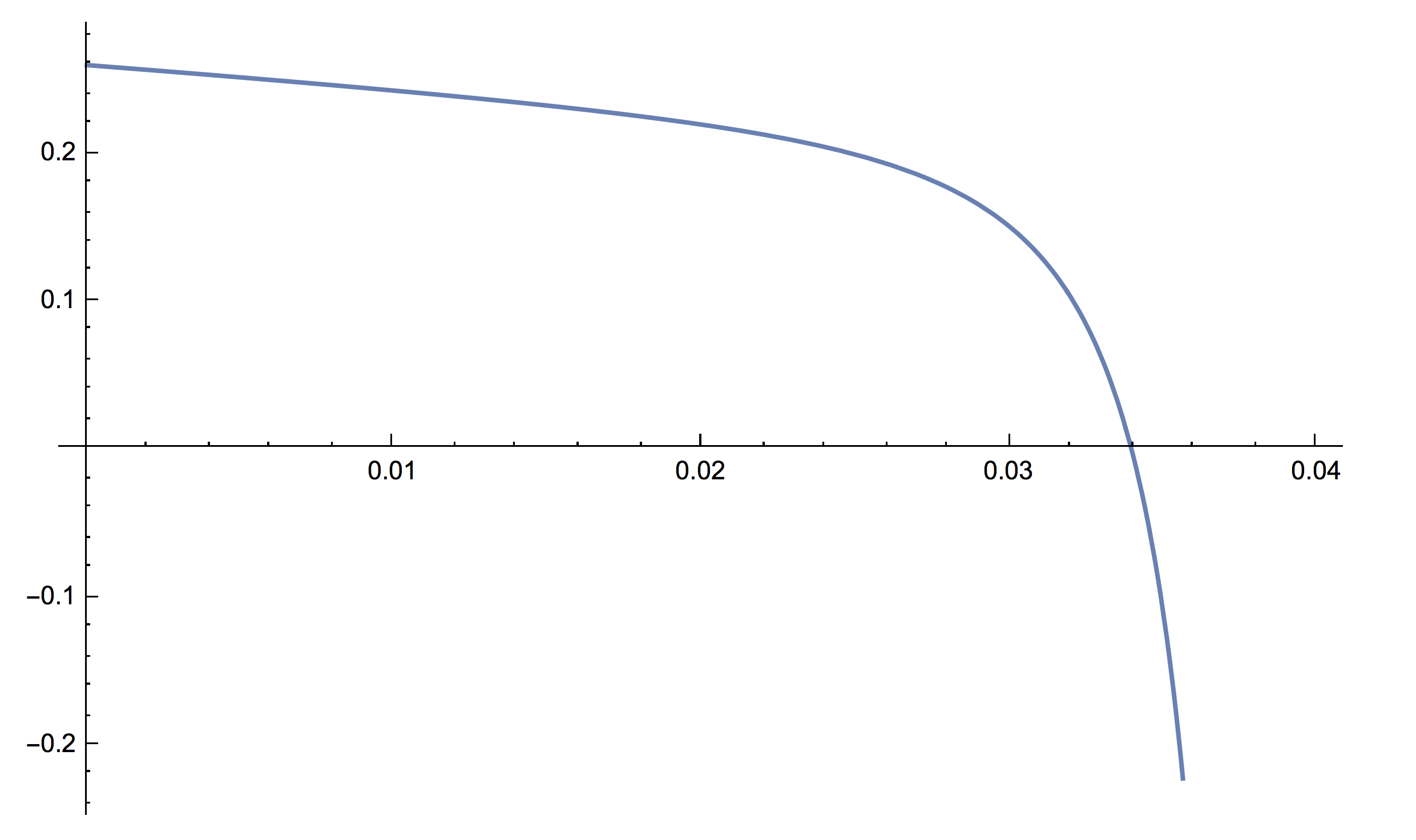
Q⁡(δ)=1.62π2​∫01.6cos2⁡(π1.6​s)​(δ+δ22​k​(s))​𝑑s∫01.6sin2⁡(π1.6​s)​log⁡(1+δ​k​(s))k⁡(s)​𝑑s−4​δ2(1−25​δ)2>0.Q(\delta)=\frac{1.6^{2}}{\pi^{2}}\frac{\displaystyle\int_{0}^{1.6}\cos^{2}\left(\frac{\pi}{1.6}s\right)\left(\delta+\frac{\delta^{2}}{2}k(s)\right)ds}{\displaystyle\int_{0}^{1.6}\sin^{2}\left(\frac{\pi}{1.6}s\right)\frac{\log(1+\delta k(s))}{k(s)}ds}-\frac{4\delta^{2}}{(1-25\delta)^{2}}>0.

We graph Q⁡(δ)Q(\delta) in Figure 33 below

Refer to caption
Figure 3. A graph of Q⁡(δ)Q(\delta) from Example 3.

and find using Mathematica that Q⁡(δ)>0Q(\delta)>0 provided δ<.03393\delta<.03393. We therefore have

μ1​(D)=μ1o​d​d​(D)≥π22.56​(1+5​δ)2\mu_{1}(D)=\mu_{1}^{odd}(D)\geq\frac{\pi^{2}}{2.56(1+5\delta)^{2}}

for such values of δ\delta.

4. Some considerations in the three-dimensional case

Let Ω\Omega be a bounded subset of ℝ2\mathbb{R}^{2} and let φ⁡(s,t)=(x⁡(s,t),y⁡(s,t),z⁡(s,t))\varphi(s,t)=\left(x(s,t),y(s,t),z(s,t)\right), (s,t)∈Ω(s,t)\in\Omega, be a smooth surface. Consider the three-dimensional domain DD consisting of the points on one side of φ\varphi, within a suitable distance δ\delta of φ\varphi. If we denote by ν=(νx,νy,νz)=φs×φt‖φs×φt‖\nu=(\nu_{x},\nu_{y},\nu_{z})=\dfrac{\varphi_{s}\times\varphi_{t}}{||\varphi_{s}\times\varphi_{t}||} a chosen unit normal vector to φ\varphi, DD can be described as follows:

(4.1) D={(x(s,t)+rνx(s,t),y(s,t)+rνy(s,t),z(s,t)+rνz(s,t)):(s,t)∈Ω,r∈(0,δ)}.D=\left\{\left(x(s,t)+r\nu_{x}(s,t),y(s,t)+r\nu_{y}(s,t),z(s,t)+r\nu_{z}(s,t)\right):\>(s,t)\in\Omega,\>r\in(0,\delta)\right\}.

In order to evaluate integrals over DD, we introduce a Fermi coordinate system using r=distφ(x,y,z)r=\mathop{\mathrm{dist}}\nolimits_{\varphi}(x,y,z) as one coordinate and s,ts,t, the coordinates in Ω\Omega of the point on φ\varphi nearest to (x,y,z)(x,y,z), as the other ones. The domains DD that we will consider arise from smooth surfaces φ\varphi that are generalized cylinders and surfaces of revolution.

4.1. Generalized cylinders

A generalized cylinder is a special case of a ruled surface, which is a surface that is a union of straight lines. We have a generalized cylinder when the straight lines, or rulings, are all parallel to each other. Given a set of parallel rulings, a parametrized curve α\alpha in ℝ3\mathbb{R}^{3} that meets each of these rulings, and a constant unit vector β\beta that is parallel to the rulings, the corresponding generalized cylinder may be described as

(4.2) φ⁡(s,t)=α⁡(s)+t​β,t∈ℝ.\varphi(s,t)=\alpha(s)+t\beta,\hskip 17.00024ptt\in\mathbb{R}.

It can be shown that we may always assume that α\alpha is parametrized with respect to arc length and contained in a plane that is perpendicular to β\beta. Without loss of generality, suppose that α⁡(s)=(x⁡(s),0,z⁡(s))\alpha(s)=(x(s),0,z(s)), s∈[0,L]s\in[0,L], is a smooth, non-closed, simple curve, parametrized with respect to its arc length, whose image is contained in the plane y=0y=0. Moreover, suppose α⁡(s)\alpha(s) is symmetric with respect to the zz-axis so that

x⁡(L−s)=−x⁡(s),z⁡(L−s)=z⁡(s),s∈[0,L2].x(L-s)=-x(s),\ \ z(L-s)=z(s),\hskip 8.50012pts\in\left[0,\frac{L}{2}\right].

Take β=(0,−1,0)\beta=(0,-1,0) and consider the surface φ\varphi given by (4.2) with s∈(0,L)s\in(0,L) and t∈(0,T)t\in(0,T) for some T>0T>0. A typical domain DD constructed from a generalized cylinder as in (4.1) is shown in Figure 44.

Refer to caption
Figure 4. A typical domain DD constructed from a generalized cylinder.

We see that {φs,φt,ν}\{\varphi_{s},\varphi_{t},\nu\} forms an orthonormal basis for ℝ3\mathbb{R}^{3}. Recalling notation from the appendix, we compute

E=|φs|2=1,\displaystyle E=|\varphi_{s}|^{2}=1, F=φs⋅φt=0,G=|φt|2=1,\displaystyle F=\varphi_{s}\cdot\varphi_{t}=0,\hskip 8.50012pt\hskip 8.50012ptG=|\varphi_{t}|^{2}=1,
a=F​M−L​GE​G−F2=−L=−φs​s⋅ν=k(s),\displaystyle a=\frac{FM-LG}{EG-F^{2}}=-L=-\varphi_{ss}\cdot\nu=k(s), b=L​F−E​ME​G−F2=−M=−φs​t⋅ν=0,\displaystyle b=\frac{LF-EM}{EG-F^{2}}=-M=-\varphi_{st}\cdot\nu=0,
c=F​N−M​GE​G−F2=0,\displaystyle c=\frac{FN-MG}{EG-F^{2}}=0, d=M​F−N​EE​G−F2=−N=−φt​t⋅ν=0,\displaystyle d=\frac{MF-NE}{EG-F^{2}}=-N=-\varphi_{tt}\cdot\nu=0,

where k⁡(s)k(s) is the curvature of α\alpha. Moreover, the Jacobian of the Fermi transformation is independent of tt:

det(J⁡(r,s,t))=det(J⁡(r,s))=1+a​r=1+r​k​(s).\det(J(r,s,t))=\det(J(r,s))=1+ar=1+rk(s).

With this setup, we can now give a lower bound on μ1o​d​d\mu_{1}^{odd} for generalized cylinders.

Theorem 4.1.

Suppose that the curvature k⁡(s)k(s) of α\alpha is concave in [0,L][0,L] and let δ>0\delta>0 be such that 1+δ​k​(s)>01+\delta k(s)>0 in [0,L][0,L]. If DD is simply connected and μ1o​d​d​(D)\mu_{1}^{odd}(D) is the smallest nontrivial Neumann eigenvalue having a corresponding eigenfunction that is odd with respect to the plane x=0x=0, we have

μ1o​d​d​(D)≥B​π2L2,\mu_{1}^{odd}(D)\geq B\frac{\pi^{2}}{L^{2}},

where B=min[0,δ]×[0,L]​1(1+r​k​(s))2B=\underset{[0,\delta]\times[0,L]}{\min}\frac{1}{(1+rk(s))^{2}}.

Proof.

We will argue as in the two-dimensional case. Fix n∈ℕn\in\mathbb{N}. For any i=0,…,n−1i=0,\dots,n-1, and any j=0,…,n−1j=0,\dots,n-1, let us denote by

Di​j={(x,y,z)∈D:i​δn<distφ(x,y,z)<(i+1)​δn,j​Tn<t<(j+1)​Tn}.D_{ij}=\left\{(x,y,z)\in D:\>\frac{i\delta}{n}<\mathop{\mathrm{dist}}\nolimits_{\varphi}(x,y,z)<\frac{(i+1)\delta}{n},\>\frac{jT}{n}<t<\frac{(j+1)T}{n}\right\}.

Let uu be an eigenfunction corresponding to μ1o​d​d​(D)\mu_{1}^{odd}(D) that is odd with respect to the plane x=0x=0. Using the definition of eigenfunction and a Green’s formula, we see that

μ1o​d​d​(D)=∫D|∇u|2​𝑑x​𝑑y​𝑑z∫Du2​𝑑x​𝑑y​𝑑z;\mu_{1}^{odd}(D)=\frac{\displaystyle\int_{D}|\nabla u|^{2}dxdydz}{\displaystyle\int_{D}u^{2}dxdydz};

moreover, the fact that uu is odd implies

∫Di​ju​𝑑x​𝑑y​𝑑z=0​for all ​i= 0,…,n−1​ and for all ​j=0,…,n−1.\int_{D_{ij}}u\,dxdydz=0\hskip 8.50012pt\text{for all }i=\ 0,\dots,n-1\text{ and for all }j=0,\dots,n-1.

We want to evaluate the energy of uu in any Di​jD_{ij}. Using the Fermi coordinate system and denoting 𝒥=|det(J)|\mathcal{J}=|\det(J)|, we have

∫Di​j|∇u|2​𝑑x​𝑑y​𝑑z\displaystyle\int_{D_{ij}}|\nabla u|^{2}dxdydz =\displaystyle= ∫0L(∫j​Tn(j+1)​Tn∫i​δn(i+1)​δn(ur2+us2​(1+d​r)2𝒥2+ut2​(1+a​r)2𝒥2)​𝒥​𝑑r​𝑑t)​𝑑s\displaystyle\int_{0}^{L}\left(\int_{\frac{jT}{n}}^{\frac{(j+1)T}{n}}\int_{\frac{i\delta}{n}}^{\frac{(i+1)\delta}{n}}\left(u_{r}^{2}+u_{s}^{2}\frac{(1+dr)^{2}}{\mathcal{J}^{2}}+u_{t}^{2}\frac{(1+ar)^{2}}{\mathcal{J}^{2}}\right)\,\mathcal{J}\,drdt\right)ds
≥\displaystyle\geq minDi​j⁡𝒥−2​∫0L(∫j​Tn(j+1)​Tn∫i​δn(i+1)​δnus2​𝒥​𝑑r​𝑑t)​𝑑s\displaystyle\min_{D_{ij}}\mathcal{J}^{-2}\int_{0}^{L}\left(\int_{\frac{jT}{n}}^{\frac{(j+1)T}{n}}\int_{\frac{i\delta}{n}}^{\frac{(i+1)\delta}{n}}u_{s}^{2}\,\mathcal{J}\,drdt\right)ds
≥\displaystyle\geq B​∫0L(∫j​Tn(j+1)​Tn∫i​δn(i+1)​δnus2​𝒥​𝑑r​𝑑t)​𝑑s.\displaystyle B\int_{0}^{L}\left(\int_{\frac{jT}{n}}^{\frac{(j+1)T}{n}}\int_{\frac{i\delta}{n}}^{\frac{(i+1)\delta}{n}}u_{s}^{2}\,\mathcal{J}\,drdt\right)ds.

Let us write

∫0L(∫j​Tn(j+1)​Tn∫i​δn(i+1)​δnus2​𝒥​𝑑r​𝑑t)​𝑑s=I1+I2,\int_{0}^{L}\left(\int_{\frac{jT}{n}}^{\frac{(j+1)T}{n}}\int_{\frac{i\delta}{n}}^{\frac{(i+1)\delta}{n}}u_{s}^{2}\,\mathcal{J}\,drdt\right)ds=I_{1}+I_{2},

where

I1\displaystyle I_{1} =\displaystyle= ∫0L(∫j​Tn(j+1)​Tn∫i​δn(i+1)​δn(us2​(r,s,t)−us2​(i​δn,s,j​Tn))​𝒥​(r,s,t)​𝑑r​𝑑t)​𝑑s,\displaystyle\int_{0}^{L}\left(\int_{\frac{jT}{n}}^{\frac{(j+1)T}{n}}\int_{\frac{i\delta}{n}}^{\frac{(i+1)\delta}{n}}\left(u_{s}^{2}(r,s,t)-u_{s}^{2}\left(\frac{i\delta}{n},s,\frac{jT}{n}\right)\right)\mathcal{J}(r,s,t)drdt\right)ds,
I2\displaystyle I_{2} =\displaystyle= ∫0L(∫j​Tn(j+1)​Tn∫i​δn(i+1)​δnus2​(i​δn,s,j​Tn)​𝒥​(r,s,t)​𝑑r​𝑑t)​𝑑s\displaystyle\int_{0}^{L}\left(\int_{\frac{jT}{n}}^{\frac{(j+1)T}{n}}\int_{\frac{i\delta}{n}}^{\frac{(i+1)\delta}{n}}u_{s}^{2}\left(\frac{i\delta}{n},s,\frac{jT}{n}\right)\mathcal{J}(r,s,t)drdt\right)ds
=\displaystyle= T​δn2​∫0Lus2​(i​δn,s,j​Tn)​(1+1+2​i2​δn​k​(s))​𝑑s.\displaystyle\frac{T\delta}{n^{2}}\int_{0}^{L}u_{s}^{2}\left(\frac{i\delta}{n},s,\frac{jT}{n}\right)\left(1+\frac{1+2i}{2}\frac{\delta}{n}k(s)\right)ds.

Analogously, it holds that

∫Di​ju2​𝑑x​𝑑y​𝑑z=∫0L(∫j​Tn(j+1)​Tn∫i​δn(i+1)​δnu2​𝒥​𝑑r​𝑑t)​𝑑s=H1+H2,\int_{D_{ij}}u^{2}dxdydz=\int_{0}^{L}\left(\int_{\frac{jT}{n}}^{\frac{(j+1)T}{n}}\int_{\frac{i\delta}{n}}^{\frac{(i+1)\delta}{n}}u^{2}\,\mathcal{J}drdt\right)ds=H_{1}+H_{2},

where

H1\displaystyle H_{1} =\displaystyle= ∫0L(∫j​Tn(j+1)​Tn∫i​δn(i+1)​δn(u2​(r,s,t)−u2​(i​δn,s,j​Tn))​𝒥​(r,s,t)​𝑑r​𝑑t)​𝑑s,\displaystyle\int_{0}^{L}\left(\int_{\frac{jT}{n}}^{\frac{(j+1)T}{n}}\int_{\frac{i\delta}{n}}^{\frac{(i+1)\delta}{n}}\left(u^{2}(r,s,t)-u^{2}\left(\frac{i\delta}{n},s,\frac{jT}{n}\right)\right)\mathcal{J}(r,s,t)drdt\right)ds,
H2\displaystyle H_{2} =\displaystyle= ∫0L(∫j​Tn(j+1)​Tn∫i​δn(i+1)​δnu2​(i​δn,s,j​Tn)​𝒥​(r,s,t)​𝑑r​𝑑t)​𝑑s\displaystyle\int_{0}^{L}\left(\int_{\frac{jT}{n}}^{\frac{(j+1)T}{n}}\int_{\frac{i\delta}{n}}^{\frac{(i+1)\delta}{n}}u^{2}\left(\frac{i\delta}{n},s,\frac{jT}{n}\right)\mathcal{J}(r,s,t)drdt\right)ds
=\displaystyle= T​δn2​∫0Lu2​(i​δn,s,j​Tn)​(1+1+2​i2​δn​k​(s))​𝑑s.\displaystyle\frac{T\delta}{n^{2}}\int_{0}^{L}u^{2}\left(\frac{i\delta}{n},s,\frac{jT}{n}\right)\left(1+\frac{1+2i}{2}\frac{\delta}{n}k(s)\right)ds.

Let AA be a common bound for the absolute value of each of uu and its first and second derivatives when expressed in Fermi coordinates. Applying the Mean Value Theorem, we deduce that

|I1|≤2​A2​(T+δ)n​|Di​j|,|H1|≤2​A2​(T+δ)n​|Di​j|.|I_{1}|\leq\frac{2A^{2}(T+\delta)}{n}|D_{ij}|,\hskip 8.50012pt|H_{1}|\leq\frac{2A^{2}(T+\delta)}{n}|D_{ij}|.

Using that k⁡(s)k(s) is even and uu is odd with respect to L2\frac{L}{2}, we see that

∫0Lu⁡(i​δn,s,j​Tn)​(1+1+2​i2​δn​k​(s))​𝑑s=0.\int_{0}^{L}u\left(\frac{i\,\delta}{n},s,\frac{jT}{n}\right)\left(1+\frac{1+2i}{2}\frac{\delta}{n}k(s)\right)ds=0.

Thus, arguing as in the two-dimensional case, we may apply Lemma 2.1 to conclude that I2≥π2L2​H2I_{2}\geq\dfrac{\pi^{2}}{L^{2}}H_{2}. We combine our estimates in a manner parallel to that of the two-dimensional case, summing over ii and jj; taking the limit as nn goes to +∞+\infty yields the result. ∎

Remark 4.1.

Let DD be constructed from a generalized cylinder as in Theorem 4.1. By separation of variables, the eigenvalues of DD take the form

μ⁡(D)=μm​(D~)+n2​π2T2,m,n≥0,\mu(D)=\mu_{m}(\widetilde{D})+\frac{n^{2}\pi^{2}}{T^{2}},\hskip 8.50012ptm,n\geq 0,

where D~\widetilde{D} is a two-dimensional domain in the x​zxz-plane as in (1.3). If TT is sufficiently large, then μ1​(D)=π2T2\mu_{1}(D)=\frac{\pi^{2}}{T^{2}} with corresponding eigenfunction u⁡(x,y,z)=cos⁡(π​yT)u(x,y,z)=\cos\left(\frac{\pi y}{T}\right). Observe that uu is odd with respect to the plane y=−T2y=-\frac{T}{2}. Thus as TT becomes large, we expect eigenfunctions for μ1​(D)\mu_{1}(D) to exhibit odd symmetry with respect to the plane y=−T2y=-\frac{T}{2} rather than the plane x=0x=0. On the other hand, if TT is sufficiently small, then μ1​(D)=μ1​(D~)\mu_{1}(D)=\mu_{1}(\widetilde{D}) and eigenfunctions for μ1​(D)\mu_{1}(D) take the form u⁡(x,y,z)=v⁡(x,z)u(x,y,z)=v(x,z), where vv is an eigenfunction for μ1​(D~)\mu_{1}(\widetilde{D}). Hence we may apply Proposition 3.2 to give conditions on δ\delta that guarantee μ1​(D~)=μ1o​d​d​(D~)\mu_{1}(\widetilde{D})=\mu_{1}^{odd}(\widetilde{D}) and therefore μ1​(D)=μ1o​d​d​(D)\mu_{1}(D)=\mu_{1}^{odd}(D).

4.2. Surfaces of revolution

Let α⁡(s)=(x⁡(s),0,z⁡(s)),s∈[0,L]\alpha(s)=(x(s),0,z(s)),s\in[0,L], be the curve considered in §4.1. We assume, without loss of generality, that x⁡(s)≥0x(s)\geq 0 for s∈[0,L2]s\in\left[0,\frac{L}{2}\right]. Our aim is to construct a three-dimensional domain DD consisting of certain points on one side of the surface of revolution obtained by a π\pi rotation of α\alpha around the zz-axis. We consider the surface

(4.3) φ⁡(s,θ)=(x⁡(s,θ),y⁡(s,θ),z⁡(s,θ))=(x⁡(s)​sin⁡θ,x⁡(s)​cos⁡θ,z⁡(s)),s∈(0,L2),θ∈(0,π),\varphi(s,\theta)=\left(x(s,\theta),y(s,\theta),z(s,\theta)\right)=\left(x(s)\sin\theta,x(s)\cos\theta,z(s)\right),\hskip 17.00024pts\in{\left(0,\frac{L}{2}\right),\>\theta\in(0,\pi)},

and the domain

D+={(x(s,θ)+rνx(s,θ),y(s,θ)+rνy(s,θ),z(s,θ)+rνz(s,θ)):(s,θ)∈(0,L2)×(0,π),r∈(0,δ)}.D_{+}=\left\{\left(x(s,\theta)+r\nu_{x}(s,\theta),y(s,\theta)+r\nu_{y}(s,\theta),z(s,\theta)+r\nu_{z}(s,\theta)\right):\>(s,\theta)\in\left(0,\frac{L}{2}\right)\times(0,\pi),\>r\in(0,\delta)\right\}.

Then, D=D+∪D−∪(int(∂D+∩{x=0}))D=D_{+}\cup D_{-}\cup(\textup{int}(\partial D_{+}\cap\{x=0\})), where D−D_{-} is the domain symmetric to D+D_{+} with respect to the y​zyz-plane, and int denotes the two-dimensional interior taken in the plane {x=0}\{x=0\}. Note that the parametrization of φ\varphi is not regular at s=L2s=\frac{L}{2} or at s=0s=0; we identify all points corresponding to each such ss-value and define ν\nu at those points by continuous extension. Had we done a rotation through π\pi of the whole curve α\alpha, we would have more serious issues with regularity. A typical domain DD constructed from a surface of revolution is shown in Figure 55.

Refer to caption
Figure 5. A typical domain DD constructed from a surface of revolution.

We see that {φs,φθ,ν}\{\varphi_{s},\varphi_{\theta},\nu\} forms an orthonormal basis for ℝ3\mathbb{R}^{3}. Recalling notation from the appendix, we compute

E=|φs|2=1,F\displaystyle E=|\varphi_{s}|^{2}=1,\hskip 8.50012ptF =\displaystyle= φs⋅φθ=0,G=|φθ|2=x​(s)2,\displaystyle\varphi_{s}\cdot\varphi_{\theta}=0,\hskip 8.50012ptG=|\varphi_{\theta}|^{2}=x(s)^{2},
a=F​M−L​GE​G−F2=−L=−φs​s⋅ν=k(s),\displaystyle a=\frac{FM-LG}{EG-F^{2}}=-L=-\varphi_{ss}\cdot\nu=k(s), b=L​F−E​ME​G−F2=−MG=−φs​θ⋅νG=0,\displaystyle b=\frac{LF-EM}{EG-F^{2}}=-\dfrac{M}{G}=-\dfrac{\varphi_{s\theta}\cdot\nu}{G}=0,
c=F​N−M​GE​G−F2=−M=−φs​θ⋅ν=0,\displaystyle c=\frac{FN-MG}{EG-F^{2}}=-M=-\varphi_{s\theta}\cdot\nu=0, d=M​F−N​EE​G−F2=−NG=−φθ​θ⋅νG=z′​(s)x⁡(s),\displaystyle d=\frac{MF-NE}{EG-F^{2}}=-\dfrac{N}{G}=-\dfrac{\varphi_{\theta\theta}\cdot\nu}{G}=\dfrac{z^{\prime}(s)}{x(s)},

where k⁡(s)k(s) is the curvature of α\alpha. Moreover, the Jacobian of the Fermi transformation is independent of θ\theta:

det(J⁡(r,s,θ))=det(J⁡(r,s))=(x⁡(s)+r​z′​(s))​(1+r​k​(s)).\det(J(r,s,\theta))=\det(J(r,s))=(x(s)+rz^{\prime}(s))(1+rk(s)).

With this setup, we may now give a lower bound on μ1o​d​d\mu_{1}^{odd} for surfaces of revolution.

Theorem 4.2.

Let δ>0\delta>0 be such that det(J⁡(r,s))>0\det(J(r,s))>0 on [0,δ]×(0,L2)[0,\delta]\times\left(0,\dfrac{L}{2}\right) and 1+δ​k​(s)>01+\delta k(s)>0 for s∈[0,L]s\in\left[0,L\right]. Suppose that for each r∈[0,δ]r\in[0,\delta], the function 𝒥⁡(r,s)=|det(J⁡(r,s))|\mathcal{J}(r,s)=|\det(J(r,s))| is concave in s∈[0,L2]s\in\left[0,\dfrac{L}{2}\right]. Assume DD is simply connected and denote by μ1o​d​d​(D)\mu_{1}^{odd}(D) the smallest nontrivial Neumann eigenvalue with a corresponding eigenfunction that is odd with respect to the plane x=0x=0. Then

(4.4) μ1o​d​d​(D)≥B​π2L2,\mu_{1}^{odd}(D)\geq B\frac{\pi^{2}}{L^{2}},

with B=min[0,δ]×[0,L]⁡1(1+r​k​(s))2.B=\displaystyle\min_{[0,\delta]\times[0,L]}\dfrac{1}{(1+rk(s))^{2}}.

In order to prove this theorem we need a variant of Lemma 2.1.

Lemma 4.1.

Let p⁡(s)p(s) be a concave, non-negative function on the interval [0,L2]\left[0,\frac{L}{2}\right] such that p⁡(L2)=0p\left(\dfrac{L}{2}\right)=0. Then for any piecewise twice differentiable function v⁡(s)v(s) that satisfies

v′​(0)=v⁡(L2)=0,v^{\prime}(0)=v\left(\dfrac{L}{2}\right)=0,

it follows that

∫0L2(v′​(s))2​p​(s)​𝑑s≥4​π2L2​∫0L2(v⁡(s))2​p​(s)​𝑑s.\int_{0}^{{\frac{L}{2}}}(v^{\prime}(s))^{2}p(s)ds\geq\frac{4\pi^{2}}{L^{2}}\int_{0}^{\frac{L}{2}}(v(s))^{2}p(s)ds.

The proof of Lemma 4.1 is similar to that of Lemma 2.1 (cf. [4], [19]). Note that v⁡(s)v(s) satisfies a singular Sturm-Liouville problem and that we may make a change of variables as in the original proof:

w=v′​p1/2.w=v^{\prime}p^{1/2}.

Since we are assuming that v′​(0)=v⁡(L2)=0v^{\prime}(0)=v\left(\dfrac{L}{2}\right)=0, we see that ww satisfies homogeneous Dirichlet boundary conditions and can thus serve as a test function in the Rayleigh quotient for a vibrating string of length L2\dfrac{L}{2} with fixed ends.

Proof of Theorem 4.2.

In addition to Lemma 4.1, we will use a slight modification of the arguments in the proof of Theorem 4.1. First, we observe that an eigenfunction uu corresponding to μ1o​d​d​(D)\mu_{1}^{odd}(D) is the first eigenfunction of the Laplace operator on D+D_{+} with mixed boundary conditions: Dirichlet on ∂D+∩{x=0}\partial D_{+}\cap\{x=0\} and Neumann on the remaining part of ∂D+\partial D_{+}. Fixing n∈ℕn\in\mathbb{N}, we partition D+D_{+} as

D+i​j={(x,y,z)∈D+:i​δn<distφ(x,y,z)<(i+1)​δn,j​πn<θ<(j+1)​πn},D_{+}^{ij}=\left\{(x,y,z)\in D_{+}:\>\frac{i\delta}{n}<\mathop{\mathrm{dist}}\nolimits_{\varphi}(x,y,z)<\frac{(i+1)\delta}{n},\>\frac{j\pi}{n}<\theta<\frac{(j+1)\pi}{n}\right\},\>

for i=0,…,n−1i=0,\dots,n-1 and j=0,…,n−1j=0,\dots,n-1. We observe that

(4.5) ∫Di​j+|∇u|2​𝑑x​𝑑y​𝑑z\displaystyle\int_{D_{ij}^{+}}|\nabla u|^{2}dxdydz =\displaystyle= ∫0L2(∫j​πn(j+1)​πn∫i​δn(i+1)​δn(ur2+us2​x2​(1+d​r)2𝒥2+uθ2​x2​(1+a​r)2𝒥2)​𝒥​𝑑r​𝑑θ)​𝑑s\displaystyle\int_{0}^{\frac{L}{2}}\left(\int_{\frac{j\pi}{n}}^{\frac{(j+1)\pi}{n}}\int_{\frac{i\delta}{n}}^{\frac{(i+1)\delta}{n}}\left(u_{r}^{2}+u_{s}^{2}\frac{x^{2}(1+dr)^{2}}{\mathcal{J}^{2}}+u_{\theta}^{2}\frac{x^{2}(1+ar)^{2}}{\mathcal{J}^{2}}\right)\mathcal{J}drd\theta\right)ds
≥\displaystyle\geq minDi​j+⁡x2​(1+d​r)2𝒥2​∫0L2(∫j​πn(j+1)​πn∫i​δn(i+1)​δnus2​𝒥​𝑑r​𝑑θ)​𝑑s\displaystyle\min_{D_{ij}^{+}}\frac{x^{2}(1+dr)^{2}}{\mathcal{J}^{2}}\int_{0}^{\frac{L}{2}}\left(\int_{\frac{j\pi}{n}}^{\frac{(j+1)\pi}{n}}\int_{\frac{i\delta}{n}}^{\frac{(i+1)\delta}{n}}u_{s}^{2}\mathcal{J}\,drd\theta\right)ds
≥\displaystyle\geq B​∫0L2(∫j​πn(j+1)​πn∫i​δn(i+1)​δnus2​𝒥​𝑑r​𝑑θ)​𝑑s,\displaystyle B\int_{0}^{\frac{L}{2}}\left(\int_{\frac{j\pi}{n}}^{\frac{(j+1)\pi}{n}}\int_{\frac{i\delta}{n}}^{\frac{(i+1)\delta}{n}}u_{s}^{2}\mathcal{J}\,drd\theta\right)ds,

where in the last line, we have used that x2​(1+d​r)2𝒥2=1(1+r​k​(s))2\frac{x^{2}(1+dr)^{2}}{\mathcal{J}^{2}}=\frac{1}{(1+rk(s))^{2}}. Let us write

∫0L2(∫j​πn(j+1)​πn∫i​δn(i+1)​δnus2​𝒥​𝑑r​𝑑θ)​𝑑s=I1+I2,\int_{0}^{\frac{L}{2}}\left(\int_{\frac{j\pi}{n}}^{\frac{(j+1)\pi}{n}}\int_{\frac{i\delta}{n}}^{\frac{(i+1)\delta}{n}}u_{s}^{2}\mathcal{J}\,drd\theta\right)ds=I_{1}+I_{2},

where

I1\displaystyle I_{1} =\displaystyle= ∫0L2(∫j​πn(j+1)​πn∫i​δn(i+1)​δn(us2​(r,s,θ)−us2​(i​δn,s,j​πn))​𝒥​𝑑r​𝑑θ)​𝑑s,\displaystyle\int_{0}^{\frac{L}{2}}\left(\int_{\frac{j\pi}{n}}^{\frac{(j+1)\pi}{n}}\int_{\frac{i\delta}{n}}^{\frac{(i+1)\delta}{n}}\left(u_{s}^{2}(r,s,\theta)-u_{s}^{2}\left(\frac{i\delta}{n},s,\frac{j\pi}{n}\right)\right)\mathcal{J}drd\theta\right)ds,
I2\displaystyle I_{2} =\displaystyle= ∫0L2(∫j​πn(j+1)​πn∫i​δn(i+1)​δnus2​(i​δn,s,j​πn)​𝒥​𝑑r​𝑑θ)​𝑑s\displaystyle\int_{0}^{\frac{L}{2}}\left(\int_{\frac{j\pi}{n}}^{\frac{(j+1)\pi}{n}}\int_{\frac{i\delta}{n}}^{\frac{(i+1)\delta}{n}}u_{s}^{2}\left(\frac{i\delta}{n},s,\frac{j\pi}{n}\right)\mathcal{J}drd\theta\right)ds
=\displaystyle= ∫0L2us2​(i​δn,s,j​πn)​p​(s)​𝑑s,\displaystyle\int_{0}^{\frac{L}{2}}u_{s}^{2}\left(\frac{i\delta}{n},s,\frac{j\pi}{n}\right)p(s)ds,

with

(4.6) p⁡(s)=∫j​πn(j+1)​πn∫i​δn(i+1)​δn𝒥⁡(r,s)​𝑑r​𝑑θ.p(s)=\int_{\frac{j\pi}{n}}^{\frac{(j+1)\pi}{n}}\int_{\frac{i\delta}{n}}^{\frac{(i+1)\delta}{n}}\mathcal{J}(r,s)\,drd\theta.

Analogously, it holds that

∫Di​j+u2​𝑑x​𝑑y​𝑑z=∫0L2(∫j​πn(j+1)​πn∫i​δn(i+1)​δnu2​(r,s,θ)​𝒥​𝑑r​𝑑θ)​𝑑s=H1+H2,\int_{D_{ij}^{+}}u^{2}dxdydz=\int_{0}^{\frac{L}{2}}\left(\int_{\frac{j\pi}{n}}^{\frac{(j+1)\pi}{n}}\int_{\frac{i\delta}{n}}^{\frac{(i+1)\delta}{n}}u^{2}(r,s,\theta)\mathcal{J}\,drd\theta\right)ds=H_{1}+H_{2},

where

H1\displaystyle H_{1} =\displaystyle= ∫0L2(∫j​πn(j+1)​πn∫i​δn(i+1)​δn(u2​(r,s,θ)−u2​(i​δn,s,j​πn))​𝒥​𝑑r​𝑑θ)​𝑑s,\displaystyle\int_{0}^{\frac{L}{2}}\left(\int_{\frac{j\pi}{n}}^{\frac{(j+1)\pi}{n}}\int_{\frac{i\delta}{n}}^{\frac{(i+1)\delta}{n}}\left(u^{2}(r,s,\theta)-u^{2}\left(\frac{i\delta}{n},s,\frac{j\pi}{n}\right)\right)\mathcal{J}drd\theta\right)ds,
H2\displaystyle H_{2} =\displaystyle= ∫0L2(∫j​πn(j+1)​πn∫i​δn(i+1)​δnu2​(i​δn,s,j​πn)​𝒥​𝑑r​𝑑θ)​𝑑s\displaystyle\int_{0}^{\frac{L}{2}}\left(\int_{\frac{j\pi}{n}}^{\frac{(j+1)\pi}{n}}\int_{\frac{i\delta}{n}}^{\frac{(i+1)\delta}{n}}u^{2}\left(\frac{i\delta}{n},s,\frac{j\pi}{n}\right)\mathcal{J}drd\theta\right)ds
=\displaystyle= ∫0L2u2​(i​δn,s,j​πn)​p​(s)​𝑑s.\displaystyle\int_{0}^{\frac{L}{2}}u^{2}\left(\frac{i\delta}{n},s,\frac{j\pi}{n}\right)p(s)ds.

Since 𝒥⁡(r,s)\mathcal{J}(r,s) is concave in s∈[0,L2]s\in\left[0,\dfrac{L}{2}\right] and 𝒥⁡(r,L2)=0\mathcal{J}\left(r,\dfrac{L}{2}\right)=0 for each rr, we see that p⁡(s)p(s) as defined in (4.6) satisfies the hypotheses of Lemma 4.1. The lemma gives a relationship between I2I_{2} and H2H_{2}, and the remainder of the proof follows that of Theorem 4.1. ∎

Example 4 (Half-spherical shell).

If α⁡(s)=(R​sin⁡(sR),0,−R​cos⁡(sR))\alpha(s)=\left(R\sin\left(\dfrac{s}{R}\right),0,-R\cos\left(\dfrac{s}{R}\right)\right), s∈[0,2​π​R]s\in[0,2\pi R], then for any δ>0\delta>0 we get the half spherical shell

D+={((r+R)sin(sR)sinθ,(r+R)sin(sR)cosθ,−(r+R)cos(sR)):r∈(0,δ),s∈[0,πR],θ∈(0,π)}.D_{+}=\left\{\left((r+R)\sin\left(\dfrac{s}{R}\right)\sin\theta,\>(r+R)\sin\left(\dfrac{s}{R}\right)\cos\theta,\>-(r+R)\cos\left(\dfrac{s}{R}\right)\right):\>r\in(0,\delta),s\in[0,\pi R],\theta\in(0,\pi)\right\}.

In this case, we have

1(1+r​k​(s))2=R2(r+R)2.\frac{1}{(1+rk(s))^{2}}=\frac{R^{2}}{(r+R)^{2}}.

In [16], Li proves that μ1​(D)\mu_{1}(D) has multiplicity 3. Thus μ1​(D)\mu_{1}(D) must correspond to the angular eigenfunctions in the usual separation of variables, and hence there is an odd eigenfunction associated to μ1​(D)\mu_{1}(D). Theorem 4.2 gives

μ1​(D)=μ1o​d​d​(D)≥14​(δ+R)2.\mu_{1}(D)=\mu_{1}^{odd}(D)\geq\frac{1}{4(\delta+R)^{2}}.

5. Appendix

Here we provide some details about the Fermi coordinate systems in two and three dimensions. For the two-dimensional computations, let γ⁡(s)=(x⁡(s),y⁡(s)),s∈[0,L],\gamma(s)=(x(s),y(s)),\>s\in[0,L], be a smooth, non-closed, simple curve, parametrized with respect to arc length. Let DD be a simply connected domain described with coordinates (r,s)(r,s) as in (1.3). Consider the coordinates X=X⁡(r,s)X=X(r,s) and Y=Y⁡(r,s),Y=Y(r,s), where

X\displaystyle X =x⁡(s)+r​y′​(s),\displaystyle=x(s)+ry^{\prime}(s),
Y\displaystyle Y =y⁡(s)−r​x′​(s).\displaystyle=y(s)-rx^{\prime}(s).

Recall that the signed curvature k⁡(s)k(s) is defined by

k⁡(s)=x′​(s)​y′′​(s)−y′​(s)​x′′​(s).k(s)=x^{\prime}(s)y^{\prime\prime}(s)-y^{\prime}(s)x^{\prime\prime}(s).

It is straightforward to verify that the Jacobian matrix is

J=∂(X,Y)∂(r,s)=(y′x′+r​y′′−x′y′−r​x′′).J=\frac{\partial(X,Y)}{\partial(r,s)}=\left(\begin{matrix}y^{\prime}&x^{\prime}+ry^{\prime\prime}\\ -x^{\prime}&y^{\prime}-rx^{\prime\prime}\end{matrix}\right).

Assuming that 1+δ​k​(s)>01+\delta k(s)>0 for s∈[0,L]s\in[0,L], we see that the absolute value may be dropped:

(5.1) 𝒥=|det(J)|=1+r​k​(s)>0​for every​s∈[0,L],r∈[0,δ].\mathcal{J}=|\det(J)|=1+rk(s)>0\hskip 8.50012pt\mbox{for every}\>s\in[0,L],\,r\in[0,\delta].

We explicitly observe that (5.1) and the Inverse Function Theorem imply that the Fermi coordinates from [0,δ]×[0,L][0,\delta]\times[0,L] to D¯\overline{D} are locally one-to-one. Moreover, since DD is simply connected, the Global Invertibility Theorem ensures that the Fermi coordinates are globally one-to-one. For smooth functions uu, we have

(5.2) ∫Du⁡(X,Y)​𝑑X​𝑑Y=∫0L∫0δu⁡(r,s)​(1+r​k​(s))​𝑑r​𝑑s.\int_{D}u(X,Y)dXdY=\int_{0}^{L}\int_{0}^{\delta}u(r,s)(1+rk(s))drds.

Similarly, one calculates

uX\displaystyle u_{X} =−11+r​k​(s)​(−x′​us+(r​x′′−y′)​ur),\displaystyle=-\frac{1}{1+rk(s)}\left(-x^{\prime}u_{s}+(rx^{\prime\prime}-y^{\prime})u_{r}\right),
uY\displaystyle u_{Y} =−11+r​k​(s)​(−y′​us+(x′+r​y′′)​ur),\displaystyle=-\frac{1}{1+rk(s)}\left(-y^{\prime}u_{s}+(x^{\prime}+ry^{\prime\prime})u_{r}\right),

from which one deduces

|∇u​(X,Y)|2=1(1+r​k​(s))2​us2+ur2.|\nabla u(X,Y)|^{2}=\frac{1}{(1+rk(s))^{2}}u_{s}^{2}+u_{r}^{2}.

In the three-dimensional case, let φ\varphi be a surface described as φ⁡(s,t)=(x⁡(s,t),y⁡(s,t),z⁡(s,t)),(s,t)∈Ω\varphi(s,t)=(x(s,t),y(s,t),z(s,t)),(s,t)\in\Omega with Ω\Omega a bounded domain in ℝ2\mathbb{R}^{2}. Let DD be a simply connected three-dimensional domain described with coordinates (r,s,t)(r,s,t) as in (4.1), and suppose that {φs,φt,ν}\{\varphi_{s},\varphi_{t},\nu\} forms an orthonormal basis for ℝ3\mathbb{R}^{3}. Consider the coordinates X=X⁡(r,s,t)X=X(r,s,t), Y=Y⁡(r,s,t)Y=Y(r,s,t) and Z=Z⁡(r,s,t)Z=Z(r,s,t), where

X\displaystyle X =x⁡(s,t)+r​νx​(s,t),\displaystyle=x(s,t)+r\nu_{x}(s,t),
Y\displaystyle Y =y⁡(s,t)+r​νy​(s,t),\displaystyle=y(s,t)+r\nu_{y}(s,t),
Z\displaystyle Z =z⁡(s,t)+r​νz​(s,t).\displaystyle=z(s,t)+r\nu_{z}(s,t).

The Jacobian matrix of this transformation is

J=∂(X,Y,Z)∂(r,s,t)=(νxxs+r​νx,sxt+r​νx,tνyys+r​νy,syt+r​νy,tνzzs+r​νz,szt+r​νz,t).J=\frac{\partial(X,Y,Z)}{\partial(r,s,t)}=\left(\begin{matrix}\nu_{x}&x_{s}+r\nu_{x,s}&x_{t}+r\nu_{x,t}\\ \nu_{y}&y_{s}+r\nu_{y,s}&y_{t}+r\nu_{y,t}\\ \nu_{z}&z_{s}+r\nu_{z,s}&z_{t}+r\nu_{z,t}\end{matrix}\right).

To simplify the computation of the determinant of this Jacobian, we recall some notation. Let

E=|φs|2,F\displaystyle E=|\varphi_{s}|^{2},\hskip 8.50012ptF =φs⋅φt,G\displaystyle=\varphi_{s}\cdot\varphi_{t},\hskip 8.50012ptG =|φt|2,\displaystyle=|\varphi_{t}|^{2},
L=φs​s⋅ν,M\displaystyle L=\varphi_{ss}\cdot\nu,\hskip 8.50012ptM =φs​t⋅ν,N\displaystyle=\varphi_{st}\cdot\nu,\hskip 8.50012ptN =φt​t⋅ν,\displaystyle=\varphi_{tt}\cdot\nu,
a=F​M−L​GE​G−F2,\displaystyle a=\frac{FM-LG}{EG-F^{2}}, b=L​F−E​ME​G−F2,\displaystyle b=\dfrac{LF-EM}{EG-F^{2}},
c=F​N−M​GE​G−F2,\displaystyle c=\frac{FN-MG}{EG-F^{2}}, d=M​F−N​EE​G−F2,\displaystyle d=\dfrac{MF-NE}{EG-F^{2}},
H\displaystyle H =−a+d2=L​G+N​E−2​M​F2​(E​G−F2)mean curvature,\displaystyle=-\dfrac{a+d}{2}=\dfrac{LG+NE-2MF}{2(EG-F^{2})}\hskip 17.00024pt\mbox{mean curvature,}
K\displaystyle K =ad−bc=L​N−M2E​G−F2Gauss curvature.\displaystyle=ad-bc=\dfrac{LN-M^{2}}{EG-F^{2}}\hskip 17.00024pt\mbox{Gauss curvature}.

We can simplify

det(J)\displaystyle\det(J) =\displaystyle= ν⋅[(φs+r​νs)×(φt+r​νt)]\displaystyle\nu\cdot\left[\left(\varphi_{s}+r\nu_{s}\right)\times\left(\varphi_{t}+r\nu_{t}\right)\right]
=\displaystyle= φs×φt‖φs×φt‖⋅[(φs+r​νs)×(φt+r​νt)]\displaystyle\frac{\varphi_{s}\times\varphi_{t}}{||\varphi_{s}\times\varphi_{t}||}\cdot\left[\left(\varphi_{s}+r\nu_{s}\right)\times\left(\varphi_{t}+r\nu_{t}\right)\right]

using properties of the dot and cross products. In addition to well-known properties, we use Lagrange’s identity, which states that (𝐚×𝐛)⋅(𝐜×𝐝)=(𝐚⋅𝐜)​(𝐛⋅𝐝)−(𝐚⋅𝐝)​(𝐛⋅𝐜)(\mathbf{a}\times\mathbf{b})\cdot(\mathbf{c}\times\mathbf{d})=(\mathbf{a}\cdot\mathbf{c})(\mathbf{b}\cdot\mathbf{d})-(\mathbf{a}\cdot\mathbf{d})(\mathbf{b}\cdot\mathbf{c}) for vectors 𝐚,𝐛,𝐜,𝐝\mathbf{a},\mathbf{b},\mathbf{c},\mathbf{d}. We obtain

𝒥=|det(J)|=(1−2​r​H+r2​K)​(E​G−F2)1/2;\mathcal{J}=|\det(J)|=\left(1-2rH+r^{2}K\right)\left(EG-F^{2}\right)^{1/2};

here we have assumed 1−2​r​H+r2​K>01-2rH+r^{2}K>0 in order to drop the absolute values. Thus for a smooth function uu, we have

(5.4) ∫Du⁡(X,Y,Z)​𝑑X​𝑑Y​𝑑Z=∫0L∫0T∫0δu⁡(r,s,t)​(1−2​r​H+r2​K)​(E​G−F2)1/2​𝑑r​𝑑t​𝑑s.\int_{D}u(X,Y,Z)dXdYdZ=\int_{0}^{L}\int_{0}^{T}\int_{0}^{\delta}u(r,s,t)\left(1-2rH+r^{2}K\right)\left(EG-F^{2}\right)^{1/2}drdtds.

Finally, we need to express |∇u​(X,Y,Z)|2|\nabla u(X,Y,Z)|^{2} with respect to Fermi coordinates. We first compute

ur\displaystyle u_{r} =\displaystyle= ∇u⋅ν,\displaystyle\nabla u\cdot\nu,
us\displaystyle u_{s} =\displaystyle= ∇u⋅φs+r(∇u⋅νs),\displaystyle\nabla u\cdot\varphi_{s}+r(\nabla u\cdot\nu_{s}),
ut\displaystyle u_{t} =\displaystyle= ∇u⋅φt+r(∇u⋅νt).\displaystyle\nabla u\cdot\varphi_{t}+r(\nabla u\cdot\nu_{t}).

Then the reader may verify that, using the notation given in (5),

νs=a​φs+b​φt\displaystyle\nu_{s}=a\varphi_{s}+b\varphi_{t}\hskip 8.50012pt\hskip 8.50012pt and νt=c​φs+d​φt,\displaystyle\hskip 8.50012pt\hskip 8.50012pt\nu_{t}=c\varphi_{s}+d\varphi_{t},
∇u⋅φs=(1+d​r)​us−b​r​ut1−2​r​H+r2​K\displaystyle\nabla u\cdot\varphi_{s}=\frac{(1+dr)u_{s}-bru_{t}}{1-2rH+r^{2}K}\hskip 8.50012pt and ∇u⋅φt=(1+a​r)​ut−c​r​us1−2​r​H+r2​K.\displaystyle\hskip 8.50012pt\nabla u\cdot\varphi_{t}=\frac{(1+ar)u_{t}-cru_{s}}{1-2rH+r^{2}K}.

Combining these expressions and making the additional assumption that b=c=0b=c=0, we obtain

|∇u|2=ur2+us2​(1+d​r)2(1−2​r​H+r2​K)2+ut2​(1+a​r)2(1−2​r​H+r2​K)2.|\nabla u|^{2}=u_{r}^{2}+u_{s}^{2}\frac{(1+dr)^{2}}{(1-2rH+r^{2}K)^{2}}+u_{t}^{2}\frac{(1+ar)^{2}}{(1-2rH+r^{2}K)^{2}}.

Acknowledgements. B.B. and F.C. would like to thank the Department of Mathematics at Bucknell University for warm hospitality and support. E.B.D. was partially supported by a grant from the Simons Foundation (210445). J.J.L. appreciates the funding he received from Bucknell University’s International Research Travel Grants program. The authors would like to thank the anonymous referee for carefully reading the manuscript and for suggesting changes that strengthened the paper.

References

  • [1] M. S. Ashbaugh and F. Chiacchio, On low eigenvalues of the Laplacian with mixed boundary conditions, J. Differential Equations 250 (2011), 2544–2566.
  • [2] C. Bandle, Isoperimetric inequalities and applications. Monographs and Studies in Mathematics, 7. Pitman (Advanced Publishing Program), Boston, Mass.–London, 1980.
  • [3] R. Ban~\tilde{\rm n}uelos and K. Burdzy, On the “hot spots” conjecture of J. Rauch, J. Funct. Anal. 164 (1999), no. 1, 1–33.
  • [4] M. Bebendorf, A note on the Poincaré inequality for convex domains, Z. Anal. Anwendungen 22 (2003), no. 4, 751–756.
  • [5] B. Brandolini, F. Chiacchio and C. Trombetti, Sharp estimates for eigenfunctions of a Neumann problem, Comm. Partial Differential Equations 34 (2009), no. 10-12, 1317–1337.
  • [6] B. Brandolini, F. Chiacchio and C. Trombetti, A sharp lower bound for some Neumann eigenvalues of the Hermite operator, Differential Integral Equations 26 (2013), no. 5-6, 639–654.
  • [7] B. Brandolini, F. Chiacchio and C. Trombetti, Optimal lower bounds for eigenvalues of linear and nonlinear Neumann problems, Proc. Roy. Soc. Edinburgh Sect. A 145 (2015), no. 1, 31–45.
  • [8] A. Burchard and L. E. Thomas, On an isoperimetric inequality for a Schrödinger operator depending on the curvature of a loop, J. Geom. Anal. 15 (2005), no. 4, 543–563.
  • [9] L. A. Caffarelli and A. Friedman, Partial regularity of the zero-set of solutions of linear and superlinear elliptic equations, J. Differential Equations 60 (1985), no. 3, 420–433.
  • [10] P. Exner, P. Freitas and D. Krejčirík, A lower bound to the spectral threshold in curved tubes, Proc. R. Soc. Lond. Ser. A Math. Phys. Eng. Sci. 460 (2004), no. 2052, 3457–3467.
  • [11] P. Exner, E. M. Harrell and M. Loss, Optimal eigenvalues for some Laplacians and Schrödinger operators depending on curvature, Mathematical results in quantum mechanics (Prague, 1998), 47–58, Oper. Theory Adv. Appl., 108, Birkhäuser, Basel, 1999.
  • [12] V. Ferone, C. Nitsch and C. Trombetti, A remark on optimal weighted Poincaré inequalities for convex domains, Atti Accad. Naz. Lincei Rend. Lincei Mat. Appl. 23 (2012), no. 4, 467–475.
  • [13] V. Gol’dshtein and A. Ukhlov, On the first eigenvalues of free vibrating membranes in conformal regular domains, Arch. Rational Mech. Anal. (DOI) 10.1007/s00205-016-0988-9.
  • [14] A. Henrot, Extremum problems for eigenvalues of elliptic operators. Frontiers in Mathematics. Birkhäuser Verlag, Basel, 2006.
  • [15] D. Jerison, Locating the first nodal line in the Neumann problem, Trans. Amer. Math. Soc. 352 (2000), no. 5, 2301–2317.
  • [16] L. Li, On the second eigenvalue of the Laplacian in an annulus, Illinois J. Math. 51 (2007), no. 3, 913–925.
  • [17] V. G. Maz’ja, Sobolev spaces. Translated from the Russian by T. O. Shaposhnikova. Springer Series in Soviet Mathematics. Springer-Verlag, Berlin, 1985.
  • [18] P. L. Lions and F. Pacella, Isoperimetric inequalities for convex cones, Proc. Amer. Math. Soc. 109 (1990), (2) 477–485.
  • [19] L.E. Payne and H. F. Weinberger, An optimal Poincaré inequality for convex domains, Arch. Rational Mech. Anal., 5 (1960), 286–292.
  • [20] D. Valtorta, Sharp estimate on the first eigenvalue of the pp-Laplacian, Nonlin. Analysis 75 (2012), 4974–4994.