Fluctuations of the multiplicity of produced particles in onium-nucleus collisions
Abstract
We address the general features of event-by-event fluctuations of the multiplicity of gluons produced in the scattering of a dilute hadron off a large nucleus at high energy in the fragmentation region of the dilute hadron. We relate these fluctuations to the stochasticity of the number of quanta contained in the hadron at the time of the interaction. For simplicity, we address the ideal case in which the hadron is an onium, and investigate different kinematical regimes in rapidity and onium size. We show that at large rapidity, the multiplicity distribution exhibits an exponential tail in the large-multiplicity region, which is qualitatively consistent with the proton-nucleus data. But interestingly enough, the exponential shape is determined by confinement.
1 Introduction
The large amount of data collected at the RHIC and at the LHC has made accessible the
study of event-by-event fluctuations of a number of measurable quantities,
such as particle multiplicities in proton-nucleus and nucleus-nucleus
collisions.
The microscopic origin of the observed stochasticity is however not clear, and various
interpretations and phenomenological models have been proposed.
In the available models to date,
the stochasticity is often correlated to the
event-by-event fluctuations of the matter density in the nucleus.
(For a recent review on quantum fluctuations in
the initial state of heavy-ion collisions, see e.g. [1]).
A common assumption is that the nucleus is a set of nucleons
whose positions in the transverse plane relative to its center
are random, see for example the PHOBOS Glauber Monte Carlo model [2].
The flow of particles which go to the final state is then related
to the geometry of the initial nucleus.
Other recent models assume that the density of gluons significantly
fluctuates from nucleon to nucleon, and that these
fluctuations are encoded in the large-rapidity fluctuations of the saturation
scale [3]. However, such effects were shown,
theoretically [4] as well as phenomenologically [5],
to be small at realistic collider energies.
In this paper, we investigate the assumption that the fluctuations of the multiplicity of the produced particles
in the forward rapidity region of the proton in proton-nucleus collisions is entirely due to the event-by-event
fluctuations of the gluon content in the proton generated by the small- evolution, which
are known to be large (see e.g. the recent work of Ref. [6]).
The nucleus is instead a non-fluctuating object.
Indeed, we observe that generally speaking,
it is quite unnatural to have configurations
of nucleons inside the nucleus which are very different from uniformly distributed
since the wavefunction of a large nucleus is approximately the same as the
ground-state wavefunction of nuclear matter, for which it is known that density
fluctuations are very small [7].
Our paper is organized as follows. In the next section, we expose our picture of multiplicity fluctuations, relating them to the parton number fluctuations in the initial state of the dilute object. In Sec. 3, we provide the necessary background on small- evolution in the Balitsky-Fadin-Kuraev-Lipatov (BFKL) [8, 9, 10] regime, and in particular, we rederive the set of equations obeyed by the moments of the gluon number in the framework of the color dipole model [11]. In Sec. 4, we review the collinear, or double-logarithmic (DL) limit of these equations, relevant when the rapidity is large compared to the logarithm of the ratio of the relevant transverse scales, and solve them to obtain the multiplicity distribution. In Sec. 5, we release the DL approximation: The result of this plain BFKL calculation will prove unphysical, a problem that we shall address in the subsequent section 6. The concluding section contains some prospects, while two appendices discuss small- evolution in the diffusive approximation (Appendix A), and a numerical study of a dimensionally-reduced model which should share the main features of the full BFKL evolution (Appendix B).
2 Picture of the multiplicity fluctuations
As announced in the Introduction,
we shall concentrate on particle production in onium-nucleus collisions
in the fragmentation region of the onium. We will argue that
in this process, the shape of the multiplicity
distribution in a specific kinematical region that we
shall define properly below can be traced back to the fluctuations
of the number of quanta in the wavefunction of the onium
at the time of its interaction with the nucleus [12].
Our aim is not to build a realistic model for real hadron-nucleus
scattering, but rather to study in as many details as possible
onium (namely dipole)-nucleus scattering and derive, in this simple case, the
distribution of the number of particles (actually gluons) in the final state.
We expect that the main characteristics of the distribution we will find go
over unchanged to the experimentally measurable proton-nucleus
or deuterium-nucleus scattering processes.
This very kind of statistical fluctuations of the partonic content
of hadrons has been considered before: Their impact on the shape
and energy evolution of deep-inelastic scattering cross sections
was investigated in the deep saturation regime [13]
and at more moderate energies [14] (for
reviews, see [15, 16]).
Here, we consider the effect of these fluctuations on a final-state observable.
Throughout our work,
the nucleus will be characterized by one single momentum scale
, its
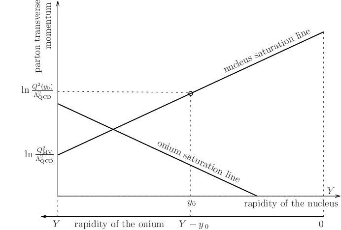
saturation scale, which depends on its rapidity
in the considered frame (see Fig. 1).
The latter scale just sets the upper
bound on the transverse momentum of the gluons
in the onium wavefunction that are freed and go to the final state.
Indeed, for an onium moving along the positive axis of a frame in which it has the lightcone momentum and in the corresponding gauge, particles are produced as follows:11 1 See e.g. Ref. [17] for a good review on high-energy scattering and on particle production Gluons in the wavefunction of the initial onium that have a transverse momentum smaller than the saturation momentum of the nucleus undergo multiple scatterings with the nucleus and are freed, while the nucleus will essentially be transparent to gluons with transverse momenta larger than the nuclear saturation scale. The mean multiplicity of the produced gluons per unit rapidity measured at central rapidity is related to the distribution of gluons in the onium of lightcone momentum integrated up to the transverse momentum scale as follows22 2 , where the last equality stems from the mass-shell condition . The first factor is then the exponential of the rapidity of the measured gluon relative to the rapidity of the nucleus, namely . An equivalent formula is , where is the mass of the onium. [18, 19]:
| (1) |
Formula (1) relates expectation values, namely mean quantities, where the averages are taken over events. In a given event, just before the collision occurs, the incoming onium is found in a particular Fock state (essentially made of gluons if its rapidity is large enough). The number of gluons and their momenta are random variables whose values fluctuate from event to event. We are going to assume that an equation similar to Eq. (1) holds as an identity between the random variables “number of produced particles per unit rapidity in the particular considered event” and “number of gluons in the corresponding realization of the quantum evolution of the onium”. Then the distribution of the multiplicity of particles produced is tantamount to the distribution of the gluon number in the particular realization of the partonic content of the onium at the time of its interaction with the nucleus.
We will choose the frame (namely the rapidity of the nucleus) in such a way that the onium (which has the rapidity ) appears as a dilute object whose state develops through a (linear) branching process, while the nucleus is characterized by a large saturation scale , see Fig. 1. In the next section, we shall review small- evolution in the linear regime.
3 Background on the small- evolution in the linear regime
Throughout, we will use the large number-of-color limit which will
enable us to always represent the partonic content
of the onium by a set of color dipoles [11].
We consider the set of
dipoles generated by small- evolution
starting with a dipole of size , which is our initial condition.
Our goal in this paper amounts to computing
the probability to observe a number of dipoles of size
larger than at some rapidity in one event, starting the evolution
from a single dipole.
At double logarithmic accuracy33 3 The most straightforward way to check Eq. (2) is to compare the explicit expressions its left and right-hand sides. In the double-log approximation, the gluon density reads , while the formula for is rederived below, see Eq. (24). , there is a simple relation between the ordinary (namely integrated) gluon density that appears in Eq. (1) and the first moment of :
| (2) |
where is the dipole number averaged over the events:
.
We shall assume that this relation would also hold as
an identity between the gluon density and the rate of evolution of
the dipole number with the rapidity in each realization of the quantum evolution.
We start by discussing the QCD evolution in the dipole model. Then, we establish the evolution equations for the dipole number.
3.1 QCD evolution and dipole branching
The QCD evolution results from the branching of the dipoles when the longitudinal phase space opens, namely when the rapidity grows. This branching is due to the emission of a gluon at position in the transverse plane from one of the endpoints of the dipoles, at respective positions and . The rate of emission, per unit rapidity and transverse surface , is given by the BFKL kernel
| (3) |
where is the size of the corresponding dipole. If one is not interested in the absolute position of the dipoles in the transverse plane but only in their sizes, then it is useful to express this rate as a rate of emission per unit size and rapidity:
| (4) |
This formula holds whenever the distances , and
may represent the length of the edges of a triangle, and if this
condition is not verified.
is interpreted as the probability
that a dipole of size split to two dipoles of sizes
and respectively (up to and resp.) when
the rapidity increases by .
Finally, it will prove convenient to introduce logarithmic dipole sizes . In this case, the splitting probability reads , where
| (5) |
Note that due to scale invariance, the kernel effectively depends on two independent real variables only.
3.2 Dipole number
Let us introduce the probability of having dipoles of size larger than after evolution over the rapidity , starting with a single dipole of size . It is easy to establish an equation for . To this aim, we assume that is known for all and all and we express , merely translating the branching process described in Sec. 3.1 into an equation:
| (6) |
Hence
| (7) |
This system of equations for the set of ’s may be represented by a single equation for the generating function of the factorial moments of the dipole number, which is defined as
| (8) |
Indeed, is easily seen to obey the Balitsky-Kovchegov (BK) equation44 4 Strictly speaking, the BK equation was established as an equation for the -matrix element for the forward elastic scattering of a dipole off a large nucleus. The evolution of the generating function we discuss here was first addressed in Ref. [11]. The two evolution equations can be written in the very same form. [20, 21]
| (9) |
Since the initial condition is a single dipole of size , then obviously
| (10) |
We also have
| (11) |
from the unitarity relation .
The factorial moments of the dipole numbers are obtained from by derivation with respect to the dummy variable :
| (12) |
Applying times the derivation operator to the BK equation (9), we see that the set of the factorial moments solves a hierarchy of integro-differential equations:
| (13) |
The equation for is the dipole version of the usual BFKL equation for the mean gluon number. Taking into account the initial condition (single dipole of size ), its solution reads55 5 Note that with our definition of , it only depends on the dipole size and not on its orientation nor on the position of its center in the transverse plane. The solution to the BFKL equation we give here is restricted to zero conformal spin.
| (14) |
where .
The higher moments obey an evolution equation which has the same kernel as the BFKL equation, but with a nontrivial source term represented by the inhomogeneous term in Eq. (13).
3.3 Integral expression for the higher moments
It is useful to introduce the number density of dipoles of transverse size present in the system after evolution of an initial dipole of size over units of rapidity. We define in such a way that
| (15) |
is the integrated number of dipoles. The mean dipole number density reads
| (16) |
We can readily express with the help of and . One easily checks66 6 Take for instance the derivative of Eq. (17) with respect to and identify its r.h.s. to the r.h.s. of the evolution equation for in Eq. (13) with . that the following formula holds true:
| (17) |
As for the higher moments of , similar equations may be written to express with the help of the ’s with The existence of such recursion relations is of course just related to the tree structure of the dipole evolution.
4 Collinear limit
Let us first study the collinear limit
in which is much smaller than the size
of the initial dipole.
The dominant contribution to the moments of the dipole number
is given by the configurations in which successive
dipole splittings are strongly ordered in size,
namely and
or and .
This translates into inequalities for the logarithmic dipole sizes
introduced above in Sec. 3.1, and
or and .
Technically, the BFKL kernel boils down to a uniform
distribution in the logarithm of the dipole sizes:
.
We write and use logarithmic variables as the argument of that represents the dipole sizes. The BK equation (9) simplifies to
| (18) |
The upper bound on the integration implements the fact that a dipole of a given size cannot split to larger dipoles in the collinear limit.
4.1 Moments of the dipole number
In the same manner as in Sec. 3, the equations for the factorial moments of the dipole number are easily obtained by taking derivatives of the BK equation in the collinear limit (18) with respect to , at :
| (19) |
namely
| (20) |
For the purpose of trying to understand the properties of the solutions to the hierarchy (19), it is convenient to start over with Eq. (18) and to rewrite it as a second-order partial differential equation
| (21) |
The left-hand side is a second derivative of the generating function of the factorial cumulants of the dipole multiplicity, connected to the factorial moments through the relations
| (22) |
Introducing further the variables and , the differential operator becomes . We then see that it is consistent to look for solutions which are independent of the variable : We will focus on such solutions in what follows. To obtain the differential equations in terms of the variable, it is convenient to start from Eq. (21) and take again derivatives with respect to
| (23) |
We note that the operator appearing in the homogeneous part of these equations is
the kernel of a Bessel equation.
The solution to the hierarchy cannot be expressed fully analytically,
however, the large- asymptotics are simple and
partially known.
Indeed, the same kind of equations appear in the context
of jet physics [22, 23].
Let us nevertheless discuss these asymptotics in some detail.
The solution of the equation for the first cumulant (or moment) with the initial condition is a modified Bessel function of the first kind:
| (24) |
The first moment is the mean dipole number. Another
notation for that we shall use in what follows
is .
The next equations in the hierarchy are seen to exhibit the same kernel as the equation for : Only the inhomogeneous term differs. As for , we find an exact expression which, once re-expressed in terms of moments through Eq. (22), reads
| (25) |
The above integrals do not have a simpler expression, however, we may obtain the large- expansion of from the expansion of the Bessel functions:
| (26) |
To first order in and switching back to the variables, we get
| (27) |
We may repeat this procedure for the higher moments. For example we find for :
| (28) |
The generic structure is
| (29) |
where the coefficients are constants.
The coefficients may be computed by inserting the Ansatz into the hierarchy (19), and by recalling that . The are then seen to obey the following recursion [22]:
| (30) |
For large , converges77 7 It is straightforward to check this asymptotic form for the solution by inserting it into Eq. (30). The value of the constant is obtained numerically. fastly to , where .
4.2 Multiplicity distribution
From the knowledge of the large- and large- asymptotics of the factorial moments (and hence of the ordinary moments, due to the exponential increase of at large ), one can infer the large- behavior of the distribution of the dipole multiplicity . Indeed,
| (31) |
where the second approximate equality holds for large , since the sum
over is dominated by large values of in that limit.
We continue analytically the moment index to complex values, and invert this equation as
| (32) |
which when we specialize to the collinear limit reads
| (33) |
A straightforward calculation leads to the final result
| (34) |
Note that the probability distribution
exhibits Koba-Nielsen-Olesen (KNO)
scaling [24], namely
is a function of
only.
One may think that the qualitative properties of this distribution would be kept when one gives up the strong ordering of the transverse momenta. This is actually not at all the case, as we will demonstrate in the next section.
5 Full BFKL evolution
When the ordering condition between and is released,
then the full BK equation has to be solved.
The difference between the full BK equation (9)
and its DL approximation (18) is that the former
allows splittings to larger dipoles, while the latter describes
only splittings to smaller dipoles.
We shall now review the asymptotics of the solution, which were first derived in Ref. [25], and interpret them. The most convenient is to analyze the equations for the moments. Let us start by discussing the second-order factorial moment .
5.1 Second-order moment
The second-order factorial moment is obtained by inserting the expressions of the first moments (14),(16) into Eq. (17). Using the logarithmic variables and , can be cast as
| (35) |
where
| (36) |
and
| (37) |
( and ).
We want to evaluate in the limit of large
and large .
We start by looking for a saddle point in the , and variables independently, and being fixed for the time being. We require that the partial derivative of with respect to these variables vanish, which leads to the unique solution
| (38) |
Performing this integral by the steepest-descent method, the pair multiplicity reads
| (39) |
where is the matrix of the second derivatives of
evaluated at the saddle point.
The saddle point depends on and on , over which we still need to integrate. We are going to search for a stationary point of in the two remaining integration variables and . The partial derivatives of with respect to and taken at the saddle point read
| (40a) | ||||
| (40b) | ||||
5.1.1 Global saddle point
For a global saddle point of the multiple integral to exist, the derivatives in Eq. (40) must vanish simultaneously, which requires
| (41) |
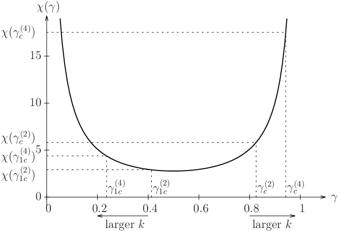
Eq. (41) can be solved numerically: . The solution is represented in Fig. 2. We note that and . Once the value of is fixed, Eq. (38) implies
| (42) |
We note that this solution requires to be negative. Conversely, if , then this saddle point solution exists provided , a condition that is satisfied whenever the external parameters obey the ordering relation
| (43) |
which follows from the first equation in (42), conveniently rewritten as
| (44) |
and from the negativity of the second term in the r.h.s.
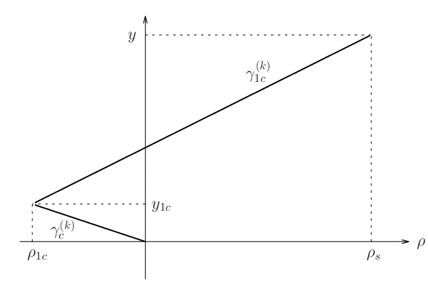
The physical picture of this solution is the following: Starting from the dipole of size , the first part of the evolution, which typically takes place over the first units of rapidity, produces a larger dipole (since is negative). The latter decays to two dipoles, which subsequently evolve independently over the rapidity range . The saddle-point solution is represented on the graph of the -function in Fig. 2, together with the evolution path in the plane.
5.1.2 Connection with the DL limit
If the global saddle-point solution does not exist, then
the values of
that contribute to the integration in Eq. (35)
are essentially positive.
In this case, the saddle point equations (38)
impose that both and be less than .
We can require again the stationarity of
with respect to the variations of ,
which, using (40a), leads to
the condition .
Hence , which
trivially implies .
Then, according to Eq. (40b)
the integral is strongly dominated by the region .
Indeed, an upper bound for the values of
which contribute significantly
to the integral is88
8
This bound may be derived
from the form of the -dependence of
(see Eq. (40b)) and
from the convexity properties
of the function
.
,
a number which is small compared to .
Note that :
From the saddle-point equation (38),
we see that the relevant integration region for
is .
Hence the evolution that leads to a pair of dipoles
just consists in two independent evolutions of single dipoles starting
almost right from the beginning of the branching process.
In this regime, the collinear limit studied in Sec. 4
is relevant throughout the whole evolution.
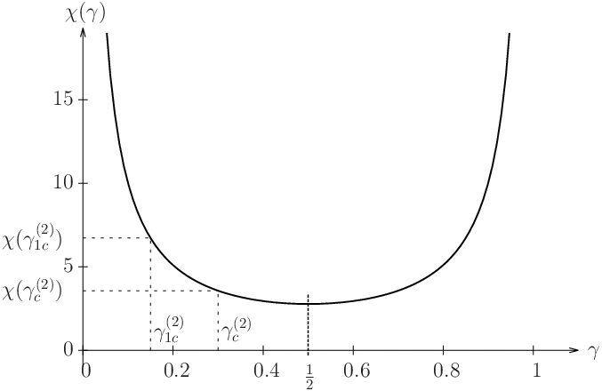
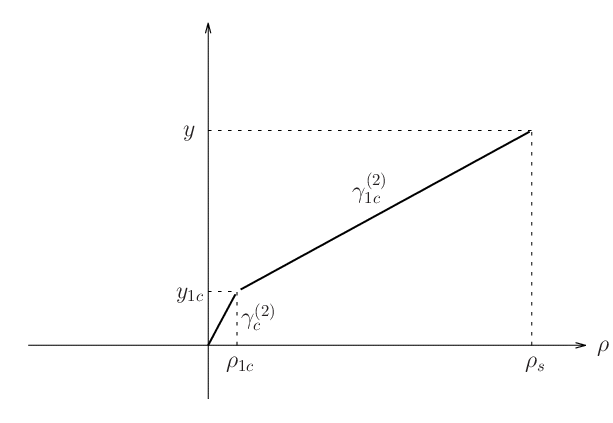
The solution in this case is represented in Fig. 3.
The solutions we have just found are qualitatively different
from what one would find in the case of a branching-diffusion process.
This question is addressed in some detail
in Appendix A.
The dipole model can be identified with
such a process when one observes the dipole density
at a fixed impact parameter, but when one integrates over the impact parameter
as we do here, then the hotspots generated by the
collinear singularities dominate, and the dipole
branching is no longer a diffusion in the logarithmic dipole sizes.
We are now going to investigate in the same spirit the higher moments of the dipole multiplicity.
5.2 Higher moments
The integral expression of the moment of order is a complicated
multiple integral of products of mean dipole numbers and densities.
For its complexity, we will not be able to study in detail
its limits in the same way as for .
Therefore, we will assume that the global saddle-point solution
essentially consists in two steps. We will see that
for large enough values of ,
the global saddle point always exists.
The first step is then the production of a larger dipole
and the second its decay into much smaller dipoles.
Let us write directly the saddle-point solution:
| (45) |
where
| (46) |
generalizes Eq. (36) taken at the saddle point, and the following relations must hold true:
| (47) |
For large , according to the first relation, necessarily . The second relation imposes . Hence one may replace the complete expression of by its collinear (resp. anticollinear ) limit whenever this function or its derivative are evaluated at (resp. ). The saddle-point equations lead to , at large . Then
| (48) |
The saddle-point solution should exist as soon as
: Hence for large enough ,
it will always be the only relevant solution.
Using this determination of the saddle-point parameters, we find . Hence the large- expression for the -th moment of the dipole number is
| (49) |
The interpretation of this solution is straightforward.
The dipoles that are measured at rapidity
stem from the evolution of a “common
ancestor”, which was produced at rapidity
(at large
). This ancestor dipole has a size which is of the order
of times bigger than the initial dipole.
We have actually just recovered the picture that was argued for in Ref. [25], where the backward step of the evolution was assumed to coincide with the very first splitting, and the further evolution was replaced by its collinear limit.
5.3 Multiplicity distribution and physical picture
From the expression of the moments of the dipole multiplicity of order in the large- limit, we can go back to the distribution using the relation (32) and replacing therein by the expression in Eq. (49). The integral to perform is Gaussian. The result reads [25]
| (50) |
The large- tail of this distribution is much fatter than
the one of the DL limit (34).
Moreover, this probability distribution does not obey KNO scaling.
If one focusses on larger multiplicities, then the evolution goes through large-size dipoles, much larger than the initial dipole. If the latter models a hadron of typical size , the production of much larger dipoles should be cut off by confinement. We shall now introduce a qualitative model for these effects, and propose a solution.
6 Evolution in the presence of confinement
Confinement is expected to act as a cutoff that prevents
dipoles of size larger
than typically to be created.
Here we are going to pick a simple model that enable us
to arrive at analytical results.
To this aim, we go back to the equation (13) for the moments of the dipole number and implement a Gaussian cutoff on the size of the produced dipoles. For technical reasons, it is convenient to use the form of the kernel in Eq. (3) and to enforce the cutoff through the substitution
| (51) |
in such a way that Eq. (13) be replaced by
| (52) |
With respect to the case without cutoff studied in the previous section, only dipoles of size less than may be created with high probability. Hence the larger span for the rapidity evolution is between the dipole sizes and . It is then natural to try an Ansatz of the form
| (53) |
for large .
We are going to check that this form is indeed an asymptotic
solution.
As in the case of , we may assume that the integral in Eq. (14) is dominated by the value of the integrand at the saddle point . Discarding the prefactors, we write
| (54) |
and solves . Looking at Eq. (52), we see that the nonlinear terms dominate the large- solution because of the -dependence of our Ansatz for . Inserting the latter into Eq. (52) deprived of the linear terms in the right-hand side, the integro-differential equation for becomes a recursion for the constants
| (55) |
which is easily simplified to
| (56) |
For large , this recursion is solved by
, where the constant
depends on on which we have no control since the linear term
we dropped in the equation (52)
for the moments plays a central role
for the moments of low .
From the large- moments, one can infer the large- behavior of the probability distribution. We find
| (57) |
Note that the value of the constant depends on the form of the recursion (56), which in turn may depend on the details of the infrared cutoff. Therefore we do not expect this constant to be universal. However, the exponential form99 9 A decreasing exponential is also the dominant behavior of the tail of the negative binomial distribution found in the glasma model, see Refs. [26, 27]. is very likely to be universal, because it requires no more than the existence of an infrared absorptive boundary in the evolution. Numerical checks would be useful in order to confirm the solution in Eq. (57) and to probe its universality.
7 Summary and outlook
In this paper, we studied the distribution of
the multiplicity of the particles produced in
high-energy onium-nucleus collisions in the forward rapidity
region of the onium,
as the simplest possible model for proton-nucleus collisions.
We investigated different kinematical regimes. First, we observed
that in the large-rapidity and small-size regime
in which the double-logarithmic (DL) approximation makes sense,
the problem formally maps to jet evolution.
We then showed that when the DL approximation is released,
the large-multiplicity distribution becomes much fatter, due
to the production of very large dipoles in the course of the
evolution. However, confinement does not allow for such
evolution paths: Once the latter are cut off, the tail of
the multiplicity distribution becomes a decreasing exponential.
The analytical results we obtained in the different regimes of
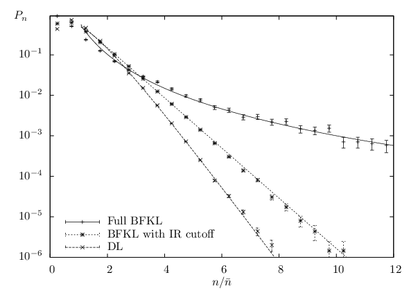
the dipole evolution are shown in Fig. 4
and compared to Monte Carlo simulations of a simple one-dimensional toy model
described in Appendix B.
A natural extension of this work would be to try and build a more realistic model for proton-nucleus collisions beyond the dipole model, in order to allow for sensible comparisons with LHC experimental data. From a more theoretical perspective, if our assumption on the relation between event-by-event partonic fluctuations in the initial state and final-state multiplicity fluctuations is correct, then the tails of the multiplicity distribution stem from dense states of gluons present in the wavefunction of the initially dilute projectile (the onium, or the proton). Understanding these rare events may open a new window on very high-density quantum states.
Acknowledgments
We acknowledge support from the France-US binational exchange program PICS, project title: “Fundamental properties of quantum chromodynamics at high energy and high density and applications at the LHC”. T.L. benefited from a Doctoral Mobility Grant awarded by the Direction des Relations Internationales of École Polytechnique at the time when this project was initiated. A.H.M. acknowledges support from the Office of Science of the U.S. Department of Energy, Grant No. DE-FG02-92ER40699. We thank Dr. Cyrille Marquet for suggesting references.
Appendix A Dipole pair multiplicity in a branching-diffusion model
In this appendix, we shall assume that is a second-order polynomial:
| (58) |
where and , , and
are constants. We assume that for all .
Such a second-order polynomial in represents
the eigenvalues of a branching-diffusion kernel
with a drift.
The technical advantage of such a diffusive model is that the
integrations over the sizes being Gaussian, they can be performed exactly.
If , , and ,
this is plain branching Brownian motion.
(For a detailed numerical and analytical study of the pair multiplicity in
the branching Brownian motion, see Ref. [28]).
If instead the constants , and
coincide with the values of the functions
,
and respectively
evaluated at ,
with ,
then Eq. (58) defines the so-called diffusive approximation
to the BFKL kernel, which has been studied in QCD.
The associated stochastic process is a branching random walk
with a drift.
The diffusive approximation to dipole branching
would be relevant if one were interested in
studying the dipole pair number at a given impact parameter
instead of integrating over all impact parameters, as we do in this paper
since the observable we consider here requires it.
Physically, if the dipole branching process
is diffusive, then the excursions
through very large dipole sizes during evolution
are highly improbable.
Let us rewrite the function in the convenient form , where
| (59) |
With such a kernel, the mean unintegrated dipole density is a Gaussian in logarithmic dipole sizes
| (60) |
where we introduced
| (61) |
This formula shows very clearly that viewed from the lines of constant
, our process is a branching diffusion with
branching rate (per unit ) and
diffusion coefficient .
At variance with BFKL, the branching and the diffusion decouple completely
in this class of models.
The mean density of pairs of dipoles of equal size reads
| (62) |
The integration is just a Gaussian integration. We are left with
| (63) |
We are going to study the large- limit of .
There are two interesting cases defined by
the relative values of
and .
Whenever is much smaller than , the integral over is dominated by a region near its lower bound. Indeed, we observe that we can write
| (64) |
The argument of the exponential is negative when . The fixed- and large- expansion of reads
| (65) |
In this regime, the “common ancestor” of the pair of
dipoles lives at the very beginning of the rapidity
evolution, typically within units of
from the start.
The picture is similar to BFKL either in the DL approximation,
or with a cutoff modeling confinement.
In the opposite regime, that is when , we write
| (66) |
where we defined . Thus
| (67) |
In this regime, since the low- region (i.e.
in terms of the initial integration variable, )
dominates
the integral in Eq. (66), the evolution is essentially
a single path until the very last splittings.
We see that there is no regime in which a large object can be produced at the beginning of the evolution, unlike in the plain BFKL case. This is due to the lack of singularities in the branching-diffusion kernel. Therefore, the diffusive approximation lacks some fundamental features of the BFKL evolution, and should be used with great care when one is interested in the integrated gluon density.1010 10 The diffusive approximation is however well-justified for the evolution of the gluon density at a fixed impact parameter, as was previously documented (see e.g. Ref. [29, 30]).
Appendix B Numerical simulations in a simplified model
In order to test qualitatively the analytical results obtained in this paper,
we perform a Monte Carlo simulation of a model that has the main features of the
color dipole model, but that is simpler and more manageable numerically.
The model we consider is a simplified version of the color dipole model.
The transverse space has only one dimension, and the evolution kernel
is reduced to the collinear and anticollinear logarithmic
singularities.
Let us introduce the logarithmic variable1111 11 Note that with the full two-dimensional transverse space, the natural variable is . to characterize a dipole of generic size . The equivalent BFKL kernel, that is the rate of splitting of a dipole of (log)size to a dipole of (log)size , reads
| (68) |
The parent dipole remains unchanged.
The equivalent BK equation for this model reads
| (69) |
The eigenfunctions of the kernel are , and the characteristic function is
| (70) |
One gets the double-log limit by simply turning off the splittings to larger dipoles
(namely by leaving out the second term in the probability
density in Eq. (68).)
On the other hand, the infrared cutoff that models confinement
is implemented by simply removing dipoles created with
a size larger than some given size of the same order as the size
of the initial dipole.
We run the Monte Carlo event generator starting from a single dipole in the three configurations we study in this paper: full BFKL, BFKL with an infrared cutoff, and DL limit. We compare the numerical results to the analytical formulae (50), (57) and (34). More precisely, we use the following parametrizations:
| (71) |
The plot in Fig. 4 shows the numerical result for the following parameters: and . The fits are performed for all numerical data points in the range . We see that the matching with the analytical formulae is very good, except, unsurprisingly, for small values of (). Since full BFKL does not obey KNO scaling, the value of is needed in that case: We take it as an output of the Monte Carlo, . We get the following determination of the parameters:
- •
BFKL: ,
- •
DL: ,
- •
BFKL with a cutoff: , .
The unnaturally large value of the normalization in the case
of the BFKL fit is due to the fact that we have neglected
potentially large but slowly varying
factors in the argument of the exponential (see Eq. (50)),
of the form .
We have not been able to test numerically the universality of and the dependence of the prefactor in the BFKL case upon the dipole size. This would require the use of a Monte Carlo that includes the full QCD dynamics, such as the one developed in Ref. [31], and to run it in a large enough range of values of and .
References
- [1] F. Gelis and B. Schenke, to appear in Annual Reviews of Nuclear and Particle Science, arXiv:1604.00335 [hep-ph].
- [2] B. Alver, M. Baker, C. Loizides and P. Steinberg, arXiv:0805.4411 [nucl-ex].
- [3] L. McLerran and M. Praszalowicz, Annals Phys. 372, 215 (2016) doi:10.1016/j.aop.2016.05.010 [arXiv:1507.05976 [hep-ph]].
- [4] A. Dumitru, E. Iancu, L. Portugal, G. Soyez and D. N. Triantafyllopoulos, JHEP 0708, 062 (2007) doi:10.1088/1126-6708/2007/08/062 [arXiv:0706.2540 [hep-ph]].
- [5] F. Gelis, R. B. Peschanski, G. Soyez and L. Schoeffel, Phys. Lett. B 647, 376 (2007) doi:10.1016/j.physletb.2007.01.055 [hep-ph/0610435].
- [6] H. Mäntysaari and B. Schenke, Phys. Rev. Lett. 117 (2016) 052301, doi:10.1103/PhysRevLett.117.052301
- [7] J. P. Blaizot, private communication.
- [8] L. N. Lipatov, Sov. J. Nucl. Phys. 23, 338 (1976) [Yad. Fiz. 23, 642 (1976)].
- [9] E. A. Kuraev, L. N. Lipatov and V. S. Fadin, Sov. Phys. JETP 45, 199 (1977) [Zh. Eksp. Teor. Fiz. 72, 377 (1977)].
- [10] I. I. Balitsky and L. N. Lipatov, Sov. J. Nucl. Phys. 28, 822 (1978) [Yad. Fiz. 28, 1597 (1978)].
- [11] A. H. Mueller, Nucl. Phys. B 415, 373 (1994).
- [12] A. H. Mueller, “Multiplicity Fluctuations in Proton Nucleus Collisions”, communication at the workshop “Ab Initio Approaches in many-body QCD confront Heavy-Ion Experiments”, Heidelberg, December 15, 2014, unpublished.
- [13] E. Iancu, A. H. Mueller and S. Munier, Phys. Lett. B 606, 342 (2005) doi:10.1016/j.physletb.2004.12.009 [hep-ph/0410018].
- [14] A. H. Mueller and S. Munier, Phys. Lett. B 737, 303 (2014) doi:10.1016/j.physletb.2014.08.058 [arXiv:1405.3131 [hep-ph]].
- [15] S. Munier, Phys. Rept. 473, 1 (2009) doi:10.1016/j.physrep.2009.02.001 [arXiv:0901.2823 [hep-ph]].
- [16] S. Munier, Sci. China Phys. Mech. Astron. 58, no. 8, 81001 (2015) doi:10.1007/s11433-015-5666-7 [arXiv:1410.6478 [hep-ph]].
- [17] Y. V. Kovchegov and E. Levin, “Quantum chromodynamics at high energy,” Cambridge Monographs on Particle Physics, Nuclear Physics and Cosmology, Cambridge University Press, 2012.
- [18] Y. V. Kovchegov and A. H. Mueller, Nucl. Phys. B 529, 451 (1998) doi:10.1016/S0550-3213(98)00384-8 [hep-ph/9802440].
- [19] A. H. Mueller, arXiv:1607.05623 [hep-ph].
- [20] I. Balitsky, Nucl. Phys. B463 (1996) 99–160.
- [21] Y. V. Kovchegov, Phys. Rev. D60 (1999) 034008.
- [22] Y. L. Dokshitzer, V. S. Fadin and V. A. Khoze, Z. Phys. C 18, 37 (1983).
- [23] Y. L. Dokshitzer, V. A. Khoze, A. H. Mueller and S. I. Troian, “Basics of perturbative QCD,” Gif-sur-Yvette, France: Ed. Frontieres (1991) 274 p.
- [24] Z. Koba, H. B. Nielsen and P. Olesen, Nucl. Phys. B 40, 317 (1972). doi:10.1016/0550-3213(72)90551-2
- [25] G. P. Salam, Nucl. Phys. B 449, 589 (1995) [hep-ph/9504284].
- [26] T. Lappi and L. McLerran, Nucl. Phys. A 772, 200 (2006) doi:10.1016/j.nuclphysa.2006.04.001 [hep-ph/0602189].
- [27] F. Gelis, T. Lappi and L. McLerran, Nucl. Phys. A 828 (2009) 149 doi:10.1016/j.nuclphysa.2009.07.004 [arXiv:0905.3234 [hep-ph]].
- [28] A. Doche, Master’s thesis report, École polytechnique, 2013.
- [29] S. Munier, G. P. Salam and G. Soyez, Phys. Rev. D 78, 054009 (2008) doi:10.1103/PhysRevD.78.054009 [arXiv:0807.2870 [hep-ph]].
- [30] A. H. Mueller and S. Munier, Phys. Rev. D 81, 105014 (2010) doi:10.1103/PhysRevD.81.105014 [arXiv:1002.4575 [hep-ph]].
- [31] G. P. Salam, Comput. Phys. Commun. 105, 62 (1997) doi:10.1016/S0010-4655(97)00066-0 [hep-ph/9601220].