Instrumental variables estimation of exposure effects on a time-to-event response using structural cumulative survival models
Torben Martinussen
Department of Biostatistics
University of Copenhagen
Øster Farimagsgade 5B, 1014 Copenhagen K, Denmark
email: tma@sund.ku.dk
Stijn Vansteelandt
Department of Applied Mathematics, Computer Science and Statistics
Ghent University
Krijgslaan 281, S9, B-9000 Gent, Belgium
email: stijn.vansteelandt@ugent.be
Eric J. Tchetgen Tchetgen
Department of Biostatistics and Epidemiology
Harvard School of Public Health
677 Huntington Avenue Kresge, Room 822
Boston, Massachusetts 02115, US
email: etchetge@hsph.harvard.edu
David M. Zucker
Department of Statistics
Hebrew University
Mount Scopus, 91905 Jerusalem, Israel
email: david.zucker@mail.huji.ac.il
Summary
The use of instrumental variables for estimating the effect of an exposure on an outcome is popular in econometrics, and increasingly so in epidemiology. This increasing popularity may be attributed to the natural occurrence of instrumental variables in observational studies that incorporate elements of randomization, either by design or by nature (e.g., random inheritance of genes). Instrumental variables estimation of exposure effects is well established for continuous outcomes and to some extent for binary outcomes. It is, however, largely lacking for time-to-event outcomes because of complications due to censoring and survivorship bias. In this paper, we make a novel proposal under a class of structural cumulative survival models which parameterize time-varying effects of a point exposure directly on the scale of the survival function; these models are essentially equivalent with a semi-parametric variant of the instrumental variables additive hazards model. We propose a class of recursive instrumental variable estimators for these exposure effects, and derive their large sample properties along with inferential tools. We examine the performance of the proposed method in simulation studies and illustrate it in a Mendelian randomization study to evaluate the effect of diabetes on mortality using data from the Health and Retirement Study. We further use the proposed method to investigate potential benefit from breast cancer screening on subsequent breast cancer mortality based on the HIP-study.
Keywords: Causal effect; confounding; current treatment interaction; G-estimation; instrumental variable; Mendelian randomization.
1 Introduction
A key concern in most analyses of observational studies is whether sufficient and appropriate adjustment was made for confounding of the association between the considered exposure of interest and outcome. This concern can be mitigated to some extent when data are available on an instrumental variable. This is a variable which is (a) associated with the exposure, (b) has no direct effect on the outcome other than through the exposure, and (c) whose association with the outcome is not confounded by unmeasured variables (see e.g. Hernán and Robins, 2006). Condition (a) is empirically verifiable, but conditions (b) and (c) are not. However, condition (c) can sometimes be justified in observational studies that incorporate elements of randomization, either by design or by nature (Didelez and Sheehan, 2007). The plausibility of condition (b) can sometimes be argued on the basis of design elements (e.g. blinding) or a priori contextual knowledge.
Instrumental variables have a long tradition in econometrics (e.g., Angrist and Krueger, 2001). They have recently become increasingly popular in epidemiology due to a revival of Mendelian randomization studies (Katan, 1986; Davey-Smith and Ebrahim, 2003). Such studies focus on modifiable exposures known to be affected by certain genetic variants. They then adopt the notion that an association between these genetic variants and the outcome of interest (e.g., all-cause mortality) can only be explained by an effect of the exposure on the outcome. This reasoning presupposes that the genetic variants studied satisfy the aforementioned instrumental variable conditions (Didelez and Sheehan, 2007). That is, they should have no effect on the outcome (e.g., all-cause mortality) other than by modifying the exposure, which can sometimes be justified based on a biological understanding of the functional genetic mechanism. Moreover, their association with the outcome should be unconfounded, which is sometimes realistic because of Mendelian randomization: the fact that genes are transferred randomly from parents to their offspring.
Instrumental variables estimation of exposure effects is well established for continuous outcomes that obey linear models. Two-stage least squares (2SLS) estimation proceeds via two ordinary least squares regressions: regressing the exposure variable on the instrument in the first stage, and next regressing the outcome variable on the predicted exposure value in the second stage. This approach presumes that the additive exposure effect is the same at all levels of the unmeasured confounders (Hernan and Robins, 2006), which is rarely plausible in the analysis of event times. The IV-analysis of event times is further complicated because of censoring and the fact that the instrumental variables assumptions, even when valid for the initial study population, are typically violated within the risk sets composed of subjects who survive up to a given time. Progress is often made via heuristic adaptations of 2SLS estimation, whereby the second stage regression is substituted by a Cox regression (see Tchetgen Tchetgen et al. (2015), and Rassen et al. (2008), Cai et al. (2011) for related approaches for dichotomous outcomes), but these have no formal justification outside the limited context of rare events (Tchetgen Tchetgen et al., 2015).
To the best of our knowledge, the first formal IV-approach for the analysis of event times was described in Robins and Tsiatis (1991), who parameterised the exposure effect under a structural accelerated failure time model and developed G-estimation methods for it. Their development is very general, and, in particular, can handle continuous exposures. However, recurring problems in applications have been the difficulty in finding solutions to the estimating equations and obtaining estimators with good precision. This is related to the use of an artificial censoring procedure, where some subjects with observed event times are made censored in the analysis in order to maintain unbiased estimating equations. This procedure may lead to an enormous information loss. Moreover, it leads to non-smooth estimating equations (Joffe et al., 2012), so that even simple models are difficult to fit. Loeys, Goetghebeur and Vandebosch (2005) proposed an alternative approach based on structural proportional hazards models. Their development does not require the use of recensoring, but is more parametric than that of Robins and Tsiatis (1991) as it requires modeling the exposure distribution. It is moreover limited to settings with a binary instrument and constant exposure at one level of the instrument, which is characteristic of placebo-controlled randomized experiments without contamination. Cuzick et al. (2007) relax this limitation by adopting a principal stratification approach but, like other such approaches (see e.g. Abadie, 2003; Nie, Cheng and Small, 2011), restrict their development to binary exposure and instrumental variables. More recently, Tchetgen Tchetgen et al. (2015) independently demonstrated the validity of two-stage estimation approaches in additive hazard models for event times when the exposure obeys a particular location shift model (see Li, Fine and Brookhart (2015) for a related approach under a more restrictive model; other related approaches are discussed in Tchetgen Tchetgen et al., 2015). In this article, we avoid restrictions on the exposure distribution and develop IV-estimators under a semiparametric structural cumulative survival model that is closely related to, but less restrictive than the additive hazard model in Tchetgen Tchetgen et al. (2015) and Li, Fine and Brookhart (2015). The proposed approach is general in that it can handle arbitrary exposures and instrumental variables, and can accommodate adjustment for baseline covariates. It neither requires modelling the exposure distribution nor the association between covariates and outcome, and it naturally deals with administrative censoring and certain forms of dependent censoring. Picciotto et al. (2012) studied the different problem of adjusting for time-varying confounding when estimating the effect of a time-varying exposure on a survival outcome. While we also make use of the structural cumulative failure time model, we do this for handling the different problem of estimating the effect of an exposure on a survival outcome in the presence of unobserved confounding using an instrumental variable. Because of this and the fact that we make use of semi-parametric continuous-time models, in contrast to Picciotto et al. (2012) who focus on parametric discrete-time models, the recursive estimators that we propose cannot be immediately compared with those in Picciotto et al. (2012). A further strength of our paper is that it develops an asymptotic inference for the proposed recursive estimators; such theory is currently lacking for G-estimators in structural cumulative failure time models. The semiparametric estimator that we propose requires only a correct model for the conditional mean of the instrumental variable, given covariates, for consistency of the estimated causal effect. Besides deriving its large sample properties we also develop inferential tools allowing us for instance to investigate for time-changing exposure effect. We examine the performance of the proposed method in simulation studies and two empirical studies.
2 Model specification and estimation
2.1 Basics
Our goal is to estimate the effect of an arbitrary exposure on an event time under the assumption that is an instrumental variable, conditional on a covariate set . A data-generating mechanism that satisfies this assumption is depicted in the causal diagram (Pearl, 2009) of Figure 1. Here, the instrumental variables assumptions are guaranteed by the absence of a direct effect of on , and by the absence of effects of the unmeasured confounder on , and of on .
To provide insight, we will start by considering uncensored survival data under the following semi-parametric variant of the additive hazards model (Aalen, 1980):
| (1) |
where denotes the counting process, the history spanned by , is the at risk indicator, is an unknown, non-negative function of time, and , and is an unknown scalar at each time . Note that the righthand side of this model does not involve because of the instrumental variables assumptions, which imply that and are conditionally independent, given and . Note furthermore that we explicitly choose to leave unspecified because is unmeasured, thus making assumptions about the hazard’s dependence on rather delicate.
Under model (1),
| (2) |
which captures the exposure effect of interest by virtue of conditioning on the unmeasured confounder . By the collapsibility of the relative risk (or the related collapsibility of the hazard difference (Martinussen and Vansteelandt, 2013)), this is also equal to the directly standardized relative survival risk:
where the averaging is over the conditional distribution of given . Letting , for each fixed , denote the potential outcome that would have been observed if the exposure were set to by some intervention, this can also be written as
| (3) |
This can be seen because, by definition of being sufficient to adjust for confounding of the effect of on , we have that is conditionally independent of , given .
That the effect can also be defined without making reference to the unmeasured confounder (that is, without conditioning on ) is important. Indeed, the lack of data on as well as the lack of a precise understanding of the variables contained inside , would otherwise make interpretation difficult (Vansteelandt et al., 2011).
Model (1) is closely related to the structural cumulative survival model:
| (4) |
This model is slightly less restrictive than model (1). It makes no assumptions as to how the unmeasured confounders are associated with the event time. It moreover models the effect of setting the exposure to zero, within exposure subgroups rather than the entire population. By evaluating effects within exposure subgroups, the parameter in model (4) thus encodes a type of treatment effect in the treated. Under the additional assumption that there is no current treatment interaction (Hernán and Robins, 2006), a population-averaged interpretation can be made. In particular, suppose that within levels of and , the effect of exposure level versus 0 on the survival function is the same for subjects with observed exposure as for subjects with a different exposure level in the following sense
| (5) |
Then it is easily verified that, as is the case for model (1), model (4) along with the assumption of no current treatment interaction implies (3), so that captures a population-averaged effect.
Under the instrumental variables assumptions that and are associated, conditional on , and that is conditionally independent of , given , the estimators of that we will propose in the next section will be consistent estimators of in both models (1) and (4). Condition (5) is not required for the estimation methods that we develop later on; it is only needed to provide the population-level interpretation given in (3).
2.2 Estimation
We will allow for the event time to be subject to right-censoring. In that case, we only observe whether or not exceeds a random censoring time , i.e. we observe , along with the first time either failure or censoring occurs, i.e. we also observe . Let , denote independent identically distributed replicates under the structural cumulative failure time model (1) together with the instrumental variables assumptions. It is assumed that and are independent given and that . In fact, the above condition on the censoring distribution can be relaxed to for some variable . The counting processes , are observed in the time interval , where is some finite time point. Further, we define the at risk indicator , .
The crux of our estimation method for is that once the exposure effect has been eliminated from the event time, it only retains a dependence on and . It thus becomes conditionally independent of the instrumental variable, given . In particular, using arguments similar to those of Martinussen et al. (2011), we eliminate the exposure effect from the increments by calculating , as suggested by (1), and we will eliminate the exposure effect from the at risk indicators by calculating , as suggested by (2). It follows that
| (6) |
for each , which can be seen formally as follows
here, the last equality follows because .
The unbiasedness of equation (6) suggests a way of estimating the increments by solving equation (6) for each with population expectations replaced by sample analogs. This delivers the recursive estimator defined by
| (7) |
where , with a parametric model for and a consistent estimator of (e.g., a maximum likelihood estimator).
The estimator (7) is given by a counting process integral, thus only changing values at observed death times. Because of its recursive structure, we calculate it forward in time, starting from . In the special case where the exposure is binary, it can be calculated analytically as shown below. With , the equation (6) (with population expectations substituted by sample averages) leads to
When replacing with on the right side of this expression and integrating, we get the Volterra equation (see Andersen et al. (1993), p. 91)
where
and the solution is given by
With the additional assumption that , that is assuming a time-constant effect, an estimator of may be obtained as
| (8) |
with , .
3 Large sample results
The following proposition, whose proof is given in the Appendix, shows that is a uniformly consistent estimator of . It moreover gives the asymptotic distribution of .
Proposition 1
Under model (4) with the assumption that is an instrumental variable, conditional on , and given the technical conditions listed in the Appendix, the IV estimator is a uniformly consistent estimator of . Furthermore, converges in distribution to a zero-mean Gaussian process with variance . A uniformly consistent estimator of is given below.
Let be the iid zero-mean processes given by expression (27) in the Appendix. From the proof in the Appendix, it then follows that is asymptotically equivalent to . The variance of the limit distribution can thus be consistently estimated by
where is obtained from by replacing unknown quantities with their empirical counterparts. These results can be used to construct a pointwise confidence band. The asymptotic behavior of the estimator (8) is easily obtained since:
To study temporal changes, it is more useful to consider a uniform confidence band. This and tests of the hypothesis of a linear (cumulative) causal effect
can easily be derived based on the above iid representation as also outlined in Martinussen (2010). The above hypothesis can be tested using the following test statistic
| (9) |
and since, under the null, it is easy to get the iid-representation of the test process. This development is based on the following approach of Lin et al. (1993). Let be independent standard normal variates. Then, given the data,
also converges in distribution to a zero-mean Gaussian process with variance . The limit distribution can thus be evaluated by generating a large number, , of replicates , . The causal null hypothesis that for all can thus for example be tested using the test statistic
by investigating how extreme this statistic is in the distribution of , .
4 Numerical results
4.1 Simulation study
To investigate the properties of our proposed methods with practical sample sizes, we conducted a simulation study. We generated data according to the data-generating mechanism of Figure 1 with the following specific models where we leave out the covariate for simplicity. We considered two different settings where the exposure variable was continuous and binary, respectively. In the first setting the exposure variable was continuous. We took to be binary with , and generated and , given , from a normal distribution with , and with variance-covariance matrix so that , and . The parameter determines the size of the correlation between exposure and the instrumental variable. Specifically we looked at correlation equal to 0.3 and 0.5. We generated according to the hazard model
with , and . Twenty percent were potentially censored according to a uniform distribution on (0,3.5), and the rest were censored at , corresponding to the study being closed at this time point, leading to an cumulative censoring rate of around 20. Under this model, as seen in the Section 2.2, (4) holds with . Under this model it further holds that
with so the naive Aalen estimator (using and as covariates) is biased. We calculated the estimator given in (7) with , along with the estimator given in (9) where we took . For this scenario, we considered sample sizes 1600 and 3200 when , and sample sizes 800 and 1600 when . Simulation results concerning , based on 2000 runs for each configuration, are given in Table 1, where (average) biases are reported at time points for along with coverage probability of 95% pointwise confidence intervals CP(). Results concerning are given in Table 3, first half.
Table 1 about here
| n | n | |||||||
|---|---|---|---|---|---|---|---|---|
| Bias | 1600 | -0.003 | -0.001 | -0.007 | 800 | -0.002 | -0.004 | - 0.015 |
| sd () | 0.139 | 0.242 | 0.404 | 0.109 | 0.187 | 0.303 | ||
| see () | 0.139 | 0.245 | 0.439 | 0.107 | 0.187 | 0.314 | ||
| 95% CP() | 95.4 | 96.5 | 98.1 | 95.2 | 96.1 | 97.5 | ||
| Bias | -0.101 | -0.201 | -0.300 | -0.099 | -0.197 | - 0.297 | ||
| Bias | 3200 | -0.003 | -0.005 | -0.014 | 1600 | 0.004 | 0.004 | -0.002 |
| sd () | 0.094 | 0.170 | 0.267 | 0.075 | 0.131 | 0.209 | ||
| see () | 0.096 | 0.166 | 0.262 | 0.075 | 0.130 | 0.206 | ||
| 95% CP() | 95.6 | 95.1 | 96.2 | 95.0 | 95.5 | 95.7 | ||
| Bias | -0.099 | -0.200 | -0.296 | -0.099 | -0.200 | -0.301 | ||
| n | n | |||||||
|---|---|---|---|---|---|---|---|---|
| Bias | 1600 | 0.005 | 0.008 | 0.001 | 800 | -0.001 | 0.001 | - 0.006 |
| sd () | 0.136 | 0.224 | 0.336 | 0.108 | 0.176 | 0.249 | ||
| see () | 0.138 | 0.228 | 0.363 | 0.107 | 0.176 | 0.264 | ||
| 95% CP() | 96.2 | 96.2 | 96.5 | 95.2 | 96.0 | 97.1 | ||
| Bias | 3200 | 0.003 | -0.001 | -0.004 | 1600 | 0.001 | 0.005 | 0.003 |
| sd () | 0.097 | 0.156 | 0.224 | 0.076 | 0.122 | 0.175 | ||
| see () | 0.096 | 0.157 | 0.230 | 0.075 | 0.121 | 0.173 | ||
| 95% CP() | 95.1 | 95.4 | 96.6 | 94.8 | 95.0 | 95.5 | ||
In all scenarios considered the naive Aalen estimator is, as expected, biased; see Table 1. From Table 1 it is also seen that the proposed estimator is unbiased. In the case with sample size 800 and correlation equal to 0.3 the estimated standard error at time point is a bit too large resulting in a too high coverage probability. However, it is also seen that the estimated standard error approaches the empirical standard deviation as sample size goes up, and overall the 95%-coverage probabilities have the correct size. We also calculated the size of the sup-test (9) that investigates whether the constant exposure effects model is acceptable. For the four considered scenarios of : (1600,0.3), (3200,0.3), (800,0.5), (1600,0.5), it was 0.03, 0.04, 0.03 and 0.05, respectively. Hence, when sample size and correlation goes up, the test has the correct size. The results concerning the constant effect estimator, , are reported in the first half of Table 4, and from there it is seen that the estimator is unbiased and that the variability is well estimated leading to satisfactory coverage probabilities at least when sample size goes up. When the exposure is continuous one may also calculate the 2SLS estimator of Tchetgen et al. (2015), we denote it . Results for this estimator are also given in Table 4. From there it is seen that this estimator is also unbiased, and that it is sligtly more efficient than the constant effects estimator given in this paper. This is not surprising as the 2SLS estimator is targeted at this specific situation while the estimator is derived from an estimator that can handle much more general situations. We also considered a setup where there was a time-varying exposure effect. Data was generated as described above except that was now taken as . Inducing censoring as above resulted in a cumulative censoring rate of around 25. Results from this study are given in Table 2, where we have dropped results for the naive Aalen estimator. From Table 2 we see again that the proposed estimator is unbiased and that the variability is well estimated resulting in appropriate coverage. We also calculated the size of the sup-test. For the four considered scenarios of : (1600,0.3), (3200,0.3), (800,0.5), (1600,0.5), it was 0.07, 0.18, 0.13 and 0.31, respectively. We also ran the situation where and obtained the size of the test to be 0.61. Whe thus see, as expected, that when correlation and sample size goes up the power of the test increases. We also calculated the constant effects estimators and , and the mean of them in all four combinations of was 0.04 thus showing that the constant effects estimators are not appropriate under this scenario with time-changing exposure effect.
We also considered settings where the exposure variable was binary. In the first such setting we generated data as under the first scenario with , but instead of using the continuous version of , call it now , we used .
Table 2 about here
We used the same censoring mechanism and also the same hazards model as under the first setting. For this scenario, we considered sample sizes 3200 and 6400 when , and sample sizes 1600 and 3200 when . Results, again based on 2000 runs for each configuration, are shown in Table 3. For the case the coverage probability is a bit too high at . In the other settings the estimator is unbiased and coverage is satisfactory. The results concerning the constant effect estimator, , are reported in the second half of Table 4, and from there it is seen that the estimator is unbiased and that the variability is well estimated leading to satisfactory coverage probabilities. We also see that 2SLS estimator of Tchetgen et al. (2015) seems to be unbiased in this setting although there is no theoretical underpinning of this. To look further into this and to stress that the 2SLS estimation relies on a correct specification of a model for the exposure given the instrument we ran a final study as follows. The instrument was taken to be normally distributed with mean 2 and variance . The unobserved was taken to be with generated as normal with mean 1 and variance . The exposure was binary with
In this way the correlation between and was approximately 0.56. We generated according to the hazard model
and censored all at resulting in approximately 25% censorings. We used sample size and with 1000 runs for each configuration. We calculated the 2SLS estimator in two ways using different first stage models; we denote the 2SLS estimator based on regressing on (despite that is binary) in the first stage by and the 2SLS estimator based on a first stage logistic regression model using as explanatory variable by . We stress that the estimator suggested in this paper, , is not based on any modelling of given in contrast to the 2SLS estimator. Results are given in Table 5 where it is seen that the estimator is unbiased while the two versions of the 2SLS estimator are both biased.
| n | n | |||||||
|---|---|---|---|---|---|---|---|---|
| Bias | 3200 | 0.000 | 0.001 | -0.017 | 1600 | -0.000 | -0.005 | -0.022 |
| sd () | 0.109 | 0.194 | 0.316 | 0.102 | 0.183 | 0.306 | ||
| see () | 0.109 | 0.194 | 0.331 | 0.102 | 0.183 | 0.302 | ||
| 95% CP() | 95.3 | 95.4 | 96.6 | 95.7 | 95.6 | 96.1 | ||
| Bias | -0.082 | -0.164 | -0.248 | -0.085 | -0.167 | - 0.249 | ||
| Bias | 6400 | -0.000 | -0.006 | -0.015 | 3200 | 0.001 | 0.001 | -0.005 |
| sd () | 0.077 | 0.137 | 0.221 | 0.071 | 0.128 | 0.202 | ||
| see () | 0.077 | 0.135 | 0.216 | 0.072 | 0.128 | 0.207 | ||
| 95% CP() | 95.1 | 94.6 | 95.2 | 95.1 | 95.2 | 95.9 | ||
| Bias | -0.082 | -0.167 | -0.250 | -0.083 | -0.168 | -0.253 | ||
| Continuous | ||||
|---|---|---|---|---|
| (1600,0.3) | (3200,0.3) | (800,0.5) | (1600,0.5) | |
| Bias | -0.002 | -0.004 | -0.003 | 0.001 |
| sd () | 0.107 | 0.074 | 0.082 | 0.057 |
| see () | 0.113 | 0.073 | 0.084 | 0.057 |
| 95% CP() | 97.2 | 95.5 | 96.1 | 95.5 |
| Bias | 0.003 | -0.001 | -0.003 | 0.001 |
| sd () | 0.098 | 0.068 | 0.075 | 0.053 |
| Binary | ||||
| (3200,0.3) | (6400,0.3) | (1600,0.5) | (3200,0.5) | |
| Bias | -0.002 | -0.004 | -0.003 | -0.000 |
| sd () | 0.085 | 0.061 | 0.082 | 0.056 |
| see () | 0.088 | 0.062 | 0.081 | 0.057 |
| 95% CP() | 96.2 | 95.4 | 95.5 | 95.4 |
| Bias | 0.001 | -0.001 | -0.001 | -0.002 |
| sd () | 0.072 | 0.050 | 0.068 | 0.048 |
| n | mean | sd () | mean | sd () | mean | sd () |
|---|---|---|---|---|---|---|
| 1000 | -0.002 | 0.117 | 0.069 | 0.117 | 0.039 | 0.100 |
| 2000 | -0.002 | 0.079 | 0.067 | 0.079 | 0.038 | 0.068 |
4.2 Application to the HRS on causal association between diabetes and mortality
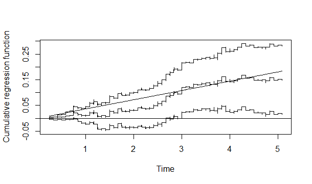
We illustrate the proposed method using data from the Health and Retirement Study (HRS), a cohort initiated in 1992. The same data was used by Tchetgen Tchetgen et al. (2015) (TT) to investigate the causal association between diabetes and mortality. The HRS consists of persons ages 50 years or older and their spouses. There are genotype data for 12123 participants, but, like TT, we restrict our analyses to the 8446 non-Hispanic white persons with valid self-reported diabetes status at baseline. The average follow-up time was 4.10 years with a total of 644 deaths over 34055 person-years. We used an externally validated genetic risk score predictor of type 2 diabetes as IV. The risk score is based on 39 SNPs that were strongly associated with the diabetes status, Likelihood ratio test chi-square statistic equal to 176.75 with 39 degrees of freedom, p-value < . Like TT we used as observed confounders () age, sex and the top 4 genomewide principal components to account for possible population stratification. The 2SLS control function approach used in TT is only valid if the instrument is binary unless one makes a further linearity assumption concerning a conditional mean of the un-observed confounder(s), specifically they assume that is linear in . This assumption is un-testable based on the observed data. The method we suggest in this paper is not restricted to only binary instruments. As a matter of fact no restrictions are put on neither the exposure nor the instrument. They can be binary as well as continuous. Also, the approach taken in TT assumes a time-constant exposure effect whereas the approach suggested in this paper allows the exposure effect to vary with time, and we may test whether a time-constant seems reasonable. The analysis used here thus generalizes that of TT in several aspects. Figure 2 shows the estimated causal effect of diabetes status on mortality, , along with 95% pointwise confidence bands. The straight line corresponds to the constant effects estimator (8). From Figure 2 it seems reasonable to assume a time-constant exposure effect, which we can formally test using the statistic (9). This procedure gives a p-value of 0.61 thus giving no evidence against the time-constant exposure effect model. The estimate of the time-constant exposure effect is with estimated standard error 0.0142 corresponding to the 95% confidence interval (0.008,0.064). So there seems to be a causal association between diabetes status and all cause mortality corresponding to an average of 3.6 additional deaths occurring for each year of follow-up in each 100 persons with diabetes alive at the start of the year, compared with each 100 diabetes-free persons alive at the start of the year, conditional on age and sex. This estimated effect is less than half of that obtained by TT suggesting that the linearity assumption used in TT may not hold.
4.3 Application to the HIP trial on effectiveness of screening on breast cancer mortality
The Health Insurance Plan (HIP) of Greater New York was a randomized trial of breast cancer screening that began in 1963. The purpose was to see whether screening has any effect on breast cancer mortality. About 60000 women aged 40-60 were randomized into two approximately equally sized groups. Study women were offered the screening examinations consisting of clinical examination, usually by a surgeon, and a mammography. Further three annual examinations were offered in this group. Control women continued to receive their usual medical care. About 35% of the women that were offered screening refused to participate (non-compliers), see Table 5. There were large differences between the study women who participated and those who refused (Shapiro, 1977) and therefore the results from the "as treated" analysis may be doubtful due to unobserved confounding.
| Control | Screening group | |||
|---|---|---|---|---|
| Group | ||||
| All | Compl. | Non-compl. | ||
| n | 30565 | 30130 | 20146 | 9984 |
The same data were analysed by Joffe (2001) and as he did, we will also focus on the first 10 years of follow-up. Since screening ended after three years, Joffe argued that focussing on the first 10 years of follow up will reduce attenuation of the effects of screening in the later periods in which treatment was the same both groups. We can look into the possibility of a time-varying effect in a more formal way as our estimator captures this directly. To begin with we performed a Cox-regression intention to treat analysis showing that there is reduced mortality from breast cancer in the screening group (p=0.01). We also applied the Aalen additive hazards intention to treat analysis. Figure 2 shows the estimated cumulative regression coefficient along with 95% confidence intervals indicating a time-varying effect of the screening; there seems to be a beneficial effect in the first 6 years or so, and no effect thereafter. The supremum test of an overall effect of screening is significant (p=0.005).
We will now apply our suggested method to estimate the causal effect of screening using the randomisation variable as instrument. In our notation, the randomization variable is called and the treatment, screening, is called . Before proceeding, it is important to notice that there is a competing risk issue in these data. In the first 10 years of follow-up there are 4221 deaths but only 340 were deemed due to breast cancer. The th counting process in our estimator (7) is now the counting process that jumps at time point if the th women at that point in time dies from breast cancer. We show in a separate report to be communicated elsewhere that contrasts the cumulative breast cancer death specific hazards among the treated between scenarios with versus without screening under the assumption that the cause specific hazard of death due to other causes than breast cancer for the screened women would have been the same at all times had they not been screened. To test this assumption one may use the test process
where is the th counting process counting non-breast cancer death. Under the null of no causal effect of screening on the non-breast cancer death hazards, this process is a zero-mean process. One may further show that
where are independent identically distributed zero-mean processes. Specifically,
considering here the case without covariates so that . In the previous display, and are the limits in probability of
respectively. This representation can be used to resample from the limit distribution of under the null. Further, a formal test based on for instance may be performed and whether or not it is significant can also be

based on resampling from the limit distribution under the null. Figure 3 shows the test process along with 20 resampled processes from its limit distribution under the null, and it is seen that the test process does not seem to deviate in any respect. The supremum test based on 1000 resamples results in a p-value of 0.63. Based on this, we proceed to calculate the estimator . This estimate along with 95% confidence bands (pointwise) are given in Figure 4 that also shows the intention to treat estimate (broken curve). The causal effect of the screening appears to be slightly more pronounced than what is seen from the intention to treat estimator and again it is seen that there seems to be a time-varying effect with screening being beneficial in a period of approximately 6 years. The supremum test is significant (p=0.02).
Using our approach it is now possible to study the time-dynamics even further. For illustrative purposes, let us assume that it had been hypothesized that if there were an effect of screening it would only last for a few years (as screening stopped after 3 years), and let us say it corresponds to roughly six years of follow up. We could then attempt the simpler model
| (10) |
with years. The two parameters and are estimated by
with , , . The estimate of under this simplified model is then given by
| (11) |
The constant effects parameters are estimated to (SE 0.00011) and (SE 0.00020), indicating a significant effect of the screening only in the first 6 years. The estimator is shown in Figure 4. To test whether the simplified model, that is assuming a constant effect of treatment with a change in the effect after 6 years, gives a reasonable description of the data we consider the test process which, under the null, can be written as
Using the iid representation of we can resample from the limit distribution, under the null, of ; such 20 randomly picked processes are shown in Figure 5 along with the observed test process . We may use the supremum test statistic to investigate whether the test process is deviating. To see whether the observed is extreme we sampled 1000 draws from the limit distribution as outlined in Section 3; this gave a p-value of 0.56 suggesting that the constant effects model with a change in the effect after 6 years gives a reasonable fit to the data.
However, it also seen from Fig. 4 and Fig. 5 that the two parameter constant effects model is perhaps not giving a fully satisfactory fit in the first period of follow-up (two years or so). Actually, if instead one uses the test statistic then one gets a p-value of 0.06 giving some indication of a non-satisfactory fit in the initial phase of the follow up period. One could consider extending the two parameter constant effects model with an additional parameter allowing for a separate effect in the initial phase of two years or so. The cutpoints chosen here were used for illustrative purposes only, in practice they should have been specified ahead of performing the analysis.
5 Concluding remarks
In this article, we proposed an instrumental variables estimator for the effect of an arbitrary exposure on an event time. In comparison with other instrumental variables estimators for event times, our proposed approach has the advantage that it can handle arbitrary (e.g., continuous) exposures, without the need for modelling the exposure distribution, and that it naturally adjusts for censoring whenever censoring is independent of the event time, exposure and instrument, conditional on measured and unmeasured confounders. The independent censoring assumption is relatively weak as it allows for a dependence on unmeasured factors. This assumption can be relaxed via inverse probability of censoring weighting under a model for the dependence of censoring on the exposure and/or instrumental variable.
Under the usual instrumental variable assumptions, listed in Section 1, the IV-estimator (8) provides a consistent estimator of the causal exposure effect as opposed to the naive estimator when there is unmeasured confounding. However, in the case of a weak instrument, the IV-estimator may have a large variance. It is therefore of interest to develop semi-parametric efficient estimators (Tsiatis, 2006). Along the same lines, it is also of interest to consider estimators that are robust to some model deviations. For instance, consider the following two models
| (12) |
and
| (13) |
where is a user defined function such as ; and and are parameters indexing the two models. Consider then the estimating function
| (14) |
where
and is an arbitrary index function. One may then show that (14) has zero mean if either model (12) or model (13) hold; the solution to an estimating equation based on estimating function (14) therefore yields a double robust estimator. This estimator has the further advantage of being invariant to linear transformations of the exposure. A detailed study of efficient and double robust estimators will be communicated in a separate report.
Acknowledgement
Torben Martinussen’s work is part of the Dynamical Systems Interdisciplinary Network, University of Copenhagen. Stijn Vansteelandt was supported by IAP research network grant nr. P07/05 from the Belgian government (Belgian Science Policy). Eric Tchetgen Tchetgen is supported by NIH grant R01A I104459.
Appendix: Large sample properties
Let be the conditional mean of the instrument given observed confounders , which is function of an unknown finite-dimensional parameter . In the case of no observed confounders and . We assume that , where the ’s are zero-mean iid variables. In the case of no observed confounders we have . Let denote the true value of .
We write and use the notation to denote the total variation
of over the interval .
Let denote the true value of , and let .
Technical conditions:
- (i)
We assume that and are bounded, and denote the respective bounds by and .
- (ii)
Define . We assume that there exist and such that .
The quantities and do not necessarily need to be known.
Consistency
Below we show that is uniformly consistent. In what follows we suppress from the notation and write instead of . The estimator is given by the recursion equation
| (15) |
It appears difficult to prove directly that is bounded. Instead we will take a different approach. We will modify the estimator in a way that will force it to be of bounded variation. We will then prove that the modified version of the estimator is consistent. If is not known, the modified estimator is a theoretical construct that cannot actually be computed, but it will emerge that for large enough the modified estimator is equal to the unmodified estimator.
We will use the Helly Selection Theorem in the following form.
Helly Selection Theorem: Let be a sequence of functions on such that and , where and are finite constants. Then
a. There exists a subsequence of which converges pointwise to some function .
b. If is continuous, the convergence is uniform.
Then it follows that .
Proof: For a function on , define
| (16) | ||||
| (17) |
where
| (18) | ||||
| (19) |
with , so that . The estimator is then the solution to . Let . We then define the modified estimator to be the solution to the equation . Note that .
Define , so that
The function satisfies , where is an upper bound on (which we assume exists). Moreover, is Lipschitz with respect to over and with Lipschitz constant . Accordingly, by classical differential equations theory (Hartman, 1973, Thm. 1.1; Coddington, 1989, Sec. 5.8), is the unique solution to the equation subject to .
We note for later reference that for any two functions and we have
| (20) |
Now, by the functional central limit theorem as given in Andersen and Gill (1982),
| (21) |
Accordingly, from the the assumption that , we get the result that for sufficiently large. We thus find that the jumps in are bounded by with , implying that and . Let denote the class of functions with these two properties. Further, let denote the class of functions that are bounded by and have total variation less than . Since and is Lipschitz(1), we find that implies that .
For , define
| (24) |
We then have . We claim that the class of functions is Donsker. This result is an immediate consequence of the following facts:
1. Sums and products of bounded Donsker classes are also Donsker.
2. For any finite , the class of monotone functions mapping to is Donsker (Kosorok, 2008, Thm. 9.24).
3. If is bounded and has bounded variation, then can be written as , where and are monotone increasing functions with and (Jordan decomposition). It follows that the class of functions with and is Donsker.
4. If , then the function is bounded and of bounded variation with and
where .
It follows that
| (25) |
and therefore
| (26) |
Now, by Helly’s selection theorem, every subsequence of has a further subsequence that converges to some limit. Since the jumps are bounded by and the number of jumps in the interval divided by converges uniformly to for some constant , it follows that the limit of the sub-subsequence is continuous, and therefore (by the second part of Helly’s theorem) the convergence of the sub-subsequence is uniform. Going further, the fact that in combination with (20) and (26) implies that the limit of the sub-subsequence satisfies . But we said before that is the unique continuous solution to this equation. We thus find that every subsequence of has a further subsequence that converges uniformly to . Consequently, itself converges uniformly to . Since and (as just stated), for sufficiently large we have and therefore . So for sufficiently large, solves , or, in other words . We have thus shown that , as desired.
The consistency of then follows immediately by a Taylor series expansion since is consistent.
Asymptotic normality
Let and . For known we can write
where the th element of the -vector is
Let and let denote the derivative of with respect to its second argument. It is then easy to see that
which is a Volterra-equation, see Andersen et al. (1993), p. 91. The solution to this equation is given by
where
with the latter being a product integral that converges in probability to some limit. This leads to the iid-representation
with the ’s being zero-mean iid terms. Specifically
with being the th element of the vector . This together with
where is the first order derivative of w.r.t. gives an iid-decomposition of :
where
| (27) |
We now argue that the process converges in distribution as a process using arguments similar to what is done in Lin et al. (2000. p. 726). By taking the to equation (4) it is seen that can be written as a difference of two monotone functions . Let be the limit in probability of . Now, split into its positive and negative parts, and , and similarly with , and . Then can be written as a difference of two monotone functions, and then we follow the arguments of Lin et al. (2000) (or use example 2.11.16 of van der Vaart and Wellner, 1996). Convergence in distribution for the process also holds using the above Taylor expansion. It thus follows that
converges to a zero-mean Gaussian process with a variance that is consistently estimated by
The derivative can be calculated recursively as is constant between the observed death times. Denote the jump times by . Hence
which then also holds for the derivative. Since and the derivative of the increment in the first jump time, , is easily calculated we then have a recursive way of calculating the derivatives of .
References
Aalen, O. (1976). Nonparametric Inference in Connection with Multiple Decrement Models. Scandinavian Journal of Statistics, 3, 15-27.
Aalen, O. O. (1980). A model for non-parametric regression analysis of counting processes. Lecture Notes in Statistics, 2, 1-25.
Abadie, A. (2003). Semiparametric instrumental variable estimation of treatment response models journal of Econometrics, 113, 231-263.
Andersen, P. K., and Gill, R. D. (1982). Cox’s Regression Model for Counting Processes: A Large Sample Study. Annals of Statistics, 10, 1100-1120.
Andersen, P. K., Borgan, O., Gill, R. D. and Keiding, N. (1993). Statistical Models Based on Counting Processes. Berlin: Springer-Verlag.
Angrist, J. and Imbens, G. (1991). Sources of identifying information in evaluation models. Technical Working Paper 117, National Bureau of Economic Research, Cambridge, MA.
Angrist, J. and Krueger, A. (2001). Instrumental variables and the search for identification: From supply and demand to natural experiments. Journal of Economic Perspectives 15, 69-85.
Bochud, M. and Rousson, V. (2010). Usefulness of mendelian randomization in observational epidemiology Int. J. Environ. Res. Public Health, 7, 4726-4747.
Boef, A.G. C., le Cessie, S. and Dekkers, O. M. (2015). Mendelian randomization studies in the elderly. Epidemiology, 26, e15-e16.
Burgess, S. and CRP CHD Genetics Collaboration (2013). Identifying the odds ratio estimated by a two-stage instrumental variable analysis with logistic regression model. Statistics in Medicine, 32, 711-728.
Cai, B., Small, D. S. and Ten Have, T. R. (2011). Two-stage instrumental variable methods for estimating the causal odds ratio: analysis of bias. Statistics in Medicine, 30, 1809-1824.
Clarke, P. S. and Windmeijer, F. (2010). Identification of causal effects on binary outcomes using structural mean models. Biostatistics, 11, 756-770.
Clarke, P. S. and Windmeijer, F. (2012). Instrumental variable estimators for binary outcomes. Journal of the American Statistical Association, 107, 1638-1652.
Coddington, E. A. (1989). An Introduction to Ordinary Differential Equations. Mineola: Dover
Cuzick, J., Sasieni, P., Myles, J., et al. (2007). Estimating the effect of treatment in a proportional hazards model in the presence of non-compliance and contamination. Journal of the Royal Statistical Society - Series B 69, 565-588.
Davey-Smith, G. and Ebrahim, S. (2003). Mendelian randomization’: can genetic epidemiology contribute to understanding environmental determinants of disease? International Journal of Epidemiology 32, 1-22.
Didelez, V. and Sheehan, N. (2007). Mendelian randomization as an instrumental variable approach to causal inference. Statistical Methods in Medical Research 16, 309-330.
Hartman, P. (1973). Ordinary Differential Equations, 2nd ed. (reprinted, 1982), Boston: Birkhauser.
Harbord, R. M., Didelez, V., Palmer, T. M., Meng, S., Sterne, J. A. C and Sheehan, N. A. (2012). Severity of bias of a simple estimator of the causal odds ratio in Mendelian randomization studies. Statistics in Medicine, 32, 1246-1258.
Hernán, M. A. and Robins J. M. (2006). Instruments for causal inference: an epidemiologist’s dream? Epidemiology 17, 360-372.
Imbens, G. W. and Angrist, J. (1994). Identification and estimation of local average treatment effects. Econometrica 62, 467-476.
Joffe, M.M. (2001). Administrative and artificial censoring in censored regression models. Statistics in Medicine 20, 2287-2304.
Joffe, M.M., Yang, W.P. and Feldman, H. (2012). G-Estimation and Artificial Censoring: Problems, Challenges, and Applications. Biometrics 68, 275-286.
Katan M. B. (1986) Apolipoprotein E isoforms, serum cholesterol, and cancer. Lancet 507-8.
Kosorok, M. R. (2008). Introduction to Empirical Processes and Semiparametric Inference. Berlin: Springer-Verlag.
Li, J., Fine, J. and Brookhart, A. (2014). Instrumental variable additive hazards models. Biometrics, 71, 122-130.
Lin, D. Y., Wei, L. J., Yang, I. and Ying, Z. (2000). Semiparametric regression for the mean and rate functions of recurrent events. Journal of the Royal Statistical Society - Series B, 62, 711-730.
Loeys, T., Goetghebeur, E and Vandebosch, A. (2005). Causal proportional hazards models and time-constant exposure in randomized clinical trials. Lifetime Data Analysis 11, 435-449.
Martinussen, T. (2010). Dynamic path analysis for event time data: large sample properties and inference. Lifetime Data Analysis, 16, 85-101.
Martinussen, T., Vansteelandt, S., Gerster, M. and Hjelmborg, J. V. B. (2011) Estimation of direct effects for survival data by using the Aalen additive hazards model. Journal of the Royal Statistical Society - Series B, 73, 773-788.
Mildner M, Jin J, Eckhart L, Kezic S, Gruber F, Barresi C, et al. (2010). Knockdown of filaggrin impairs diffusion barrier function and increases UV sensitivity in a human skin model. J Invest Dermatol 130, 2286-2294.
Nie, H., Cheng, J., and Small, D.S. (2011). Inference for the Effect of Treatment on Survival Probability in Randomized Trials with Noncompliance and Administrative Censoring. Biometrics 67, 1397-1405.
Olsen MH, Hansen TW, Christensen MK, Gustafsson F, Rasmussen S, Wachtell K, et al. (2007). N-terminal pro-brain natriuretic peptide, but not high sensitivity C-reactive protein, improves cardiovascular risk prediction in the general population. Eur Heart J 28(11):1374-81.
Palmer CN, Irvine AD, Terron-Kwiatkowski A, Zhao Y, Liao H, Lee SP, et al. (2006). Common loss-of-function variants of the epidermal barrier protein filaggrin are a major predisposing factor for atopic dermatitis. Nat Genet 38, 441-446.
Pearl, J. (2000). Causality: Models, Reasoning, and Inference. Cambridge University Press, Cambridge.
Picciotto, S., Hernán, M. A., Page, J., Young, J. G. and Robins, J. M. (2012). Structural nested cumulative failure time models to estimate the effects of hypothetical interventions. Journal of the American Statistical Association 107, 886-900.
Raisin, J. A., Schneeweiss, S. , Glynn, R. J., Mittleman, M. A. and Brookhart, M. A. (2008). Instrumental Variable Analysis for Estimation of Treatment Effects With Dichotomous Outcomes. American Journal of Epidemiology 169, 273-284..
Robins, J.M. and Tsiatis, A. (1991). Correcting for non-compliance in randomized trials using rank-preserving structural failure time models. Communications in Statistics 20, 2609-2631.
Robins, J.M. and Rotnitzky, A. (2004). Estimation of treatment effects in randomised trials with non-compliance and a dichotomous outcome using structural mean models. Biometrika 91, 763-783.
Shapiro, S. (1977). Evidence of screening for breast cancer from a randomised trial. ,Cancer 39, 2772-2782.
Tchetgen Tchetgen, E. J., Walter, S., Vansteelandt, S., Martinussen, T., Glymour, M. (2015). Instrumental variable estimation in a survival context. Epidemiology 26, 402-410.
Tsiatis, A. A. (2006). Semiparametric Theory and Missing Data. Springer Verlag.
van den Oord RA, Sheikh A. (2009). Filaggrin gene defects and risk of developing allergic sensitisation and allergic disorders: systematic review and meta-analysis. BMJ 339:b2433.
Vansteelandt, S. and Goetghebeur, E. (2003). Causal inference with generalized structural mean models. Journal of the Royal Statistical Society, Series B 65, 817- 835.
Vansteelandt, S., Bowden, J., Babanezhad, M. and Goetghebeur, E. (2011). On instrumental variable estimation of the causal odds ratio. Statistical Science, 26, 403-422.