Change Detection via Affine and Quadratic Detectors

Volume: 0Issue: 0

Yang Cao^t1label=e1]caoyang@gatech.edu Email: [ Address: H. Milton Stewart School of Industrial and Systems Engineering
Georgia Institute of Technology, Atlanta, Georgia 30332, USA Vincent Guigues^t2 label=e2]vincent.guigues@fgv.br Email: [ Address: School of Applied Mathematics, FGV
190 Praia de Botafogo, Rio de Janeiro, RJ, 22250-900, Brazil Anatoli Juditsky^t3label=e3]anatoli.juditsky@imag.fr Email: [ Address: LJK, Université Grenoble Alpes
700 Avenue Centrale 38041 Domaine Universitaire de Saint-Martin-d’Hères, France Arkadi Nemirovski^t4label=e4]nemirovs@isye.gatech.edu Email: [ Yao Xie^t1label=e5]yao.xie@isye.gatech.edu Email: [

2017

Abstract

The goal of the paper is to develop a specific application of the convex optimization based hypothesis testing techniques developed in A. Juditsky, A. Nemirovski, “Hypothesis testing via affine detectors,” Electronic Journal of Statistics 10:2204–2242, 2016. Namely, we consider the Change Detection problem as follows: observing one by one noisy observations of outputs of a discrete-time linear dynamical system, we intend to decide, in a sequential fashion, on the null hypothesis that the input to the system is a nuisance, vs. the alternative that the input is a “nontrivial signal,” with both the nuisances and the nontrivial signals modeled as inputs belonging to finite unions of some given convex sets. Assuming the observation noises are zero mean sub-Gaussian, we develop “computation-friendly” sequential decision rules and demonstrate that in our context these rules are provably near-optimal.

Keywords:

90C22,

keywords

[class=MSC]

keywords

change-point detection, semi-definite program

^†^†firstpage: 1^†^†lastpage: 40^†^†email: e1,e4,e5^†^†email: e2^†^†email: e3

and

t1Research was partially supported by NSF grants CAREER CCF-1650913, CCF-1442635, CMMI-1538746, and a Georgia Institute of Technology IMat Faculty Fellow (IFF) Seed Grant. t2Research was partially supported by an FGV grant, CNPq grants 307287/2013-0 and 401371/2014-0, and FAPERJ grant E-26/201.599/2014. t3Research was supported by the LabEx PERSYVAL-Lab (ANR-11-LABX-0025) and CNPq grant 401371/2014-0. t4Research was supported by NSF grants CCF-1523768, and CCF-1415498 and CNPq grant 401371/2014-0.

1 Introduction

Quick detection of change-points from data streams is a classic and fundamental problem in signal processing and statistics, with a wide range of applications from cybersecurity [21] to gene mapping [36]. Classical statistical change-point detection [35, 2, 4, 40, 37], where one monitors i.i.d. univariate and low-dimensional multivariate observations is a well-developed area. Outstanding contributions include Shewhart’s control chart [33], Page’s CUSUM procedure [29], Shiryaev-Roberts procedure [34], Gordon’s non-parametric procedure [11], and window-limited procedures [19]. Various asymptotic (see, e.g., [24, 30, 31, 19, 20]) and nonasymptotic [27] results have been established for these classical methods. High-dimensional change-point detection (also referred to as the multi-sensor change-point detection) is a more recent topic, and various statistical procedures are proposed including [14, 13, 15, 18, 26, 39, 22, 6, 5, 42, 23]. However, there has been very little research on the computational aspect of change-point detection, especially in the high-dimensional setting.

1.1 Outline

This paper presents a computational framework to solve change-point detection problems which is completely general: it can process many high-dimensional situations achieving improved false detection control. The main idea is to adapt the framework for hypothesis testing using convex optimization [17] to change-point detection. Change-point detection can be viewed as a multiple-testing problem, where at each time, one has to test whether there has been no change, or there already has been a change-point. With our approach, at each time a detector is designed by convex optimization to achieve the above goal. The convex optimization framework is computationally efficient and can control false detection uniformly according to a pre-specified level.

Since change-point detection in various settings is the subject of huge literature (see, e.g., [1, 28, 38, 9, 10, 32, 42, 4, 20, 35, 2, 40, 37] and references therein), it would be too time-consuming to position our developments w.r.t. those presented in the literature. Instead, we illustrate our approach by its application to a simple example and then comment on the “spirit” of our constructions and results (which, we believe, is somehow different from majority of traditional approaches to change detection).

Illustrating problem.

We consider a simple version of the classical problem of change detection in the input of a dynamical system (see, e.g., [7, 41, 25] and references therein), where we observe noisy outputs $\omega_{t}\in{\mathbf{R}}^{\nu}$ of a discrete time linear time invariant system on time horizon $t=1,\ldots,d$ :

\begin{array}[]{rcl}x_{t}&=&Ax_{t-1}+bu_{t},\\ \omega_{t}&=&Cx_{t}+\xi_{t},\end{array}

(1.1)

where the inputs $u_{t}$ are scalars, $A$ , $b$ , $C$ are known, and the observation noises $\xi_{t}\sim{\cal N}(0,I_{\nu})$ are independent across time $t=1,...,d$ . The input $u=[u_{1};...;u_{d}]$ to the system can be either zero (nuisance hypothesis), or a signal of “some shape $\tau\in\{1,...,d\}$ and some magnitude $\geq\rho>0$ ,” meaning that $u_{t}=0$ for $t<\tau$ , and $u_{\tau}\geq\rho$ (so that $\tau$ represents the change-point location in time); we refer to the latter option as to the signal hypothesis. We observe $\omega_{t}$ ’s one by one, and our goal is to design decision rules $\{{\cal T}_{t}:1\leq t\leq d\}$ and thresholds $\{\rho_{t\tau}>0,1\leq\tau\leq t\leq d\}$ in such a way that

$\bullet$ rule ${\cal T}_{t}$ is invoked at time $t$ . Depending solely on the observations $\omega_{1},...,\omega_{t}$ available at this time, this rule

•

either accepts the signal hypothesis, in which case we terminate with “signal” conclusion,
•

or claims that so far the nuisance hypothesis is not rejected (“nuisance conclusion at time $t$ ”), in which case we pass to time instant $t+1$ (when $t<d$ ) or terminate (when $t=d$ );

$\bullet$ whenever the nuisance hypothesis is true, the probability of false alarm (signal conclusion somewhere on time horizon $t=1,...,d$ ) is at most a given $\epsilon\in(0,1/2)$ ;

$\bullet$ for every $t\leq d$ and every $\tau\leq t$ , whenever the input is a signal of shape $\tau$ and magnitude $\geq\rho_{t\tau}$ , the probability of signal conclusion at time $t$ or earlier is at least $1-\epsilon$ . In other words, for every input of shape $\tau$ and magnitude $\geq\rho_{t\tau}$ , the probability of the nuisance conclusions at all time instants $1,2,...,t$ should be at most $\epsilon$ .

In what follows we refer to $\epsilon$ as to risk of the collection $\{{\cal T}_{t},\,1\leq t\leq d\}$ . Needless to say, we would like to meet the outlined design specifications with as small thresholds $\rho_{t\tau}$ as possible.

Our related results can be summarized as follows: we develop specific decision rules ${\cal T}_{t}$ and thresholds $\rho_{t\tau}$ meeting the design specifications and such that

$\bullet$ ${\cal T}_{t}$ and $\rho_{t\tau}$ are yielded by explicit convex optimization problems and thus can be built in a computationally efficient fashion; moreover, the decision rules ${\cal T}_{t}$ are easy to implement;

$\bullet$ the resulting inference procedure is near-optimal in some precise sense. Specifically, for every $\tau$ and $t$ , $1\leq\tau\leq t\leq d$ , consider the testing problem where, given the observations $\omega_{1},...,\omega_{t}$ , we want to decide on only two hypotheses on input $u$ underlying the observations: the hypothesis $H_{1}$ “ $u=0$ ” and the alternative $H_{2}(\rho)$ “ $u$ is a signal of shape $\tau$ and magnitude $\geq\rho$ ,” where $\rho>0$ is a parameter. It may happen that these two hypotheses can be decided upon with risk $\leq\epsilon$ , meaning that “in the nature” there exists a test which, depending on observations $\omega_{1},...,\omega_{t}$ , accepts exactly one of the hypotheses with error probabilities (i.e., probability to reject $H_{1}$ when $u=0$ and the probability to reject $H_{2}(\rho)$ when $u$ is a signal of shape $\tau$ and magnitude $\geq\rho$ ) at most $\epsilon$ . One can easily find the smallest $\rho=\rho^{*}_{t\tau}$ for which such a test exists¹¹ 1 Note that the observation $(\omega_{1},...,\omega_{t})$ is of the form ${\bar{A}}_{t}u+\xi^{t}$ with standard (zero mean, unit covariance matrix) Gaussian noise $\xi^{t}=(\xi_{1},...,\xi_{t})$ . It is immediately seen that $\rho^{*}_{t\tau}$ is the smallest $\rho$ for which the distance $\inf_{v\in V_{t\tau}}\|v\|_{2}$ from the origin to the convex set $V_{t\tau}=\{{\bar{A}}_{t}u:\;u_{s}=0\mbox{ for }s<\tau,\,u_{\tau}\geq\rho\}$ is at least $2{\mathop{\hbox{\small\rm ErfInv}}}(\epsilon)$ , where ${\mathop{\hbox{\small\rm ErfInv}}}$ is the inverse error function, see (3.12).. Clearly, by construction, $\rho^{*}_{t\tau}$ is a lower bound on the threshold $\rho_{t\tau}$ of any inference routine which meets the design specifications we are dealing with. Near-optimality of our inference routine means, essentially, that our thresholds $\bar{\rho}_{t\tau}$ are close to the “ideal” thresholds $\rho^{*}_{t\tau}$ independently of particular values of parameters of model (1.1):

{\bar{\rho}_{t\tau}\over\rho^{*}_{t\tau}}\leq{1\over 2}\left[1+{{\mathop{\hbox{\small\rm ErfInv}}}(\epsilon/d^{2})\over{\mathop{\hbox{\small\rm ErfInv}}}(\epsilon)}\right]

(for details, see Proposition 3.4).

Paper’s scope.

The developments to follow are in no sense restricted to the simplest model of nuisance and signal inputs we have considered so far. In fact, we allow nuisance inputs to vary in a prescribed set $N\ni 0$ , and for signal inputs to have $K$ different “shapes,” with signals of “shape $k\leq K$ and magnitude $\rho>0$ ” varying in prescribed sets $U_{k}(\rho)$ shrinking as $\rho>0$ grows. We treat two cases separately:

I. “Decision rules based on affine detectors,” in Section 3. In this case, $N\ni 0$ is a convex compact set, and $U_{k}(\rho)=N+\rho W_{k}$ , where $W_{k}$ are closed convex sets not containing the origin and such that $\rho W_{k}\subset W_{k}$ whenever $\rho\geq 1$ , implying that $U_{k}(\rho)$ indeed shrinks as $\rho$ grows. As far as the observation noises are concerned, we require the vector $\xi^{d}=(\xi_{1},...,\xi_{d})$ to be zero mean sub-Gaussian, with the (perhaps, unknown) matrix parameter (see 4, Section 1.2) belonging to a given convex compact set. This case covers the example we have started with.

II. “Decision rules based on quadratic detectors,” in Section 4. In this case, $N\ni 0$ is a bounded set given by a finite system of quadratic inequalities, and $U_{k}(\rho)$ , $1\leq k\leq K$ , is given by a parametric system of quadratic inequalities of appropriate structure (for details, see Section 4.3). The simplest illustration here is the case when $u_{t}$ in (1.1) are allowed to be vectors, the only nuisance input is $u=0$ , and a signal input of shape $\tau\leq d$ of magnitude $\geq\rho$ is a block-vector $[u_{1};...;u_{d}]$ with $u_{1}=...=u_{\tau-1}=0$ and $\|u_{\tau}\|_{2}\geq\rho$ . The noise $\xi^{d}=[\xi_{1};...;\xi_{d}]$ is assumed to be zero mean Gaussian, with (perhaps, unknown) covariance matrix varying in a known convex compact set.

Comments.

To complete the introduction, let us comment on the “spirit” of our constructions and results, which we refer to as operational. Following the line of research in [8, 16, 17], we allow for rather general structural assumptions on the components of our setup (system (1.1) and descriptions of nuisance and signal inputs) and are looking for computation-friendly inference routine meaning that our easy-to-implement routines and their performance characteristics are given by efficient computation (usually based on Convex Optimization). This appears to be in sharp contrast with the traditional in statistics “closed analytical form” descriptive procedures and performance characteristics. While closed analytical form results possess strong explanatory power, these results usually impose severe restrictions on the underlying setup and in this respect are much more restrictive than operational results. We believe that in many applications, including those considered in this paper, the relatively broad applicability of operational results more than compensates for the lack of explanatory power that is typical of computation-based constructions. It should be added that under favorable circumstances (which, in the context of this paper, do take place in case I), the operational procedures we are about to develop are provably near-optimal in a certain precise sense (see Section 3.4). Therefore, their performance, whether good or bad from the viewpoint of a particular application, is nearly the best possible under the circumstances.

1.2 Terminology and notation

In what follows,

1. All vectors are column vectors.

2. We use “MATLAB notation:” for matrices $A_{1},...,A_{k}$ of common width, $[A_{1};A_{2};...;A_{k}]$ stands for the matrix obtained by (up-to-down) vertical concatenation of $A_{1},A_{2},...,A_{k}$ ; for matrices $A_{1},...,A_{k}$ of common height, $[A_{1},A_{2},...,A_{k}]$ is the matrix obtained by (left-to-right) horizontal concatenation of $A_{1},A_{2},...,A_{k}$ .

3. ${\mathbf{S}}^{n}$ is the space of $n\times n$ real symmetric matrices, and ${\mathbf{S}}^{n}_{+}$ is the cone of positive semidefinite matrices from ${\mathbf{S}}^{n}$ . Relation $A\succeq B$ ( $A\succ B$ ) means that $A$ , $B$ are symmetric matrices of the same size such that $A-B$ is positive semidefinite (respectively, positive definite), and $B\preceq A$ ( $B\prec A$ ) is the same as $A\succeq B$ (respectively, $A\succ B$ ).

4. ${\cal SG}[U,{\cal U}]$ , where $U$ is a nonempty subset of ${\mathbf{R}}^{n}$ , and ${\cal U}$ is a nonempty subset of ${\mathbf{S}}^{n}_{+}$ , stands for the family of all Borel sub-Gaussian probability distributions on ${\mathbf{R}}^{n}$ with sub-Gaussianity parameters from $U\times{\cal U}$ . In other words, $P\in{\cal SG}[U,{\cal U}]$ if and only if $P$ is a probability distribution such that for some $u\in U$ and $\Theta\in{\cal U}$ one has $\ln(\int{\rm e}^{h^{T}y}P(dy))\leq u^{T}h+{1\over 2}h^{T}\Theta h$ for all $h\in{\mathbf{R}}^{n}$ (whenever this is the case, $u$ is the expectation of $P$ ); we refer to $\Theta$ as to sub-Gaussianity matrix of $P$ . For a random variable $\xi$ taking values in ${\mathbf{R}}^{n}$ , we write $\xi\sim{\cal SG}[U,{\cal U}]$ to express the fact that the distribution $P$ of $\xi$ belongs to ${\cal SG}[U,{\cal U}]$ .

Similarly, ${\cal G}[U,{\cal U}]$ stands for the family of all Gaussian distributions ${\cal N}(u,\Theta)$ with expectation $u\in U$ and covariance matrix $\Theta\in{\cal U}$ , and $\xi\sim{\cal G}[U,{\cal U}]$ means that $\xi\sim{\cal N}(u,\Theta)$ with $u\in U$ , $\Theta\in{\cal U}$ .

5. Given two families ${\cal P}_{1}$ , ${\cal P}_{2}$ of Borel probability distributions on ${\mathbf{R}}^{n}$ and a detector $\phi$ (a Borel real-valued function on ${\mathbf{R}}^{n}$ ), $\hbox{\rm Risk}(\phi|{\cal P}_{1},{\cal P}_{2})$ stands for the risk of the detector [8] taken w.r.t. the families ${\cal P}_{1}$ , ${\cal P}_{2}$ , that is, the smallest $\epsilon$ such that

\begin{array}[]{lrcl}(a)&\int{\rm e}^{-\phi(y)}P(dy)&\leq&\epsilon\,\;\forall P\in{\cal P}_{1},\\ (b)&\int{\rm e}^{\phi(y)}P(dy)&\leq&\epsilon\,\;\forall P\in{\cal P}_{2}.\\ \end{array}

(1.2)

When ${\cal T}$ is a test deciding on ${\cal P}_{1}$ and ${\cal P}_{2}$ via random observation $y\sim P\in{\cal P}_{1}\cup{\cal P}_{2}$ (that is, ${\cal T}:{\mathbf{R}}^{n}\to\{1,2\}$ is a Borel function, with ${\cal T}(y)=1$ interpreted as “given observation $y$ , the test accepts the hypothesis $H_{1}:P\in{\cal P}_{1}$ and rejects the hypothesis $H_{2}:P\in{\cal P}_{2}$ ,” and ${\cal T}(y)=2$ interpreted as “given observation $y$ , ${\cal T}$ accepts $H_{2}$ and rejects $H_{1}$ ”)

\begin{array}[]{rcl}\hbox{\rm Risk}_{1}({\cal T}|{\cal P}_{1},{\cal P}_{2})&=&\sup_{P\in{\cal P}_{1}}\hbox{\rm Prob}_{y\sim P}\{y:{\cal T}(y)=2\},\\ \hbox{\rm Risk}_{2}({\cal T}|{\cal P}_{1},{\cal P}_{2})&=&\sup_{P\in{\cal P}_{2}}\hbox{\rm Prob}_{y\sim P}\{y:{\cal T}(y)=1\}\\ \end{array}

stand for the partial risks of the test, and

\hbox{\rm Risk}({\cal T}|{\cal P}_{1},{\cal P}_{2})=\max[\hbox{\rm Risk}_{1}({\cal T}|{\cal P}_{1},{\cal P}_{2}),\hbox{\rm Risk}_{2}({\cal T}|{\cal P}_{1},{\cal P}_{2})]

stands for the risk of the test.

A detector $\phi(\cdot)$ and a real $\alpha$ specify a test ${\cal T}^{\phi,\alpha}$ which accepts $H_{1}$ ( ${\cal T}^{\phi,\alpha}(y)=1$ ) when $\phi(y)\geq\alpha$ , and accepts $H_{2}$ ( ${\cal T}^{\phi,\alpha}(y)=2$ ) otherwise. From (1.2) it is immediately seen that

\begin{array}[]{l}\hbox{\rm Risk}_{1}({\cal T}^{\phi,\alpha}|{\cal P}_{1},{\cal P}_{2})\leq{\rm e}^{\alpha}\hbox{\rm Risk}(\phi|{\cal P}_{1},{\cal P}_{2}),\\ \hbox{\rm Risk}_{2}({\cal T}^{\phi,\alpha}|{\cal P}_{1},{\cal P}_{2})\leq{\rm e}^{-\alpha}\hbox{\rm Risk}(\phi|{\cal P}_{1},{\cal P}_{2}).\end{array}

(1.3)

All proofs are transferred to the appendix.

2 Dynamic change detection: preliminaries

In the sequel, we address the situation which can be described informally as follows. We observe noisy outputs of a linear system at times $t=1,...,d$ , the input to the system being an unknown vector $x\in{\mathbf{R}}^{n}$ . Our “full observation” is

y^{d}=\bar{A}_{d}x+\xi^{d},

(2.1)

where $\bar{A}_{d}$ is a given $\nu_{d}\times n$ sensing matrix, and $\xi^{d}\sim{\cal SG}[\{0\},{\cal U}]$ (see item 4 in Section 1.2), where ${\cal U}$ is a given nonempty convex compact subset of $\mathop{\hbox{\rm int}}{\mathbf{S}}_{+}^{\nu_{d}}$ .

Observation $y^{d}$ is obtained in $d$ steps; at a step (time instant) $t=1,...,d$ , the observation is

y^{t}=\bar{A}_{t}x+\xi^{t}\equiv S_{t}[\bar{A}_{d}x+\xi^{d}]\in{\mathbf{R}}^{\nu_{t}},

(2.2)

where $1\leq\nu_{1}\leq\nu_{2}\leq...\leq\nu_{d}$ , $S_{t}$ is $\nu_{t}\times\nu_{d}$ matrix of rank $\nu_{t}$ and $y^{t}$ “remembers” $y^{t-1}$ , meaning that $S_{t-1}=R_{t}S_{t}$ for some matrix $R_{t}$ . Clearly, $\xi^{t}$ is sub-Gaussian with parameters $(0,\Theta_{t})$ , with

\Theta_{t}={S_{t}}\Theta S_{t}^{T}\subset{\cal U}_{t}:=\{{S_{t}}\Theta S_{t}^{T}:\,\Theta\in{\cal U}\};

(2.3)

note that ${\cal U}_{t}$ , $1\leq t\leq d$ , are convex compact sets comprised of positive definite $\nu_{t}\times\nu_{t}$ matrices.

Our goal is to build a dynamic test for deciding on the null, or nuisance, hypothesis, stating that the input to the system underlying our observations is a nuisance, vs. the alternative of a signal input. Specifically, at every time $t=1,...,d$ , given observation $y^{t}$ , we can either decide that the input is a signal and terminate (“termination at step $t$ with a signal conclusion,” or, equivalently, “detection of a signal input at time $t$ ”), or to decide (“nuisance conclusion at step $t$ ”) that so far, the nuisance hypothesis holds true, and to pass to the next time instant $t+1$ (when $t<d$ ) or to terminate (when $t=d$ ).

Given an upper bound $\epsilon$ on the probability of a false alarm (detecting a signal input somewhere on the time horizon $1,...,d$ in the situation when the true input is a nuisance), our informal goal is to build a dynamic test which respects the false alarm bound and under this restriction, detects signal inputs “as fast as possible.”

We consider two different types of detection procedures, those based on affine and on quadratic detectors, each type dealing with its own structure of nuisance and signal inputs.

3 Change detection via affine detectors

We start with describing the structure of nuisance and signal inputs that we intend to deal with.

3.1 Setup

Consider the setup as follows.

1. Inputs to the system belong to a given convex compact set $X\subset{\mathbf{R}}^{n}$ , and nuisance inputs form a given closed and convex subset $N$ of $X$ , with $0\in N$ .

2. Informal description of a signal input $x$ is as follows: $x\in X$ is obtained from some nuisance input $v$ by adding an “activation” $w$ of some shape and some magnitude. There are $K$ possible shapes, $k$ -th of them represented by a closed convex set $W_{k}\subset{\mathbf{R}}^{n}$ such that

2.1.

$0\not\in W_{k}$ ;
2.2.

$W_{k}$ is semi-conic, meaning that when $w\in W_{k}$ and $\rho\geq 1$ , it holds $\rho w\in W_{k}$ .

The magnitude of an activation is just a positive real, and an activation of shape $k$ and magnitude at least $\rho>0$ is an element of the set

W_{k}^{\rho}=\{w=\rho y:y\in W_{k}\}.

Example: Let $K=n$ and let $W_{k}$ be the set of all inputs $w\in{\mathbf{R}}^{n}$ with the first $k-1$ entries in $w$ equal to zero, and $k$ -th entry $\geq 1$ . In this case, the shape of an activation $w\in{\mathbf{R}}^{n}$ is its “location” – the index of the first nonzero entry in $w$ , and activations of shape $k$ and magnitude $\geq\rho$ are vectors $w$ from ${\mathbf{R}}^{n}$ with the first nonzero entry in position $k$ and the value of this entry at least $\rho$ .
We have presented the simplest formalization of what informally could be called “activation up.” To get equally simple formalization of an “activation down,” one should take $K=2n$ and define $W_{2i-1}$ and $W_{2i}$ , $i\leq n$ , as the sets of all vectors from ${\mathbf{R}}^{n}$ for which the first nonzero entry is in position $i$ , and the value of this entry is at least 1 for $W_{2i-1}$ (“activation up” of magnitude $\geq 1$ at time $i$ ) or is at most $-1$ for $W_{2i}$ (“activation down” of magnitude $\geq 1$ at time $i$ ).

3. The formal description of “signal” inputs is as follows: these are vectors $x$ from $X$ which for some $k\leq K$ can be represented as $x=v+w$ with $v\in V_{k}$ and $w\in W_{k}^{\rho}$ for some $\rho>0$ , where $W_{k}$ are as described above, and $V_{k}$ , $0\in V_{k}$ , are nonempty compact convex subsets of $X$ .²² 2 In the informal description of signals, $V_{k}$ were identified with the set $N$ of nuisances; now we lift this restriction in order to add more flexibility. Thus, when speaking about signals (or signal inputs), we assume that we are given $K$ nonempty closed convex sets $W_{k}$ , $k\leq K$ , each of them semi-conic and not containing the origin, and $K$ nonempty compact convex sets $V_{k}\subset X$ . These sets give rise to single-parametric families of compact convex sets

\begin{array}[]{rclcrcl}W^{\rho}_{k}&=&\{\rho y:y\in W_{k}\},&X^{\rho}_{k}&=&[V_{k}+W^{\rho}_{k}]\bigcap X,\\ \end{array}

indexed by “activation shape” $k$ and parameterized by “activation magnitude” $\rho>0$ . Signals are exactly the elements of the set $\widehat{X}=\bigcup_{{\rho>0,k\leq K}}X^{\rho}_{k}$ . In the sequel, we refer to inputs from $N$ as to feasible nuisances, to inputs from $X^{\rho}_{k}$ as to feasible signals with activation of shape $k$ and magnitude $\geq\rho$ , and to inputs from $\widehat{X}$ as to feasible signals. To save words, in what follows “ a signal of shape $k$ and magnitude $\geq\rho$ ” means exactly the same as “ a signal with activation of shape $k$ and magnitude $\geq\rho$ .”

From now on, we make the following assumption:

Assumption A1.

For every $k\leq K$ , there exists $R_{k}>0$ such that the set $X^{R_{k}}_{k}$ is nonempty.

Since $X^{\rho}_{k}$ shrinks as $\rho$ grows due to semi-conicity of $W_{k}$ , it follows that for every $k$ , the sets $X^{\rho}_{k}$ are nonempty for all small enough positive $\rho$ .

3.2 Construction

3.2.1 Outline

Given an upper bound $\epsilon\in(0,1/2)$ on the probability of false alarm, our course of actions is as follows.

1. We select $d$ positive reals $\epsilon_{t}$ , $1\leq t\leq d$ , such that $\sum_{t=1}^{d}\epsilon_{t}=\epsilon$ ; $\epsilon_{t}$ will be an upper bound on the probability of a false alarm at time $t$ .

2. We select thresholds $\rho_{tk}>0$ , $1\leq k\leq K$ in such a way that a properly designed test ${\cal T}_{t}$ utilizing the techniques of [17, Section 3] is able to distinguish reliably, given an observation $y^{t}$ , between the hypotheses $H_{1,t}:x\in N$ and $H_{2,t}:x\in\bigcup\limits_{k=1}^{K}X^{\rho_{tk}}_{k}$ on the input $x$ underlying observation $y^{t}$ . After $y^{t}$ is observed, we apply test ${\cal T}_{t}$ to this observation, and, according to what the test says,

•

either claim that the input is a signal, and terminate,
•

or claim that so far, the hypothesis of nuisance input seems to be valid, and either pass to the next observation (when $t<d$ ), or terminate (when $t=d$ ).

The generic construction we intend to use when building the test ${\cal T}_{t}$ stems from [8, 17].

3.2.2 Implementation: preliminaries

Building block: affine detectors for sub-Gaussian families.

Our principal building block originates from [17] and is as follows. Let ${\cal U}$ be a convex compact set comprised of positive definite $\nu\times\nu$ matrices, and $U_{1}$ , $U_{2}$ be two closed nonempty convex subsets in ${\mathbf{R}}^{\nu}$ , with $U_{1}$ bounded. The following result was proved in [17]:

Proposition 3.1.

[17, Propositions 3.3 and 3.4] With ${\cal U}$ , $U_{1}$ , $U_{2}$ as above, consider the convex-concave saddle point problem

{\cal SV}=\min_{h\in{\mathbf{R}}^{\nu}}\max_{\theta_{1}\in U_{1},\theta_{2}\in U_{2},\Theta\in{\cal U}}\left[\Phi(h;\theta_{1},\theta_{2},\Theta):=\mbox{\small$\frac{1}{2}$}h^{T}[\theta_{2}-\theta_{1}]+\mbox{\small$\frac{1}{2}$}h^{T}\Theta h\right].

This saddle point problem is solvable, and a saddle point $(h_{*}=\mbox{\small$\frac{1}{2}$}\Theta_{*}^{-1}[\theta_{1}^{*}-\theta_{2}^{*}];\theta_{1}^{*},\theta_{2}^{*},\Theta_{*})$ induces affine detector

\phi_{*}(\omega)=h_{*}^{T}(\omega-w_{*}),\,\,w_{*}=\mbox{\small$\frac{1}{2}$}[\theta_{1}^{*}+\theta_{2}^{*}]

for the families of distributions ${\cal P}_{1}={\cal SG}[U_{1},{\cal U}]$ and ${\cal P}_{2}={\cal SG}[U_{2},{\cal U}]$ (for notation, see item 4 in Section 1.2), and the risk $\hbox{\rm Risk}(\phi_{*}|{\cal P}_{1},{\cal P}_{2})$ of this detector (see item 5 in Section 1.2) is upper-bounded by

\epsilon_{\star}={\rm e}^{{\cal SV}}=\exp\left({-\mbox{\small$\frac{1}{2}$}{h_{*}^{T}}\Theta_{*}h_{*}}\right)=\exp\left({-\mbox{\small$\frac{1}{8}$}[\theta_{1}^{*}-\theta_{2}^{*}]^{T}\Theta_{*}^{-1}[\theta_{1}^{*}-\theta_{2}^{*}]}\right).

Moreover, let

\delta=\sqrt{h_{*}^{T}\Theta_{*}h_{*}},

and let $\alpha\leq\delta^{2}$ , $\beta\leq\delta^{2}$ . Then

\begin{array}[]{ll}(a)&\forall(\theta\in U_{1},\Theta\in{\cal U}):\;\hbox{\rm Prob}_{\omega\sim{\cal N}(\theta,\Theta)}\{\phi_{*}(\omega)\leq\alpha\}\leq{\mathop{\hbox{\small\rm Erf}}}(\delta-\alpha/\delta),\\ (b)&\forall(\theta\in U_{2},\Theta\in{\cal U}):\;\hbox{\rm Prob}_{\omega\sim{\cal N}(\theta,\Theta)}\{\phi_{*}(\omega)\geq-\beta\}\leq{\mathop{\hbox{\small\rm Erf}}}(\delta-\beta/\delta),\end{array}

(3.1)

where

{\mathop{\hbox{\small\rm Erf}}}(s)={1\over\sqrt{2\pi}}\int_{s}^{\infty}\exp\{-r^{2}/2\}dr

is the normal error function. In particular, when deciding, via a single observation $\omega$ , on Gaussian hypotheses $H^{G}_{\chi}$ , $\chi=1,2$ , with $H_{\chi}^{G}$ stating that $\omega\sim{\cal N}(\theta,\Theta)$ with $(\theta,\Theta)\in U_{\chi}\times{\cal U}$ , the risk of the test which accepts $H_{1}^{G}$ when $\phi_{*}(\omega)\geq 0$ and accepts $H_{2}^{G}$ otherwise is at most ${\mathop{\hbox{\small\rm Erf}}}(\delta)$ .

Given $k\in\{1,...,K\}$ , observe that the set $X^{\rho}_{k}$ is nonempty when $\rho>0$ is small enough (this was already assumed) and is empty for all large enough values of $\rho$ (since $X$ is compact and $W_{k}$ is a nonempty closed convex set not containing the origin). From these observations and compactness of $X$ it follows that there exists the largest $\rho=R_{k}>0$ for which $X^{\rho}_{k}$ is nonempty.

Let us fix $t\in\{1,...,d\}$ , and let

{\cal U}_{t}=\{S_{t}\Theta S_{t}^{T}:\Theta\in{\cal U}\}

(3.2)

be the set of allowed covariance matrices of the observation noise $\xi^{t}$ in observation $y^{t}$ , so that ${\cal U}_{t}$ is a convex compact subset of the interior of ${\mathbf{S}}^{\nu_{t}}_{+}$ . According to our assumptions, for any nuisance input the distribution of the associated observation $y^{t}$ , see (2.2), belongs to the family ${\cal SG}[N^{t},{\cal U}_{t}]$ , with

N^{t}=\bar{A}_{t}N,

(3.3)

where $N\subset X$ is the convex compact set of nuisance inputs. Given, along with $t$ , an integer $k\leq K$ and a real $\rho\in(0,R_{k}]$ , we can define the set

U^{t}_{k\rho}=\{\bar{A}_{t}x:x\in X_{k}^{\rho}\};

(3.4)

whatever be a signal input from $X_{k}^{\rho}$ , the distribution of observation $y^{t}$ associated with $x$ belongs to the family ${\cal SG}[U^{t}_{k\rho},{\cal U}_{t}]$ . Applying Proposition 3.1 to data $U_{1}=N^{t}$ , $U_{2}=U^{t}_{k\rho}$ , and ${\cal U}={\cal U}_{t}$ , we arrive at the convex-concave saddle point problem

{\cal SV}_{tk}(\rho)=\min\limits_{h\in{\mathbf{R}}^{\nu_{t}}}\max\limits_{\theta_{1}\in N^{t},\theta_{2}\in U^{t}_{k\rho},\Theta\in{\cal U}_{t}}\left[\mbox{\small$\frac{1}{2}$}h^{T}[\theta_{2}-\theta_{1}]+\mbox{\small$\frac{1}{2}$}h^{T}\Theta h\right].

(3.5)

The corresponding saddle point

(h_{tk\rho};\theta_{tk\rho}^{1},\theta_{tk\rho}^{2},\Theta_{tk\rho})

does exist and gives rise to the affine detector

\phi_{tk\rho}(y^{t})=h_{tk\rho}^{T}[y^{t}-w_{tk\rho}],\,\,w_{tk\rho}=\mbox{\small$\frac{1}{2}$}[\theta_{tk\rho}^{1}+\theta_{tk\rho}^{2}],

(3.6)

and risk

\begin{array}[]{l}\hbox{\rm Risk}(\phi_{tk\rho}|{\cal SG}[N^{t},{\cal U}_{t}],{\cal SG}[U^{t}_{k\rho},{\cal U}_{t}])\leq\epsilon_{tk\rho}:=\exp\{{\cal SV}_{tk}(\rho)\}\\ \lx@intercol\hfil=\exp\{-{\mbox{\small$\frac{1}{8}$}}[\theta_{tk\rho}^{1}-\theta_{tk\rho}^{2}]^{T}[\Theta_{tk\rho}]^{-1}[\theta_{tk\rho}^{1}-\theta_{tk\rho}^{2}]\}.\lx@intercol\\ \end{array}

(3.7)

Therefore, in view of (1.3),

\begin{array}[]{rcll}\int\limits_{{\mathbf{R}}^{\nu_{t}}}\exp\{-\phi_{tk\rho}(y^{t})\}P(dy^{t})&\leq&\epsilon_{tk\rho}&\forall P\in{\cal SG}[N^{t},{\cal U}_{t}],\\ \int\limits_{{\mathbf{R}}^{\nu_{t}}}\exp\{\phi_{tk\rho}(y^{t})\}P(dy^{t})&\leq&\epsilon_{tk\rho}&\forall P\in{\cal SG}[U^{t}_{k\rho},{\cal U}_{t}].\end{array}

(3.8)

To proceed, we need the following simple observation:

Lemma 3.1.

For every $t\in\{1,...,d\}$ and $k\in\{1,...,K\}$ , the function ${\cal SV}_{tk}(\rho)$ is concave, nonpositive and nonincreasing continuous function of $\rho\in(0,R_{k}]$ , and $\lim_{\rho\to+0}{\cal SV}_{tk}(\rho)=0$ .

Moreover, if ${\cal U}$ contains a $\succeq$ -largest element $\overline{\Theta}$ , that is, $\overline{\Theta}\succeq\Theta$ for some $\overline{\Theta}\in{\cal U}$ and all $\Theta\in{\cal U}$ , then $\Gamma_{tk}(\rho)=\sqrt{-{\cal SV}_{tk}(\rho)}$ is a nondecreasing continuous convex nonnegative function on $\Delta_{k}=(0,R_{k}]$ .

3.2.3 Implementation: construction

Recall that we have split the required false alarm probability $\epsilon$ between decision steps $t=1,...,d$ :

\epsilon=\sum_{t=1}^{d}\epsilon_{t}.

[ϵ_{t} > 0 \forall t]

At time instant $t\in\{1,...,d\}$ we act as follows:

1. For $\varkappa\in(0,1]$ , let

\begin{array}[]{rcl}{\cal K}_{t}(\varkappa)&=&\{k\leq K:{\cal SV}_{tk}(R_{k})<\ln(\varkappa)\},\\ K_{t}(\varkappa)&=&\mathop{\hbox{\rm Card}}{\cal K}_{t}(\varkappa),\end{array}

so that $K_{t}(\varkappa)$ is nondecreasing and continuous from the left, and let³³ 3 Specific choices of parameters $\varkappa_{t}$ , $K_{t}(\varkappa_{t})$ , etc., allow to control false alarm and signal miss probabilities; the rationale behind these choices becomes clear from the proof of Proposition 3.2.

\varkappa_{t}=\sup\left\{\varkappa\in(0,1]:K_{t}(\varkappa)\leq{\epsilon\epsilon_{t}\over\varkappa^{2}}\right\}.

(3.9)

Clearly, $\varkappa_{t}$ is well defined, takes values in $(0,1]$ , and since $K_{t}(\varkappa)$ is continuous from the left, we have

K_{t}(\varkappa_{t})\leq{\epsilon\epsilon_{t}\over\varkappa_{t}^{2}}.

(3.10)

For $k\in{\cal K}_{t}(\varkappa_{t})$ , we have $0=\lim_{\rho\to+0}{\cal SV}_{tk}(\rho)>\ln(\varkappa_{t})$ and ${\cal SV}_{tk}(R_{k})<\ln(\varkappa_{t})$ . Invoking Lemma 3.1, there exists (and can be rapidly approximated to high accuracy by bisection) $\rho_{tk}\in(0,R_{k})$ such that

{\cal SV}_{tk}(\rho_{tk})=\ln(\varkappa_{t}).

(3.11)

After $\rho_{tk}$ is specified, we build the associated detector $\phi_{tk}(\cdot)\equiv\phi_{tk\rho_{tk}}(\cdot)$ according to (3.6). Note that the risk (3.7) of this detector is $\epsilon_{tk\rho_{tk}}=\varkappa_{t}$ .

For $k\not\in{\cal K}_{t}(\varkappa_{t})$ , we set $\rho_{tk}=+\infty$ .

3. Finally, we set $\alpha_{t}=\ln(\varkappa_{t}/\epsilon).$ and process observation $y^{t}$ at step $t$ as follows:

•

if there exists $k$ such that $\rho_{tk}<\infty$ and $\phi_{tk}({y^{t}})<\alpha_{t}$ , we claim that the input underlying observation is a signal and terminate;
•

otherwise, we claim that so far, the nuisance hypothesis is not rejected, and pass to the next time instant $t+1$ (when $t<d$ ) or terminate (when $t=d$ ).

3.2.4 Characterizing performance

The performance of the above inference procedure can be described as follows:

Proposition 3.2.

For any zero mean sub-Gaussian, with parameter $\Theta\in{\cal U}$ , distribution of observation noise $\xi^{d}$ in (2.1), one has:

(i) when the input is a feasible nuisance, the probability of terminating with the signal conclusion at time $t\in\{1,...,d\}$ does not exceed $\epsilon_{t}$ , and thus the probability of a false alarm is at most $\epsilon=\sum_{t=1}^{d}\epsilon_{t}$ ;

(ii) when $t\in\{1,...,d\}$ and $k\in\{1,...,K\}$ are such that $\rho_{tk}<\infty$ , and the input belongs to a set $X^{\rho}_{k}$ with $\rho\geq\rho_{tk}$ , then the probability to terminate at step $t$ with the signal conclusion is at least $1-\epsilon$ .

3.3 Refinement in the Gaussian case

In the case when observation noise $\xi$ in (2.1) is ${\cal N}(0,\Theta)$ with $\Theta\in{\cal U}$ , the outlined construction can be refined. Specifically, at a time instant $t\leq d$ we now act as follows.

3.3.1 Construction

1. Let ${\mathop{\hbox{\small\rm ErfInv}}}$ stand for the inverse error function:

{\mathop{\hbox{\small\rm ErfInv}}}(\kappa)=\left\{\begin{array}[]{ll}\min\left\{r:{\mathop{\hbox{\small\rm Erf}}}(r)\leq\kappa\right\},&0\leq\kappa\leq 1/2,\\ 0,&1/2\leq\kappa<\infty.\\ \end{array}\right.

(3.12)

Assuming $\epsilon<1/2$ and given $t\in\{1,...,d\}$ , we set for $\delta\geq 0$

\begin{array}[]{rcl}{\cal L}_{t}(\delta)&=&\{k\leq K:{\cal SV}_{tk}(R_{k})<-\mbox{\small$\frac{1}{2}$}\delta^{2}\},\\ L_{t}(\delta)&=&\mathop{\hbox{\rm Card}}{\cal L}_{t}(\delta),\\ \end{array}

so that $L_{k}(\delta)$ is a continuous from the right non-increasing function of $\delta\geq 0$ . We put

\begin{array}[]{c}\delta_{t}=\inf\left\{\delta:\delta\geq\mbox{\small$\frac{1}{2}$}\left[{\mathop{\hbox{\small\rm ErfInv}}}(\epsilon_{t}/L_{t}(\delta))+{\mathop{\hbox{\small\rm ErfInv}}}(\epsilon)\right]\right\}\;\;\left[\mbox{with }{\mathop{\hbox{\small\rm ErfInv}}}(\epsilon_{t}/0):=0\right].\end{array}

(3.13)

Clearly, $\delta_{t}$ is well defined, is positive, and

\delta_{t}\geq\mbox{\small$\frac{1}{2}$}\left[{\mathop{\hbox{\small\rm ErfInv}}}(\epsilon_{t}/L_{t}(\delta_{t}))+{\mathop{\hbox{\small\rm ErfInv}}}(\epsilon)\right],

(3.14)

since $L_{k}(\delta)$ defined above is continuous from the right.

2. For $k\in{\cal L}_{t}(\delta_{t})$ , we have ${\cal SV}_{tk}(R_{k})<-\mbox{\small$\frac{1}{2}$}\delta_{t}^{2}$ , and ${\cal SV}_{tk}(\rho)>-\mbox{\small$\frac{1}{2}$}\delta_{t}^{2}$ for all small enough $\rho>0$ . Invoking Lemma 3.1, there exists (and can be rapidly approximated to high accuracy by bisection) $\rho=\rho_{tk}\in\Delta_{k}$ such that

{\cal SV}_{tk}(\rho_{tk})=-\mbox{\small$\frac{1}{2}$}\delta_{t}^{2}.

(3.15)

After $\rho_{tk}$ is specified, we define the associated detector $\phi_{tk}(\cdot)\equiv\phi_{tk\rho_{tk}}(\cdot)$ by applying the construction from Proposition 3.1 to the data $U_{1}=N^{t}$ , $U_{2}=U^{t}_{k\rho_{tk}}$ , ${\cal U}={\cal U}_{t}$ (see (3.2), (3.3), (3.4)), that is, find a saddle point $(h_{*};\theta_{1}^{*},\theta_{2}^{*},\Theta_{*})$ of the convex-concave function

\mbox{\small$\frac{1}{2}$}h^{T}[\theta_{2}-\theta_{1}]+\mbox{\small$\frac{1}{2}$}h^{T}\Theta h:{\mathbf{R}}^{\nu_{t}}\times(N^{t}\times U^{t}_{k\rho_{tk}}\times{\cal U}_{t})\to{\mathbf{R}}

(such a saddle point does exist). By Proposition 3.1, the affine detector

\phi_{tk}(y^{t})=h_{*}[y^{t}-w_{*}],\,\,w_{*}=\mbox{\small$\frac{1}{2}$}[\theta_{1}^{*}+\theta_{2}^{*}]

has the risk bounded by

\exp\{-\mbox{\small$\frac{1}{2}$}\delta^{2}\}=\epsilon_{\star}=\exp\{\mbox{\small$\frac{1}{2}$}h_{*}^{T}[\theta_{2}^{*}-\theta_{1}^{*}]+\mbox{\small$\frac{1}{2}$}{h_{*}^{T}}\Theta_{*}h_{*}\}.

(3.16)

Moreover (see (3.1)), for all $\alpha\leq\delta^{2}$ and $\beta\leq\delta^{2}$ it holds

\begin{array}[]{lll}(a)&\forall(\theta\in N^{t},\Theta\in{\cal U}_{t}):&\hbox{\rm Prob}_{y^{t}\sim{\cal N}(\theta,\Theta)}\{\phi_{tk}(y^{t})\leq\alpha\}\leq{\mathop{\hbox{\small\rm Erf}}}(\delta-\alpha/\delta),\\ (b)&\forall(\theta\in U^{t}_{k\rho_{tk}},\Theta\in{\cal U}_{t}):&\hbox{\rm Prob}_{y^{t}\sim{\cal N}(\theta,\Theta)}\{\phi_{tk}(y^{t})\geq-\beta\}\leq{\mathop{\hbox{\small\rm Erf}}}(\delta-\beta/\delta).\end{array}

(3.17)

Comparing the second equality in (3.16) with the description of ${\cal SV}_{tk}(\rho_{tk})$ , we see that $\epsilon_{\star}=\exp\{{\cal SV}_{tk}(\rho_{tk})\}$ , which combines with the first equality in (3.16) and with (3.15) to imply that $\delta$ in (3.16) is nothing but $\delta_{t}$ as given by (3.13). The bottom line is that

$(\#)$ For $k\in{\cal L}_{t}(\delta_{t})$ , we have defined reals $\rho_{tk}\in\Delta_{k}$ and affine detectors $\phi_{tk}(y^{t})$ such that relations (3.17) are satisfied with $\delta=\delta_{t}$ given by (3.13) and every $\alpha\leq\delta_{t}^{2},\beta\leq\delta_{t}^{2}$ .

For $k\not\in{\cal L}_{t}(\delta_{t})$ , we set $\rho_{tk}=\infty$ .

3. Finally, we process observation $y^{t}$ at step $t$ as follows. We set

\alpha=-\beta={\delta_{t}\over 2}\left[{\mathop{\hbox{\small\rm ErfInv}}}(\epsilon)-{\mathop{\hbox{\small\rm ErfInv}}}(\epsilon_{t}/L_{t}(\delta_{t}))\right],

(3.18)

thus ensuring, in view of (3.14), that $\alpha\leq\delta_{t}^{2},\beta\leq\delta_{t}^{2}$ . Next, given observation $y^{t}$ , we look at the $k$ ’s with finite $\rho_{tk}$ (that is, at $k$ ’s from ${\cal L}_{t}(\delta_{t})$ ) and check whether for at least one of these $k$ ’s the relation $\phi_{tk}(y^{t})<\alpha$ is satisfied. If this is the case, we terminate and claim that the input is a signal, otherwise we claim that so far, the nuisance hypothesis seems to be true, and pass to time $t+1$ (if $t<d$ ) or terminate (when $t=d$ ).

3.3.2 Characterizing performance

The performance of the above inference procedure can be described as follows (cf. Proposition 3.2):

Proposition 3.3.

Let the observation noise $\xi\sim{\cal N}(0,\Theta)$ with $\Theta\in{\cal U}$ . Then

(i) when the input is a feasible nuisance, the probability to terminate with the signal conclusion at time $t\in\{1,...,d\}$ does not exceed $\epsilon_{t}$ , and thus the probability of a false alarm is at most $\epsilon=\sum_{t=1}^{d}\epsilon_{t}$ (we know this already from Proposition 3.2)

3.4 Near-optimality

Our goal now is to understand how good are the inference procedures we have developed. For the sake of definiteness, assume that

\epsilon_{t}=\epsilon/d,\,1\leq t\leq d.

We consider two assumptions about the observation noise $\xi$ (2.1) along with two respective change inference procedures:

•

Sub-Gaussian case, where $\xi$ is known to be sub-Gaussian with parameters $(0,\Theta)$ and $\Theta$ known to belong to ${\cal U}$ ; the corresponding inference procedure is built in Section 3.2;
•

Gaussian case, where $\xi\sim{\cal N}(0,\Theta)$ with $\Theta\in{\cal U}$ ; the corresponding inference procedure is described in Section 3.3.

Let us fix time instant $t\leq d$ and signal shape $k\leq K$ .

Given $\epsilon\in(0,1/2)$ , it may happen that ${\cal SV}_{tk}(R_{k})>-\mbox{\small$\frac{1}{2}$}{{\mathop{\hbox{\small\rm ErfInv}}}^{2}(\epsilon)}$ . In this case, informally speaking, even the feasible signal of shape $k$ and the largest possible magnitude $R_{k}$ does not allow to claim at time $t$ that the input is signal “ $(1-\epsilon)$ -reliably.”

Indeed, denoting by $(h_{*};\theta_{1}^{*},\theta_{2}^{*},\Theta_{*})$ the saddle point of the convex-concave function (3.5) with $\rho=R_{k}$ , we have $\theta_{1}^{*}=\bar{A}_{t}z_{*}$ with some $z_{*}\in N$ , $\theta_{2}^{*}=\bar{A}_{t}[v_{*}+R_{k}w_{*}]$ with $v_{*}\in V_{k}$ , $w_{*}\in W_{k}$ and $v_{*}+R_{k}w_{*}\in X$ , and

$\mbox{\small$\frac{1}{2}$}\|[\Theta^{*}]^{-1/2}[\theta_{1}^{*}-\theta_{2}^{*}]\|_{2}=\sqrt{-2{\cal SV}_{tk}(R_{k})}<{\mathop{\hbox{\small\rm ErfInv}}}(\epsilon).$

The latter implies that when $\xi^{t}\sim{\cal N}(0,\Theta_{*})$ (which is possible), there is no test which allows distinguishing via observation $y^{t}$ with risk $\leq\epsilon$ between the feasible nuisance input $z_{*}$ and the feasible signal $v_{*}+R_{k}w_{*}$ of shape $k$ and magnitude $\geq R_{k}$ . In other words, even after the nuisance hypothesis is reduced to a single nuisance input $z_{*}$ , and the alternative to this hypothesis is reduced to a single signal $v_{*}+R_{k}w_{*}$ of shape $k$ and magnitude $R_{k}$ , we are still unable to distinguish $(1-\epsilon)$ -reliably between these two hypotheses via observation $y^{t}$ available at time $t$ .

Now consider the situation where

{\cal SV}_{tk}(R_{k})\leq-\mbox{\small$\frac{1}{2}$}{{\mathop{\hbox{\small\rm ErfInv}}}^{2}(\epsilon)},

(3.19)

so that there exists $\rho_{tk}^{*}\in(0,R_{k})$ such that

{\cal SV}_{tk}(\rho_{tk}^{*})=-\mbox{\small$\frac{1}{2}$}{{\mathop{\hbox{\small\rm ErfInv}}}^{2}(\epsilon)}.

(3.20)

Similarly to the above, $\rho_{tk}^{*}$ is just the smallest magnitude of signal of shape $k$ which is distinguishable from nuisance at time $t$ , meaning that for every $\rho^{\prime}<\rho_{tk}^{*}$ there exist a feasible nuisance input $u$ and feasible signal input of shape $k$ and magnitude $\geq\rho^{\prime}$ such that these two inputs cannot be distinguished via $y^{t}$ with risk $\leq\epsilon$ . A natural way to quantify the quality of an inference procedure is to look at the smallest magnitude $\rho$ of a feasible signal of shape $k$ which, with probability $1-\epsilon$ , ensures the signal conclusion and termination at time $t$ . We can quantify the performance of a procedure by the ratios $\rho/\rho_{tk}^{*}$ stemming from various $t$ and $k$ , the closer these ratios are to 1, the better. The result of this quantification of the inference procedures we have developed is as follows:

Proposition 3.4.

Let $\epsilon\in(0,1/2)$ , $t\leq d$ and $k\leq K$ be such that (3.19) is satisfied. Let $\epsilon_{t}=\epsilon/d$ , $1\leq t\leq d$ , and let $\rho_{tk}^{*}\in(0,R_{k})$ be given by (3.20). Let, further, a real $\chi$ satisfy $\chi>\underline{\chi}$ where

\underline{\chi}=\left\{\begin{array}[]{ll}{1\over 2}\left[1+{{\mathop{\hbox{\small\rm ErfInv}}}(\epsilon/(Kd))\over{\mathop{\hbox{\small\rm ErfInv}}}(\epsilon)}\right],&\hbox{Gaussian case}\\ &\hbox{${\cal U}$ contains $\succeq$-largest element,}\\ \left({1\over 2}\left[1+{{\mathop{\hbox{\small\rm ErfInv}}}(\epsilon/(Kd))\over{\mathop{\hbox{\small\rm ErfInv}}}(\epsilon)}\right]\right)^{2},&\hbox{Gaussian case}\\ &\hbox{${\cal U}$ does not contain $\succeq$-largest element,}\\ {\ln(Kd/\epsilon^{2})\over{\mathop{\hbox{\small\rm ErfInv}}}^{2}(\epsilon)},&\hbox{sub-Gaussian case.}\end{array}\right.

(3.21)

Then, whenever the input is a feasible signal of shape $k$ and magnitude at least $\chi\rho_{tk}^{*}$ , the probability for the inference procedure from Section 3.2 in the sub-Gaussian case, and the procedure from Section 3.3 in the Gaussian case, to terminate at time $t$ with the signal inference is at least $1-\epsilon$ .

Discussion.

Proposition 3.4 states that when (3.19) holds (which, as was explained, just says that feasible signals of shape $k$ of the largest possible magnitude $R_{k}$ can be $(1-\epsilon)$ -reliably detected at time $t$ ), the ratio $\chi$ of the magnitude of a signal of shape $k$ which is detected $(1-\epsilon)$ -reliably by the inference procedure we have developed to the lower bound $\rho_{tk}^{*}$ on the magnitude of activation of shape $k$ detectable $(1-\epsilon)$ -reliably at time $t$ by any other inference procedure can be made arbitrarily close to the right hand side quantities in (3.21). It is immediately seen that the latter quantities are upper-bounded by $\bar{\chi}=O(1)\ln(Kd/\epsilon)/\ln(1/\epsilon)$ , provided $\epsilon\leq 0.5$ . We see that unless $K$ and/or $d$ are extremely large, $\bar{\chi}$ is a moderate constant. Moreover, when $K$ , $d$ remain fixed and $\epsilon\to+0$ , we have $\bar{\chi}\to 1$ , which, informally speaking, means that with $K,d$ fixed, the performance of the inference routines in this section approaches the optimal performance as $\epsilon\to+0$ .

3.5 Numerical illustration

The setup of the numerical experiment we are about to report upon is as follows. We observe on time horizon $\{t=1,2,...,d=16\}$ the output $z_{1},z_{2},...$ of the dynamical system

(I-\Delta)^{3}z=\kappa(I-\Delta)^{2}(u+\zeta),\,\,\kappa=(0.1d)^{-3}\approx 0.244,

(3.22)

where $\Delta$ is the shift in the space of two-sided sequences: $(\Delta z)_{t}=z_{t-1}$ , $\{u_{t}:-\infty<t<\infty\}$ is the input, and $\zeta=\{\zeta_{t}<-\infty<t<\infty\}$ is the random input noise with zero mean independent Gaussian components $\zeta_{t}$ with variances varying in $[\sigma^{2},1]$ , with some given $\sigma\in(0,1]$ . Our goal is to dynamically test the nuisance hypothesis about system’s input vs. a signal alternative. We start with specifying the model of the system input. Note that, aside from noise and the system input $u^{d}=[u_{1};...;u_{d}]$ on the time horizon we are interested in, the observed output $[z_{1};...;z_{d}]$ depends on the past – prior to time instant $t=1$ – outputs and inputs. The influence of this past on the observed behavior of the system can be summarized by the initial conditions $v$ (in the case of the dynamics described by (3.22), $v\in{\mathbf{R}}^{3}$ ). We could augment the input $u^{d}$ by these initial conditions to consider as the input the pair $x=[v;u^{d}]$ , and express our hypotheses on input in terms of $x$ , thus bringing the situation back to that considered in Section 3.1. It turns out, however, that when no restrictions are imposed on the initial conditions, our inferential procedure may become numerically unstable. On the other hand, note that by varying the initial conditions we shift the trajectory $z^{t}=[z_{1};...;z_{t}]$ along the low-dimensional linear subspace $E_{t}\in{\mathbf{R}}^{t}$ (in the case of (3.22) $E_{t}$ is the space of collections $(z_{1},...,z_{s})$ with entries $z_{s}$ quadratically depending on $s$ ). Given $t$ , we can project the observed $z^{t}$ onto the orthogonal complement of $E_{t}$ in ${\mathbf{R}}^{t}$ and treat this projection, $y^{t}$ , as the observation we have at time $t$ . It is immediately seen that the resulting observation scheme is of the form (2.2):

y^{t}=\bar{A}_{t}u^{t}+\xi^{t},\,\,4\leq t\leq d,

(3.23)

with matrix $\bar{A}_{t}$ readily given by $t$ , and zero mean Gaussian noise $\xi^{t}$ with covariance matrix $\Theta$ belonging to the “matrix interval” ${\cal U}_{t}=\{\sigma^{2}\Theta_{t}\preceq\Theta\preceq\Theta_{t}$ }, with $\Theta_{t}=\bar{A}_{t}\bar{A}_{t}^{T}$ . Note that the restriction $t\geq 4$ reflects the fact that for $t\leq 3$ , $E_{t}={\mathbf{R}}^{t}$ , and thus our observations $z^{t}$ , $t\leq 3$ , bear no information on the input $u^{d}$ .

Now we have reduced the problem to the framework of Section 3.1, with inputs to the system being the actual external inputs $u^{d}=[u_{1};...;u_{d}]$ on the observation horizon. In our experiments, the nuisance and signal inputs were as follows:

$\bullet$ The set $X$ of all allowed inputs was

X=\{u\in{\mathbf{R}}^{d}:\|u\|_{\infty}\leq R=10^{4}\};

$\bullet$ The set $N$ of nuisances was just the origin: $N=\{0\}\subset{\mathbf{R}}^{d}$ ;

$\bullet$ The sets $V_{k}$ and $W_{k}$ , $1\leq k\leq K$ , responsible for signal inputs, were as follows: the number $K$ of these sets was set to $d=16$ , and we used $V_{k}=\{0\}$ , $k\leq K$ . We have considered three scenarios for the sets $W_{k}$ of “activations of shape $k$ and magnitude at least $1$ :”

1.

[pulse] $W_{k}=\{u\in{\mathbf{R}}^{d}:u_{t}=0,t\neq k,u_{k}\geq 1\}$ , $1\leq k\leq K=d$ ;
2.

[jump up] $W_{k}=\{u\in{\mathbf{R}}^{d}:u_{t}=0,t<k,u_{t}\geq 1,k\leq t\leq d\}$ , $1\leq k\leq K=d$ ,
3.

[step] $W_{k}=\{u\in{\mathbf{R}}^{d}:u_{t}=0,t<k,u_{k}=u_{k+1}=...=u_{d}\geq 1\}$ , $1\leq k\leq K=d$ .

In other words, in our experiments, signals of shape $k$ are exactly the same as “pure activations” of shape $k$ – these are the sequences $u_{1},...,u_{d}$ which “start” at time $k$ (i.e., $u_{t}=0$ for $t<k$ ), of magnitude which is the value of $u_{k}$ . In addition, there are some restrictions, depending on the scenario in question, on $u_{t}$ ’s for $t>k$ .

In this situation, the detection problem becomes a version of the standard problem of detecting sequentially a pulse of a given form in the (third) derivative of a time series observed in Gaussian noise. The goal of our experiment was to evaluate the performance of the inference procedure from Section 3.3 for this example. The procedure was tuned to the probability of false alarm $\epsilon=0.01$ , equally distributed between the $d=16$ time instants, that is, we used $\epsilon_{t}=0.01/16$ , $t=1,...,d=16$ .

We present the numerical results in Figure 1. We denote by $\rho_{tk}$ the magnitude of an activation of shape $k$ which is provably detected at time $k$ with confidence level $0.99$ ; we also denote by $\rho^{*}_{tk}$ the ‘‘oracle’’ lower bound on this quantity.⁴⁴ 4 $\rho_{tk}^{*}$ (defined in Section 3.4) is the minimal magnitude of activation of shape $k$ such that the “ideal” inference which knows $k$ in advance, tuned for reliability $0.99$ , terminates with a signal conclusion at time $t$ . When $\rho_{tk}^{*}>R$ , the maximal allowed activation magnitude, we set $\rho^{*}_{tk}=+\infty$ . Recall that in the reported experiments $R=10^{4}$ is used. Figure 1 displays the dependence of $\rho_{tk}$ (left plots) and the ratio $\rho_{tk}/\rho^{*}_{tk}$ (right plots) on $k$ (horizontal axis) for different activation geometries (pulses, jumps up, and steps). We display these data only for the pairs $t,k$ with finite $\rho^{*}_{tk}$ ; recall that $\rho^{*}_{tk}=\infty$ means that with the upper bound $R=10^{4}$ on the uniform norm of a feasible input, even the ideal inference does not allow us to detect 0.99-reliably an activation of shape $k$ at time $t$ .

Our experiment shows that $\rho^{*}_{tk}$ is finite in the domain $\{(t,k):\,4\leq t\leq 16,\,3\leq k\leq t\}$ . The restriction $k\leq t$ is quite natural: we cannot detect a signal of shape $k$ before the corresponding activation starts. Note that signals of shapes $k=1,2$ are “undetectable,” and that no signal inputs can be detected at time $t=3$ seemingly due to the fact that activation can be completely masked by the initial conditions in the case of “early” activation and/or short observation horizon. Our experiment shows that this phenomenon affects equally the inference routines from Sections 3.2 and 3.3, and the ideal detection, and disappears when the initial conditions for (3.23) are set to 0 and our inferences are adjusted to this a priori information.

The data in Figure 1 show that the “non-optimality ratios” $\rho_{tk}/\rho^{*}_{tk}$ of the proposed inferences as compared to the ideal detectors are quite moderate – they never exceed 1.34; not that bad, especially when taking into account that the ideal detection assumes a priori knowledge of the activation shape (position).

\begin{array}[]{cc}&\\ &\\ &\end{array}

Figure 1: . Performance of detector from Section 3.3, dynamics (3.22). Left:

\rho_{tk}

\max[k,4]\leq t\leq 16

(ranges and values) vs.

k

3\leq k\leq 16

. Right:

\rho_{tk}/\rho_{tk}^{*}

\max[k,4]\leq t\leq 16

(ranges and values) vs

k

3\leq k\leq 16

. Activation geometry: pulses for top plots, jumps up for middle plots, and steps for bottom plots.

3.6 Extension: union-type nuisance

So far, we have considered the case of a single nuisance hypothesis and multiple signal alternatives. The proposed approach can be easily extended to the case of multiple nuisance hypotheses, namely, to the situation differing from the one described in Section 3.1 in exactly one point – instead of assuming that nuisances belong to a closed convex set $N\subset X$ , we can assume that nuisance inputs run through the union $\bigcup_{m=1}^{M}N_{m}$ of given closed convex sets $N_{m}\subset X$ , with $0\in N_{m}$ for all $m$ . The implied modifications of our constructions and results are as follows.

Sub-Gaussian case.

In this case, the construction of Section 3.2.3 in [17], as applied to $N_{m}$ in the role of $N$ , gives rise to $M$ functions

{\cal SV}_{tk}^{m}(\rho)=\min\limits_{h\in{\mathbf{R}}^{\nu_{t}}}\max\limits_{\theta_{1}\in N^{tm},\theta_{2}\in U^{t}_{k\rho},\Theta\in{\cal U}_{t}}\left[\mbox{\small$\frac{1}{2}$}h^{T}[\theta_{2}-\theta_{1}]+\mbox{\small$\frac{1}{2}$}h^{T}\Theta h\right],\,\,\,N^{tm}=\bar{A}_{t}N_{m},

(3.24)

$1\leq m\leq M$ , and thus - to the parametric families

\begin{array}[]{rcl}{\cal K}_{t}(\varkappa)&=&\{k\leq K:{\cal SV}_{tk}^{m}(R_{k})<\ln(\varkappa),\,\forall 1\leq m\leq M\},\\ K_{t}(\varkappa)&=&\mathop{\hbox{\rm Card}}{\cal K}_{t}(\varkappa),\end{array}

(3.25)

so that $K_{t}(\varkappa)$ is nondecreasing and continuous from the left. At time instant $t$ we act as follows:

1.

We define the quantity

$\varkappa_{t}=\sup\left\{\varkappa\in(0,1]:MK_{t}(\varkappa)\leq{\epsilon\epsilon_{t}\over\varkappa^{2}}\right\}.$

Clearly, $\varkappa_{t}$ is well defined, takes values in $(0,1)$ , and since $K_{t}(\varkappa)$ is continuous from the left, we have

$MK_{t}(\varkappa_{t})\leq{\epsilon\epsilon_{t}\over\varkappa_{t}^{2}}.$ (3.26)

We set $\alpha_{t}=\ln(\varkappa_{t}M/\epsilon).$

For $k\in{\cal K}_{t}(\varkappa_{t})$ , we have $0=\lim_{\rho\to+0}{\cal SV}_{tk}^{m}(\rho)>\ln(\varkappa_{t})$ and ${\cal SV}_{tk}^{m}(R_{k})<\ln(\varkappa_{t})$ . Invoking Lemma 3.1, there exists (and can be rapidly approximated to high accuracy by bisection) $\rho_{tk}\in(0,R_{k})$ such that

\max_{m\leq M}{\cal SV}_{tk}^{m}(\rho_{tk})=\ln(\varkappa_{t}).

(3.27)

Given $\rho_{tk}$ , we define the affine detectors

\phi_{tk}^{m}(y^{t})=h_{tkm}^{T}[y^{t}-w_{tkm}],\,\,w_{tkm}=\mbox{\small$\frac{1}{2}$}[\theta_{1,tkm}+\theta_{2,tkm}],

where $(h_{tkm};\theta_{1,tkm},\theta_{2,tkm},\Theta_{tkm})$ is a solution to the saddle point problem (3.24) with $\rho=\rho_{tk}$ .

For $k\not\in{\cal K}_{t}(\varkappa_{t})$ , we set $\rho_{tk}=+\infty$ .

3.
Finally, we process the observation $y^{t}$ at step $t$ as follows:
- •
  
  if there exists $k$ such that $\rho_{tk}<\infty$ and $\phi_{tk}^{m}(y^{t})<\alpha_{t}$ for all $m\leq M$ , we claim that the observed input is a signal, and terminate;
- •
  
  otherwise, we claim that so far, the nuisance hypothesis is not rejected, and pass to the next time instant $t+1$ (when $t<d$ ) or terminate (when $t=d$ ).

The performance of the inference policy we have described is given by the following analogue of Proposition 3.2:

Proposition 3.5.

For any zero mean sub-Gaussian, with parameter $\Theta\in{\cal U}$ , distribution of observation noise on time horizon $1,...,d$ ,

•

when the input is a nuisance (i.e., belongs to $\cup_{m\leq M}N_{m}$ ), the probability to terminate with the signal conclusion at time $t\in\{1,...,d\}$ does not exceed $\epsilon_{t}$ , and thus the probability of a false alarm is at most $\epsilon=\sum_{t=1}^{d}\epsilon_{t}$ ;
•

when $t\in\{1,...,d\}$ and $k\in\{1,...,K\}$ are such that $\rho_{tk}<\infty$ , and the input belongs to a set $X^{\rho}_{k}$ with $\rho\geq\rho_{tk}$ , then the probability to terminate at step $t$ with the signal conclusion is at least $1-\epsilon$ .

Furthermore, let us assume that $\epsilon_{t}=\epsilon/d$ for all $t$ and that for some $t\leq d$ and $k\leq K$ we have

{\cal SV}_{tk}^{m}(R_{k})<-\mbox{\small$\frac{1}{2}$}{\mathop{\hbox{\small\rm ErfInv}}}^{2}(\epsilon),\,\,\forall 1\leq m\leq M,

(3.28)

so that the quantities $\rho_{tk}^{m*}\in(0,R_{k})$ such that

{\cal SV}_{tk}^{m}(\rho_{tk}^{m*})=-\mbox{\small$\frac{1}{2}$}{\mathop{\hbox{\small\rm ErfInv}}}^{2}(\epsilon)

are well defined (for “lower bound interpretation” of these quantities, see comments after (3.20)). Then for every $\chi$ satisfying

\chi>{\ln(dKM/\epsilon^{2})\over{\mathop{\hbox{\small\rm ErfInv}}}^{2}(\epsilon)},

and every feasible signal input of shape $k$ and magnitude $\geq\chi\max\limits_{m\leq M}\rho_{tk}^{m*}$ , the probability of termination with signal conclusion at time $t$ is $\geq 1-\epsilon$ .

Proof of Proposition 3.5 is given by a straightforward modification of the proofs of Propositions 3.2 and 3.4.

4 Change detection via quadratic detectors

4.1 Outline

In Section 3, we were interested in deciding as early as possible upon the hypotheses about the input $x$ underlying observations (2.2) in the situation where both signals and nuisances formed finite unions of convex sets. Solving this problem was reduced to decisions on pairs of convex hypotheses – those stating that the expectation of a (sub-)Gaussian random vector with partly known covariance matrix belongs to the union of convex sets associated with the hypotheses, and we could make decisions looking at the (signs of) properly built affine detectors – affine functions of observations. Now we intend to address the case when the signals (or nuisances) are specified by non-convex restrictions, such as “ $u$ belongs to a given linear subspace and has Euclidean norm at least $\rho>0$ .” This natural setting is difficult to capture via convex hypotheses: in such an attempt, we are supposed to “approximate” the restriction “the $\|\cdot\|_{2}$ -norm of vector $x$ is $\geq\rho$ ” by the union of convex hypotheses like “ $i$ -th entry in $x$ is $\geq\rho^{\prime}$ ”/“ $i$ -th entry in $x$ is $\leq-\rho^{\prime}$ ”; the number of these hypotheses grows with the input’s dimension, and the “quality of approximation,” whatever be its definition, deteriorates as the dimension grows.

In this situation, a natural way to proceed is to look at “quadratic liftings” of inputs and observations. Specifically, given a vector $w$ of dimension $m$ , let us associate with it its “quadratic lifting” – the symmetric $(m+1)\times(m+1)$ matrix $Z(w)=[w;1][w;1]^{T}$ . Observe that the restrictions on $w$ expressed by linear and quadratic constraints induce linear restrictions on $Z(w)$ . Secondly, given noisy observation $y^{t}=\bar{A}_{t}x+\xi^{t}$ of signal $x$ , the quadratic lifting $Z(y^{t})$ can be thought of as noisy observation of an affine image $\widehat{A}Z(x)\widehat{A}^{T}$ of $Z(x)$ , where

\widehat{A}=\left[\begin{array}[]{c|c}\bar{A}_{t}&\cr\hline\cr&1\cr\end{array}\right],

(here and in what follows the empty block refers to the null matrix). As a result, roughly speaking, linear and quadratic constraints on the input translate into linear constraints on the expectation of “lifted observation” $Z(y^{t})$ , and different hypotheses on input, expressed by linear and quadratic constraints, give rise to convex hypotheses on $Z(y^{t})$ . Then, in order to decide on the resulting convex hypotheses, we can use affine in $Z(y^{t})$ , that is, quadratic in $y^{t}$ , detectors, and this is what we intend to do.

4.2 Preliminaries

4.2.1 Gaussian case

In the sequel, the following result (which is a slightly modified concatenation of Propositions 3.1 and 5.1 of [17]) is used:

Proposition 4.1.

\|\Theta^{1/2}\Theta_{*}^{-1/2}-I_{\nu}\|\leq\delta,\;\;\forall\Theta\in{\cal U},

(4.1)

where $\|\cdot\|$ is the spectral norm.⁵⁵ 5 with $\delta=2$ , (4.1) is satisfied for all $\Theta$ such that $0\preceq\Theta\preceq\Theta_{*}$ , so that the restriction $\delta\leq 2$ is w.l.o.g. Finally, let $\gamma\in(0,1)$ , $A$ be a $\nu\times(n+1)$ matrix, ${\cal Z}$ be a nonempty convex compact subset of the set ${\cal Z}^{+}=\{Z\in{\mathbf{S}}^{n+1}_{+}:Z_{n+1,n+1}=1\}$ , and let

\phi_{\cal Z}(Y):=\max_{Z\in{\cal Z}}{\hbox{\rm Tr}}(ZY)

(4.2)

be the support function of ${\cal Z}$ . These data specify the closed convex set

{\cal H}={\cal H}^{\gamma}:=\{(h,H)\in{\mathbf{R}}^{\nu}\times{\mathbf{S}}^{\nu}:-\gamma\Theta_{*}^{-1}\preceq H\preceq\gamma\Theta_{*}^{-1}\},

(4.3)

the matrix

B=\left[\begin{array}[]{c}A\cr[0,...,0,1]\cr\end{array}\right]

(4.4)

and the function $\Phi_{A,{\cal Z}}:\,{\cal H}\times{\cal U}\to{\mathbf{R}}$ ,

\begin{array}[]{rcl}\Phi_{A,{\cal Z}}(h,H;\Theta)&=&-\mbox{\small$\frac{1}{2}$}\ln{\hbox{\rm Det}}(I-\Theta_{*}^{1/2}H\Theta_{*}^{1/2})+\mbox{\small$\frac{1}{2}$}{\hbox{\rm Tr}}([\Theta-\Theta_{*}]H)\\ &&+{\delta(2+\delta)\over 2(1-\|\Theta_{*}^{1/2}H\Theta_{*}^{1/2}\|)}\|\Theta_{*}^{1/2}H\Theta_{*}^{1/2}\|_{F}^{2}\\ &&+{1\over 2}\phi_{\cal Z}\left(B^{T}\left[\hbox{\small$\left[\begin{array}[]{c|c}H&h\cr\hline\cr h^{T}&\end{array}\right]+\left[H,h\right]^{T}[\Theta_{*}^{-1}-H]^{-1}\left[H,h\right]$}\right]B\right),\end{array}

(4.5)

where $\|\cdot\|_{F}$ is the Frobenius norm of a matrix.

Function $\Phi_{A,{\cal Z}}$ is continuous on its domain, convex in $(h,H)\in{\cal H}$ and concave in $\Theta\in{\cal U}$ and possesses the following property:

Whenever $u\in{\mathbf{R}}^{n}$ is such that $[u;1][u;1]^{T}\in{\cal Z}$ and $\Theta\in{\cal U}$ , the Gaussian random vector $\zeta\sim{\cal N}(A[u;1],\Theta)$ satisfies the relation

$\forall(h,H)\in{\cal H}:\;\;\ln\left({\mathbf{E}}_{\zeta\sim{\cal N}(A[u;1],\Theta)}\left\{{\rm e}^{\mbox{\small$\frac{1}{2}$}\zeta^{T}H\zeta+h^{T}\zeta}\right\}\right)\leq\Phi_{A,{\cal Z}}(h,H;\Theta).$ (4.6)

Besides this, $\Phi_{A,{\cal Z}}$ is coercive in $(h,H)$ : $\Phi_{A,{\cal Z}}(h_{i},H_{i};\Theta)\to+\infty$ as $i\to\infty$ whenever $\Theta\in{\cal U}$ , $(h_{i},H_{i})\in{\cal H}$ and $\|(h_{i},H_{i})\|\to\infty$ , $i\to\infty$ .

Let two collections of data from (i): $({\cal U}_{\chi},\Theta_{*}^{(\chi)},\delta_{\chi},\gamma_{\chi},A_{\chi},{\cal Z}_{\chi})$ , $\chi=1,2$ , with common $\nu$ be given, giving rise to the sets ${\cal H}_{\chi}$ , matrices $B_{\chi}$ , and functions $\Phi_{A_{\chi},{\cal Z}_{\chi}}(h,H;\Theta)$ , $\chi=1,2$ . These collections specify the families of normal distributions

{\cal G}_{\chi}=\{{\cal N}(v,\Theta):\Theta\in{\cal U}_{\chi}\ \&\ \exists u:v=A_{\chi}[u;1],[u;1][u;1]^{T}\in{\cal Z}_{\chi}\},\,\chi=1,2.

Consider the convex-concave saddle point problem

{\cal SV}=\min\limits_{(h,H)\in{\cal H}_{1}\cap{\cal H}_{2}}\max\limits_{\Theta_{1}\in{\cal U}_{1},\Theta_{2}\in{\cal U}_{2}}\underbrace{\mbox{\small$\frac{1}{2}$}\left[\Phi_{A_{1},{\cal Z}_{1}}(-h,-H;\Theta_{1})+\Phi_{A_{2},{\cal Z}_{2}}(h,H;\Theta_{2})\right]}_{\Phi(h,H;\Theta_{1},\Theta_{2})}.

(4.7)

A saddle point $(h_{*},H_{*};\Theta_{1}^{*},\Theta_{2}^{*})$ does exist in this problem, and the induced quadratic detector

\phi_{*}(\omega)=\mbox{\small$\frac{1}{2}$}\omega^{T}H_{*}\omega+h_{*}^{T}\omega+\underbrace{\mbox{\small$\frac{1}{2}$}\left[\Phi_{A_{1},{\cal Z}_{1}}(-h_{*},-H_{*};\Theta^{*}_{1})-\Phi_{A_{2},{\cal Z}_{2}}(h_{*},H_{*};\Theta^{*}_{2})\right]}_{a},

(4.8)

satisfies

\begin{array}[]{llll}(a)&~~\int_{{\mathbf{R}}^{\nu}}{\rm e}^{-\phi_{*}(\omega)}P(d\omega)&\leq\epsilon_{\star}:={\rm e}^{{\cal SV}}&\forall P\in{\cal G}_{1},\\ (b)&~~\int_{{\mathbf{R}}^{\nu}}{\rm e}^{\phi_{*}(\omega)}P(d\omega)&\leq\epsilon_{\star}&\forall P\in{\cal G}_{2}.\end{array}

(4.9)

That is, the risk, as defined in item 5 of Section 1.2, of the detector $\phi_{*}$ on the families ${\cal G}_{1},{\cal G}_{2}$ satisfies

\hbox{\rm Risk}(\phi_{*}|{\cal G}_{1},{\cal G}_{2})\leq\epsilon_{\star}.

For the proof, see [17]; for the reader’s convenience, we reproduce the proof in Section A.5. The justification for the remark below can be found in appendix A.6.

Remark 4.1.

Note that the computational effort of solving (4.7) reduces dramatically in the “easy case” of the situation described in item (ii) of Proposition 4.1, specifically, in the case where

•

the observations are direct, meaning that $n=\nu$ and $A_{\chi}[u;1]\equiv u$ , $u\in{\mathbf{R}}^{\nu}$ , $\chi=1,2$ ;
•

the sets ${\cal U}_{\chi}$ are comprised of positive definite diagonal matrices, and the matrices $\Theta^{(\chi)}_{*}$ are diagonal as well, $\chi=1,2$ ;
•

the sets ${\cal Z}_{\chi}$ , $\chi=1,2$ , are convex compact sets of the form

${\cal Z}_{\chi}=\{Z\in{\mathbf{S}}^{\nu+1}_{+}:Z\succeq 0,\,{\hbox{\rm Tr}}(ZQ^{\chi}_{j})\leq q^{\chi}_{j},\,1\leq j\leq J_{\chi}\}$

with diagonal matrices $Q^{\chi}_{j}$ , ⁶⁶ 6 In terms of the sets $U_{\chi}$ , this assumption means that the latter sets are given by linear inequalities on the squares of entries in $u$ . and these sets intersect the interior of the positive semidefinite cone ${\mathbf{S}}^{\nu+1}_{+}$ .

In this case, the convex-concave saddle point problem (4.7) admits a saddle point $(h_{*},H_{*};\Theta_{1}^{*},\Theta_{2}^{*})$ where $h_{*}=0$ and $H_{*}$ is diagonal, and restricting $h$ to be zero and $H$ to be diagonal reduces drastically the design dimension of the saddle point problem.

4.2.2 Sub-Gaussian case

Sub-Gaussian version of Proposition 4.1 is as follows:

Proposition 4.2.

Let ${\cal U}$ be a convex compact set contained in the interior of the cone ${\mathbf{S}}^{\nu}_{+}$ of positive semidefinite $\nu\times\nu$ matrices in the space ${\mathbf{S}}^{\nu}$ of symmetric $\nu\times\nu$ matrices, let $\Theta_{*}\in{\mathbf{S}}^{\nu}_{+}$ be such that $\Theta_{*}\succeq\Theta$ for all $\Theta\in{\cal U}$ , and let $\delta\in[0,2]$ be such that (4.1) holds true. Finally, let $\gamma,\gamma^{+}$ be such that $0<\gamma<\gamma^{+}<1$ , $A$ be $\nu\times(n+1)$ matrix, ${\cal Z}$ be a nonempty convex compact subset of the set ${\cal Z}^{+}=\{Z\in{\mathbf{S}}^{n+1}_{+}:Z_{n+1,n+1}=1\}$ , and let $\phi_{\cal Z}(Y)$ be the support function of ${\cal Z}$ , see (4.2). These data specify the closed convex sets

\begin{array}[]{rcl}{\cal H}&=&{\cal H}^{\gamma}:=\{(h,H)\in{\mathbf{R}}^{\nu}\times{\mathbf{S}}^{\nu}:\;-\gamma\Theta_{*}^{-1}\preceq H\preceq\gamma\Theta_{*}^{-1}\},\\ \widehat{{\cal H}}&=&\widehat{{\cal H}}^{\gamma,\gamma^{+}}=\left\{(h,H,G)\in{\cal H}^{\gamma}\times{\mathbf{S}}^{\nu}:0\preceq G\preceq\gamma^{+}\Theta_{*}^{-1},\,H\preceq G\right\},\end{array}

the matrix $B$ given by (4.4), and the functions

\begin{array}[]{l}\Psi_{A,{\cal Z}}(h,H,G)\\ \hskip 8.50012pt=-\mbox{\small$\frac{1}{2}$}\ln{\hbox{\rm Det}}(I-\Theta_{*}^{1/2}G\Theta_{*}^{1/2})\\ ~~~~~+\mbox{\small$\frac{1}{2}$}\phi_{\cal Z}\left(B^{T}\left[\hbox{\scriptsize$\left[\begin{array}[]{r|r}H&h\cr\hline\cr h^{T}&\cr\end{array}\right]$}+[H,h]^{T}[\Theta_{*}^{-1}-G]^{-1}[H,h]\right]B\right):{\widehat{{\cal H}}}\times{\cal Z}\to{\mathbf{R}},\\ \Psi^{\delta}_{A,{\cal Z}}(h,H,G;\Theta)\\ \hskip 8.50012pt=-\mbox{\small$\frac{1}{2}$}\ln{\hbox{\rm Det}}(I-\Theta_{*}^{1/2}G\Theta_{*}^{1/2})+\mbox{\small$\frac{1}{2}$}{\hbox{\rm Tr}}([\Theta-\Theta_{*}]G)+{\delta(2+\delta)\over 2(1-\|\Theta_{*}^{1/2}G\Theta_{*}^{1/2}\|)}\|\Theta_{*}^{1/2}G\Theta_{*}^{1/2}\|_{F}^{2}\\ \hskip 8.50012pt+\mbox{\small$\frac{1}{2}$}\phi_{\cal Z}\left(B^{T}\left[\hbox{\scriptsize$\left[\begin{array}[]{r|r}H&h\cr\hline\cr h^{T}&\cr\end{array}\right]$}+[H,h]^{T}[\Theta_{*}^{-1}-G]^{-1}[H,h]\right]B\right):{{\widehat{{\cal H}}}\times\{0\preceq\Theta\preceq\Theta_{*}\}\to{\mathbf{R}},}\\ \Phi_{A,{\cal Z}}(h,H)=\min\limits_{G}\left\{\Psi_{A,{\cal Z}}(h,H,G):(h,H,G)\in{\widehat{{\cal H}}}\right\}:{\cal H}\to{\mathbf{R}},\\ \Phi^{\delta}_{A,{\cal Z}}(h,H;\Theta)=\min\limits_{G}\left\{\Psi^{\delta}_{A,{\cal Z}}(h,H,G;\Theta):(h,H,G)\in\widehat{{\cal H}}\right\}:{\cal H}\times\{0\preceq\Theta\preceq\Theta_{*}\}\to{\mathbf{R}},\\ \end{array}

(4.10)

where, same as in (4.5), $\|\cdot\|$ is the spectral, and $\|\cdot\|_{F}$ is the Frobenius norm of a matrix.

Function $\Phi_{A,{\cal Z}}(h,H)$ is convex and continuous on its domain, while function $\Phi^{\delta}_{A,{\cal Z}}(h,H;\Theta)$ is continuous on its domain, convex in $(h,H)\in{\cal H}$ and concave in $\Theta\in\{0\preceq\Theta\preceq\Theta_{*}{\}}$ . Besides this,

Whenever $u\in{\mathbf{R}}^{n}$ is such that $[u;1][u;1]^{T}\in{\cal Z}$ and $\Theta\in{\cal U}$ , the sub-Gaussian random vector $\zeta$ with parameters $(A[u;1],\Theta)$ satisfies the relation

$\begin{array}[]{ll}\lx@intercol\forall(h,H)\in{\cal H}:\hfil\lx@intercol\\ (a)&\ln\left({\mathbf{E}}_{\zeta}\left\{{\rm e}^{\mbox{\small$\frac{1}{2}$}\zeta^{T}H\zeta+h^{T}\zeta}\right\}\right)\leq\Phi_{A,{\cal Z}}(h,H),\\ (b)&\ln\left({\mathbf{E}}_{\zeta}\left\{{\rm e}^{\mbox{\small$\frac{1}{2}$}\zeta^{T}H\zeta+h^{T}\zeta}\right\}\right)\leq\Phi^{\delta}_{A,{\cal Z}}(h,H;\Theta).\\ \end{array}$ (4.11)

Besides this, $\Phi_{A,{\cal Z}}$ and $\Phi^{\delta}_{A,{\cal Z}}$ are coercive in $(h,H)$ : $\Phi_{A,{\cal Z}}(h_{i},H_{i})\to+\infty$ and $\Phi^{\delta}_{A,{\cal Z}}(h_{i},H_{i};\Theta)\to+\infty$ as $i\to\infty$ whenever $\Theta\in{\cal U}$ , $(h_{i},H_{i})\in{\cal H}$ and $\|(h_{i},H_{i})\|$ $\to\infty$ , $i\to\infty$ .

Let two collections of data from (i): $({\cal U}_{\chi},\Theta_{*}^{(\chi)},\delta_{\chi},\gamma_{\chi},{\gamma^{+}_{\chi}},A_{\chi},{\cal Z}_{\chi})$ , $\chi=1,2$ , with common $\nu$ be given, giving rise to the sets ${\cal H}_{\chi}$ , matrices $B_{\chi}$ , and functions $\Phi_{A_{\chi},{\cal Z}_{\chi}}(h,H)$ , $\Phi^{\delta_{\chi}}_{A_{\chi},{\cal Z}_{\chi}}(h,H;\Theta)$ , $\chi=1,2$ . These collections specify the families of distributions ${\cal SG}_{\chi},$ $\chi=1,2$ , where ${\cal SG}_{\chi}$ is comprised of all sub-Gaussian distributions with parameters $v,\Theta$ , such that $v$ can be represented as $A_{\chi}[u;1]$ for some $u$ with $[u;1][u;1]^{T}\in{\cal Z}_{\chi}$ , and $\Theta\in{\cal U}_{\chi}$ . Consider the convex-concave saddle point problem

{\cal SV}=\min\limits_{(h,H)\in{\cal H}_{1}\cap{\cal H}_{2}}\max\limits_{\Theta_{1}\in{\cal U}_{1},\Theta_{2}\in{\cal U}_{2}}\underbrace{\mbox{\small$\frac{1}{2}$}\left[\Phi^{\delta_{1}}_{A_{1},{\cal Z}_{1}}(-h,-H;\Theta_{1})+\Phi^{\delta_{2}}_{A_{2},{\cal Z}_{2}}(h,H;\Theta_{2})\right]}_{\Phi^{\delta_{1},\delta_{2}}(h,H;\Theta_{1},\Theta_{2})}.

(4.12)

A saddle point $(h_{*},H_{*};\Theta_{1}^{*},\Theta_{2}^{*})$ does exist in this problem, and the induced quadratic detector

\phi_{*}(\omega)=\mbox{\small$\frac{1}{2}$}\omega^{T}H_{*}\omega+h_{*}^{T}\omega+\underbrace{\mbox{\small$\frac{1}{2}$}\left[\Phi^{\delta_{1}}_{A_{1},{\cal Z}_{1}}(-h_{*},-H_{*};\Theta^{*}_{1})-\Phi^{\delta_{2}}_{A_{2},{\cal Z}_{2}}(h_{*},H_{*};\Theta^{*}_{2})\right]}_{a},

when applied to the families of sub-Gaussian distributions ${\cal SG}_{\chi}$ , $\chi=1,2$ , has the risk

\hbox{\rm Risk}(\phi_{*}|{\cal SG}_{1},{\cal SG}_{2})\leq\epsilon_{\star}:={\rm e}^{{\cal SV}},

that is

\begin{array}[]{lrl}(a)&~~\int_{{\mathbf{R}}^{\nu}}{\rm e}^{-\phi_{*}(\omega)}P(d\omega)\leq\epsilon_{\star}&\forall P\in{\cal SG}_{1},\\ (b)&~~\int_{{\mathbf{R}}^{\nu}}{\rm e}^{\phi_{*}(\omega)}P(d\omega)\leq\epsilon_{\star}&\forall P\in{\cal SG}_{2}.\end{array}

Similarly, the convex minimization problem

{\hbox{\rm Opt}}=\min\limits_{(h,H)\in{\cal H}_{1}\cap{\cal H}_{2}}\underbrace{\mbox{\small$\frac{1}{2}$}\left[\Phi_{A_{1},{\cal Z}_{1}}(-h,-H)+\Phi_{A_{2},{\cal Z}_{2}}(h,H)\right]}_{\Phi(h,H)}

(4.13)

is solvable, and the induced by its optimal solution $(h_{*},H_{*})$ quadratic detector

\phi_{*}(\omega)=\mbox{\small$\frac{1}{2}$}\omega^{T}H_{*}\omega+h_{*}^{T}\omega+\underbrace{\mbox{\small$\frac{1}{2}$}\left[\Phi_{A_{1},{\cal Z}_{1}}(-h_{*},-H_{*})-\Phi_{A_{2},{\cal Z}_{2}}(h_{*},H_{*})\right]}_{a},

when applied to the families of sub-Gaussian distributions ${\cal SG}_{\chi}$ , $\chi=1,2$ , has the risk

\hbox{\rm Risk}(\phi_{*}|{\cal SG}_{1},{\cal SG}_{2})\leq\epsilon_{\star}:={\rm e}^{\hbox{\scriptsize\rm Opt}},

so that for just defined $\phi_{*}$ and $\epsilon_{\star}$ relation (4.13) takes place.

Remark 4.2.

Proposition 4.2 offers two options for building quadratic detectors for the families ${\cal SG}_{1}$ , ${\cal SG}_{2}$ , those based on the saddle point of (4.12) and on the optimal solution to (4.13). Inspecting the proof, the number of options can be increased to 4: we can replace any of the functions $\Phi^{\delta_{\chi}}_{A_{\chi},{\cal Z}_{\chi}}$ , $\chi=1,2$ (or both these functions simultaneously) with $\Phi_{A_{\chi},{\cal Z}_{\chi}}$ . The second of the original two options is exactly what we get when replacing both $\Phi^{\delta_{\chi}}_{A_{\chi},{\cal Z}_{\chi}}$ , $\chi=1,2$ , with $\Phi_{A_{\chi},{\cal Z}_{\chi}}$ . It is easily seen that depending on the data, each of these 4 options can result in the smallest risk bound. Thus, it makes sense to keep all these options in mind and to use the one which, under the circumstances, results in the best risk bound. Note that the risk bounds are efficiently computable, so that identifying the best option is easy.

4.3 Setup

We continue to consider the situation described in Section 2, but with different specifications of noise and of nuisance and signal inputs, as compared to Section 3.1.

We define nuisance and signal inputs as follows.

1. Admissible inputs, nuisance and signal alike, belong to a bounded set $X\subset{\mathbf{R}}^{n}$ containing the origin cut off ${\mathbf{R}}^{n}$ by a system of quadratic inequalities:

X=\{x\in{\mathbf{R}}^{n}:{\hbox{\rm Tr}}(Q_{i}Z(x))\leq q_{i},\,1\leq i\leq I\},

(4.14)

where $Q_{i}$ are $(n+1)\times(n+1)$ symmetric matrices. We assume w.l.o.g. that the first constraint defining $X$ is $\|x\|_{2}^{2}\leq R^{2}$ , that is, $Q_{1}$ is the diagonal matrix with the diagonal $1,...,1,0$ , and $q_{1}=R^{2}$ . We set

{\cal X}=\{W\in{\mathbf{S}}^{n+1}_{+}:W_{n+1,n+1}=1,{\hbox{\rm Tr}}(WQ_{i})\leq q_{i},1\leq i\leq I\},

(4.15)

so that ${\cal X}$ is a convex compact set in ${\mathbf{S}}^{n+1}_{+}$ , and $Z(x)\in{\cal X}$ for all $x\in X$ .

2. The set $N$ of nuisance inputs contains the origin and is cut off $X$ by a system of quadratic inequalities, so that

N=\{x\in{\mathbf{R}}^{n}:{\hbox{\rm Tr}}(Q_{i}Z(x))\leq q_{i},\,1\leq i\leq I_{+}\},\;I_{+}>I.

(4.16)

We set

{\cal N}=\{W\in{\mathbf{S}}^{n+1}_{+}:W_{n+1,n+1}=1,{\hbox{\rm Tr}}(WQ_{i})\leq q_{i},\,1\leq i\leq I_{+}\},

(4.17)

so that ${\cal N}\subset{\cal X}$ is a convex compact set in ${\mathbf{S}}^{n+1}_{+}$ , and $Z(x)\in{\cal N}$ for all $x\in N$ .

3. Signals belonging to $X$ are of different shapes and magnitudes, with signal of shape $k$ , $1\leq k\leq K$ , and magnitude $\geq 1$ defined as a vector from the set

W_{k}=\{x\in{\mathbf{R}}^{n}:{\hbox{\rm Tr}}(Q_{ik}Z(x))\leq b_{ik},\,1\leq i\leq I_{k}\}

with two types of quadratic constraints:

•

constraints of type A: $b_{ik}\leq 0$ , the symmetric matrices $Q_{ik}$ have zero North-West (NW) block of size $n\times n$ , and zero South-East (SE) diagonal entry; these constraints are just linear constraints on $x$ ;
•

constraints of type B: $b_{ik}\leq 0$ , the only nonzeros in $Q_{ik}$ are in the NW block of size $n\times n$ .

We denote the sets of indices $t$ of constraints of these two types by ${\cal I}_{k}^{A}$ and ${\cal I}_{k}^{B}$ and assume that at least one of the right hand sides $b_{ik}$ is strictly negative, implying that $W_{k}$ is at a positive distance from the origin.

We define a signal of shape $k$ and magnitude $\geq\rho>0$ as a vector from the set $W^{\rho}_{k}=\rho W_{k}$ ; note that

W^{\rho}_{k}=\{x\in{\mathbf{R}}^{n}:{\hbox{\rm Tr}}(Q_{ik}Z(x))\leq\rho b_{ik},i\in{\cal I}_{k}^{A},{\hbox{\rm Tr}}(Q_{ik}Z(x))\leq\rho^{2}b_{ik},i\in{\cal I}_{k}^{B}\}.

We set

\begin{array}[]{l}{\cal W}_{k}^{\rho}=\{W\in{\mathbf{S}}^{n+1}_{+}:\,W_{n+1,n+1}=1,\,{\hbox{\rm Tr}}(Q_{ik}W)\leq\rho b_{ik},\,i\in{\cal I}_{k}^{A},\\ \lx@intercol\hfil{\hbox{\rm Tr}}(Q_{ik}W)\leq\rho^{2}b_{ik},\,i\in{\cal I}_{k}^{B}\},\lx@intercol\\ \end{array}

ensuring that $Z(x)\in{\cal W}^{\rho}_{k}$ whenever $x\in W^{\rho}_{k}$ . Note that sets ${\cal W}_{k}^{\rho}$ shrink as $\rho>0$ grows due to $b_{ik}\leq 0$ . We assume that for small $\rho>0$ , the sets ${\cal W}_{k}^{\rho}\cap{\cal X}$ are nonempty (this is definitely the case when some signals of shape $k$ and positive magnitude are admissible inputs – otherwise signals of shape $k$ are of no interest in our context, and we can ignore them). Since ${\cal X}$ is compact and some of $b_{ik}$ are negative, the sets ${\cal W}^{\rho}_{k}$ are empty for large enough values of $\rho$ . As a byproduct of the compactness of ${\cal X}$ , it is immediately seen that there exists $R_{k}\in(0,\infty)$ such that $W_{k}^{\rho}$ is nonempty when $\rho\leq R_{k}$ and is empty when $\rho>R_{k}$ .

4.4 Change detection via quadratic detectors, Gaussian case

In this section, we consider the situation of Section 2, assuming the noise $\xi^{d}$ in (2.1) to be zero mean Gaussian: $\xi^{d}\sim{\cal N}(0,\Theta)$ .

4.4.1 Preliminaries

Given $t\leq d$ , let us set

A_{t}=[\bar{A}_{t},0],B_{t}=\left[\begin{array}[]{c}A_{t}\cr[0,...,0,1]\cr\end{array}\right],

so that the observation $y^{t}\in{\mathbf{R}}^{\nu_{t}}$ at time $t$ is Gaussian with the expectation $A_{t}[x;1]$ and covariance matrix $\Theta$ belonging to the convex compact subset ${\cal U}_{t}$ of the interior of the positive semidefinite cone ${\mathbf{S}}^{\nu_{t}}_{+}$ , see (2.2), (2.3).

We fix $\gamma\in(0,1)$ , and $\Theta_{*,d}\in{\mathbf{S}}^{\nu_{d}}_{+}$ such that $\Theta_{*,d}\succeq\Theta$ for all $\Theta\in{\cal U}_{d}$ . For $1\leq t\leq d$ , we set $\Theta_{*,t}=S_{t}\Theta_{*,d}S_{t}^{T}$ , so that $\Theta_{*,t}\succ 0$ is such that $\Theta_{*,t}\succeq\Theta$ for all $\Theta\in{\cal U}_{t}$ . Further, we specify reals $\delta_{t}\in[0,2]$ and $\gamma\in(0,1)$ such that

\|\Theta^{1/2}[\Theta_{*,t}]^{-1/2}-I_{\nu_{t}}\|\leq\delta_{t}\,\,\forall\Theta\in{\cal U}_{t},

and set ⁷⁷ 7 Note that parameter $\gamma\in(0,1)$ is introduced to prevent $\Phi_{t}$ to become infinite. Therefore, the larger $\gamma$ is, the better the computed quadratic detector would be. In practice, $\gamma=0.999$ would fit most applications.

{\cal H}_{t}=\{(h,H)\in{\mathbf{R}}^{\nu_{t}}\times{\mathbf{S}}^{\nu_{t}}:-\gamma\Theta_{*,t}^{-1}\preceq H\preceq\gamma\Theta_{*,t}^{-1}\}.

Finally, given $t$ , we put

\begin{array}[]{l}\Phi_{t}(h,H;\Theta)=-\mbox{\small$\frac{1}{2}$}\ln{\hbox{\rm Det}}(I-\Theta_{*,t}^{1/2}H\Theta_{*,t}^{1/2})+\mbox{\small$\frac{1}{2}$}{\hbox{\rm Tr}}([\Theta-\Theta_{*,t}]H)\\ \quad+{\delta_{t}(2+\delta_{t})\over 2(1-\|\Theta_{*,t}^{1/2}H\Theta_{*,t}^{1/2}\|)}\|\Theta_{*,t}^{1/2}H\Theta_{*,t}^{1/2}\|_{F}^{2}\\ \quad+{1\over 2}\phi_{{\cal N}}\left(B_{t}^{T}\left[\hbox{\small$\left[\begin{array}[]{c|c}H&h\cr\hline\cr h^{T}&\end{array}\right]+\left[H,h\right]^{T}[\Theta_{*,t}^{-1}-H]^{-1}\left[H,h\right]$}\right]B_{t}\right):{\cal H}_{t}\times{\cal U}_{t}\to{\mathbf{R}},\\ \end{array}

and given $t$ , $k$ and $\rho\in(0,R_{k}]$ , we set

\begin{array}[]{l}\Phi_{tk\rho}(h,H;\Theta)=-\mbox{\small$\frac{1}{2}$}\ln{\hbox{\rm Det}}(I-\Theta_{*,t}^{1/2}H\Theta_{*,t}^{1/2})+\mbox{\small$\frac{1}{2}$}{\hbox{\rm Tr}}([\Theta-\Theta_{*,t}]H)\\ \quad+{\delta_{t}(2+\delta_{t})\over 2(1-\|\Theta_{*,t}^{1/2}H\Theta_{*,t}^{1/2}\|)}\|\Theta_{*,t}^{1/2}H\Theta_{*,t}^{1/2}\|_{F}^{2}\\ \quad+{1\over 2}\phi_{{\cal Z}^{\rho}_{k}}\left(B_{t}^{T}\left[\hbox{\small$\left[\begin{array}[]{c|c}H&h\cr\hline\cr h^{T}&\end{array}\right]+\left[H,h\right]^{T}[\Theta_{*,t}^{-1}-H]^{-1}\left[H,h\right]$}\right]B_{t}\right):{\cal H}_{t}\times{\cal U}_{t}\to{\mathbf{R}},\\ \end{array}

and ${\cal Z}^{\rho}_{k}={\cal W}^{\rho}_{k}\bigcap{\cal X}.$

Invoking Proposition 4.1, we obtain the following

Corollary 4.1.

Given $t\leq d$ , $k\leq K$ and $\rho\in(0,R_{k}]$ , consider the convex-concave saddle point problem

{\cal SV}_{tk}(\rho)=\min_{(h,H)\in{\cal H}_{t}}\max_{\Theta_{1},\Theta_{2}\in{\cal U}_{t}}\mbox{\small$\frac{1}{2}$}\left[\Phi_{t}(-h,-H;\Theta_{1})+\Phi_{tk\rho}(h,H;\Theta_{2})\right].

This saddle point problem is solvable, and a saddle point $(h_{*},H_{*};\Theta_{1}^{*},\Theta_{2}^{*})$ induces quadratic detector

\begin{array}[]{rcl}\phi_{tk\rho}(\omega^{t})&=&\mbox{\small$\frac{1}{2}$}[\omega^{t}]^{T}H_{*}\omega^{t}+h_{*}^{T}\omega^{t}+a:{\mathbf{R}}^{\nu_{t}}\to{\mathbf{R}},\\ a&=&\mbox{\small$\frac{1}{2}$}\left[\Phi_{t}(-h_{*},-H_{*};\Theta_{1}^{*})-\Phi_{tk\rho}(h_{*},H_{*};\Theta_{2}^{*})\right],\\ \end{array}

such that, when applied to observation $y^{t}=\bar{A}_{t}x+\xi^{t}$ , see (2.2), we have:

(i) whenever $x\in X$ is a nuisance input,

{\mathbf{E}}_{y^{t}}\left\{{\rm e}^{-\phi_{tk\rho}(y^{t})}\right\}\leq\epsilon_{tk\rho}:=\exp\{{\cal SV}_{tk}(\rho)\};

(4.18)

(ii) whenever $x\in X$ is a signal of shape $k$ and magnitude $\geq\rho$ ,

{\mathbf{E}}_{y^{t}}\left\{{\rm e}^{\phi_{tk\rho}(y^{t})}\right\}\leq\epsilon_{tk\rho}.

(4.19)

4.4.2 Construction and performance characterization

The construction to follow is similar to that from Section 3.2.3. Given $t\leq d$ and $k\leq K$ , it is easily seen that the function ${\cal SV}_{tk}(\rho)$ possesses the following properties:

•

it is nonpositive on $\Delta_{k}=(0,R_{k}]$ and nonincreasing in $\rho$ (indeed, $\Phi_{t}(0,0;\cdot)\equiv\Phi_{tk\rho}(0;0;\cdot)=0$ and $\Phi_{tk\rho}(\cdot,\cdot)$ decreases as $\rho$ grows since ${\cal Z}^{\rho}_{k}$ shrinks as $\rho$ grows, implying that $\phi_{{\cal Z}^{\rho}_{k}}(\cdot)$ decreases as $\rho$ grows);
•

the function tends to 0 as $\rho\to+0$ ;
•

the function is continuous on $\Delta_{k}$ .

Given an upper bound $\epsilon\in(0,1/2)$ on the probability of a false alarm, let us set

\epsilon_{t}={\epsilon\over d},\,\,\varkappa={\epsilon\over\sqrt{dK}},\,\,\alpha=-\ln(dK)/2.

Given $t$ , $k$ , we define $\rho_{tk}$ as follows: if ${\cal SV}_{tk}(R_{k})>\ln(\varkappa)$ , we set $\rho_{tk}=+\infty$ , otherwise we use bisection to find $\rho\in(0,R_{k}]$ such that

{\cal SV}_{tk}(\rho_{tk})=\ln(\varkappa).

Our change detection procedure is as follows: at a step $t=1,2,...,d$ , given the observation $y^{t}$ , we look at all values $k\leq K$ for which $\rho_{tk}<\infty$ . If $k$ is such that $\rho_{tk}<\infty$ , we check whether $\phi_{tk\rho_{tk}}(y^{t})<\alpha$ . If it is the case, we terminate with a signal conclusion. If $\phi_{tk\rho_{tk}}(y^{t})\geq\alpha$ for all $k$ corresponding to $\rho_{tk}<\infty$ , we claim that so far, the nuisance hypothesis seems to be valid, and pass to time $t+1$ (if $t<d$ ) or terminate (if $t=d$ ).

Proposition 4.3.

Let the input $x\in X$ be observed according to (2.2), and let the observation noise $\xi^{d}$ be Gaussian with zero mean and covariance matrix $\Theta\in{\cal U}_{d}$ . Then

•

if $x$ is a nuisance, the probability for the above detection procedure to terminate with a signal conclusion is at most $\epsilon$ ;
•

if $x$ is a signal of shape $k$ and magnitude $\geq\rho>0$ , and $t\leq d$ is such that $\rho_{tk}\leq\rho$ , then the probability for the detection procedure to terminate with a signal conclusion at time $t$ or earlier is at least $1-\epsilon$ .

4.4.3 Numerical illustration

Here we report on a preliminary numerical experiment with the proposed detection procedure via quadratic detectors.

Observation scheme

we deal with is given by

\begin{array}[]{rcl}z_{t}&=&Az_{t-1}+Bx_{t},\\ w_{t}&=&Cz_{t}+\xi_{t};\\ \end{array}

(4.20)

here $z_{t}$ , $x_{t}$ , $w_{t}$ are, respectively, the states, the inputs and the outputs of a linear dynamical system, of dimensions $n_{z}$ , $n_{x}$ , $n_{w}$ , respectively, and $\xi_{t}$ are independent across $t$ standard Gaussian noises. We assume that the observation at time $t$ , $1\leq t\leq d$ , is the collection $w^{t}=[w_{1};w_{2};...;w_{t}]$ . In order to account for the initial state $x_{0}$ and to make the expectations of observations known linear functions of the inputs, we, same as in Section 3.5, define $E_{t}$ as the linear subspace in ${\mathbf{R}}^{n_{w}t}$ comprised by all collections of accumulated outputs $[w_{1};...;w_{t}]$ of the zero-input system

z_{s}=Az_{s-1},\,w_{s}=Cz_{s},

and define our (accumulated) observation $y^{t}$ at time $t$ as the projection of the observation $w^{t}$ onto the orthogonal complement $E_{t}^{\perp}$ of $E_{t}$ . We represent this projection by the vector $y^{t}$ of its coordinates in an orthonormal basis of $E_{t}^{\perp}$ and set $\nu_{t}=\dim E_{t}^{\perp}$ . Note that in this case the corresponding noises $\xi^{t}$ , $1\leq t\leq d$ , see (2.2), are standard Gaussian of dimensions $\nu_{t}$ (as projections of standard Gaussian vectors), so that we are in the situation of ${\cal U}_{t}=\{I_{\nu_{t}}\}$ , see (2.3). Therefore we can set $\Theta_{*,t}=I_{\nu_{t}}$ , and $\delta_{t}=0$ , see Section 4.4.1.

We define the admissible nuisance and signals inputs as follows:

•

the admissible inputs $x=[x_{1};...;x_{d}]$ , $x_{t}\in{\mathbf{R}}^{n_{x}}$ , are those with $\|x\|_{2}\leq R$ (we set $R=10^{4}$ );
•

the only nuisance input is $x=0\in{\mathbf{R}}^{n}$ , $n=n_{x}d$ ;
•
there are $K=d$ signal shapes, signal of shape $k$ and magnitude $\geq 1$ being a vector of the form $x=[0;...;0;x_{k};x_{k+1};...;x_{d}]$ with $\|x_{k}\|_{2}\geq 1$ (“signal of shape $k$ and magnitude $\geq 1$ starts at time $k$ with block $x_{k}$ of energy $\geq 1$ ”). We consider three different types of the signal behavior after time $k$ :
- –
  
  pulse: $x_{k+1}=...=x_{d}=0$ ,
- –
  
  step: $x_{k}=x_{k+1}=...=x_{d}$ ,
- –
  
  free jump: $x_{k+1},...,x_{d}$ may be arbitrary.

The description of the matrix $\bar{A}_{t}$ arising in (2.2) is self-evident. The description, required in Section 4.3, of the nuisance set $N$ by quadratic constraints imposed on the quadratic lifting of an input is equally self-evident. The corresponding descriptions of signals of shape $k$ and magnitude $\geq 1$ are as follows:

•
pulse: $Q_{1k}$ is the diagonal $(n+1)\times(n+1)$ matrix with the only nonzero diagonal entries, equal to -1, in positions $(i,i)$ , $i\in J_{k}:=\{i:(k-1)n_{x}+1\leq i\leq kn_{x}\}$ ⁸⁸ 8 VG: $I_{k}$ was an integer and is now defined as a set! , and $b_{1k}=-1$ . The constraint ${\hbox{\rm Tr}}(Q_{1k}Z(x))\leq b_{1k}$ says exactly that $\|x_{k}\|_{2}^{2}\geq 1$ . The remaining constraints are homogeneous and express the facts that
- –
  
  the entries in $Z(x)$ with indices $(i,n+1)$ and $i\leq n$ , except for those with $i\in J_{k}$ , are zeros, which can be easily expressed by homogeneous constraints of type A, and
- –
  
  the entries in $Z(x)$ with indices $(i,j)$ , $i\leq j\leq n$ , except for those with $i,j\in J_{k}$ , are zeros, which can be easily expressed by homogeneous constraints of type B;
•
step: $Q_{1k}$ and $b_{1k}$ are exactly as above. The remaining constraints are homogeneous and express the facts that
- –
  
  the entries in $Z(x)$ with indices $(i,n+1)$ and $i\leq i_{k}:=n_{x}(k-1)$ are zero (homogeneous constraints of type A);
- –
  
  the entries in $Z(x)$ with indices $i\leq j\leq n$ , $i\leq i_{k}$ , are zero (homogeneous constraints of type B);
- –
  
  the entries in $Z(x)$ with indices $(i,n+1)$ and $(i^{\prime},n+1)$ such that $i_{k}<i,i^{\prime}\leq n$ and $i-i^{\prime}$ is an integer multiple of $n_{x}$ , are equal to each other (homogeneous constraints of type A);
- –
  
  the entries with indices $(i,j)$ and $(i^{\prime},j^{\prime})$ such that $i_{k}<i,i^{\prime},j,j^{\prime}\leq n$ and both $i-i^{\prime}$ , $j-j^{\prime}$ are integer multiples of $n_{x}$ , are equal to each other (homogeneous constraints of type B);
•
free jump: $Q_{1k}$ and $b_{1k}$ are exactly as above, the remaining constraints are homogeneous and express the facts that
- –
  
  the entries in $Z(x)$ with indices $(i,n+1)$ , $i\leq i_{k}$ , are zeros (homogeneous constraints of type A);
- –
  
  the entries in $Z(x)$ with indices $(i,j)$ such that $i\leq i_{k}$ and $i\leq j$ are zeros (homogeneous constraints of type B).

Numerical results.

The discrete time dynamical system (4.20) we consider is obtained by the discretization of the continuous-time model

{d\over ds}\left[\begin{array}[]{c}u(s)\cr v(s)\cr\end{array}\right]=\underbrace{\left[\begin{array}[]{c|c}&I_{2}\cr\hline\cr&\cr\end{array}\right]}_{A_{c}}\left[\begin{array}[]{c}u(s)\cr v(s)\cr\end{array}\right]+\underbrace{\left[\begin{array}[]{c}\cr I_{2}\cr\end{array}\right]}_{B_{c}}x(s),

with unit time step, assuming the input $x(s)=x_{t}$ constant on consecutive segments $[t-1,t]$ . We obtain the discrete-time system

\underbrace{\left[\begin{array}[]{c}u_{t}\cr v_{t}\cr\end{array}\right]}_{z_{t}}=Az_{t-1}+Bx_{t},\,\,A=\exp\{A_{c}\},\,B=\int_{0}^{1}\exp\{(1-s)A_{c}\}B_{c}ds,

or, which is the same, the system

\begin{array}[]{rcrrl}u_{t}&=&u_{t-1}&+v_{t-1}&+\mbox{\small$\frac{1}{2}$}x_{t},\\ v_{t}&=&&v_{t-1}&+x_{t}.\\ \end{array}

The system output $u_{t}$ is observed with the standard Gaussian noise at times $t=1,2,...,d$ . Our time horizon was $d=8$ , and required probability of false alarm was $\epsilon=0.01$

The results of experiments are presented in Table 1; the cells $t,k$ with $k>t$ are blank, because signals of shape $k>t$ start after time $t$ and are therefore “completely invisible” at this time. Along with the quantity $\rho_{tk}$ – the magnitude of the signal of shape $k$ which makes it detectable, with probability $1-\epsilon=0.99$ at time $t$ (the first number in a cell) we present the “non-optimality index” (second number in a cell) defined as follows. Given $t$ and $k$ , we compute the largest $\rho=\rho_{tk}^{*}$ such that for a signal $x^{tk}$ of shape $k$ and magnitude $\geq\rho$ , the $\|\cdot\|_{2}$ -norm of $\bar{A}_{t}x$ , see (2.2), is $\leq 2{\mathop{\hbox{\small\rm ErfInv}}}(\epsilon)$ . The latter implies that if all we need to decide at time $t$ is whether the input is the signal $\theta x^{tk}$ with $\theta<1$ , or is identically zero, a $(1-\epsilon)$ -reliable decision would be impossible.⁹⁹ 9 According to our convention, meaningful inputs should be of Euclidean norm at most $10^{4}$ . Consequently, in the case $\rho_{tk}^{*}>10^{4}$ , we put $\rho_{tk}^{*}=\infty$ . Since $\theta$ can be made arbitrarily close to 1, $\rho_{tk}^{*}$ is a lower bound on the magnitude of a signal of shape $k$ which can be detected $(1-\epsilon)$ -reliably, by a procedure utilizing observation $y^{t}$ (cf. Section 3.4). The non-optimality index reported in the table is the ratio $\rho_{tk}/\rho_{tk}^{*}$ . Note that the computed values of this ratio are neither close to one (which is a bad news for us), nor “disastrously large” (which is a good news). In this respect it should be mentioned that $\rho_{tk}^{*}$ are overly optimistic estimates of the performance of an “ideal” change detection routine.

\begin{array}[]{|c|}\hline\cr\hline\cr\hbox{\small$\begin{array}[]{||c|c|c|c|c|c|c|c|c||}\hline\cr\hbox{\scriptsize$\begin{array}[]{cc}&k\cr t&\cr\end{array}$}&1&2&3&4&5&6&7&8\\ \hline\cr 1&\infty/1.00&&&&&&&\\ \hline\cr 2&\infty/1.00&\infty/1.00&&&&&&\\ \hline\cr 3&\infty/1.00&37.8/1.66&37.8/1.66&&&&&\\ \hline\cr 4&\infty/1.00&28.5/1.68&15.6/1.68&28.5/1.67&&&&\\ \hline\cr 5&\infty/1.00&24.8/1.69&11.4/1.69&11.4/1.69&24.8/1.69&&&\\ \hline\cr 6&\infty/1.00&23.0/1.70&9.6/1.70&7.9/1.70&9.6/1.70&23.0/1.70&&\\ \hline\cr 7&\infty/1.00&21.7/1.71&8.6/1.71&6.4/1.71&6.4/1.71&8.6/1.71&21.7/1.71&\\ \hline\cr 8&\infty/1.00&20.9/1.72&8.0/1.71&5.6/1.72&5.1/1.72&5.6/1.72&8.0/1.71&20.9/1.72\\ \hline\cr\end{array}$}\\ \hbox{Signal geometry: pulse}\\ \hline\cr\hline\cr\hbox{\small$\begin{array}[]{||c|c|c|c|c|c|c|c|c||}\hline\cr\hbox{\small$\begin{array}[]{cc}&k\cr t&\cr\end{array}$}&1&2&3&4&5&6&7&8\\ \hline\cr 1&\infty/1.00&&&&&&&\\ \hline\cr 2&\infty/1.00&\infty/1.00&&&&&&\\ \hline\cr 3&19.0/1.67&19.0/1.67&37.8/1.66&&&&&\\ \hline\cr 4&7.8/1.68&7.8/1.68&10.3/1.68&28.5/1.67&&&&\\ \hline\cr 5&4.2/1.70&4.2/1.70&4.9/1.69&7.9/1.69&24.8/1.69&&&\\ \hline\cr 6&2.6/1.70&2.6/1.70&2.8/1.70&3.8/1.71&6.9/1.70&23.0/1.70&&\\ \hline\cr 7&1.7/1.71&1.7/1.71&1.9/1.72&2.2/1.71&3.3/1.71&6.3/1.71&21.7/1.71&\\ \hline\cr 8&1.2/1.72&1.2/1.72&1.3/1.72&1.5/1.73&1.9/1.72&2.9/1.72&5.9/1.72&20.9/1.72\\ \hline\cr\end{array}$}\\ \hbox{Signal geometry: step}\\ \hline\cr\hline\cr\hbox{\small$\begin{array}[]{||c|c|c|c|c|c|c|c|c||}\hline\cr\hbox{\small$\begin{array}[]{cc}&k\cr t&\cr\end{array}$}&1&2&3&4&5&6&7&8\\ \hline\cr 1&\infty/1.00&&&&&&&\\ \hline\cr 2&\infty/1.00&\infty/1.00&&&&&&\\ \hline\cr 3&\infty/1.00&\infty/1.00&37.8/1.66&&&&&\\ \hline\cr 4&\infty/1.00&\infty/1.00&38.3/1.68&28.5/1.67&&&&\\ \hline\cr 5&\infty/1.00&\infty/1.00&38.5/1.69&28.7/1.69&24.8/1.69&&&\\ \hline\cr 6&\infty/1.00&\infty/1.00&38.8/1.70&28.9/1.70&25.0/1.70&23.0/1.70&&\\ \hline\cr 7&\infty/1.00&\infty/1.00&39.0/1.71&29.1/1.72&25.3/1.72&23.2/1.72&21.7/1.71&\\ \hline\cr 8&\infty/1.00&\infty/1.00&39.2/1.72&29.1/1.72&25.3/1.72&23.2/1.72&21.8/1.72&20.9/1.72\\ \hline\cr\end{array}$}\\ \hbox{Signal geometry: free jump}\\ \hline\cr\end{array}

Table 1: Change detection via quadratic detectors. The first number in a cell is

\rho_{tk}

, the second is the nonoptimality index

\rho_{tk}/\rho_{tk}^{*}

4.5 Change detection via quadratic detectors, sub-Gaussian case

Using Proposition 4.2 in the role of Proposition 4.1, the constructions and the results of Section 4.4 can be easily adjusted to the situation when the noise $\xi^{d}$ in (2.1) is zero mean sub-Gaussian, $\xi^{T}\sim{\cal SG}(0,\Theta)$ , rather than Gaussian. In fact, there are two options for such an adjustment, based on quadratic detectors yielded by saddle point problem (4.12) and convex minimization problem (4.13), respectively. To save space, we restrict ourselves with the first option; utilizing the second option is completely similar.

The only modification of the contents of Section 4.4 needed to pass from Gaussian to sub-Gaussian observation noise is the redefinition of the functions $\Phi_{t}(h,H;\Theta)$ and $\Phi_{tk\rho}(h,H;\Theta)$ introduced in Section 4.4.1. In our present situation,

•

$\Phi_{t}(h,H;\Theta)$ should be redefined as the function $\Phi^{\delta_{t}}_{A_{t},{\cal N}}(h,H;\Theta)$ given by relation (4.10) as applied to $\delta_{t}$ in the role of $\delta$ , $A_{t}=[\bar{A}_{t},0]$ in the role of $A$ , the set ${\cal N}$ , see (4.17), in the role of ${\cal Z}$ , and the matrix $\Theta_{*,t}$ in the role of $\Theta_{*}$ .
•

$\Phi_{tk\rho}(h,H;\Theta)$ should be redefined as the function $\Phi^{\delta_{t}}_{A_{t},{\cal Z}^{\rho}_{k}}(h,H;\Theta)$ given by (4.10) with ${\cal Z}^{\rho}_{k}$ in the role of ${\cal Z}$ and the just specified $\delta_{t},A_{t},\Theta_{*}$ .

With this redefinition of $\Phi_{t}(h,H;\Theta)$ and $\Phi_{tk\rho}(h,H;\Theta)$ , Corollary 4.1 and Proposition 4.3 (with the words “let the observation noise $\xi^{d}$ be Gaussian with zero mean and covariance matrix $\Theta\in{\cal U}_{d}$ ” replaced with “let the observation noise $\xi^{d}$ be sub-Gaussian with zero mean and matrix parameter $\Theta\in{\cal U}_{d}$ ”) remain intact.

5 Rust signal detection

5.1 Situation

In this Section, we present an example motivated by material science applications, in which one aims to detect the onset of a rust signal in a piece of metal from a sequence of noisy images. In general, this setup can be used to detect degradation in systems of a similar nature.

The rust signal occurs at some time, and its energy grows in the subsequent images. This can be modeled as follows. At times $t=0,1,...,d$ , we observe vectors

y_{t}=y+x_{t}+\xi_{t}\in{\mathbf{R}}^{\nu},

(5.1)

where

•

$y$ is a fixed deterministic “background,”
•

$x_{t}$ is a deterministic spot, which may correspond to a rust signal at time $t$ , and
•

$\xi_{t}$ are independent across all $t$ zero mean Gaussian observation noises with covariance matrices $\Sigma_{t}$ .

We assume that $x_{0}=0$ , and our ideal goal is to decide on the nuisance hypothesis $x_{t}=0$ , $1\leq t\leq d$ , versus the alternative that the input (“signal”) $x=[x_{1};...;x_{d}]$ is of some shape and some positive magnitude. We specify the shape and the magnitude below.

5.1.1 Assumptions on observation noise

Assume that the observation noise covariance matrices $\Sigma_{t}$ , for all $t$ , are known to belong to a given convex compact subset $\Xi$ of the interior of the positive semidefinite cone ${\mathbf{S}}^{\nu}_{+}$ . We allow the following two scenarios:

C.1

: $\Sigma_{t}=\Sigma\in\Xi$ for all $t$ ;
C.2

: $\Sigma_{t}$ can vary with $t$ , but stay all the time in $\Xi$ .

5.1.2 Assumptions on spots

We specify signals $x=[x_{1};...;x_{d}]$ by shape $k\in\{1,...,K\}$ , $K=d$ , and magnitude $\rho>0$ . Namely, signal $x=[x_{1};...;x_{d}]$ of shape $k$ and magnitude $\geq\rho>0$ “starts” at time $k$ , meaning that $x_{t}=0$ when $t<k$ . After the “change” happens, the signal satisfies

\|x_{t}\|_{2}^{2}\geq\sum_{s=1}^{t-k}\alpha_{t,s}\|x_{t-s}\|_{2}^{2}+{\color[rgb]{0,1,1}\ {\rho^{2}}}p(t-k+1),\,k\leq t\leq K=d,

(5.2)

where $\alpha_{t,s}$ are given nonnegative coefficients responsible for dynamics of the energies $\|x_{t}\|_{2}^{2}$ , and $p(s)$ , $1\leq s\leq d$ , are given nonnegative coefficients with $p(1)=1$ . For example,

1.
Setting $p(1)=1$ and $p(s)=0$ for $s>1$ ,
- •
  
  with $\alpha_{t,s}\equiv 0$ , we get an “occasional spot” of magnitude $\geq{\rho}$ and shape $k$ : $x_{t}=0$ for $t<k$ , the energy of $x_{k}$ is at least ${\color[rgb]{0,1,1}\ {\rho^{2}}}$ , and there are no restrictions on the energy of $x_{t}$ for $t>k$ ;
- •
  
  with $\alpha_{t,1}=\lambda_{t}\geq 0$ and $\alpha_{t,s}=0$ when $s>1$ , we get $x_{t}=0$ for $t<k$ , $\|x_{k}\|_{2}^{2}\geq{\color[rgb]{0,1,1}\ {\rho^{2}}}$ , and $\|x_{t}\|_{2}^{2}\geq\lambda_{t}\|x_{t-1}\|_{2}^{2}$ for $t>k$ . In other words, the energy of the signal of shape $k$ increases or decreases in a prescribed way after the instant $k$ .
2.

Setting $\alpha_{t,s}\equiv 0$ , we get signals of shape $k$ with $x_{t}=0$ for $t<k$ , and energies satisfying $\|x_{t}\|_{2}^{2}\geq{\color[rgb]{0,1,1}\ {\rho^{2}}}p(t-k+1)$ for $t\geq k$ .

On top of (5.2), we impose on signal $x$ of shape $k$ and magnitude $\geq\rho$ a system (perhaps, empty) of linear constraints

C_{k}x\leq{\rho}c_{k}

(5.3)

with $c_{k}\leq 0$ .

5.2 Processing the situation: formulation

Let us treat as our observation at time $t$ , $t=1,...,d$ , the vector $y^{t}$ with blocks $y_{i}-y_{0}$ , $1\leq i\leq t$ , arriving at the observation scheme

y^{t}:=[y_{1}-y_{0};...;y_{t}-y_{0}]=\bar{A}_{t}x+\xi^{t}=S_{t}[\bar{A}_{d}x+\xi^{d}],

(5.4)

where

•

$\bar{A}_{d}$ is the unit matrix of size $n=\nu d$ ; and $S_{t}$ is the natural projection of ${\mathbf{R}}^{n}$ onto the space of the first $\nu_{t}=\nu t$ coordinates;
•

$\xi^{d}\sim{\cal N}(0,\Theta)$ , where $\Theta$ is a positive semidefinite $d\times d$ block matrix with $\nu\times\nu$ blocks $\Theta^{t\tau}$ , $1\leq t,\tau\leq d$ , given by¹⁰¹⁰ 10 Indeed, the $t$ -th block $y_{t}-y_{0}$ of $y^{d}$ satisfies $y_{t}-y_{0}=x_{t}+\xi_{t}-\xi_{0}$ (recall that $x_{0}=0$ ). Thus, for the $t$ -th block $\xi_{t}-\xi_{0}$ of $\xi^{d}$ we have ${\mathbf{E}}\{(\xi_{t}-\xi_{0})(\xi_{t}-\xi_{0})^{T}\}=\Sigma_{t}+\Sigma_{0}$ , while ${\mathbf{E}}\{(\xi_{t}-\xi_{0})(\xi_{\tau}-\xi_{0})^{T}\}=\Sigma_{0}$ when $t\neq\tau$ , giving rise to (5.5).

$\Theta^{t\tau}=\left\{\begin{array}[]{ll}\Sigma_{0},&t\neq\tau;\\ \Sigma_{0}+\Sigma_{\tau},&t=\tau.\\ \end{array}\right.$ (5.5)

We can easily translate a priori information on $\Sigma_{s}$ , $0\leq s\leq d$ , described in Section 5.1.1, into a convex compact subset ${\cal U}$ of the interior of ${\mathbf{S}}^{\nu d}_{+}$ such that $\Theta$ always belongs to ${\cal U}$ . We now cast the above “spot detection” problem into the setup from Section 4.3 as follows. We set $Z(x)=[x;1][x;1]^{T}$ .

1. We assume that the magnitudes of all entries in a meaningful input are bounded by $R$ , for a given $R>0$ , and put

X=\{x\in{\mathbf{R}}^{n}:\,{\hbox{\rm Tr}}(Z(x)Q_{i})\leq R^{2},\,1\leq i\leq n\},\;\;Q_{i}={\hbox{\rm Diag}}\{e_{i}\},

where $e_{i}$ is $i$ th canonical basis vector in ${\mathbf{R}}^{n+1}$ . We further set $I=n$ and (cf. (4.15))

{\cal X}=\{W\in{\mathbf{S}}^{n+1}_{+}:W_{n+1,n+1}=1,\,{\hbox{\rm Tr}}(WQ_{i})\leq R^{2},\,1\leq i\leq n\}.

2. In our current situation, the nuisance set $N$ is the origin. To represent this set in the form (4.16), it suffices to set $I_{+}=I+1={n}+1$ , $q_{{n}+1}=0$ , and to take, as $Q_{{n}+1}$ , the $(n+1)\times(n+1)$ diagonal matrix with the diagonal entries $1,...,1,0$ . We put (cf. (4.17))

{\cal N}=\{W\in{\mathbf{S}}^{n+1}_{+}:\,W_{n+1,n+1}=1,\,{\hbox{\rm Tr}}(WQ_{i})\leq q_{i},\,1\leq i\leq n+1\}.

3. Sets $W_{k}$ of signals of shape $k$ and magnitude $\geq 1$ , as described in Section 5.1.2, are given by quadratic constraints on $x=[x_{1};...;x_{d}]$ :
$\bullet$ linear constraints on the traces of diagonal blocks $Z_{t}(x)=x_{t}x_{t}^{T}$ in $Z(x)=[x_{1};...;x_{d};1][x_{1};...;x_{d};1]^{T}$ , $1\leq t\leq d$ , namely,

\begin{array}[]{c}{\hbox{\rm Tr}}(Z_{t}(x))\leq 0,\;1\leq t\leq{k-1};\;\;\;-{\hbox{\rm Tr}}(Z_{k}(x))\leq-p(1)=-1;\\ -{\hbox{\rm Tr}}(Z_{t}(x))+\sum_{s=1}^{t-k}{\alpha_{t,s}{\hbox{\rm Tr}}(Z_{t-s}(x))}\leq-p(t-k+1),\;k<t\leq d.\\ \end{array}

(5.6)

In the terminology of Section 4.3, these are type B constraints;

$\bullet$ in addition, linear constraints $C_{k}x\leq c_{k}$ defined in (5.3) map to linear constraints on the first $n$ entries in the last column of $Z(x)$ . All these constraints are of type A (recall that $c_{k}\leq 0$ ).

Observe that among the right hand sides of the constraints (5.6) there is a $(-1)$ , implying that all $W_{k}$ are at a positive distance from the origin.

Finally, we put $W^{\rho}_{k}=\rho W_{k}$ and convert these sets, as described in Section 4.3, into sets ${\cal W}^{\rho}_{k}$ such that $Z(x)\in{\cal W}^{\rho}_{k}$ whenever $x\in W^{\rho}_{k}$ .

Note that with our ${\cal X}$ , all sets ${\cal W}_{k}^{\rho}$ with small positive $\rho$ do intersect with ${\cal X}$ .

We have covered the problem posed in Section 5.1 by the setup of Section 4.3, and, consequently, can apply the machinery from Section 4.4 to process the problem.

5.3 Processing the situation: computation

A computational issue related to this approach stems from the fact that in our intended application $y$ and $x_{t}$ are images, implying that $\nu=\dim y=\dim x_{t}$ can be in the range of tens of thousands. This would make our approach completely unrealistic computationally, unless we can “kill” the huge dimensions of the arising convex programs. We are about to demonstrate that under some meaningful structural assumptions this indeed can be done. These assumptions, in their simplest version, are as follows:

1. Matrices $\Sigma_{t}$ , $0\leq t\leq d$ , are equal to each other and are of the form $\theta\sigma^{2}I_{\nu}$ , with known $\sigma>0$ and known range $[\vartheta,1]$ of the factor $\theta$ , with $\vartheta\in(0,1]$ .

2. The only restrictions on the activation signal, apart from the component-wise boundedness, are energy constraints in (5.2) (e.g., linear constraints as in (5.3) are not allowed).

Now, computational problems we should solve in the framework of the approach developed in Section 4.4 reduce to building and solving, for given $t\in\{1,...,d\}$ , $k\in\{1,...,t\}$ , and $\rho>0$ , saddle point problems associated with $t,k,\rho$ . Let us fix $t\in\{1,...,d\}$ , $k\in\{1,...,t\}$ , and $\rho>0$ , and let ${\cal SP}(t,k,\rho)$ denote the corresponding saddle point problem. This problem is built as follows.

1) We deal with observations

y^{t}=x^{t}+\xi^{t},\,\,\xi^{t}\sim{\cal N}(0,\Theta)

where

(a)

$y^{t}$ , $x^{t}$ are block vectors with $t$ blocks, $y_{i}$ and $x_{i}$ , respectively; dimension of every block is $\nu$ ;
(b)

$\Theta\in{\cal U}_{t}$ , where ${\cal U}_{t}$ is comprised of matrices $\Theta=\Theta_{\theta}$ with $t\times t$ blocks $\Theta^{ij}_{\theta}$ of size $\nu\times\nu$ such that

$\Theta_{\theta}^{ij}=\left\{\begin{array}[]{ll}\theta\sigma^{2}I_{\nu},&i\neq j\\ 2\theta\sigma^{2}I_{\nu},&i=j\\ \end{array}\right.,$ (5.7)

with parameter $\theta$ running through $[\vartheta,1]$ (cf. (5.5)). In other words, denoting by $J_{t}$ the $t\times t$ matrix with diagonal entries equal to 2 and off-diagonal entries equal to 1, we have

${\cal U}_{t}=\{{J_{t}\otimes\theta\sigma^{2}I_{\nu}}:\,\vartheta\leq\theta\leq 1\},$

where $A\otimes B$ is the Kronecker product of matrices $A$ , $B$ : $A\otimes B$ is block matrix obtained by replacing entries $A_{ij}$ in $A$ with blocks $A_{ij}B$ .

It is immediately seen that ${\cal U}_{t}$ has the $\succeq$ -largest element, specifically, the matrix

\Theta_{*,t}=\sigma^{2}{J_{t}\otimes I_{\nu}}.

Note that

\Theta_{*,t}^{1/2}=\sigma{J_{t}^{1/2}\otimes I_{\nu}}\hbox{\ and\ }\Theta\in{\cal U}_{t}\Rightarrow\|\Theta^{1/2}\Theta_{*,t}^{-1/2}-I_{\nu t}\|\leq\delta:=1-\sqrt{\vartheta}.

2) We specify the set ${\cal Z}_{tk\rho}\subset{\mathbf{S}}^{\nu t+1}_{+}$ as follows:

\begin{array}[]{rcl}{\cal Z}_{tk\rho}&=&\left\{Z\in{\mathbf{S}}^{\nu t+1}_{+}:Z_{\nu t+1,\nu t+1}=1,{\hbox{\rm Tr}}\left(Z{\hbox{\rm Diag}}\{{\cal D}_{tks},0\}\right)\leq{\color[rgb]{0,1,1}\ {\rho^{2}}}d_{tks},\;1\leq s\leq S_{tk}\right\},\\ {\cal D}_{tks}&=&{D_{tks}\otimes I_{\nu}}\\ \end{array}

with diagonal $t\times t$ matrices $D_{tks}$ readily given by the coefficients in (5.6).

Now, we are in the situation where functions $\Phi_{t}$ and $\Phi_{tk\rho}$ from Section 4.4.1 are as follows:

\begin{array}[]{rcl}\Phi_{t}(h,H;\Theta)&=&-\mbox{\small$\frac{1}{2}$}\ln{\hbox{\rm Det}}\left(I_{\nu t}-\Theta_{*,t}^{1/2}H\Theta_{*,t}^{1/2}\right)+\mbox{\small$\frac{1}{2}$}{\hbox{\rm Tr}}\left([\Theta-\Theta_{*,t}]H\right)\\ &&+{\delta(2+\delta)\over 2(1-\|\Theta_{*,t}^{1/2}H\Theta_{*,t}^{1/2}\|)}\|\Theta_{*,t}^{1/2}H\Theta_{*,t}^{1/2}\|_{F}^{2}+\mbox{\small$\frac{1}{2}$}h^{T}[\Theta_{*,t}^{-1}-H]^{-1}h\\ \Phi_{tk\rho}(h,H;\Theta)&=&-\mbox{\small$\frac{1}{2}$}\ln{\hbox{\rm Det}}\left(I_{\nu t}-\Theta_{*,t}^{1/2}H\Theta_{*,t}^{1/2}\right)+\mbox{\small$\frac{1}{2}$}{\hbox{\rm Tr}}\left([\Theta-\Theta_{*,t}]H\right)\\ &&+{\delta(2+\delta)\over 2(1-\|\Theta_{*,t}^{1/2}H\Theta_{*,t}^{1/2}\|)}\|\Theta_{*,t}^{1/2}H\Theta_{*,t}^{1/2}\|_{F}^{2}\\ &&+\mbox{\small$\frac{1}{2}$}\max\limits_{Z\in{\cal Z}_{tk\rho}}{\hbox{\rm Tr}}\left(Z\hbox{\scriptsize$\left[\begin{array}[]{c|c}H+H[\Theta_{*,t}^{-1}-H]^{-1}H&h+H[\Theta_{*,t}^{-1}-H]^{-1}h\cr\hline\cr h^{T}+h^{T}[\Theta_{*,t}^{-1}-H]^{-1}H&h^{T}[\Theta_{*,t}^{-1}-H]^{-1}h\cr\end{array}\right]$}\right).\\ \end{array}

The saddle point problem ${\cal SP}(t,k,\rho)$ reads

\begin{array}[]{c}\min\limits_{(h,H)\in{\cal H}}\left[\Psi(h,H):=\max\limits_{\Theta_{1},\Theta_{2}\in{\cal U}_{t}}\mbox{\small$\frac{1}{2}$}\left[\Phi_{t}(-h,-H;\Theta_{1})+\Phi_{tk\rho}(h,H;\Theta_{2})\right]\right],\\ {\cal H}=\{(h,H):-\gamma\Theta_{*,t}^{-1}\preceq H\preceq\gamma\Theta_{*,t}^{-1}\}.\end{array}

(5.8)

Observe that when $(h,H)\in{\cal H}$ and $\Theta\in{\cal U}_{t}$ , we clearly have $\Phi_{t}(h,H;\Theta)=\Phi_{t}(-h,H;\Theta)$ and $\Phi_{tk\rho}(h,H;\Theta)=\Phi_{tk\rho}(-h,H;\Theta)$ , where the concluding relation is due to the fact that whenever $Z\in{\cal Z}_{tk\rho}$ , we also have $EZE\in{\cal Z}_{tk\rho}$ , where $E$ is the diagonal matrix with diagonal $1,1,...,1,-1$ . As a result, (5.8) has a saddle point with $h=0$ , and building such a saddle point reduces to solving the problem

\min\limits_{H\in\widehat{{\cal H}}}\left[\widehat{\Psi}(H):=\max\limits_{\Theta_{1},\Theta_{2}\in{\cal U}_{t}}\mbox{\small$\frac{1}{2}$}\left[\widehat{\Phi}_{t}(-H;\Theta_{1})+\widehat{\Phi}_{tk\rho}(H;\Theta_{2})\right]\right],\\

(5.9)

where

\begin{array}[]{rcl}\widehat{\Phi}_{t}(H;\Theta)&=&-\mbox{\small$\frac{1}{2}$}\ln{\hbox{\rm Det}}\left(I_{\nu t}-\Theta_{*,t}^{1/2}H\Theta_{*,t}^{1/2}\right)\\ &&+\mbox{\small$\frac{1}{2}$}{\hbox{\rm Tr}}\left([\Theta-\Theta_{*,t}]H\right)+{\delta(2+\delta)\over 2(1-\|\Theta_{*,t}^{1/2}H\Theta_{*,t}^{1/2}\|)}\|\Theta_{*,t}^{1/2}H\Theta_{*,t}^{1/2}\|_{F}^{2},\\ \widehat{\Phi}_{tk\rho}(H;\Theta)&=&-\mbox{\small$\frac{1}{2}$}\ln{\hbox{\rm Det}}\left(I_{\nu t}-\Theta_{*,t}^{1/2}H\Theta_{*,t}^{1/2}\right)+\mbox{\small$\frac{1}{2}$}{\hbox{\rm Tr}}\left([\Theta-\Theta_{*,t}]H\right)\\ &&+{\delta(2+\delta)\over 2(1-\|\Theta_{*,t}^{1/2}H\Theta_{*,t}^{1/2}\|)}\|\Theta_{*,t}^{1/2}H\Theta_{*,t}^{1/2}\|_{F}^{2}\\ &&+\mbox{\small$\frac{1}{2}$}\max\limits_{Z\in{\cal Z}_{tk\rho}}{\hbox{\rm Tr}}\left(\hbox{\rm NW}_{\nu t}(Z)\left[H+H[\Theta_{*,t}^{-1}-H]^{-1}H\right]\right),\\ \widehat{{\cal H}}&=&\{H:-\gamma\Theta_{*,t}^{-1}\preceq H\preceq\gamma{\Theta_{*,t}^{-1}}\},\\ \end{array}

and $\hbox{\rm NW}_{\ell}(Q)$ is the North-Western $\ell\times\ell$ block of $(\ell+1)\times(\ell+1)$ matrix $Q$ .

Note that the saddle point problem in (5.9) has symmetry; specifically, if ${\cal D}=I_{t}\otimes P$ with matrix $P$ which is obtained from $\nu\times\nu$ permutation matrix by replacing some entries equal to 1 with minus these entries, then

•

${\cal D}^{T}\Theta{\cal D}=\Theta$ for every $\Theta\in{\cal U}_{t}$ ,
•

${\hbox{\rm Diag}}\{{\cal D},1\}^{T}Z{\hbox{\rm Diag}}\{{\cal D},1\}\in{\cal Z}_{tk\rho}$ whenever $Z\in{\cal Z}_{tk\rho}$ ,
•

${\cal D}^{T}H{\cal D}\in\widehat{{\cal H}}$ whenever $H\in\widehat{{\cal H}}$ .

Hence, as is immediately seen from (5.9), it holds $\widehat{\Psi}({\cal D}^{T}H{\cal D})=\widehat{\Psi}(H)$ . As a result, (5.9) has a saddle point with $H={\cal D}^{T}H{\cal D}$ for all indicated ${\cal D}$ ’s, or, which is the same, with $H={G\otimes I_{\nu}}$ , for some $t\times t$ symmetric matrix $G$ . Specifying $G$ reduces to solving saddle point problem of sizes not affected by $\nu$ , specifically, the problem

\min\limits_{G\in\widehat{{\cal G}}}\left[\widetilde{\Psi}(G):=\max\limits_{{\cal I}_{1},{\cal I}_{2}\in{\cal J}_{t}}\mbox{\small$\frac{1}{2}$}\left[\widetilde{\Phi}_{t}(-G;{\cal I}_{1})+\widetilde{\Phi}_{tk\rho}(G;{\cal I}_{2})\right]\right],

(5.10)

\begin{array}[]{rcl}\widetilde{\Phi}_{t}(G;{\cal I})&=&-{\nu\over 2}\ln{\hbox{\rm Det}}\left(I_{t}-J_{t}^{1/2}GJ_{t}^{1/2}\right)+{\nu\over 2}{\hbox{\rm Tr}}\left([{\cal I}-J_{t}]G\right)\\ &&+{\delta(2+\delta)\nu\over 2(1-\|J_{t}^{1/2}GJ_{t}^{1/2}\|)}\|J_{t}^{1/2}GJ_{t}^{1/2}\|_{F}^{2},\\ \widetilde{\Phi}_{tk\rho}(G;{\cal I})&=&-{\nu\over 2}\ln{\hbox{\rm Det}}\left(I_{t}-J_{t}^{1/2}GJ_{t}^{1/2}\right)+{\nu\over 2}{\hbox{\rm Tr}}\left([{\cal I}-J_{t}]G\right)\\ &&+{\delta(2+\delta)\nu\over 2(1-\|J_{t}^{1/2}GJ_{t}^{1/2}\|)}\|J_{t}^{1/2}GJ_{t}^{1/2}\|_{F}^{2}\\ &&+{\nu\over 2}\max\limits_{W\in{\cal W}_{tk\rho}}{\hbox{\rm Tr}}\left(W\left[G+G[J_{t}^{-1}-G]^{-1}G\right]\right),\end{array}

where

\begin{array}[]{rcl}J_{t}&=&\sigma^{2}[I_{t}+[1;...;1][1;...;1]^{T}],\\ {\cal J}_{t}&=&\{\theta J_{t}:\vartheta\leq\theta\leq 1\},\\ \widehat{{\cal G}}&=&\{G\in{\mathbf{S}}^{t}_{+}:-\gamma J_{t}^{-1}\preceq G\preceq\gamma J_{t}^{-1}\},\\ {\cal W}_{tk\rho}&=&\left\{W:W\in{\mathbf{S}}^{t}_{+},{\hbox{\rm Tr}}(WD_{tks})\leq\rho\nu^{-1}d_{tks},\,1\leq s\leq S_{tk}\right\}.\\ \end{array}

Remark 5.1.

Our approach is aimed at processing the situation where the magnitude of a spot is quantified by its energy. When $y_{t}$ represents an image with $\nu$ pixels, this model makes sense if changes in image are more or less spatially uniform, so that a “typical spot of the magnitude 1” means small (eventually, $\ll\sigma$ ) change in brightness of a significant fraction of the pixels (i.e., we are in the case of dense alternatives, in the terminology of [15]). We can also easily process the model where “typical spot of magnitude 1” means large (of order of 1) changes in brightnesses of just few pixels (in the terminology of [15], this is the case of sparse alternatives). In the latter situation, we do not need quadratic lift: we can model the set of “spots of shape $k$ and magnitude $\geq\rho>0$ ” as the union of two convex sets, one where the $k$ -th entry in the spot is $\geq\rho$ , and the other one – where this entry is $\leq-\rho$ . In this model, all we need are affine detectors.

5.4 Real-data example

In this Section, we consider a sequence of metal corrosion images captured using bright-field transmission electron microscopy.¹¹¹¹ 11 Data courtesy of Dr. Josh Kacher at the School of Materials Science and Engineering, Georgia Institute of Technology. More details can be found in Section 3.1 of [3]. We downsize each image to 308-by-308 pixels. There are 23 gray images (frames) in the sequence and 2 frames per second. Hence, this corresponds to 11.5 seconds from the original video. At some point, a corrosion spot initiates in the image sequence. Sample images from the sequence are illustrated in Fig. 2.

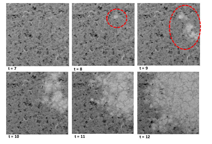
Refer to caption — Figure 2: A sequence of metal corrosion images. The time (index for the image in the sequence) is labeled; the corrosion initiates at time $t=8$ (marked by red circle) and develops over time.

The dynamics of the signal model, in terms of the definition in (5.2), has the following parameters: $\alpha_{t,1}=1$ , and $\alpha_{t,s}=0$ for $s>1$ ; $p(1)=1$ and $p(s)=0$ for $s>1$ ; $\rho$ is about $1.2\times 10^{2}$ and it is estimated from the real-data.

In the example, we set the risk tolerance $\epsilon=0.1$ , and let $\vartheta=0.5$ . To evaluate detection performance, we run 3000 Monte Carlo trials and add zero-mean Gaussian noise (with variance 25) to the images. To estimate the noise variance $\sigma^{2}$ , we use the empirical estimation obtained taking the first 5 noisy images in the sequence (hence we assume they do not contain a rust spot). The corresponding estimation is 25.

Since the rust signal is local, i.e., when it occurs, a cluster of pixels captures the rust, we will apply our detector in the following scheme. Break each image into (rectangular or square) patches of equal size. Design a quadratic detector as described above for a patch. Then at each time, whenever one patch detects a change, we claim there has been a change - this corresponds to a “multi-sensor” scheme and the local detection statistic by taking their maximum.

We compare our quadratic detector to the “sliding window” (Sl-W) detector developed in [18, 12] and defined as follows. Given “window width” $h\in\{1,2,...\}$ and denoting by $y_{tj}$ the vector of observations at time $t$ in patch $j$ , we build the left and the right estimates, ${\bar{y}}_{\ell j}^{t}(h)$ and ${\bar{y}}_{rj}^{t}(h)$ , of $y_{tj}$ :

{\bar{y}}_{\ell j}^{t}(h)=\frac{1}{h}\sum_{i=t-h+1}^{t}y_{ij}\mbox{ and }{\bar{y}}_{rj}^{t}(h)=\frac{1}{h}\sum_{i=t}^{t+h-1}y_{ij}.

At time $t$ , Sl-W always accepts the nuisance hypothesis when $t\leq 2h-2$ ; when $t\geq 2h-1$ , the nuisance hypothesis is accepted if for every patch $j=1,\ldots,N$ , it holds

\max_{h\leq\tau\leq t-h+1}\;\|{\bar{y}}_{\ell j}^{\tau}(h)-{\bar{y}}_{rj}^{\tau}(h)\|_{\infty}\leq\kappa,

and is rejected otherwise. In our experiments, $h=2$ and $h=3$ were used. The corresponding thresholds $\kappa$ are computed using Monte-Carle simulation, see [12] for details.

Simulation results are presented in Table 2. While the performance of Sl-W with properly selected $h$ and the number of patches $N$ is quite good, the quadratic detector is a clear winner in terms of reliability (zero empirical probabilities of a false alarm and a miss), and with $N=49$ , there is no delay in detecting the change.

	Number $K$ of patches
Detector	$K=1$	$K=4$	$K=8$
Sl-W detector, $h=2$	[10.0,11.0,14.0]	[10.0,10.6,14]	[10.0,10.2,14]
Sl-W detector, $h=3$	[10.0,10.9,11.0]	[10.0,10.7,11.0]	[5.0,10.3,11.0]
Quadratic detector	[13.0,13.0,13.0]	[11.0,11.0,11.0]	[10.0,10.0,10.0]
Detector	$K=16$	$K=28$	$K=49$
Sl-W detector, $h=2$	[10.0,10.1,11.0]	[9.0,10.0,11.0]	[10.0,10.1,11]
Sl-W detector, $h=3$	[5.0,9.8,11.0]	[5.0,8.7,10.0]	[5.0,6.8,10.0]
Quadratic detector	[10.0,10.0,10.0]	[10.0,10.0,10.0]	[8.0,8.0,8.0]

Stopping time. Data in a cell

[t_{\min},\bar{t},t_{\max}]

\bar{t}

is the mean, and

[t_{\min},t_{\max}]

is the range of

instant where the signal conclusion has been made. The actual change occurs at time

8

	False alarm probability						Miss detection rate
Nb. of patches	$1$	$4$	$8$	$16$	$28$	$49$	$1$	$4$	$8$	$16$	$28$	$49$
Sl-W detector, $h=2$	0	0	0	0	0	0	0.34	0.01	0	0	0	0
Sl-W detector, $h=3$	0	0	0.006	0.05	0.26	0.64	0	0	0	0	0	0
Quadratic detector	0	0	0	0	0	0	0	0	0	0	0	0

Probabilities of false alarm and miss rates.

Table 2: Numerical results for rust detection

References

[1] M. Basseville and I. Nikiforov. Detection of Abrupt Changes: Theory and Application. Prentice-Hall, Englewood Cliffs, N.J., 1993.
[2] E. Brodsky and B. S. Darkhovsky. Nonparametric methods in change point problems, volume 243. Springer Science & Business Media, 2013.
[3] Y. Cao, S. Zhu, Y. Xie, J. Key, J. Kacher, R. R. Unocic, and C. M. Rouleau. Sequential adaptive detection for in-situ transmission electron microscopy (tem). arXiv preprint arXiv:1710.11297, 2017.
[4] J. Chen and A. Gupta. Parametric statistical change point analysis: with applications to genetics, medicine, and finance. Boston: Birkhäuser, 2012.
[5] F. Enikeeva and Z. Harchaoui. High-dimensional change-point detection with sparse alternatives. arXiv preprint arXiv:1312.1900, 2013.
[6] G. Fellouris and G. Sokolov. Second-order asymptotic optimality in multisensor sequential change detection. IEEE Transactions on Information Theory, 62(6):3662–3675, 2016.
[7] N. H. Gholson and R. L. Moose. Maneuvering target tracking using adaptive state estimation. IEEE Transactions on Aerospace and Electronic Systems, 13(3):310–317, 1977.
[8] A. Goldenshluger, A. Juditsky, and A. Nemirovski. Hypothesis testing by convex optimization. Electronic Journal of Statistics, 9(2):1645–1712, 2015.
[9] A. Goldenshluger, A. Juditsky, A. Tsybakov, and A. Zeevi. Change–point estimation from indirect observations. 1. minimax complexity. Ann. Inst. Henri Poincare Probab. Stat., 44:787–818, 2008.
[10] A. Goldenshluger, A. Juditsky, A. Tsybakov, and A. Zeevi. Change-point estimation from indirect observations. 2. adaptation. Ann. Inst. H. Poincare Probab. Statist, 44(5):819–836, 2008.
[11] L. Gordon and M. Pollak. An efficient sequential nonparametric scheme for detecting a change of distribution. The Annals of Statistics, pages 763–804, 1994.
[12] V. Guigues. Nonparametric multidimensional breakpoint detection for the mean and correlations of a discrete time stochastic process. Journal of Nonparametric Statistics, 24:857–882, 2012.
[13] Y. I. Ingster, C. Pouet, and A. B. Tsybakov. Classification of sparse high-dimensional vectors. Philosophical Transactions of the Royal Society of London A: Mathematical, Physical and Engineering Sciences, 367(1906):4427–4448, 2009.
[14] Y. I. Ingster and I. A. Suslina. On detection of a signal of known shape in multi-channel system. Zapiski Nauchnykh Seminarov POMI, 294:88–112, 2002.
[15] Y. I. Ingster, A. B. Tsybakov, and N. Verzelen. Detection boundary in sparse regression. Electron. J. Statist., 4:1476–1526, 2010.
[16] A. Juditski and A. Nemirovski. On sequential hypotheses testing via convex optimization. Automation and Remote Control, 76:809–825, 2015.
[17] A. Juditsky and A. Nemirovski. Hypothesis testing via affine detectors. Electronic Journal of Statistics, 10:2204–2242, 2016.
[18] A. Korostelev and O. Lepski. On a multi-channel change-point problem. Mathematical Methods of Statistics, 17(3):187–197, 2008.
[19] T. L. Lai. Sequential changepoint detection in quality control and dynamical systems. Journal of the Royal Statistical Society. Series B (Methodological), pages 613–658, 1995.
[20] T. L. Lai. Information bounds and quick detection of parameter changes in stochastic systems. IEEE Transactions on Information Theory, 44(7):2917–2929, 1998.
[21] A. Lakhina, M. Crovella, and C. Diot. Diagnosing network-wide traffic anomalies. In ACM SIGCOMM Computer Communication Review, volume 34, pages 219–230. ACM, 2004.
[22] C. Lévy-Leduc and F. Roueff. Detection and localization of change-points in high-dimensional network traffic data. The Annals of Applied Statistics, pages 637–662, 2009.
[23] K. Liu, R. Zhang, and Y. Mei. Scalable sum-shrinkage schemes for distributed monitoring large-scale data streams. arXiv preprint arXiv:1603.08652, 2016.
[24] G. Lorden. Procedures for reacting to a change in distribution. The Annals of Mathematical Statistics, pages 1897–1908, 1971.
[25] E. Mazor, A. Averbuch, Y. Bar-Shalom, and J. Dayan. Interacting multiple model methods in target tracking: a survey. IEEE Transactions on Aerospace and Electronic Systems, 34(1):103–123, 1998.
[26] Y. Mei. Asymptotic optimality theory for decentralized sequential hypothesis testing in sensor networks. IEEE Transactions on Information Theory, 54(5):2072–2089, 2008.
[27] G. V. Moustakides. Optimal stopping times for detecting changes in distributions. The Annals of Statistics, pages 1379–1387, 1986.
[28] M. H. Neumann. Optimal change-point estimation in inverse problems. Scandinavian Journal of Statistics, 24(4):503–521, 1997.
[29] E. Page. Continuous inspection schemes. Biometrika, 41(1/2):100–115, 1954.
[30] M. Pollak. Optimal detection of a change in distribution. The Annals of Statistics, pages 206–227, 1985.
[31] M. Pollak. Average run lengths of an optimal method of detecting a change in distribution. The Annals of Statistics, pages 749–779, 1987.
[32] H. V. Poor and O. Hadjiliadis. Quickest detection, volume 40. Cambridge University Press Cambridge, 2009.
[33] W. A. Shewhart. Economic control of quality of manufactured product. ASQ Quality Press, 1931.
[34] A. N. Shiryaev. On optimum methods in quickest detection problems. Theory of Probability & Its Applications, 8(1):22–46, 1963.
[35] D. Siegmund. Sequential Analysis: Tests and Confidence Intervals. Springer Science & Business Media, 1985.
[36] D. Siegmund and B. Yakir. The statistics of gene mapping. Springer Science & Business Media, 2007.
[37] A. Tartakovsky, I. Nikiforov, and M. Basseville. Sequential analysis: Hypothesis testing and changepoint detection. CRC Press, 2014.
[38] A. G. Tartakovsky and V. V. Veeravalli. Change-point detection in multichannel and distributed systems. Applied Sequential Methodologies: Real-World Examples with Data Analysis, 173:339–370, 2004.
[39] A. G. Tartakovsky and V. V. Veeravalli. Asymptotically optimal quickest change detection in distributed sensor systems. Sequential Analysis, 27(4):441–475, 2008.
[40] V. V. Veeravalli and T. Banerjee. Quickest change detection. Academic press library in signal processing: Array and statistical signal processing, 3:209–256, 2013.
[41] A. S. Willsky. Detection of abrupt changes in dynamic systems. Springer, 1985.
[42] Y. Xie and D. Siegmund. Sequential multi-sensor change-point detection. Annals of Statistics, 41(2):670–692, 2013.

Appendix A Proofs

A.1 Proof of Lemma 3.1

Recalling what $N^{t}$ and $U^{t}_{k\rho}$ are, we have

{\cal SV}_{tk}(\rho)=\min\limits_{h\in{\mathbf{R}}^{\nu_{t}}}\max\limits_{\begin{array}[]{c}z,v,w,\Theta:\\ z\in N,v\in V_{k},w\in W_{k},\\ v+\rho w\in X,\Theta\in{\cal U}_{t}\\ \end{array}}\left[\mbox{\small$\frac{1}{2}$}h^{T}\bar{A}_{t}[v+\rho w-z]+\mbox{\small$\frac{1}{2}$}h^{T}\Theta h\right].

From compactness of $X$ and $N$ it follows that the domain of the right hand side saddle point problem is nonempty for all $\rho\in\Delta_{k}$ , and from the fact that ${\cal U}_{t}$ is a compact set contained in the interior of the positive semidefinite cone it follows that the saddle point of the right hand side exists for all $\rho\in\Delta_{k}$ . We also clearly have

\begin{array}[]{rcl}{\cal SV}_{tk}(\rho)&=&\max\limits_{\begin{array}[]{c}z,v,w,\Theta:\\ z\in N,v\in V_{k},w\in W_{k},\\ v+\rho w\in X,\Theta\in{\cal U}_{t}\\ \end{array}}\underline{\Psi}_{t}(z,v+\rho w,\Theta),\\ \underline{\Psi}_{t}(p,q,\Theta):&=&-{1\over 8}[p-q]^{T}[\bar{A}_{t}^{T}\Theta^{-1}\bar{A}_{t}][p-q],\\ \end{array}

(A.1)

which combines with compactness of $N$ , $X$ , and ${\cal U}_{t}$ and with the inclusion ${\cal U}_{t}\subset\mathop{\hbox{\rm int}}{\mathbf{S}}^{\nu_{t}}_{+}$ to imply that ${\cal SV}_{tk}(\rho)$ is nonpositive and continuous on $\Delta_{k}$ . From the same representation, due to semi-conicity of $W_{k}$ , it follows that ${\cal SV}_{tk}(\rho)$ is non-increasing in $\rho\in\Delta_{k}$ , and that $\liminf_{\rho\to+0}{\cal SV}_{tk}(\rho)\geq 0$ due to $0\in N$ and $0\in V_{k}$ (this was assumed in Section 3.1), which combines with the fact that ${\cal SV}_{tk}(\rho)$ is nonpositive to imply that $\lim_{\rho\to+0}{\cal SV}_{tk}(\rho)=0$ . It remains to prove that ${\cal SV}_{tk}(\rho)$ is concave. To this end note that when $\rho\in\Delta_{k}$ , the maximum in (A.1) is achieved, and that $\underline{\Psi}_{t}(\cdot)$ is concave by the Schur Complement Lemma. Now let $\rho^{\prime},\rho^{\prime\prime}\in\Delta_{k}$ , $\alpha\in[0,1]$ , and $\beta=1-\alpha$ . We can find $z^{\prime},z^{\prime\prime}\in N$ , $v^{\prime},v^{\prime\prime}\in V_{k}$ , $w^{\prime},w^{\prime\prime}\in W_{k}$ and $\Theta^{\prime},\Theta^{\prime\prime}\in{\cal U}_{t}$ such that

\begin{array}[]{l}\underline{\Psi}_{t}(z^{\prime},v^{\prime}+\rho^{\prime}w^{\prime},\Theta^{\prime})={\cal SV}_{tk}(\rho^{\prime}),\underline{\Psi}_{t}(z^{\prime\prime},v^{\prime\prime}+\rho^{\prime\prime}w^{\prime\prime},\Theta^{\prime\prime})={\cal SV}_{tk}(\rho^{\prime\prime}),\\ v^{\prime}+\rho^{\prime}w^{\prime}\in X,\,v^{\prime\prime}+\rho^{\prime\prime}w^{\prime\prime}\in X.\\ \end{array}

Setting

\begin{array}[]{l}\rho=\alpha\rho^{\prime}+\beta\rho^{\prime\prime},z=\alpha z^{\prime}+\beta z^{\prime\prime},v=\alpha v^{\prime}+\beta v^{\prime\prime},\Theta=\alpha\Theta^{\prime}+\beta\Theta^{\prime\prime},\\ w=\rho^{-1}[\alpha\rho^{\prime}w^{\prime}+\beta\rho^{\prime\prime}w^{\prime\prime}]=\frac{\alpha\rho^{\prime}}{\alpha\rho^{\prime}+\beta\rho^{\prime\prime}}w^{\prime}+\frac{\beta\rho^{\prime\prime}}{\alpha\rho^{\prime}+\beta\rho^{\prime\prime}}w^{\prime\prime},\\ \end{array}

we get by convexity of $N,X,V_{k},W_{k},{\cal U}_{t}$ :

z\in N,v\in V_{k},w\in W_{k},\Theta\in{\cal U}_{t},v+\rho w=\alpha[v^{\prime}+\rho^{\prime}w^{\prime}]+\beta[v^{\prime\prime}+\rho^{\prime\prime}w^{\prime\prime}]\in X

and

[z;v+\rho w;\Theta]=\alpha[z^{\prime};v^{\prime}+\rho^{\prime}w^{\prime};\Theta^{\prime}]+\beta[z^{\prime\prime};v^{\prime\prime}+\rho^{\prime\prime}w^{\prime\prime};\Theta^{\prime\prime}].

The latter equality combines with concavity of $\underline{\Psi}_{t}$ to imply that

\begin{array}[]{l}{\cal SV}_{tk}(\alpha\rho^{\prime}+\beta\rho^{\prime\prime})\geq\underline{\Psi}_{t}(z,v+\rho w,\Theta)\\ \geq\alpha\underline{\Psi}_{t}(z^{\prime},v^{\prime}+\rho^{\prime}w^{\prime},\Theta^{\prime})+\beta\underline{\Psi}_{t}(z^{\prime\prime},v^{\prime\prime}+\rho^{\prime\prime}w^{\prime\prime},\Theta^{\prime\prime})=\alpha{\cal SV}_{tk}(\rho^{\prime})+\beta{\cal SV}_{tk}(\rho^{\prime\prime}).\end{array}

The resulting inequality holds true for all $\rho^{\prime},\rho^{\prime\prime}\in\Delta_{k}$ and all $\alpha=1-\beta\in[0,1]$ , so that ${\cal SV}_{tk}(\cdot)$ is concave.

Now let ${\cal U}$ contain the $\succeq$ -largest element $\overline{\Theta}$ , whence the $\nu_{t}\times\nu_{t}$ matrix $\overline{\Theta}_{t}=S_{t}\overline{\Theta}S_{t}^{T}$ , see (2.3), is the $\succeq$ -largest element in ${\cal U}_{t}$ . Then by (A.1) we have

\begin{array}[]{rcl}\Gamma_{tk}(\rho)&:=&\sqrt{-{\cal SV}_{tk}(\rho)}=\min\limits_{\begin{array}[]{c}z,v,w:\\ z\in N,v\in V_{k},w\in W_{k},\\ v+\rho w\in X\end{array}}\|H_{t}[v+\rho w-z]\|_{2},\\ H_{t}&=&{1\over 2\sqrt{2}}[\bar{A}_{t}^{T}[\overline{\Theta}_{t}]^{-1}\bar{A}_{t}]^{1/2},\\ \end{array}

and from the part of the lemma we have just proved we know that $\Gamma_{tk}(\rho)$ is a continuous nonnegative and nondecreasing function of $\rho\in\Delta_{k}$ such that $\lim_{\rho\to+0}\Gamma_{tk}(\rho)=0$ . Given $\rho^{\prime},\rho^{\prime\prime}\in\Delta_{k}$ and taking into account the compactness of $N$ , $V_{k}$ , and $X$ , we can find $z^{\prime},v^{\prime},w^{\prime},z^{\prime\prime},v^{\prime\prime},w^{\prime\prime}$ such that

\begin{array}[]{c}z^{\prime},z^{\prime\prime}\in N,v^{\prime},v^{\prime\prime}\in V_{k},w^{\prime},w^{\prime\prime}\in W_{k},v^{\prime}+\rho^{\prime}w^{\prime}\in X,v^{\prime\prime}+\rho^{\prime\prime}w^{\prime\prime}\in X,\\ \Gamma_{tk}(\rho^{\prime})=\|H_{t}[v^{\prime}+\rho^{\prime}w^{\prime}-z^{\prime}]\|_{2},\Gamma_{tk}(\rho^{\prime\prime})=\|H_{t}[v^{\prime\prime}+\rho^{\prime\prime}w^{\prime\prime}-z^{\prime\prime}]\|_{2}.\\ \end{array}

Now, given $\alpha\in[0,1]$ and setting $\beta=1-\alpha$ ,

[\rho;z;v]=\alpha[\rho^{\prime};z^{\prime};v^{\prime}]+\beta[\rho^{\prime\prime};z^{\prime\prime};v^{\prime\prime}],\,w=\rho^{-1}[\alpha\rho^{\prime}w^{\prime}+\beta\rho^{\prime\prime}w^{\prime\prime}],

we clearly have $z\in N$ , $v\in V_{k}$ , $w\in W_{k}$ , $v+\rho w=\alpha[v^{\prime}+\rho^{\prime}w^{\prime}]+\beta[v^{\prime\prime}+\rho^{\prime\prime}w^{\prime\prime}]\in X$ and therefore

\begin{array}[]{rcl}\Gamma_{tk}(\rho)&\leq&\|H_{t}[v+\rho w-z]\|_{2}=\|H_{t}[\alpha[v^{\prime}+\rho^{\prime}w^{\prime}-z^{\prime}]+\beta[v^{\prime\prime}+\rho^{\prime\prime}w^{\prime\prime}-z^{\prime\prime}]]\|_{2}\\ &\leq&\alpha\Gamma_{tk}(\rho^{\prime})+\beta\Gamma_{tk}(\rho^{\prime\prime}),\end{array}

and convexity of $\Gamma_{tk}(\cdot)$ follows. $\Box$

A.2 Proof of Proposition 3.2

(i) Let the input be a nuisance, and let $t\in\{1,...,d\}$ . The distribution $P$ of observation $y^{t}$ in this case belongs to ${\cal SG}[N^{t},{\cal U}_{t}]$ . Now let $k$ be such that $\rho_{tk}<\infty$ . Invoking the first inequality in (3.8) with $\rho$ set to $\rho_{tk}$ , we see that

\int_{{\mathbf{R}}^{\nu_{t}}}\exp\{-\phi_{tk}(y^{t})\}P(dy^{t})\leq\epsilon_{tk\rho_{tk}}=\exp\{{\cal SV}_{tk}(\rho_{tk})\}=\varkappa_{t}

(see (3.7) and (3.11)). Consequently, $P$ -probability of the event ${\cal E}_{k}=\{\xi^{t}:\,\phi_{tk}(y^{t})<\alpha_{t}\}$ is at most $\varkappa_{t}\exp\{\alpha_{t}\}={\varkappa_{t}^{2}\over\epsilon}$ . The signal conclusion at step $t$ is made only when one of the events ${\cal E}_{k},\,k\in{\cal K}_{t}(\varkappa_{t})$ , takes place, and $P$ -probability of such outcome is at most $K_{t}(\varkappa_{t}){\varkappa_{t}^{2}\over\epsilon}$ . We remark that the latter quantity is $\leq\epsilon_{t}$ by (3.10).

(ii) Now assume that $t$ and $k$ are such that $\rho_{tk}<\infty$ , and that the input belongs to $X^{\rho}_{k}$ with $\rho\geq\rho_{tk}$ . Since $X^{\rho}_{k}$ shrinks when $\rho$ grows, the input in fact belongs to $X^{\rho_{tk}}_{k}$ , and therefore the distribution $P$ of observation $y^{t}$ belongs to ${\cal SG}[U^{t}_{k\rho_{tk}},{\cal U}_{t}]$ . Invoking the second inequality in (3.8), we get

\int_{{\mathbf{R}}^{\nu_{t}}}\exp\{\phi_{tk}(y^{t})\}P(dy^{t})\leq\epsilon_{tk\rho_{tk}}=\exp\{{\cal SV}_{tk}(\rho_{tk})\}=\varkappa_{t}

(see (3.7) and (3.11)). Hence, $P$ -probability of the event ${\cal E}^{c}_{k}=\{\xi^{t}:\,\phi_{tk}(y^{t})\geq\alpha_{t}\}$ is at most $\exp\{-\alpha_{t}\}\varkappa_{t}=\epsilon.$ $\Box$

A.3 Proof of Proposition 3.3

(i) Let the input be a nuisance, and let $t\in\{1,...,d\}$ . The distribution $P$ of observation $y^{t}$ in this case belongs to ${\cal G}[N^{t},{\cal U}_{t}]$ . Now let $k$ be such that $\rho_{tk}<\infty$ . Invoking $(\#)$ and taking into account that, as it was already explained, $\alpha$ as given by (3.18) satisfies $\alpha\leq\delta_{t}^{2}$ , we conclude that the inequality in (3.17. $a$ ) holds, that is,

\begin{array}[]{l}\hbox{\rm Prob}_{y^{t}\sim P}\left\{\phi_{tk}(y^{t})<\alpha\right\}\leq{\mathop{\hbox{\small\rm Erf}}}(\delta_{t}-\alpha/\delta_{t})\\ \quad={\mathop{\hbox{\small\rm Erf}}}\left(\delta_{t}-\mbox{\small$\frac{1}{2}$}[{\mathop{\hbox{\small\rm ErfInv}}}(\epsilon)-{\mathop{\hbox{\small\rm ErfInv}}}(\epsilon_{t}/L_{t}(\delta_{t}))]\right)\hbox{\ [by (\ref{eqalphabeta})]}\\ \quad\leq{\mathop{\hbox{\small\rm Erf}}}\left(\mbox{\small$\frac{1}{2}$}[{\mathop{\hbox{\small\rm ErfInv}}}(\epsilon)+{\mathop{\hbox{\small\rm ErfInv}}}(\epsilon_{t}/L_{t}(\delta_{t}))]-\mbox{\small$\frac{1}{2}$}[{\mathop{\hbox{\small\rm ErfInv}}}(\epsilon)-{\mathop{\hbox{\small\rm ErfInv}}}(\epsilon_{t}/L_{t}(\delta_{t}))]\right)\\ \qquad\quad\hbox{\ [by (\ref{eq801}) and since ${\mathop{\hbox{\small\rm Erf}}}(\cdot)$ is nonincreasing]}\\ \quad=\min[\epsilon_{t}/L_{t}(\delta_{t}),1/2].\end{array}

This implies that the probability to come to the signal conclusion at step $t$ (this conclusion is made only when $L_{t}(\delta_{t})>0$ and $\phi_{tk}(y^{t})<\alpha$ for some $k\in{\cal L}_{t}(\delta_{t})$ ) is at most $L_{t}(\delta_{t})\cdot(\epsilon_{t}/L_{t}(\delta_{t}))=\epsilon_{t}$ , as claimed.

(ii) Now assume that $t$ and $k$ are such that $\rho_{tk}<\infty$ , and that the input belongs to $X^{\rho}_{k}$ with $\rho\geq\rho_{tk}$ . Since $X^{\rho}_{k}$ shrinks when $\rho$ grows, the input in fact belongs to $X^{\rho_{tk}}_{k}$ , and therefore the distribution $P$ of observation $y^{t}$ belongs to ${\cal G}[U^{t}_{k\rho_{tk}},{\cal U}_{t}]$ . Since, as it was already explained, $\beta$ as given by (3.18) satisfies $\beta\leq\delta_{t}^{2}$ , invoking $(\#)$ , we conclude that for our $P$ the inequality in (3.17. $b$ ) holds, that is,

\begin{array}[]{l}\hbox{\rm Prob}_{y^{t}\sim P}\left\{\phi_{tk}(y^{t})\geq\alpha\right\}=\hbox{\rm Prob}_{y^{t}\sim P}\left\{\phi_{tk}(y^{t})\geq-\beta\right\}\leq{\mathop{\hbox{\small\rm Erf}}}(\delta_{t}-\beta/\delta_{t})\\ \quad={\mathop{\hbox{\small\rm Erf}}}\left(\delta_{t}+\mbox{\small$\frac{1}{2}$}[{\mathop{\hbox{\small\rm ErfInv}}}(\epsilon)-{\mathop{\hbox{\small\rm ErfInv}}}(\epsilon_{t}/L_{t}(\delta_{t}))]\right)\hbox{\ [by (\ref{eqalphabeta})]}\\ \quad\leq{\mathop{\hbox{\small\rm Erf}}}\left(\mbox{\small$\frac{1}{2}$}[{\mathop{\hbox{\small\rm ErfInv}}}(\epsilon)+{\mathop{\hbox{\small\rm ErfInv}}}(\epsilon_{t}/L_{t}(\delta_{t}))]+\mbox{\small$\frac{1}{2}$}[{\mathop{\hbox{\small\rm ErfInv}}}(\epsilon)-{\mathop{\hbox{\small\rm ErfInv}}}(\epsilon_{t}/L_{t}(\delta_{t}))]\right)\\ \qquad\quad\hbox{\ [by (\ref{eq801}) and since ${\mathop{\hbox{\small\rm Erf}}}(\cdot)$ is nonincreasing]}\\ \quad=\epsilon.\end{array}

In other words, in the situation in question, $P$ -probability to terminate at time $t$ with the signal conclusion (which is made when $\phi_{tk^{\prime}}(y^{t})<\alpha$ for some $k^{\prime}$ with $\rho_{tk^{\prime}}<\infty$ ) is at least $1-\epsilon$ . $\Box$

A.4 Proof of Proposition 3.4

Let us refer to the three situations listed in (3.21) as to cases I, II and III. Let $\bar{\rho}=\chi\rho_{tk}^{*}$ , with $\chi$ satisfying (3.21). It may happen that $\bar{\rho}>R_{k}$ ; in this case we have nothing to prove, since there do not exist feasible signals of shape $k$ and magnitude $\geq\bar{\rho}$ . Now let

\bar{\rho}\leq R_{k}.

(A.2)

The function ${\cal SV}_{tk}(\rho)$ is concave on $(0,R_{k}]$ , tends to 0 as $\rho\to+0$ and is equal to $-\mbox{\small$\frac{1}{2}$}{\mathop{\hbox{\small\rm ErfInv}}}^{2}(\epsilon)$ when $\rho=\rho_{tk}^{*}$ . Since $\chi\geq 1$ , we conclude that ${\cal SV}_{tk}(\bar{\rho})\leq\chi{\cal SV}_{tk}(\rho_{tk}^{*})$ , implying in case II that

\begin{array}[]{rcl}{\cal SV}_{tk}(\bar{\rho})&<&-\mbox{\small$\frac{1}{2}$}{\mathop{\hbox{\small\rm ErfInv}}}^{2}(\epsilon)\left(\mbox{\small$\frac{1}{2}$}\left[1+{{\mathop{\hbox{\small\rm ErfInv}}}(\epsilon/(Kd))\over{\mathop{\hbox{\small\rm ErfInv}}}(\epsilon)}\right]\right)^{2}\\ &=&-\mbox{\small$\frac{1}{2}$}\left(\mbox{\small$\frac{1}{2}$}\left[{\mathop{\hbox{\small\rm ErfInv}}}(\epsilon)+{\mathop{\hbox{\small\rm ErfInv}}}(\epsilon/(Kd))\right]\right)^{2},\\ \end{array}

(A.3)

and in case III – that

{\cal SV}_{tk}(\bar{\rho})<\ln(\bar{\varkappa}),\,\,\bar{\varkappa}=\epsilon/\sqrt{Kd}.

(A.4)

In case I, by Lemma 3.1, the function $\sqrt{-{\cal SV}_{tk}(\rho)}$ is convex on $(0,R_{k}]$ , and therefore the same argument as above shows that $\sqrt{-{\cal SV}_{tk}(\bar{\rho})}\geq\chi\sqrt{-{\cal SV}_{tk}(\rho_{tk}^{*})}$ . That is, ${\cal SV}_{tk}(\bar{\rho})\leq\chi^{2}{\cal SV}_{tk}(\rho_{tk}^{*})$ , and we again arrive at (A.3).

Let us now consider the Gaussian case. As we have seen, in this case

{\cal SV}_{tk}(\bar{\rho})<-\mbox{\small$\frac{1}{2}$}\bar{\delta}^{2},\,\,\bar{\delta}=\mbox{\small$\frac{1}{2}$}\left[{\mathop{\hbox{\small\rm ErfInv}}}(\epsilon_{t}/K)+{\mathop{\hbox{\small\rm ErfInv}}}(\epsilon)\right].

(A.5)

Taking into account that $L_{t}(\bar{\delta})\leq K$ and that ${\mathop{\hbox{\small\rm ErfInv}}}(\cdot)$ is non-increasing, we conclude that

\bar{\delta}\geq\mbox{\small$\frac{1}{2}$}\left[{\mathop{\hbox{\small\rm ErfInv}}}(\epsilon)+{\mathop{\hbox{\small\rm ErfInv}}}(\epsilon_{t}/L_{t}(\bar{\delta}))\right],

which combines with (3.13) to imply that $\bar{\delta}\geq\delta_{t}$ . Consequently, by (A.5), we have ${\cal SV}_{tk}(\bar{\rho})<-\mbox{\small$\frac{1}{2}$}\delta_{t}^{2}$ , and since we are in the case where (A.2) holds and ${\cal SV}$ is non-increasing, we have ${\cal SV}_{tk}(R_{k})<-\mbox{\small$\frac{1}{2}$}\delta_{t}^{2}$ as well. Hence, $k\in{\cal L}_{t}(\delta_{t})$ , therefore $\rho_{tk}<\infty$ , and, in addition, $\bar{\rho}>\rho_{tk}$ (since for finite $\rho_{tk}$ we have ${\cal SV}_{tk}(\rho_{tk})=-\mbox{\small$\frac{1}{2}$}\delta_{t}^{2}$ , while ${\cal SV}_{tk}(\bar{\rho})<-\mbox{\small$\frac{1}{2}$}\delta_{t}^{2}$ and ${\cal SV}$ is nonincreasing). Thus, we are in the case of $\rho_{tk}\leq\bar{\rho}\leq R_{k}$ , and therefore, by item (ii) of Proposition 3.3, for a feasible signal of shape $k$ and magnitude $\geq\bar{\rho}$ , the probability for the inference procedure from Section 3.3 to terminate at time $t$ with the signal conclusion is at least $1-\epsilon$ , as required.

Now, assume that we are in the sub-Gaussian case. By (A.2) combined with (A.4), we have

{\cal SV}_{tk}(R_{k})<\ln(\bar{\varkappa}).

(A.6)

We claim that

\bar{\varkappa}\leq\varkappa_{t},

(A.7)

where $\varkappa_{t}$ is given by (3.9). Indeed, we have $K_{t}(\bar{\varkappa})\leq K={\epsilon\epsilon_{t}/\bar{\varkappa}^{2}}$ (recall that $\epsilon_{t}=\epsilon/d$ ), which combines with (3.9) to imply (A.7). Besides this, we have

\ln(\bar{\varkappa})\leq-\mbox{\small$\frac{1}{2}$}{\mathop{\hbox{\small\rm ErfInv}}}^{2}(\epsilon).

Indeed, we have $0<{\mathop{\hbox{\small\rm ErfInv}}}(\epsilon)\leq\sqrt{2\ln(1/\epsilon)}$ , whence

-\mbox{\small$\frac{1}{2}$}{\mathop{\hbox{\small\rm ErfInv}}}^{2}(\epsilon)\geq\ln(\epsilon)\geq\ln(\sqrt{\epsilon^{2}/(dK)})=\ln(\bar{\varkappa}).

Invoking (A.6), we get ${\cal SV}_{tk}(R_{k})<\ln(\varkappa_{t})$ by (A.7), that is, recalling the construction from Section 3.2.3, $\rho_{tk}$ is well defined and satisfies

\rho_{tk}\in(0,R_{k})\;\;\mbox{with}\;\;{\cal SV}_{tk}(\rho_{tk})=\ln(\varkappa_{t}).

(A.8)

Because ${\cal SV}_{tk}(\rho)$ is nonincreasing, we conclude from (A.4), (A.7) and the second relation in (A.8) that $\bar{\rho}\geq\rho_{tk}$ . Invoking item (ii) of Proposition 3.2, we conclude that if the input is a feasible signal with activation of shape $k$ and magnitude at least $\bar{\rho}$ , the probability of the inference routine from Section 3.2.3 to terminate at time $t$ with the signal conclusion is at least $1-\epsilon$ . $\Box$

A.5 Proof of Proposition 4.1

Observe that when $m,\nu\in{\mathbf{R}}^{n}$ and $S\in{\mathbf{S}}^{n}$ , $\|S\|<1$ , one has

\begin{array}[]{l}\ln\Big({\mathbf{E}}_{\xi\sim{\cal N}(\nu,I_{n})}\left\{\exp\{m^{T}\xi+\frac{1}{2}\xi^{T}S\xi\}\right\}\Big)\\ \hskip 9.24994pt=-\frac{1}{2}\ln{\hbox{\rm Det}}(I_{n}-S)+m^{T}\nu+\frac{1}{2}\nu^{T}S\nu+\frac{1}{2}(m+S\nu)^{T}[I_{n}-S]^{-1}(m+S\nu).\\ \end{array}

(A.9)

Indeed,

\begin{array}[]{l}{\mathbf{E}}_{\xi\sim{\cal N}(\nu,I_{n})}\left\{\exp\{m^{T}\xi+\frac{1}{2}\xi^{T}S\xi\}\right\}\\ ={1\over(2\pi)^{n/2}}\exp\{m^{T}\nu+{1\over 2}\nu^{T}S\nu\}\int\exp\{d^{T}\eta-{1\over 2}\eta^{T}[I_{n}-S]\eta\}d\eta\\ \lx@intercol\hfil\hbox{\ [$d=m+S\nu$,\,$\eta=\xi-\nu$]}\lx@intercol\\ ={1\over(2\pi)^{n/2}}\exp\{m^{T}\nu+{1\over 2}\nu^{T}S\nu\}\int\exp\{-{1\over 2}\zeta^{T}[I_{n}-S]\zeta+{1\over 2}d^{T}[I_{n}-S]^{-1}d\}d\zeta\\ \lx@intercol\hfil\hbox{\ [$\zeta=\eta-[I_{n}-S]^{-1}d$]}\lx@intercol\\ =\exp\{m^{T}\nu+{1\over 2}\nu^{T}S\nu+{1\over 2}d^{T}[I_{n}-S]^{-1}d\}{\hbox{\rm Det}}^{-1/2}(I_{n}-S)\left[{1\over(2\pi)^{n/2}}\int\exp\{-{1\over 2}\omega^{T}\omega\}d\omega\right]\\ \lx@intercol\hfil\hbox{\ [$\omega=[I_{n}-S]^{1/2}\zeta$]}\lx@intercol\\ =\exp\{m^{T}\nu+{1\over 2}\nu^{T}S\nu+{1\over 2}d^{T}[I_{n}-S]^{-1}d\}{\hbox{\rm Det}}^{-1/2}(I_{n}-S),\\ \end{array}

which is exactly (A.9).

A.5.1 Proof of Proposition 4.1.i

1⁰.

Let $b=[0;...;0;1]\in{\mathbf{R}}^{n+1}$ , so that $B=\left[\begin{array}[]{c}A\cr b^{T}\cr\end{array}\right]$ , and let ${\cal A}(u)=A[u;1]$ . For any $u\in{\mathbf{R}}^{n}$ , $h\in{\mathbf{R}}^{\nu},\;\Theta\in{\mathbf{S}}^{\nu}_{+}$ and $H\in{\mathbf{S}}^{\nu}$ such that $-I\prec\Theta^{1/2}H\Theta^{1/2}\prec I$ , we have

\begin{array}[]{l}\Psi(h,H;u,\Theta):=\ln\left({\mathbf{E}}_{\zeta\sim{\cal N}({\cal A}(u),\Theta)}\left\{\exp\{h^{T}\zeta+\mbox{\small$\frac{1}{2}$}\zeta^{T}H\zeta\}\right\}\right)\\ =\hbox{\small$\ln\left({\mathbf{E}}_{\xi\sim{\cal N}(0,I)}\left\{\exp\{h^{T}[{\cal A}(u)+\Theta^{1/2}\xi]+\mbox{\small$\frac{1}{2}$}[{\cal A}(u)+\Theta^{1/2}\xi]^{T}H[{\cal A}(u)+\Theta^{1/2}\xi]\}\right\}\right)$}\\ =-\mbox{\small$\frac{1}{2}$}\ln{\hbox{\rm Det}}(I-\Theta^{1/2}H\Theta^{1/2})+h^{T}{\cal A}(u)\\ \quad+\mbox{\small$\frac{1}{2}$}{\cal A}(u)^{T}H{\cal A}(u)+\mbox{\small$\frac{1}{2}$}[H{\cal A}(u)+h]^{T}\Theta^{1/2}[I-\Theta^{1/2}H\Theta^{1/2}]^{-1}\Theta^{1/2}[H{\cal A}(u)+h]\\ \lx@intercol\hfil\hbox{[by (\ref{newformula})]}\lx@intercol\\ =-\mbox{\small$\frac{1}{2}$}\ln{\hbox{\rm Det}}(I-\Theta^{1/2}H\Theta^{1/2})+\mbox{\small$\frac{1}{2}$}[u;1]^{T}\left[bh^{T}A+A^{T}hb^{T}+A^{T}HA\right][u;1]\\ \quad+\mbox{\small$\frac{1}{2}$}[u;1]^{T}\left[B^{T}[H,h]^{T}\Theta^{1/2}[I-\Theta^{1/2}H\Theta^{1/2}]^{-1}\Theta^{1/2}[H,h]B\right][u;1]\\ \end{array}

(A.10)

(because $h^{T}{\cal A}(u)=[u;1]^{T}bh^{T}A[u;1]=[u;1]^{T}A^{T}hb^{T}[u;1]$ and $H{\cal A}(u)+h=[H,h]B[u;1]$ ).

Observe that when $(h,H)\in{\cal H}^{\gamma}$ , we have $\Theta^{1/2}[I-\Theta^{1/2}H\Theta^{1/2}]^{-1}\Theta^{1/2}=[\Theta^{-1}-H]^{-1}\preceq[\Theta_{*}^{-1}-H]^{-1},$ so that (A.10) implies that for all $u\in{\mathbf{R}}^{n},\;\Theta\in{\cal U},$ and $(h,H)\in{\cal H}^{\gamma}$ ,

\begin{array}[]{rcl}\Psi(h,H;u,\Theta)&\leq&-\mbox{\small$\frac{1}{2}$}\ln{\hbox{\rm Det}}(I-\Theta^{1/2}H\Theta^{1/2})\\ \lx@intercol\hfil+\mbox{\small$\frac{1}{2}$}[u;1]^{T}\underbrace{\left[bh^{T}A+A^{T}hb^{T}+A^{T}HA+B^{T}[H,h]^{T}[\Theta_{*}^{-1}-H]^{-1}[H,h]B\right]}_{Q[H,h]}[u;1]\lx@intercol\\ &=&-\mbox{\small$\frac{1}{2}$}\ln{\hbox{\rm Det}}(I-\Theta^{1/2}H\Theta^{1/2})+\mbox{\small$\frac{1}{2}$}{\hbox{\rm Tr}}(Q[H,h]Z(u))\\ &\leq&-\mbox{\small$\frac{1}{2}$}\ln{\hbox{\rm Det}}(I-\Theta^{1/2}H\Theta^{1/2})+\Gamma_{{\cal Z}}(h,H),\\ \Gamma_{{\cal Z}}(h,H)&=&\mbox{\small$\frac{1}{2}$}\phi_{{\cal Z}}(Q[H,h])\\ \end{array}

(A.11)

(we have taken into account that $Z(u)\in{\cal Z}$ when $u\in U$ (premise of the proposition) and therefore ${\hbox{\rm Tr}}(Q[H,h]Z(u))\leq\phi_{{\cal Z}}(Q[H,h])$ ).

2⁰.

We need the following:

Lemma A.1.

Let $\Theta_{*}$ be a $d\times d$ symmetric positive definite matrix, let $\delta\in[0,2]$ , and let ${\cal U}$ be a closed convex subset of ${\mathbf{S}}^{d}_{+}$ such that

\Theta\in{\cal U}\Rightarrow\{\Theta\preceq\Theta_{*}\}\ \&\ \{\|\Theta^{1/2}\Theta_{*}^{-1/2}-I\|\leq\delta\}

(A.12)

(cf. (4.1)). Let also ${\cal H}^{o}:=\{H\in{\mathbf{S}}^{d}:-\Theta_{*}^{-1}\prec H\prec\Theta_{*}^{-1}\}$ . Then

\begin{array}[]{l}\forall(H,\Theta)\in{\cal H}^{o}\times{\cal U}:\\ G(H;\Theta):=-\mbox{\small$\frac{1}{2}$}\ln{\hbox{\rm Det}}(I-\Theta^{1/2}H\Theta^{1/2})\\ \quad\leq G^{+}(H;\Theta):=-\mbox{\small$\frac{1}{2}$}\ln{\hbox{\rm Det}}(I-\Theta_{*}^{1/2}H\Theta_{*}^{1/2})+\mbox{\small$\frac{1}{2}$}{\hbox{\rm Tr}}([\Theta-\Theta_{*}]H)\\ \lx@intercol\hfil+{\delta(2+\delta)\over 2(1-\|\Theta_{*}^{1/2}H\Theta_{*}^{1/2}\|)}\|\Theta_{*}^{1/2}H\Theta_{*}^{1/2}\|_{F}^{2},\lx@intercol\\ \end{array}

(A.13)

where $\|\cdot\|$ is the spectral, and $\|\cdot\|_{F}$ - the Frobenius norm of a matrix. In addition, $G^{+}(H,\Theta)$ is a continuous function on ${\cal H}^{o}\times{\cal U}$ which is convex in $H\in{{\cal H}^{o}}$ and concave (in fact, affine) in $\Theta\in{\cal U}$ .

Proof. Let us set

d(H)=\|\Theta_{*}^{1/2}H\Theta_{*}^{1/2}\|,

so that $d(H)<1$ for $H\in{\cal H}^{o}$ . For $H\in{\cal H}^{o}$ and $\Theta\in{\cal U}$ fixed we have

\begin{array}[]{rcl}\|\Theta^{1/2}H\Theta^{1/2}\|&=&\|[\Theta^{1/2}\Theta_{*}^{-1/2}][\Theta_{*}^{1/2}H\Theta_{*}^{1/2}][\Theta^{1/2}\Theta_{*}^{-1/2}]^{T}\|\\ &\leq&\|\Theta^{1/2}\Theta_{*}^{-1/2}\|^{2}\|\Theta_{*}^{1/2}H\Theta_{*}^{1/2}\|\leq\|\Theta_{*}^{1/2}H\Theta_{*}^{1/2}\|=d(H)\\ \end{array}

(A.14)

(we have used the fact that $0\preceq\Theta\preceq\Theta_{*}$ implies $\|\Theta^{1/2}\Theta_{*}^{-1/2}\|\leq 1$ ). Noting that $\|AB\|_{F}\leq\|A\|\|B\|_{F}$ , a computation completely similar to the one in (A.14) yields

\|\Theta^{1/2}H\Theta^{1/2}\|_{F}\leq\|\Theta_{*}^{1/2}H\Theta_{*}^{1/2}\|_{F}=:D(H).

(A.15)

Besides this, setting $F(X)=-\ln{\hbox{\rm Det}}(X):\mathop{\hbox{\rm int}}{\mathbf{S}}^{d}_{+}\to{\mathbf{R}}$ and equipping ${\mathbf{S}}^{d}$ with the Frobenius inner product, we have $\nabla F(X)=-X^{-1}$ , so that with $R_{0}=\Theta_{*}^{1/2}H\Theta_{*}^{1/2}$ , $R_{1}=\Theta^{1/2}H\Theta^{1/2}$ , and $\Delta=R_{1}-R_{0}$ , we have for properly selected $\lambda\in(0,1)$ and $R_{\lambda}=\lambda R_{0}+(1-\lambda)R_{1}$ :

$\displaystyle F(I-R_{1})$	$\displaystyle=$	$\displaystyle F(I-R_{0}-\Delta)=F(I-R_{0})+\langle\nabla F(I-R_{\lambda}),-\Delta\rangle$
	$\displaystyle=$	$\displaystyle F(I-R_{0})+\langle(I-R_{\lambda})^{-1},\Delta\rangle$
	$\displaystyle=$	$\displaystyle F(I-R_{0})+\langle I,\Delta\rangle+\langle(I-R_{\lambda})^{-1}-I,\Delta\rangle.$

We conclude that

F(I-R_{1})\leq F(I-R_{0})+{\hbox{\rm Tr}}(\Delta)+\|I-(I-R_{\lambda})^{-1}\|_{F}\|\Delta\|_{F}.

(A.16)

Denoting by $\mu_{i}$ the eigenvalues of $R_{\lambda}$ and noting that $\|R_{\lambda}\|\leq\max[\|R_{0}\|,\|R_{1}\|]=d(H)$ (see (A.14)), we have $|\mu_{i}|\leq d(H)$ , and therefore eigenvalues $\nu_{i}=1-{1\over 1-\mu_{i}}=-{\mu_{i}\over 1-\mu_{i}}$ of $I-(I-R_{\lambda})^{-1}$ satisfy $|\nu_{i}|\leq|\mu_{i}|/(1-\mu_{i})\leq|\mu_{i}|/(1-d(H))$ , whence

\|I-(I-R_{\lambda})^{-1}\|_{F}=\sqrt{{\sum}_{i=1}^{d}\nu_{i}^{2}}\leq\frac{\sqrt{\sum_{i=1}^{d}\mu_{i}^{2}}}{1-d(H)}=\frac{\|R_{\lambda}\|_{F}}{1-d(H)}.

Noting that $\|R_{\lambda}\|_{F}\leq\max[\|R_{0}\|_{F},\|R_{1}\|_{F}]{=}D(H)$ , see (A.15), we conclude that $\|I-(I-R_{\lambda})^{-1}\|_{F}\leq D(H)/(1-d(H))$ , so that (A.16) yields

F(I-R_{1})\leq F(I-R_{0})+{\hbox{\rm Tr}}(\Delta)+D(H)\|\Delta\|_{F}/(1-d(H)).

(A.17)

Further, by (4.1) the matrix $D=\Theta^{1/2}\Theta_{*}^{-1/2}-I$ satisfies $\|D\|\leq\delta$ , whence

\Delta=\underbrace{\Theta^{1/2}H\Theta^{1/2}}_{R_{1}}-\underbrace{\Theta_{*}^{1/2}H\Theta_{*}^{1/2}}_{R_{0}}=(I+D)R_{0}(I+D^{T})-R_{0}=DR_{0}+R_{0}D^{T}+DR_{0}D^{T}.

Consequently,

\begin{array}[]{l}\|\Delta\|_{F}\leq\|DR_{0}\|_{F}+\|R_{0}D^{T}\|_{F}+\|DR_{0}D^{T}\|_{F}\leq[2\|D\|+\|D\|^{2}]\|R_{0}\|_{F}\\ \lx@intercol\hfil\leq\delta(2+\delta)\|R_{0}\|_{F}=\delta(2+\delta)D(H).\lx@intercol\end{array}

This combines with (A.17) and the relation

{\hbox{\rm Tr}}(\Delta)={\hbox{\rm Tr}}(\Theta^{1/2}H\Theta^{1/2}-\Theta_{*}^{1/2}H\Theta_{*}^{1/2})={\hbox{\rm Tr}}([\Theta-\Theta_{*}]H)

to yield

F(I-R_{1})\leq F(I-R_{0})+{\hbox{\rm Tr}}([\Theta-\Theta_{*}]H)+{\delta(2+\delta)\over 1-d(H)}\|\Theta_{*}^{1/2}H\Theta_{*}^{1/2}\|_{F}^{2},

and we arrive at (A.13). It remains to prove that $G^{+}(H;\Theta)$ is convex-concave and continuous on ${\cal H}^{o}\times{\cal U}$ . The only component of this claim which is not completely evident is convexity of the function in $H\in{\cal H}^{o}$ . To see that it is the case, note that $\ln{\hbox{\rm Det}}(S)$ is concave on the interior of the semidefinite cone, the function $f(u,v)={u^{2}\over 1-v}$ is convex and nondecreasing in $u,v$ in the convex domain $\Pi=\{(u,v):u\geq 0,v<1\}$ , and the function ${\|\Theta_{*}^{1/2}H\Theta_{*}^{1/2}\|_{F}^{2}\over 1-\|\Theta_{*}^{1/2}H\Theta_{*}^{1/2}\|}$ is obtained from $f$ by convex substitution of variables $H\mapsto(\|\Theta_{*}^{1/2}H\Theta_{*}^{1/2}\|_{F},\|\Theta_{*}^{1/2}H\Theta_{*}^{1/2}\|)$ mapping ${\cal H}^{o}$ into $\Pi$ . $\Box$ .

3⁰.

Combining (A.13), (A.11), (4.5) and the origin of $\Psi$ , see (A.10), we arrive at

\begin{array}[]{l}\forall((u,\Theta)\in U\times{\cal U},(h,H)\in{\cal H}^{\gamma}={\cal H}):\\ \lx@intercol\hfil\ln\left({\mathbf{E}}_{\zeta\sim{\cal N}({A[u;1]},\Theta)}\left\{\exp\{h^{T}\zeta+\mbox{\small$\frac{1}{2}$}\zeta^{T}H\zeta\}\right\}\right)\leq\Phi_{A,{\cal Z}}(h,H;\Theta),\hfil\lx@intercol\\ \end{array}

as claimed in (4.6).

4⁰.

Now let us check that $\Phi_{A,{\cal Z}}(h,H;\Theta):{\cal H}\times{\cal U}\to{\mathbf{R}}$ is continuous and convex-concave. Recalling that the function $G^{+}(H;\Theta)$ from (A.13) is convex-concave and continuous on ${\cal H}^{o}\times{\cal U}$ , all we need to verify is that $\Gamma_{{\cal Z}}(h,H)$ is convex and continuous on ${\cal H}$ . Recalling that ${\cal Z}$ is a nonempty compact set, the function $\phi_{{\cal Z}}(\cdot):\,{\mathbf{S}}^{n+1}\to{\mathbf{R}}$ is continuous, implying the continuity of $\Gamma_{{\cal Z}}(h,H)=\mbox{\small$\frac{1}{2}$}\phi_{{\cal Z}}(Q[H,h])$ on ${\cal H}={\cal H}^{\gamma}$ ( $Q[H,h]$ is defined in (A.11)). To prove the convexity of $\Gamma$ , note that ${\cal Z}$ is contained in ${\mathbf{S}}^{n+1}_{+}$ , implying that $\phi_{{\cal Z}}(\cdot)$ is convex and $\succeq$ -monotone. On the other hand, by Schur Complement Lemma, we have

\begin{array}[]{rcl}S&:=&\{(h,H,G):G\succeq Q[H,h],(h,H)\in{\cal H}^{\gamma}\}\\ &=&\bigg\{(h,H,G):\left[\begin{array}[]{c|c}G-[bh^{T}A+{A^{T}hb^{T}}+A^{T}HA]&B^{T}[H,h]^{T}\cr\hline\cr[H,h]B&\Theta_{*}^{-1}-H\cr\end{array}\right]\\ &&\lx@intercol\hfil\succeq 0,(h,H)\in{\cal H}^{\gamma}\bigg\},\lx@intercol\\ \end{array}

implying that $S$ is convex. Since $\phi_{{\cal Z}}(\cdot)$ is $\succeq$ -monotone, we have

\begin{array}[]{l}\{(h,H,\tau):(h,H)\in{\cal H}^{\gamma},\;\tau\geq{\Gamma_{\cal Z}}(h,H)\}=\{(h,H,\tau):\exists G:G\succeq Q[H,h],\\ \lx@intercol\hfil 2\tau\geq\phi_{{\cal Z}}(G),\;(h,H)\in{\cal H}^{\gamma}\},\lx@intercol\end{array}

and we see that the epigraph of $\Gamma_{\cal Z}$ is convex (since the set $S$ and the epigraph of $\phi_{{\cal Z}}$ are so), as claimed.

5⁰.

It remains to prove that $\Phi_{{\cal A},{\cal Z}}$ is coercive in $H,h$ . Let $\Theta\in{\cal U}$ and $(h_{i},H_{i})\in{\cal H}^{\gamma}$ with $\|(h_{i},H_{i})\|\to\infty$ as $i\to\infty$ , and let us prove that $\Phi_{{\cal A},{\cal Z}}(h_{i},H_{i};\Theta)\to\infty$ . Looking at the expression for $\Phi_{{\cal A},{\cal Z}}(h_{i},H_{i};\Theta)$ , it is immediately seen that all terms in this expression, except for the terms coming from $\phi_{{\cal Z}}(\cdot)$ , remain bounded as $i$ grows, so that all we need to verify is that the $\phi_{{\cal Z}}(\cdot)$ -term goes to $\infty$ as $i\to\infty$ . Observe that $H_{i}$ are uniformly bounded due to $(h_{i},H_{i})\in{\cal H}^{\gamma}$ , implying that $\|h_{i}\|_{2}\to\infty$ as $i\to\infty$ .
Denoting $e=[0;...;0;1]\in{\mathbf{R}}^{\nu+1}$ and, as before, $b=[0;...;0;1]\in{\color[rgb]{0,0,1}\ {\mathbf{R}}^{n+1}}$ , note that, by construction, $B^{T}e=b$ . Now let $W\in{\cal Z}$ , so that $W_{n+1,n+1}=1$ . Taking into account that the matrices $[\Theta_{*}^{-1}-H_{i}]^{-1}$ satisfy $\alpha I_{d}\preceq[\Theta_{*}^{-1}-H_{i}]^{-1}\preceq\beta I_{d}$ for some positive $\alpha,\beta$ due to $H_{i}\in{\cal H}^{\gamma}$ , we come to

\begin{array}[]{l}\underbrace{\left[\left[\begin{array}[]{c|c}H_{i}&h_{i}\cr\hline\cr h_{i}^{T}&\end{array}\right]+\left[H_{i},h_{i}\right]^{T}[\Theta_{*}^{-1}-H_{i}]^{-1}\left[H_{i},h_{i}\right]\right]}_{Q_{i}}=\underbrace{\left[h_{i}^{T}[\Theta_{*}^{-1}-H_{i}]^{-1}h_{i}\right]}_{\alpha_{i}\|h_{i}\|_{2}^{2}}ee^{T}+R_{i},\\ \end{array}

where $\alpha_{i}\geq\alpha>0$ and $\|R_{i}\|_{F}\leq C(1+\|h_{i}\|_{2})$ . As a result,

\begin{array}[]{rcl}\phi_{{\cal Z}}(B^{T}Q_{i}B)&\geq&{\hbox{\rm Tr}}(WB^{T}Q_{i}B)={\hbox{\rm Tr}}(WB^{T}[\alpha_{i}\|h_{i}\|_{2}^{2}ee^{T}+R_{i}]B)\\ &{\geq}&\alpha_{i}\|h_{i}\|_{2}^{2}\underbrace{{\hbox{\rm Tr}}(Wbb^{T})}_{=W_{n+1,n+1}=1}-\|BWB^{T}\|_{F}\|R_{i}\|_{F}\\ &\geq&\alpha\|h_{i}\|_{2}^{2}-C(1+\|h_{i}\|_{2})\|BWB^{T}\|_{F},\\ \end{array}

and the concluding quantity tends to $\infty$ as $i\to\infty$ due to $\|h_{i}\|_{2}\to\infty$ , $i\to\infty$ . Part (i) is proved.

A.5.2 Proof of Proposition 4.1.ii

Part (ii) of the proposition is a straightforward combination of part (i) and [17, Proposition 3.1]; for the sake of completeness, here is a simple proof. Since by (i) the function $\Phi(h,H;\Theta_{1},\Theta_{2})$ is continuous and convex-concave on the domain $\underbrace{({\cal H}_{1}\cap{\cal H}_{2})}_{{\cal H}}\times\underbrace{({\cal U}_{1}\times{\cal U}_{2})}_{{\cal U}}$ and are coercive in $(h,H)$ , while ${\cal H}$ and ${\cal U}$ are closed and convex, and ${\cal U}$ in addition is compact, saddle point problem (4.7) is solvable (Sion-Kakutani Theorem). Now let $(h_{*},H_{*};\Theta_{1}^{*},\Theta_{2}^{*})$ be a saddle point. To prove (4.9), let $P\in{\cal G}_{1}$ , that is, $P={\cal N}(A_{1}[u;1],\Theta_{1})$ for some $\Theta_{1}\in{\cal U}_{1}$ and some $u$ with $[u;1][u;1]^{T}\in{\cal Z}_{1}$ . Applying (4.6) to the first collection of data, with $a$ given by (4.8), we get the first $\leq$ in the following chain:

\begin{array}[]{l}\ln\left(\displaystyle\int{\rm e}^{-\mbox{\small$\frac{1}{2}$}\omega^{T}H_{*}\omega-\omega^{T}h_{*}-a}P(d\omega)\right)\\ \leq\Phi_{A_{1},{\cal Z}_{1}}(-h_{*},-H_{*};\Theta_{1})-a\underbrace{\leq}_{(a)}\Phi_{A_{1},{\cal Z}_{1}}(-h_{*},-H_{*};\Theta_{1}^{*})-a\underbrace{=}_{(b)}{\cal SV},\\ \end{array}

where $(a)$ is due to the fact that $\Phi_{A_{1},{\cal Z}_{1}}(-h_{*},-H_{*};\Theta_{1})+\Phi_{A_{2},{\cal Z}_{2}}(h_{*},H_{*};\Theta_{2})$ attains its maximum over $(\Theta_{1},\Theta_{2})\in{\cal U}_{1}\times{\cal U}_{2}$ at the point $(\Theta_{1}^{*},\Theta_{2}^{*})$ , and $(b)$ is due to the origin of $a$ and the relation ${\cal SV}=\mbox{\small$\frac{1}{2}$}[\Phi_{A_{1},{\cal Z}_{1}}(-h_{*},-H_{*};\Theta_{1}^{*})+\Phi_{A_{2},{\cal Z}_{2}}(h_{*},H_{*};\Theta_{2}^{*})]$ . The bound in (4.9.a) is proved. Similarly, let $P\in{\cal G}_{2}$ , that is, $P={\cal N}(A_{2}[u;1],\Theta_{2})$ for some $\Theta_{2}\in{\cal U}_{2}$ and some $u$ with $[u;1][u;1]^{T}\in{\cal Z}_{2}$ . Applying (4.6) to the second collection of data, with the same $a$ as above, we get the first $\leq$ in the following chain:

\begin{array}[]{l}\ln\left(\displaystyle\int{\rm e}^{\mbox{\small$\frac{1}{2}$}\omega^{T}H_{*}\omega+\omega^{T}h_{*}+a}P(d\omega)\right)\leq\Phi_{A_{2},{\cal Z}_{2}}(h_{*},H_{*};\Theta_{2})+a\\ \underbrace{\leq}_{(a)}\Phi_{A_{2},{\cal Z}_{2}}(h_{*},H_{*};\Theta_{2}^{*})+a\underbrace{=}_{(b)}{\cal SV},\\ \end{array}

with exactly the same justification as above of $(a)$ and $(b)$ . The bound in (4.9.b) is proved. $\Box$

A.6 Justification for Remark 4.1.

In the easy case, we have $B_{\chi}=I_{\nu+1}$ and therefore

\begin{array}[]{rcl}M_{\chi}(h,H)&:=&B_{\chi}^{T}\left[\hbox{\small$\left[\begin{array}[]{c|c}H&h\cr\hline\cr h^{T}&\end{array}\right]+\left[H,h\right]^{T}\left[[\Theta_{*}^{(\chi)}]^{-1}-H\right]^{-1}\left[H,h\right]$}\right]B_{\chi}\\ &=&\hbox{\small$\left[\begin{array}[]{c|c}H+H\left[[\Theta_{*}^{(\chi)}]^{-1}-H\right]^{-1}H&h+{H}[{[\Theta_{*}^{(\chi)}]^{-1}}-H]^{-1}h\cr\hline\cr h^{T}+h^{T}\left[[\Theta_{*}^{(\chi)}]^{-1}-H\right]^{-1}{H}&h^{T}\left[[\Theta_{*}^{(\chi)}]^{-1}-H\right]^{-1}h\cr\end{array}\right]$}\\ \end{array}

and

\begin{array}[]{rcl}\phi_{{\cal Z}_{\chi}}(Z)&=&\max\limits_{W}\left\{{\hbox{\rm Tr}}(ZW):\,W\succeq 0,\,{\hbox{\rm Tr}}(WQ^{\chi}_{j})\leq q^{\chi}_{j},\,1\leq j\leq J_{\chi}\right\}\\ &=&\min_{\lambda}\left\{\sum_{j}q_{j}^{\chi}\lambda_{j}:\,\lambda\geq 0,\,Z\preceq\sum_{j}\lambda_{j}Q^{\chi}_{j}\right\},\\ \end{array}

where the last equality is due to semidefinite duality. From the second representation of $\phi_{{\cal Z}_{\chi}}(\cdot)$ and the fact that all $Q^{\chi}_{j}$ are diagonal it follows that $\phi_{{\cal Z}_{\chi}}({M_{\chi}}({0,H}))\leq\phi_{{\cal Z}_{\chi}}({M_{\chi}}(h,H))$ (indeed, with diagonal $Q^{\chi}_{j}$ , this representation clearly says that if $\lambda$ is feasible for the minimization problem participating in the representation when $Z=M_{\chi}(h,H)$ , it remains feasible when $Z$ is replaced with $M_{\chi}(0,H)$ ). This, in turn, combines straightforwardly with (4.5) to imply that when replacing $h_{*}$ with $0$ in a saddle point $(h_{*},H_{*};\Theta_{1}^{*},\Theta_{2}^{*})$ of (4.7), we end up with another saddle point of (4.7). In other words, when solving (4.7), we can from the very beginning set $h$ to $0$ , thus converting (4.7) into the convex-concave saddle point problem

{\cal SV}=\min\limits_{H:(0,H)\in{\cal H}_{1}\cap{\cal H}_{2}}\max\limits_{\Theta_{1}\in{\cal U}_{1},\Theta_{2}\in{\cal U}_{2}}\Phi(0,H;\Theta_{1},\Theta_{2}).

(A.18)

Taking into account the fact that we are in the case where all matrices from the sets ${\cal U}_{\chi}$ , same as the matrices $\Theta_{*}^{(\chi)}$ and all the matrices $Q^{\chi}_{j}$ , $\chi=1,2$ , are diagonal, it is immediate to verify that if $E$ is a $\nu\times\nu$ diagonal matrix with diagonal entries $\pm 1$ , then $\Phi(0,H;\Theta_{1},\Theta_{2})=\Phi(0,EHE;\Theta_{1},\Theta_{2})$ . Due to convexity-concavity of $\Phi$ this implies that (A.18) admits a saddle point $(0,H_{*};\Theta_{1}^{*},\Theta_{2}^{*})$ with $H_{*}$ invariant w.r.t. transformations $H_{*}\mapsto EH_{*}E$ with the above $E$ , that is, with diagonal $H_{*}$ , as claimed. $\Box$

A.7 Proof of Proposition 4.2

A.7.1 Preliminaries

We start with the following result:

Lemma A.2.

Let $\bar{\Theta}$ be a positive definite $d\times d$ matrix, and let

u\mapsto{\cal A}(u)=A[u;1]

be an affine mapping from ${\mathbf{R}}^{n}$ into ${\mathbf{R}}^{d}$ . Finally, let $h\in{\mathbf{R}}^{d}$ , $H\in{\mathbf{S}}^{d}$ and $P\in{\mathbf{S}}^{d}$ satisfy the relations

0\preceq P\prec I\ \&\ P\succeq\bar{\Theta}^{1/2}H\bar{\Theta}^{1/2}.

(A.19)

Then, setting $B=\left[\begin{array}[]{cc}A\cr 0,...,0,1\cr\end{array}\right]$ , for every $u\in{\mathbf{R}}^{n}$ it holds

\begin{array}[]{c}\lx@intercol\zeta\sim{\cal SG}({\cal A}(u),{\bar{\Theta}})\Rightarrow\ln\left({\mathbf{E}}_{\zeta}\left\{{\rm e}^{h^{T}\zeta+\mbox{\small$\frac{1}{2}$}\zeta^{T}H\zeta}\right\}\right)\leq-\mbox{\small$\frac{1}{2}$}\ln{\hbox{\rm Det}}(I-P)\hfil\lx@intercol\\ \lx@intercol\hfil+\mbox{\small$\frac{1}{2}$}[u;1]^{T}B^{T}\left[\hbox{\scriptsize$\left[\begin{array}[]{c|c}H&h\cr\hline\cr h^{T}\cr\end{array}\right]$}+\left[H,h\right]^{T}\bar{\Theta}^{1/2}[I-P]^{-1}\bar{\Theta}^{1/2}\left[H,h\right]\right]B[u;1]\lx@intercol.\\ \end{array}

(A.20)

Equivalently (set $G=\bar{\Theta}^{-1/2}P\bar{\Theta}^{-1/2}$ ), whenever $h\in{\mathbf{R}}^{d}$ , $H\in{\mathbf{S}}^{d}$ , and $G\in{\mathbf{S}}^{d}$ satisfy the relations

0\preceq G\prec\bar{\Theta}^{-1}\ \&\ G\succeq H,

(A.21)

one has for every for every $u\in{\mathbf{R}}^{n}$ :

\begin{array}[]{c}\lx@intercol\zeta\sim{\cal SG}({\cal A}(u),\bar{\Theta})\Rightarrow\ln\left({\mathbf{E}}_{\zeta}\left\{{\rm e}^{h^{T}\zeta+\mbox{\small$\frac{1}{2}$}\zeta^{T}H\zeta}\right\}\right)\leq-\mbox{\small$\frac{1}{2}$}\ln{\hbox{\rm Det}}(I-\bar{\Theta}^{1/2}G\bar{\Theta}^{1/2})\hfil\lx@intercol\\ \lx@intercol\hfil+\mbox{\small$\frac{1}{2}$}[u;1]^{T}B^{T}\left[\hbox{\scriptsize$\left[\begin{array}[]{c|c}H&h\cr\hline\cr h^{T}\cr\end{array}\right]$}+\left[H,h\right]^{T}[\bar{\Theta}^{-1}-G]^{-1}\left[H,h\right]\right]B[u;1]\lx@intercol.\end{array}

(A.22)

Proof. 1⁰. Let us start with the following observation:

Lemma A.3.

Let ${\bar{\Theta}}\in{\mathbf{S}}^{d}_{+}$ and $S\in{\mathbf{R}}^{d\times d}$ be such that $S{\bar{\Theta}}S^{T}\prec I_{d}$ . Then for every $\nu\in{\mathbf{R}}^{d}$ one has

\begin{array}[]{l}{\ln\bigg(}{\mathbf{E}}_{\xi\sim{\cal SG}(0,{\bar{\Theta}})}\left\{{\rm e}^{\nu^{T}S\xi+\mbox{\small$\frac{1}{2}$}\xi^{T}S^{T}S\xi}\right\}{\bigg)}\leq{\ln\bigg(}{\mathbf{E}}_{x\sim{\cal N}(\nu,I_{d})}\left\{{\rm e}^{\mbox{\small$\frac{1}{2}$}x^{T}S{\bar{\Theta}}S^{T}x}\right\}{\bigg)}\\ \quad=-\mbox{\small$\frac{1}{2}$}\ln{\hbox{\rm Det}}(I_{d}-S{\bar{\Theta}}S^{T})+\mbox{\small$\frac{1}{2}$}\nu^{T}\left[S{\bar{\Theta}}S^{T}({I_{d}}-S{\bar{\Theta}}S^{T})^{-1}\right]\nu.\\ \end{array}

(A.23)

Proof. Let $\xi\sim{\cal SG}(0,{\bar{\Theta}})$ and $x\sim{\cal N}(\nu,I_{d})$ be independent. We have:

\begin{array}[]{l}{\mathbf{E}}_{\xi}\left\{{\rm e}^{\nu^{T}S\xi+\mbox{\small$\frac{1}{2}$}\xi^{T}S^{T}S\xi}\right\}\underbrace{=}_{a}{\mathbf{E}}_{\xi}\left\{{\mathbf{E}}_{x}\left\{{\rm e}^{[S\xi]^{T}x}\right\}\right\}={\mathbf{E}}_{x}\left\{{\mathbf{E}}_{\xi}\left\{{\rm e}^{[S^{T}x]^{T}\xi}\right\}\right\}\\ \underbrace{\leq}_{b}{\mathbf{E}}_{x}\left\{{\rm e}^{{\frac{1}{2}x^{T}S{\bar{\Theta}}S^{T}x}}\right\},\\ \end{array}

where $a$ is due to $x\sim{\cal N}(0,I_{d})$ and $b$ is due to $\xi\sim{\cal SG}(0,{\bar{\Theta}})$ . We have verified the inequality in (A.23); the equality in (A.23) is given by direct computation. $\Box$

2⁰. Now, in the situation described in Lemma A.2, given $u\in{\mathbf{R}}^{n}$ , let us set $\mu={\cal A}(u)=A[u;1]$ , $\nu=P^{-1/2}\bar{\Theta}^{1/2}[H\mu+h]$ , $S=P^{1/2}\bar{\Theta}^{-1/2}$ , so that $S\bar{\Theta}S^{T}=P\prec{I_{d}}$ and $G={\bar{\Theta}}^{-1/2}P{\bar{\Theta}}^{-1/2}=S^{T}S$ . Let $\zeta\sim{\cal SG}(\mu,\bar{\Theta})$ . Representing $\zeta$ as $\zeta=\mu+\xi$ with $\xi\sim{\cal SG}(0,\bar{\Theta})$ , we have

\begin{array}[]{l}\ln\left({\mathbf{E}}_{\zeta}\left\{{\rm e}^{h^{T}\zeta+\mbox{\small$\frac{1}{2}$}\zeta^{T}H\zeta}\right\}\right)=h^{T}\mu+{1\over 2}\mu^{T}H\mu+\ln\left({\mathbf{E}}_{\xi}\left\{{\rm e}^{[h+H\mu]^{T}\xi+\mbox{\small$\frac{1}{2}$}\xi^{T}H\xi}\right\}\right)\\ \leq h^{T}\mu+{1\over 2}\mu^{T}H\mu+\ln\left({\mathbf{E}}_{\xi}\left\{{\rm e}^{[h+H\mu]^{T}\xi+\mbox{\small$\frac{1}{2}$}\xi^{T}{G}\xi}\right\}\right)\hbox{\ [since {$G\succeq H$}]}\\ =h^{T}\mu+{1\over 2}\mu^{T}H\mu+\ln\left({\mathbf{E}}_{\xi}\left\{{\rm e}^{[h+H\mu]^{T}\xi+\mbox{\small$\frac{1}{2}$}\xi^{T}{S^{T}S}\xi}\right\}\right)\hbox{\ {[since $G=S^{T}S$]}}\\ =h^{T}\mu+{1\over 2}\mu^{T}H\mu+\ln\left({\mathbf{E}}_{\xi}\left\{{\rm e}^{\nu^{T}S\xi+\mbox{\small$\frac{1}{2}$}\xi^{T}{S^{T}S}\xi}\right\}\right)\hbox{\ [since $S^{T}\nu=h+H\mu$]}\\ \leq h^{T}\mu+\mbox{\small$\frac{1}{2}$}\mu^{T}H\mu-\mbox{\small$\frac{1}{2}$}\ln{\hbox{\rm Det}}(I_{d}-S\bar{\Theta}S^{T})+\mbox{\small$\frac{1}{2}$}\nu^{T}\left[S\bar{\Theta}S^{T}(I_{d}-S\bar{\Theta}S^{T})^{-1}\right]\nu\\ \quad\hbox{\ [by Lemma \ref{wlem1}]}\\ =h^{T}\mu+\mbox{\small$\frac{1}{2}$}\mu^{T}H\mu-\mbox{\small$\frac{1}{2}$}\ln{\hbox{\rm Det}}(I_{d}-P)\\ \quad+\mbox{\small$\frac{1}{2}$}[H\mu+h]^{T}\bar{\Theta}^{1/2}({I_{d}-P})^{-1}\bar{\Theta}^{1/2}[H\mu+h]\hbox{\ [plugging in $S$ and $\nu$].}\\ \end{array}

It is immediately seen that the concluding quantity in this chain is nothing but the right hand side quantity in (A.20). $\Box$

A.7.2 Proof of Proposition 4.2.i

1⁰.

Let us prove (4.11. $a$ ). By Lemma A.2 (see (A.22)) applied with $\bar{\Theta}=\Theta_{*}$ , setting ${\cal A}(u)=A[u;1]$ , we have

\begin{array}[]{l}\forall\left((h,H)\in{\cal H},G:0\preceq G\preceq\gamma^{+}\Theta_{*}^{-1},G\succeq H,u\in{\mathbf{R}}^{n}:[u;1][u;1]^{T}\in{\cal Z}\right):\\ \ln\left({\mathbf{E}}_{\zeta\sim{\cal SG}({\cal A}(u),\Theta_{*})}\left\{{\rm e}^{h^{T}\zeta+\mbox{\small$\frac{1}{2}$}\zeta^{T}H\zeta}\right\}\right)\leq-\mbox{\small$\frac{1}{2}$}\ln{\hbox{\rm Det}}(I-\Theta_{*}^{1/2}G\Theta_{*}^{1/2})\\ \lx@intercol\hfil+\mbox{\small$\frac{1}{2}$}[u;1]^{T}B^{T}\left[\hbox{\scriptsize$\left[\begin{array}[]{c|c}H&h\cr\hline\cr h^{T}\cr\end{array}\right]$}+\left[H,h\right]^{T}[\Theta_{*}^{-1}-G]^{-1}\left[H,h\right]\right]B[u;1]\lx@intercol\\ \leq-\mbox{\small$\frac{1}{2}$}\ln{\hbox{\rm Det}}(I-\Theta_{*}^{1/2}G\Theta_{*}^{1/2})\\ \lx@intercol\hfil+\mbox{\small$\frac{1}{2}$}\phi_{\cal Z}\left(B^{T}\left[\hbox{\scriptsize$\left[\begin{array}[]{c|c}H&h\cr\hline\cr h^{T}\cr\end{array}\right]$}+\left[H,h\right]^{T}[\Theta_{*}^{-1}-G]^{-1}\left[H,h\right]\right]B\right)\lx@intercol\\ =\Psi_{A,{\cal Z}}(h,H,G),\\ \end{array}

(A.24)

implying, due to the origin of $\Phi_{A,{\cal Z}}$ , that under the premise of (A.24) we have

\ln\left({\mathbf{E}}_{\zeta\sim{\cal SG}({\cal A}(u),\Theta_{*})}\left\{{\rm e}^{h^{T}\zeta+\mbox{\small$\frac{1}{2}$}\zeta^{T}H\zeta}\right\}\right)\leq\Phi_{A,{\cal Z}}(h,H),\,\forall(h,H)\in{\cal H}.

Taking into account that when $\zeta\sim{\cal SG}({\cal A}(u),\Theta)$ with $\Theta\in{\cal U}$ , we have also $\zeta\sim{\cal SG}({\cal A}(u),\Theta_{*})$ due to $\Theta\preceq\Theta_{*}$ , (4.11. $a$ ) follows.

2⁰.

Now let us prove (4.11. $b$ ). All we need is to verify the relation

\begin{array}[]{l}\forall\left((h,H)\in{\cal H},G,0\preceq G\preceq\gamma^{+}\Theta_{*}^{-1},{H\preceq G},u\in{{\mathbf{R}}^{n}}:[u;1][u;1]^{T}\in{\cal Z},\Theta\in{\cal U}\right):\\ \lx@intercol\hfil\qquad\qquad\qquad\ln\left({\mathbf{E}}_{\zeta\sim{\cal SG}({\cal A}(u),{\Theta)}}\left\{{\rm e}^{h^{T}\zeta+\mbox{\small$\frac{1}{2}$}\zeta^{T}H\zeta}\right\}\right)\leq\Psi^{\delta}_{A,{\cal Z}}(h,H,G;\Theta);\hfil\lx@intercol\\ \end{array}

(A.25)

with this relation at our disposal (4.11. $b$ ) can be obtained by the same argument as the one we used in item 1⁰ to derive (4.11. $a$ ).

To establish (A.25), let us fix $h,H,G,u,\Theta$ satisfying the premise of (A.25); note that under the premise of Proposition 4.2.i, we have $0\preceq\Theta\preceq\Theta_{*}$ . Now let $\lambda\in(0,1)$ , and let $\Theta_{\lambda}=\Theta+\lambda(\Theta_{*}-\Theta)$ , so that $0\prec\Theta_{\lambda}\preceq\Theta_{*}$ , and let $\delta_{\lambda}=\|\Theta_{\lambda}^{1/2}\Theta_{*}^{-1/2}-I\|$ , so that $\delta_{\lambda}\in[0,2]$ . We have $0\preceq G\preceq\gamma^{+}\Theta_{*}^{-1}\preceq\gamma^{+}\Theta_{\lambda}^{-1}$ that is, $H,G$ satisfy (A.21) w.r.t. $\bar{\Theta}=\Theta_{\lambda}$ . As a result, for our $h,G,H,u$ and the just defined $\bar{\Theta}$ , relation (A.22) holds true:

\begin{array}[]{l}\lx@intercol\zeta\sim{\cal SG}({\cal A}(u),\Theta_{\lambda})\Rightarrow\hfil\lx@intercol\\ \ln\left({\mathbf{E}}_{\zeta}\left\{{\rm e}^{h^{T}\zeta+\mbox{\small$\frac{1}{2}$}\zeta^{T}H\zeta}\right\}\right)\leq-\mbox{\small$\frac{1}{2}$}\ln{\hbox{\rm Det}}(I-\Theta_{\lambda}^{1/2}G\Theta_{\lambda}^{1/2})\\ \lx@intercol\hfil+\mbox{\small$\frac{1}{2}$}[u;1]^{T}B^{T}\left[\hbox{\scriptsize$\left[\begin{array}[]{c|c}H&h\cr\hline\cr h^{T}\cr\end{array}\right]$}+\left[H,h\right]^{T}[\Theta_{\lambda}^{-1}-G]^{-1}\left[H,h\right]\right]B[u;1]\lx@intercol\\ \leq-\mbox{\small$\frac{1}{2}$}\ln{\hbox{\rm Det}}(I-\Theta_{\lambda}^{1/2}G\Theta_{\lambda}^{1/2})\\ \lx@intercol\hfil+\mbox{\small$\frac{1}{2}$}\phi_{\cal Z}\left(B^{T}\left[\hbox{\scriptsize$\left[\begin{array}[]{c|c}H&h\cr\hline\cr h^{T}\cr\end{array}\right]$}+\left[H,h\right]^{T}[\Theta_{\lambda}^{-1}-G]^{-1}\left[H,h\right]\right]B\right)\lx@intercol\\ \end{array}

(A.26)

(recall that $[u;1][u;1]^{T}\in{\cal Z}$ ). As a result,

\begin{array}[]{l}\lx@intercol\zeta\sim{\cal SG}({\cal A}(u),\Theta)\Rightarrow\ln\left({\mathbf{E}}_{\zeta}\left\{{\rm e}^{h^{T}\zeta+\mbox{\small$\frac{1}{2}$}\zeta^{T}H\zeta}\right\}\right)\leq-\mbox{\small$\frac{1}{2}$}\ln{\hbox{\rm Det}}(I-\Theta_{\lambda}^{1/2}G\Theta_{\lambda}^{1/2})\hfil\lx@intercol\\ \lx@intercol\hfil+\mbox{\small$\frac{1}{2}$}\phi_{\cal Z}\left(B^{T}\left[\hbox{\scriptsize$\left[\begin{array}[]{c|c}H&h\cr\hline\cr h^{T}\cr\end{array}\right]$}+\left[H,h\right]^{T}[\Theta_{*}^{-1}-G]^{-1}\left[H,h\right]\right]B\right).\lx@intercol\\ \end{array}

(A.27)

When deriving (A.27) from (A.26), we have used that
— $\Theta\preceq\Theta_{\lambda}$ , so that when $\zeta\sim{\cal SG}({\cal A}(u),\Theta)$ , we have also $\zeta\sim{\cal SG}({\cal A}(u),\Theta_{\lambda})$ ,
— $0\preceq\Theta_{\lambda}\preceq\Theta_{*}$ and $G\prec\Theta_{*}^{-1}$ , whence $[\Theta_{\lambda}^{-1}-G]^{-1}\preceq[\Theta_{*}^{-1}-G]^{-1}$ ,
— ${\cal Z}\subset{\mathbf{S}}^{n+1}_{+}$ , whence $\phi_{\cal Z}$ is $\succeq$ -monotone: $\phi_{Z}(M)\leq\phi_{\cal Z}(N)$ whenever $M\preceq N$ .

By Lemma A.1 applied with $\Theta_{\lambda}$ in the role of $\Theta$ and $\delta_{\lambda}$ in the role of $\delta$ , we have

\begin{array}[]{l}-\mbox{\small$\frac{1}{2}$}\ln{\hbox{\rm Det}}(I-\Theta_{\lambda}^{1/2}G\Theta_{\lambda}^{1/2})\\ \quad\leq-\mbox{\small$\frac{1}{2}$}\ln{\hbox{\rm Det}}(I-\Theta_{*}^{1/2}G\Theta_{*}^{1/2})\\ \qquad+\mbox{\small$\frac{1}{2}$}{\hbox{\rm Tr}}([\Theta_{\lambda}-\Theta_{*}]G)+{\delta_{\lambda}(2+\delta_{\lambda})\over 2(1-\|\Theta_{*}^{1/2}G\Theta_{*}^{1/2}\|)}\|\Theta_{*}^{1/2}G\Theta_{*}^{1/2}\|_{F}^{2}.\\ \end{array}

Consequently, (A.27) implies that

\begin{array}[]{l}\zeta\sim{\cal SG}({\cal A}(u),\Theta)\Rightarrow\\ \ln\left({\mathbf{E}}_{\zeta}\left\{{\rm e}^{h^{T}\zeta+\mbox{\small$\frac{1}{2}$}\zeta^{T}H\zeta}\right\}\right)\\ \qquad\qquad\quad\leq-\mbox{\small$\frac{1}{2}$}\ln{\hbox{\rm Det}}(I-\Theta_{*}^{1/2}G\Theta_{*}^{1/2})+\mbox{\small$\frac{1}{2}$}{\hbox{\rm Tr}}([\Theta_{\lambda}-\Theta_{*}]G)\\ \qquad\qquad\qquad+{\delta_{\lambda}(2+\delta_{\lambda})\over 2(1-\|\Theta_{*}^{1/2}G\Theta_{*}^{1/2}\|)}\|\Theta_{*}^{1/2}G\Theta_{*}^{1/2}\|_{F}^{2}\\ \qquad\qquad\qquad+\mbox{\small$\frac{1}{2}$}\phi_{\cal Z}\left(B^{T}\left[\hbox{\scriptsize$\left[\begin{array}[]{c|c}H&h\cr\hline\cr h^{T}\cr\end{array}\right]$}+\left[H,h\right]^{T}[\Theta_{*}^{-1}-G]^{-1}\left[H,h\right]\right]B\right).\\ \end{array}

The resulting inequality holds true for all small positive $\lambda$ ; taking $\lim\inf$ of the right hand side as $\lambda\to+0$ , and recalling that $\Theta_{0}=\Theta$ , we get

\begin{array}[]{l}\zeta\sim{\cal SG}({\cal A}(u),\Theta)\Rightarrow\\ \ln\left({\mathbf{E}}_{\zeta}\left\{{\rm e}^{h^{T}\zeta+\mbox{\small$\frac{1}{2}$}\zeta^{T}H\zeta}\right\}\right)\\ \qquad\qquad\quad\leq-\mbox{\small$\frac{1}{2}$}\ln{\hbox{\rm Det}}(I-\Theta_{*}^{1/2}G\Theta_{*}^{1/2})+\mbox{\small$\frac{1}{2}$}{\hbox{\rm Tr}}([{\Theta}-\Theta_{*}]G)\\ \qquad\qquad\qquad+{\delta(2+\delta)\over 2(1-\|\Theta_{*}^{1/2}G\Theta_{*}^{1/2}\|)}\|\Theta_{*}^{1/2}G\Theta_{*}^{1/2}\|_{F}^{2}\\ \qquad\qquad\qquad+\mbox{\small$\frac{1}{2}$}\phi_{\cal Z}\left(B^{T}\left[\hbox{\scriptsize$\left[\begin{array}[]{c|c}H&h\cr\hline\cr h^{T}\cr\end{array}\right]$}+\left[H,h\right]^{T}[\Theta_{*}^{-1}-G]^{-1}\left[H,h\right]\right]B\right)\\ \end{array}

(note that under the premise of Proposition 4.2.i we clearly have $\lim\inf_{\lambda\to+0}\delta_{\lambda}\leq\delta$ ). The right hand side of the resulting inequality is nothing but $\Psi^{\delta}_{A,{\cal Z}}(h,H,G;\Theta)$ , see (4.10) and we arrive at the inequality required in the conclusion of (A.25).

3⁰.

To complete the proof of Proposition 4.2.i, it remains to prove that the functions $\Phi_{{\cal A},{\cal Z}}$ , $\Phi^{\delta}_{A,{{\cal Z}}}$ possess the properties of continuity, convexity-concavity, and coerciveness announced in Proposition 4.2. Let us verify that this indeed is so for $\Phi^{\delta}_{A,{\cal Z}}$ ; reasoning to follow, with evident simplifications, is applicable to $\Phi_{A,{\cal Z}}$ as well.

Observe, first, that by exactly the same reasons as in item 4⁰ of the proof of Proposition 4.1, the function $\Psi^{\delta}_{A,{\cal Z}}(h,H,G;\Theta)$ is real valued, continuous and convex-concave on the domain

\widehat{{\cal H}}\times{\cal Z}=\{(h,H,G):-\gamma^{+}\Theta_{*}^{-1}\preceq H\preceq\gamma^{+}\Theta_{*}^{-1},0\preceq G\preceq\gamma^{+}\Theta_{*}^{-1},H\preceq G\}\times{\cal Z}.

The function $\Phi^{\delta}_{A,{\cal Z}}(h,H;\Theta):{\cal H}\times{\cal U}\to{\mathbf{R}}$ is obtained from $\Psi^{\delta}(h,H,G;\Theta)$ by the following two operations: we first minimize $\Psi^{\delta}_{A,{\cal Z}}(h,H,G;\Theta)$ over $G$ linked to $(h,H)$ by the convex constraints $0\preceq G\preceq\gamma^{+}\Theta_{*}^{-1}$ and $G\succeq H$ , thus obtaining a function

\bar{\Phi}(h,H;\Theta):\underbrace{\{(h,H):-\gamma^{+}\Theta_{*}^{-1}\preceq H\preceq\gamma^{+}\Theta_{*}^{-1}\}}_{\bar{{\cal H}}}\times{\cal U}\to{\mathbf{R}}\cup\{+\infty\}\cup\{-\infty\}.

Second, we restrict the function $\bar{\Phi}(h,H;\Theta)$ from $\bar{{\cal H}}\times{\cal U}$ onto ${\cal H}\times{\cal U}$ . For $(h,H)\in\bar{{\cal H}}$ , the set of $G$ ’s linked to $(h,H)$ by the above convex constraints clearly is a nonempty compact set; as a result, $\bar{\Phi}$ is a real-valued convex-concave function on $\bar{{\cal H}}\times{\cal U}$ . From continuity of $\Psi^{\delta}_{A,{\cal Z}}$ on its domain it immediately follows that $\Psi^{\delta}_{A,{\cal Z}}$ is bounded and uniformly continuous on every bounded subset of this domain, implying by evident reasons that $\bar{\Phi}(h,H;\Theta)$ is bounded in every domain of the form $\bar{B}\times{\cal U}$ , where $\bar{B}$ is a bounded subset of $\bar{{\cal H}}$ , and is continuous on $\bar{B}\times{\cal U}$ in $\Theta\in{\cal U}$ with properly selected modulus of continuity independent of $(h,H)\in\bar{B}$ . Besides this, by construction, ${\cal H}\subset\mathop{\hbox{\rm int}}\bar{{\cal H}}$ , implying that if $B$ is a convex compact subset of ${\cal H}$ , it belongs to the interior of a properly selected convex compact subset $\bar{B}$ of $\bar{H}$ . Since $\bar{\Phi}$ is bounded on $\bar{B}\times{\cal U}$ and is convex in $(h,H)$ , the function $\bar{\Phi}$ is Lipschitz continuous in $(h,H)\in B$ with Lipschitz constant which can be selected to be independent of $\Theta\in{\cal U}$ . Taking into account that ${\cal H}$ is convex and closed, the bottom line is that $\Phi^{\delta}_{A,{\cal Z}}$ is not just a real-valued convex-concave function on the domain ${\cal H}\times{\cal U}$ , it is also continuous on this domain.

Coerciveness of $\Phi^{\delta}_{A,{\cal Z}}(h,H;\Theta)$ in $(h,H)$ is proved in exactly the same fashion as the similar property of function (4.5), see item 5⁰ in the proof of Proposition 4.1. The proof of item (i) of Proposition 4.2 is complete.

Item (ii) of Proposition 4.2 can be derived from item (i) of Proposition 4.2 in exactly the same fashion as Proposition 4.1.ii was derived from Proposition 4.1.i. $\Box$

A.8 Proof of Proposition 4.3

Let us fix an input $x\in X$ , and let $P$ be the corresponding distribution of $y^{t}$ . Assuming that $x$ is a nuisance, at a given step $t$ a signal conclusion can take place only if there were $k$ ’s such that $\rho_{tk}<\infty$ , and for some of these $k$ ’s it happened that $\phi_{tk\rho_{tk}}(y^{t})<\alpha$ . Invoking (4.18) with $\rho=\rho_{tk}$ and taking into account that ${\rm e}^{\cal SV}_{tk}(\rho_{tk})=\varkappa$ whenever $\rho_{tk}<\infty$ , we see that the $P$ -probability of the event $\phi_{tk\rho_{tk}}(y^{t})<\alpha$ is at most ${\rm e}^{\alpha}\varkappa={\epsilon\over dK}$ . Since there could be at most $K$ values of $k$ such that $\rho_{tk}<\infty$ , in the situation under consideration the $P$ -probability to terminate with the signal conclusion at step $t$ is at most $\epsilon/d$ , and thus the $P$ -probability of false alarm does not exceed $\epsilon$ , as claimed.

Now assume that $x\in X$ is a signal of shape $k$ and magnitude $\geq\rho$ , and that $\rho\geq\rho_{tk}$ for some $k$ . The latter may happen only when $\rho_{tk}<\infty$ , implying that the detector $\phi_{tk\rho_{tk}}(\cdot)$ was used at time $t$ . Assuming that the procedure did not terminate at step $t$ with the signal conclusion, we should have $\phi_{tk\rho_{tk}}(y^{t})\geq\alpha$ , and invoking (4.19), we see that the $P$ -probability of the outcome under consideration is at most ${\rm e}^{-\alpha}\exp\{{\cal SV}_{tk}(\rho_{tk})\}={\rm e}^{-\alpha}\varkappa=\sqrt{dK}\varkappa=\epsilon$ . $\Box$

Change Detection via Affine and Quadratic Detectors

Abstract

Keywords:

keywords

keywords

1 Introduction

1.1 Outline

Illustrating problem.

Paper’s scope.

Comments.

1.2 Terminology and notation

2 Dynamic change detection: preliminaries

3 Change detection via affine detectors

3.1 Setup

Assumption A1.

3.2 Construction

3.2.1 Outline

3.2.2 Implementation: preliminaries

Building block: affine detectors for sub-Gaussian families.

Proposition 3.1.

Lemma 3.1.

3.2.3 Implementation: construction

3.2.4 Characterizing performance

Proposition 3.2.

3.3 Refinement in the Gaussian case

3.3.1 Construction

3.3.2 Characterizing performance

Proposition 3.3.

3.4 Near-optimality

Proposition 3.4.

Discussion.

3.5 Numerical illustration

3.6 Extension: union-type nuisance

Sub-Gaussian case.

Proposition 3.5.

4 Change detection via quadratic detectors

4.1 Outline

4.2 Preliminaries

4.2.1 Gaussian case

Proposition 4.1.

Remark 4.1.

4.2.2 Sub-Gaussian case

Proposition 4.2.

Remark 4.2.

4.3 Setup

4.4 Change detection via quadratic detectors, Gaussian case

4.4.1 Preliminaries

Corollary 4.1.

4.4.2 Construction and performance characterization

Proposition 4.3.

4.4.3 Numerical illustration

Observation scheme

Numerical results.

4.5 Change detection via quadratic detectors, sub-Gaussian case

5 Rust signal detection

5.1 Situation

5.1.1 Assumptions on observation noise

5.1.2 Assumptions on spots

5.2 Processing the situation: formulation

5.3 Processing the situation: computation

Remark 5.1.

5.4 Real-data example

References

Appendix A Proofs

A.1 Proof of Lemma 3.1

A.2 Proof of Proposition 3.2

A.3 Proof of Proposition 3.3

A.4 Proof of Proposition 3.4

A.5 Proof of Proposition 4.1

A.5.1 Proof of Proposition 4.1.i

10.

20.

Lemma A.1.

30.

40.

50.

A.5.2 Proof of Proposition 4.1.ii

A.6 Justification for Remark 4.1.

A.7 Proof of Proposition 4.2

A.7.1 Preliminaries

1⁰.

2⁰.

3⁰.

4⁰.

5⁰.

1⁰.

2⁰.

3⁰.