Scheme-Independent Calculation of $\gamma_{\bar{\psi}\psi,IR}$ for an SU(3) Gauge Theory

A fundamental problem in quantum field theory concerns the evolution of an asymptotically free gauge theory from large Euclidean momentum scales $\mu$ in the ultraviolet (UV), where it is weakly coupled, to small $\mu$ in the infrared (IR). The dependence of the running gauge coupling $g=g(\mu)$ on $\mu$ is determined by the beta function [1], $\beta=d\alpha/dt$, where $\alpha(\mu)=g(\mu)^{2}/(4\pi)$ and $dt=d\ln\mu$ (we often suppress the argument $\mu$ in the notation). Here we consider an asymptotically free (AF) vectorial gauge theory with gauge group $G={\rm SU}(3)$ and $N_{f}$ fermions $\psi_{i}$, $i=1,...,N_{f}$ in the fundamental ($F$) representation. The fermions are taken to be massless, since a fermion with mass $m$ is integrated out of the effective theory for $\mu<m$ and hence does not affect the evolution to the IR with $\mu<m$. This theory corresponds to quantum chromodynamics (QCD) with $N_{f}$ massless quarks.

The beta function of this theory has the series expansion

where $a=g^{2}/(16\pi^{2})=\alpha/(4\pi)$, $b_{\ell}$ is the $\ell$-loop coefficient, $\bar{b}_{\ell}=b_{\ell}/(4\pi)^{\ell}$, and we extract an overall minus sign in Eq. (1). The $n$-loop ($n\ell$) beta function, denoted $\beta_{n\ell}$, is given by Eq. (1) with the upper limit on the $\ell$-loop summation changed from $\ell=\infty$ to $\ell=n$. The one-loop and two-loop coefficients are independent of the scheme used for regularization and renormalization (i.e., scheme-independent, SI), while the $b_{\ell}$ with $\ell\geq 3$ are scheme-dependent (SD) [2]; these are $b_{1}=11-(2/3)N_{f}$ [3] and $b_{2}=102-(38/3)N_{f}$ [4]. In our analysis, we formally extend $N_{f}$ to nonnegative real numbers, understanding that the physical values are nonnegative integers. Since $b_{1}$ vanishes as $N_{f}$ increases through the value $N_{f,b1z}=33/2$, the AF property implies the upper bound $N_{f}<N_{f,b1z}=33/2$, which we assume. The interval $0\leq N_{f}<N_{f,b1z}$ is denoted $I_{AF}$. We define

The coefficients $b_{3}$ and $b_{4}$ were calculated in [5] and [6] (and checked in [7]), in the $\overline{\rm MS}$ scheme [8]; e.g., $b_{3}=(2857/2)-(5033/18)N_{f}+(325/54)N_{f}^{2}$.

As $N_{f}\in I_{AF}$ increases from 0, $b_{2}$ decreases, vanishing at $N_{f,b2z}=153/19=8.0526$, and is negative in the interval $153/19<N_{f}<33/2$, which is denoted $I_{IRZ}$. If $N_{f}\in I_{IRZ}$, then the two-loop beta function $\beta_{2\ell}$ has an IR zero (IRZ), at $\alpha=\alpha_{IR,2\ell}=-4\pi b_{1}/b_{2}$. Here the IR zero of the $n$-loop beta function $\beta_{n\ell}$ is denoted $\alpha_{IR,n\ell}$. As $N_{f}\nearrow N_{f,b1z}$ at the upper end of $I_{IRZ}$, $\alpha_{IR,2\ell}\to 0$, enabling a perturbative study of the IR behavior [4, 9]. As $N_{f}\in I_{IRZ}$ decreases below $N_{f,b1z}$, $\alpha_{IR,2\ell}$ increases, eventually becoming O(1). Therefore, the perturbative study of IR behavior for $N_{f}$ toward the middle and lower part of $I_{IRZ}$, necessitates higher-loop calculations. These were performed to four-loop order in [10]-[15]. For $n\geq 3$ loops, $\alpha_{IR,n\ell}$ is scheme-dependent, and the effect of this was studied in [16]. For sufficiently large $N_{f}\in I_{IRZ}$, the theory evolves to an exact IR fixed point (IRFP) of the renormalization group (RG) in a chirally symmetric non-Abelian Coulomb phase (NACP). For sufficiently small $N_{f}$, spontaneous chiral symmetry breaking (S$\chi$SB) occurs, the fermions gain dynamical masses, and they are integrated out of the low-energy effective theory that is applicable at lower scales in the IR. In this latter case, the IR zero is only an approximate IRFP. The lowest value of $N_{f}$ in the NACP is denoted as $N_{f,cr}$. The UV to IR flow in the chirally broken phase near to this lower boundary of the NACP can exhibit quasiconformal behavior, which might be relevant to physics beyond the Standard Model. It is of great interest to elucidate the properties of the theory at the IRFP.

In this letter we report a significant advance toward the achievement of this goal, namely a new scheme-independent calculation of the anomalous dimension of the fermion bilinear, $\bar{\psi}\psi\equiv\bar{\psi}_{i}\psi_{i}$ (no sum on $i$), evaluated at the IR zero of the beta function. We denote this as $\gamma_{\bar{\psi}\psi,IR}$ [17]. As a physical quantity, this is clearly scheme-independent [2]. The full scaling dimension of the $\bar{\psi}\psi$ operator is $D(\bar{\psi}_{i}\psi_{i})=3-\gamma_{\bar{\psi}\psi}$, with the anomalous dimension $\gamma_{\bar{\psi}\psi}=-d\ln Z_{\bar{\psi}\psi}/dt$, where $Z_{\bar{\psi}\psi}$ is the renormalization constant for this operator. For brevity, we set $\gamma_{\bar{\psi}\psi}\equiv\gamma$ and $\gamma_{\bar{\psi}\psi,IR}\equiv\gamma_{IR}$. In a usual perturbative calculation, $\gamma$ is expressed as the series

where $c_{\ell}$ is the $\ell$-loop term and $\bar{c}_{\ell}=c_{\ell}/(4\pi)^{\ell}$. The coefficient $c_{1}=8$ is scheme-independent, while the $c_{\ell}$ with $\ell\geq 2$ are scheme-dependent and have been calculated to $\ell=4$ loop order in [18]. The $n$-loop result for $\gamma$ is defined by replacing $\ell=\infty$ by $\ell=n$ as the upper limit on the sum in (3), and the $n$-loop approximation to the exact $\gamma_{IR}$, denoted $\gamma_{IR,n\ell}$, is then obtained by setting $\alpha=\alpha_{IR,n\ell}$ in $\gamma_{n\ell}$. A rigorous upper bound is

in both the NACP and the chirally broken phase [19].

The quantities $\alpha_{IR,n\ell}$ and $\gamma_{IR,n\ell}$ were calculated to $n=4$ loop order in [12, 13]. Although $b_{5}$ and $c_{5}$ have not yet been calculated for general $G$ and fermion representation $R$, $c_{5}$ is known [20] and $b_{5}$ has recently been calculated [21] in the $\overline{\rm MS}$ scheme for the present theory, $G={\rm SU}(3)$, $R=F$. Using these results, we have computed $\alpha_{IR,5\ell}$ and $\gamma_{IR,5\ell}$ in this scheme [22].

It is highly desirable to construct a calculational framework in which $\gamma_{IR}$ can be expressed as a series expansion such that at every order in this expansion, the result is scheme-independent. One of us (T.A.R.) recently achieved this goal in [23], expressing $\gamma_{IR}$ as

where each $\kappa_{k}$ is scheme-independent. The inputs for the calculation of $\kappa_{k}$ are the $b_{\ell}$ at loop order $1\leq\ell\leq k+1$ and the $c_{\ell}$ at loop order $1\leq\ell\leq k$. For the finite series approximation we denote $\gamma_{IR,\Delta^{p}}=\sum_{k=1}^{p}\kappa_{k}\Delta_{f}^{k}$. Ref. [23] gave $\gamma_{IR,\Delta^{p}}$ for the powers $1\leq p\leq 3$ for general $G$ and $R$.

Here we report two new results: (i) the calculation of $\kappa_{4}$ and hence $\gamma_{IR,\Delta^{4}}$, and (ii) using the $\gamma_{IR,\Delta^{p}}$ with $p$ up to 4, an extrapolation to the exact $\gamma_{IR}$ for $G={\rm SU}(3)$, $R=F$, and $N_{f}\in I_{IRZ}$. The lower-order coefficients for this SU(3) theory are [24]

and

Using the SI method of [23] together with $b_{5}$ from [21] (and lower-loop $b_{\ell}$ and $c_{\ell}$), we find

where $\zeta(s)=\sum_{n=1}^{\infty}n^{-s}$ is the Riemann zeta function.

In Fig. 1 we show a plot of $\gamma_{IR,\Delta^{p}}$ and in Table 1 we list numerical results for $1\leq p\leq 4$, with $N_{f}\in I_{IRZ}$. For comparison, this table also lists results for $\gamma_{IR,n\ell}$ at $n$-loop level for $1\leq n\leq 5$ from [12, 22]. The values of $\gamma_{IR,2\ell}$ for $N_{f}=9,\ 10$ exceed the upper bound (4) and hence, as noted in [12], we regard these $N_{f}$ values at the lower end of $I_{IRZ}$ to be beyond reliable perturbative analysis via the series (3). The estimates of $\gamma_{IR,5\ell}$ for $N_{f}=9,\ 10$ were not given in [22]; they use the IR zero from the $[3,1]$ Padé approximants for $\beta_{5\ell}$. Here we see another merit of the SI expansion (5), namely that it allows us to study the IR behavior closer to the lower end of the interval $I_{IRZ}$. Although $N_{f}=8<N_{f,b2z}$ is below the lower end of $I_{IRZ}$, we mention that $\gamma_{IR,\Delta^{p}}=0.424,\ 0.698,\ 0.844,\ 1.04$ for $1\leq p\leq 4$.

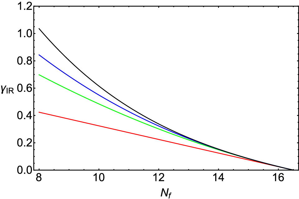
Having the four SI values $\gamma_{IR,\Delta^{p}}$ with $1\leq p\leq 4$, we can carry out a polynomial extrapolation to estimate the exact $\gamma_{IR}=\lim_{p\to\infty}\gamma_{IR,\Delta^{p}}$ for each $N_{f}$. We have investigated two such extrapolations, one of which uses all four terms and the other of which uses the three highest-order terms, i.e. $p=2,\ 3,\ 4$. These two types of extrapolations give consistent results. We report the values obtained with the second extrapolation method here. For example, for $N_{f}=12$, we obtain the fitting polynomial $\gamma_{IR,\Delta^{p},fit}=0.2048p^{-2}-0.3005p^{-1}+0.400$, from which we get $\gamma_{IR}=\lim_{p\to\infty}\gamma_{IR,\Delta^{p},fit}=0.400$ for this $N_{f}$. We list our results for $\gamma_{IR}$ as a function of $N_{f}$ from this extrapolation in Table 1. For $N_{f}$ values near the upper end of the interval $I_{IRZ}$, where $\Delta_{f}$ is small, our $\gamma_{IR,\Delta^{4}}$ and extrapolation to the exact $\gamma_{IR}$ (both of which are SI) are very close to the value of $\gamma_{IR,4\ell}$ calculated in the $\overline{\rm MS}$ scheme [12, 13] and in other schemes [16] and to the value of $\gamma_{IR,5\ell}$ in [22]. As $N_{f}$ decreases in $I_{IRZ}$ , our $\gamma_{IR,\Delta^{5}}$ and extrapolated exact $\gamma_{IR}$ become progressively larger than the corresponding values of $\gamma_{IR,n\ell}$ for $3\leq n\leq 5$. If we were to apply the same extrapolation procedure at $N_{f}=8$ (below $N_{f,b2z}$), we would get an unphysical value of $\gamma_{IR}$ slightly above 2.

An important general result concerns the monotonicity of $\gamma_{IR}$ as a function of $N_{f}$. We find that for $G={\rm SU}(N_{c})$ for general $N_{c}$ and for $R$ equal to the fundamental, adjoint, and symmetric and antisymmetric rank-2 tensor representations, the $\kappa_{p}$ for $p=1,\ 2,\ 3$ given in [23] are positive. Hence, for all of these cases, for $p=1,2,3$, $\gamma_{IR,\Delta^{p}}$ is a monotonically increasing function of $\Delta_{f}$, i.e., a monotonically decreasing function of $N_{f}$ in the range where this $\Delta_{f}$ expansion applies, which includes the interval $I_{IRZ}$. Further, our Eq. (11) shows that $\kappa_{4}>0$ $G={\rm SU}(3)$ and $R=F$, so for this case $\gamma_{IR,\Delta^{4}}$ and our extrapolated exact $\gamma_{IR}$ are also monotonically increasing functions of $\Delta_{f}$, i.e. decreasing functions of $N_{f}$, throughout $I_{IRZ}$. A plausible conjecture, based on these results, is that for $G={\rm SU}(N_{c})$ with general $N_{c}$ and for $R=F$, $\kappa_{p}>0$ for all $p\geq 1$. Assuming this conjecture is correct, then the inequality $\gamma_{IR,\Delta^{p}}\leq\gamma_{IR}$ follows (realized as a strict inequality except at $N_{f}=N_{f,b1z}$ where $\gamma_{IR}=0$). We note that $\kappa_{p}>0$ for all $p\geq 1$ in QCD with ${\cal N}=1$ supersymmetry (SQCD) [25, 23].

We next compare our results for $\gamma_{IR,\Delta^{4}}$ and extrapolation for $\gamma_{IR}$ with lattice measurements of $\gamma_{IR}$ [26]. The most extensive measurements have been carried out for $N_{f}=12$ and range from $\gamma_{IR}\sim 0.4$ to $\gamma_{IR}\simeq 0.2$ [27]-[32]. Our value $\gamma_{IR,\Delta^{4}}=0.338$ and our extrapolated $\gamma_{IR}=0.40$ are consistent with this range of lattice measurements and are somewhat higher than the five-loop value $\gamma_{IR,5\ell}=0.255$ from the conventional $\alpha$ series that we obtained in [22]. There is also consistency between our determinations of $\gamma_{IR}$ and rough estimates that $\gamma_{IR}\sim 1$ from lattice studies for $N_{f}=10$ [33] and $N_{f}=8$ [34, 35].

Combining the upper bound $\gamma_{IR}<2$ with the monotonicity of $\gamma_{IR}$, we infer that if $\gamma_{IR}$ saturates its upper bound as $N_{f}\searrow N_{f,cr}$ at the lower end of the NACP [36], then we would conclude that $8<N_{f,cr}<9$. However, we stress that it is not known if, in fact, $\gamma_{IR}$ saturates its upper bound in this way as $N_{f}\searrow N_{f,cr}$.

In contrast to $\gamma_{IR}$, the IR zero of $\beta$, $\alpha_{IR}$, is scheme-dependent. Nevertheless, one can use the $\Delta_{f}$ expansion to obtain an estimate of $\alpha_{IR}$ that is complementary to the estimate from the calculation of the zero of $\beta$ expressed as a series expansion in powers of $\alpha$. We write

We have calculated the $\tilde{a}_{n}$ for general $G$ and $R$ for $1\leq n\leq 3$. Using $b_{5}$ from [21] for $G={\rm SU}(3)$ and $R=F$, we have also calculated $\tilde{a}_{4}$ for this case, for which we find

In summary, using the recently calculated $b_{5}$ from [21], we have presented a scheme-independent calculation of $\gamma_{IR,\Delta^{4}}$ and an extrapolation to estimate the exact anomalous dimension of the fermion bilinear at the IR zero of the beta function, $\gamma_{IR}$, as a function of $N_{f}$ in a QCD-like gauge theory. We have compared the results with $n$-loop calculations obtained from power series in the coupling and with lattice measurements.

The research of T.A.R. and R.S. was supported in part by the Danish National Research Foundation grant DNRF90 to CP³-Origins at SDU and by the U.S. NSF Grant NSF-PHY-13-16617, respectively.

References

- [1] Some early works include E. C. G. Stueckelberg and A. Peterman, Helv. Phys. Acta 26, 499 (1953); M. Gell-Mann and F. Low, Phys. Rev. 95, 1300 (1954); N. N. Bogolubov and D. V. Shirkov, Doklad. Akad. Nauk SSSR 103, 391 (1955); C. G. Callan, Phys. Rev. D 2, 1541 (1970); K. Symanzik, Commun. Math. Phys. 18, 227 (1970); K. Wilson, Phys. Rev. D 3, 1818 (1971).
- [2] D. J. Gross, in R. Balian and J. Zinn-Justin, eds. Methods in Field Theory, Les Houches 1975 (North Holland, Amsterdam, 1976), p. 141.
- [3] D. J. Gross and F. Wilczek, Phys. Rev. Lett. 30, 1343 (1973); H. D. Politzer, Phys. Rev. Lett. 30, 1346 (1973); G. ’t Hooft, unpublished.
- [4] W. E. Caswell, Phys. Rev. Lett. 33, 244 (1974); D. R. T. Jones, Nucl. Phys. B 75, 531 (1974).
- [5] O. V. Tarasov, A. A. Vladimirov, and A. Yu. Zharkov, Phys. Lett. B 93, 429 (1980); S. A. Larin and J. A. M. Vermaseren, Phys. Lett. B 303, 334 (1993).
- [6] T. van Ritbergen, J. A. M. Vermaseren, and S. A. Larin, Phys. Lett. B 400, 379 (1997).
- [7] M. Czakon, Nucl. Phys. B 710, 485 (2005).
- [8] W. A. Bardeen, A. J. Buras, D. W. Duke, and T. Muta, Phys. Rev. D 18, 3998 (1978).
- [9] T. Banks and A. Zaks, Nucl. Phys. B 196, 189 (1982).
- [10] E. Gardi and M. Karliner, Nucl. Phys. B 529, 383 (1998); E. Gardi and G. Grunberg, JHEP 03, 024 (1999).
- [11] F. A. Chishtie, V. Elias, V. A. Miransky, and T. G. Steele, Prog. Theor. Phys. 104, 603 (2000).
- [12] T. A. Ryttov, R. Shrock, Phys. Rev. D 83, 056011 (2011) [arXiv:1011.4542].
- [13] C. Pica, F. Sannino, Phys. Rev. D 83, 035013 (2011) [arXiv1011.5917].
- [14] R. Shrock, Phys. Rev. D 87, 105005 (2013); R. Shrock, Phys. Rev. D 87, 116007 (2013).
- [15] Refs. [12]-[14] studied the IR zero in and resultant for general and fermion representation .
- [16] T. A. Ryttov and R. Shrock, Phys. Rev. D 86, 065032 (2012); T. A. Ryttov and R. Shrock, Phys. Rev. D 86, 085005 (2012); R. Shrock, Phys. Rev. D 88, 036003 (2013); R. Shrock, Phys. Rev. D 90, 045011 (2014); R. Shrock, Phys. Rev. D 91, 125039 (2015); G. Choi and R. Shrock, Phys. Rev. D 90, 125029 (2014); G. Choi and R. Shrock, arXiv:1607.03500; T. A. Ryttov, Phys. Rev. D 89, 016013 (2014); T. A. Ryttov, Phys. Rev. D 89, 056001 (2014); T. A. Ryttov, Phys. Rev. D 90, 056007 (2014). J. A. Gracey and R. M. Simms, Phys. Rev. D 91, 085037 (2015); P. M. Stevenson, arXiv:1607.01670.
- [17] The anomalous dimension is often denoted ; we use the more general notation here, since no mass is generated in the non-Abelian Coulomb phase.
- [18] J. A. M. Vermaseren, S. A. Larin, and T. van Ritbergen, Phys. Lett. B 405, 327 (1997).
- [19] In the conformal phase, see S. Ferrara, R. Gatto, A. F. Grillo, Phys. Rev. D 9, 3564 (1974); G. Mack, Commun. Math. Phys. 55, 1 (1977); B. Grinstein, K. Intriligator, and I. Rothstein, Phys. Lett. B 662, 367 (2008). In the phase with SSB, the dynamically generated momentum-dependent fermion mass is up to logs, and the requirement that (where Euclidean momentum) yields the same bound.
- [20] P. A. Baikov, K. G. Chetyrkin, and J. H. Kühn, JHEP 10, 076 (2014).
- [21] P. A. Baikov, K. G. Chetyrkin, and J. H. Kühn, arXiv:1606.08659.
- [22] T. A. Ryttov and R. Shrock, arXiv:1607.06866.
- [23] T. A. Ryttov, Phys. Rev. Lett., in press [arXiv:1604.00687].
- [24] Aside from , the numerators of terms in these do not have similarly simple factorizations; e.g., in , , in , , etc.
- [25] V. A. Novikov, M. A. Shifman, A. I. Vainshtein, and V. I. Zakharov, Nucl. Phys. B 229, 381, 407 (1983); Phys. Lett. B 166, 329 (1986).
- [26] See, e.g., talks in the CP3 Workshop at http://cp3-origins.dk/events/meetings/mass2013; Lattice-2014 at https://www.bnl.gov/lattice2014; SCGT15 at http://www.kmi.nagoya-u.ac.jp/workshop/SCGT15; and Lattice-2015 at http://www.aics.riken.jp/sympo/lattice2015. We note that there is not yet a consensus among all lattice groups concerning the value of for this SU(3) theory.
- [27] T. Appelquist et al. (LSD Collab.), Phys. Rev. D 84, 054501 (2011).
- [28] T. DeGrand, Phys. Rev. D 84, 116901 (2011).
- [29] Y. Aoki et al. (LatKMI Collab.), Phys. Rev. D 86, 054506 (2012).
- [30] A. Hasenfratz, A. Cheng, G. Petropoulos, and D. Schaich, in Proc. Lattice-2012 [arXiv:1207.7162]; and A. Hasenfratz, A. Cheng, G. Petropoulos, and D. Schaich, in Proc. Lattice-2013 [arXiv:1310.1124].
- [31] M. P. Lombardo, K. Miura, T. J. Nunes da Silva, and E. Pallante, JHEP 12, 183 (2014) [arXiv:1410.0298].
- [32] Z. Fodor, K. Holland, J. Kuti, D. Nogradi, C. Schroeder, and C.H. Wong, in Proc. Lattice-2012 [arXiv:1211.4238]; Z. Fodor, K. Holland, J. Kuti, S. Mondal, D. Nogradi, and C. H. Wong, arXiv:1607.06121.
- [33] T. Appelquist et al. (LSD Collab.), arXiv:1204.6000.
- [34] Y. Aoki et al. (LatKMI Collab.), Phys. Rev. D 87, 094511 (2013); Y. Aoki et al. (LatKMI Collab.), Phys. Rev. D 89, 111502 (2014).
- [35] T. Appelquist et al. (LSD Collab.), Phys. Rev. D 90, 114502 (2014).
- [36] In SQCD, the upper bound on is in the NACP, and does saturate this upper bound as the the number of pairs of chiral superfields and decreases toward the lower end of the NACP.