跳到论文正文
W Papers独立论文阅读器 arXiv:1607.08727 论文正文 计算阅读时间 · 0%
引用这篇论文根据当前论文元数据生成,正式投稿前建议核对。


License: arXiv.org perpetual non-exclusive license
arXiv:1607.08727v2 [hep-ph] 01 Mar 2018

Renormalization-group analysis of B→πB\to\pi form factors with BB-meson Light-Cone Sum Rules
Yue-Long Shena, Yan-Bing Weib and Cai-Dian Lüb
a College of Information Science and Engineering, Ocean University of China, Qingdao, Shandong 266100, P.R. China
bInstitute of High Energy Physics, CAS, P.O. Box 918(4), Beijing 100049, P.R. China

Abstract

Within the framework of the BB-meson light-cone sum rules, we review the calculation of radiative corrections to the three B→πB\to\pi transition form factors at leading power in Λ/mb\Lambda/m_{b}. To resum large logarithmic terms, we perform the complete renormalization-group evolution of the correlation function. We employ the integral transformation which diagonalizes evolution equations of the jet function and the BB-meson light-cone distribution amplitude to solve these evolution equations, and obtain renormalization-group improved sum rules for the B→πB\to\pi form factors. Results of the form factors are extrapolated to the whole physical q2q^{2} region, and are compared with that of other approaches. The effect of BB-meson three-particle light-cone distribution amplitudes, which will contribute to the form factors at next-to-leading power in Λ/mb\Lambda/m_{b} at tree level, is not considered in this paper.

1 INTRODUCTION

The knowledge of the heavy-to-light transition form factors is of great importance because it is crucial for the determination of parameters of the standard model, and for the understanding of strong interaction dynamics. The B→πB\to\pi transition form factors, which are closely related to the CKM matrix element |Vu​b||V_{ub}|, have been extensively studied in the literature. Because of the appearance of the endpoint singularity in the factorization of the heavy-to-light form factors, the form factors are regarded, in many approaches, as dominated by long-distance QCD dynamics and can be calculated only with non-perturbative methods, such as Lattice QCD, (Light-Cone) QCD Sum Rules, et al. In [1, 2, 3, 4, 5, 6, 7, 8], the light-cone sum rules (LCSR) with pion light-cone distribution amplitudes (LCDAs) has been employed to study the B→πB\to\pi form factors, and next-to-leading-order (NLO) corrections to the twist-2 and the twist-3 terms as well as renormalization-group (RG) evolution effects [9] have been considered. In this paper, we use the LCSR with BB-meson LCDAs [10, 11] to calculate the B→πB\to\pi form factors. The BB-meson LCSR has also been established independently in the framework of the soft-collinear effective theory (SCET) [12, 13], where jet functions encoding the “hard-collinear” dynamics have been calculated up to 𝒪⁡(αs){\cal O}(\alpha_{s}) [14, 15]. An alternative approach to analyse NLO corrections to the sum rules is suggested in [16], where the “method of regions” [17] was adopted to compute the vector form factor fB​π+​(q2)f_{B\pi}^{+}(q^{2}) and the scalar form factor fB​π0​(q2)f_{B\pi}^{0}(q^{2}) defined below

⟨π⁡(p)​|u¯​γμ​b|​B¯​(pB)⟩\displaystyle\langle\pi(p)|\bar{u}\gamma^{\mu}b|\bar{B}(p_{B})\rangle =\displaystyle= fB​π+​(q2)​[pB+p−mB2−mπ2q2​q]μ+fB​π0​(q2)​mB2−mπ2q2​qμ.\displaystyle f_{B\pi}^{+}(q^{2})\,\left[p_{B}+p-\frac{m_{B}^{2}-m_{\pi}^{2}}{q^{2}}q\right]^{\mu}+f_{B\pi}^{0}(q^{2})\,\frac{m_{B}^{2}-m_{\pi}^{2}}{q^{2}}q^{\mu}\,. (1)

Results of the BB-meson LCSR were shown to be consistent with that of the SCET sum rules. There is another B→πB\rightarrow\pi transition form factor which is defined by the tensor current:

⟨π⁡(p)|q¯​σμ​ν​qν​b|B⁡(pB)⟩\displaystyle\langle\pi(p)|\bar{q}\sigma^{\mu\nu}q_{\nu}b|B(p_{B})\rangle =\displaystyle= i​fB​πT​(q2)mB+mπ​[(pB+p)μ​q2−(mB2−mπ2)​qμ],\displaystyle\frac{if_{B\pi}^{T}(q^{2})}{m_{B}+m_{\pi}}[(p_{B}+p)^{\mu}q^{2}-(m_{B}^{2}-m_{\pi}^{2})q^{\mu}]\,, (2)

and this form factor was not computed in [16]. In the heavy-quark limit and at leading order in αs\alpha_{s}, the three independent form factors are proportional to one universal form factor at large recoil. If loop corrections are included, differences between the three form factors appear. The hard-spectator-scattering part can be factorized into a convolution of the perturbative function and the LCDAs of hadrons (BB meson and pion) using the QCD factorization approach [18]. Both QCD corrections to the universal form factor and to symmetry-breaking hard-spectator interactions have been calculated in [14, 15]. Using the method of regions, QCD corrections to the symmetry-conserving (universal) form factor and the symmetry-breaking part of the form factors are computed simultaneously.

The first step towards using the method of regions is identifying leading regions which are in principle determined by the analytic structure of the Feynman diagram [19]. Usually leading regions are closely related to momentum modes of external lines. In this work, there are three momentum modes from external lines, namely the hard (bb-quark), the hard-collinear (interpolating current of pion) and the soft (light-spectator quark) modes. Thus, three momentum regions with scaling behaviors

Pμ≡(n⋅P,n¯⋅P,P⟂),\displaystyle P_{\mu}\equiv(n\cdot P\,,\bar{n}\cdot P\,,P_{\perp})\,, Ph,μ∼𝒪⁡(1,1,1),\displaystyle P_{h\,,\,\mu}\sim{\cal O}(1,1,1)\,,
Ph​c,μ∼𝒪⁡(1,λ,λ1/2),\displaystyle P_{hc\,,\,\mu}\sim{\cal O}(1,\lambda,\lambda^{1/2})\,, Ps,μ∼𝒪⁡(λ,λ,λ),\displaystyle P_{s\,,\,\mu}\sim{\cal O}(\lambda,\lambda,\lambda)\,, (3)

can contribute to the correlation function at leading power in λ\lambda, where λ∼Λ/mb\lambda\sim{\Lambda/m_{b}} and nμn_{\mu} and n¯μ\bar{n}_{\mu} are light-cone vectors, satisfying n2=n¯2=0n^{2}=\bar{n}^{2}=0 and n⋅n¯=2n\cdot\bar{n}=2. In our calculation, only these three regions give leading-power contributions to the correlation function, which is in agreement with the general analysis. The momentum of the fast-moving pion is chosen to be along the n¯\bar{n} direction. This momentum is also chosen to be hard-collinear and in the Euclidean region (p2<0p^{2}<0) to ensure the light-cone operator-product expansion (OPE) of the correlation function [10, 11]. The method of regions provides us a natural way to perform the factorization of the correlation function because contributions of different momentum regions are considered individually. It has been shown that the correlation function can be factorized into the convolution of the hard function, the jet function and the BB-meson LCDA which describe dynamics of the hard, the hard-collinear and the soft regions, respectively. This procedure is equivalent to the two-step matching in the SCET where the hard (jet) function corresponds to the matching coefficient of SCETI{\rm SCET_{I}} (SCETII{\rm SCET_{II}}) [20, 21].

The correlation function is factorization-scale independent, thus the scale dependence of the hard function, the BB-meson static decay constant, the jet function and the BB-meson LCDA must be cancelled, which has been shown at one-loop level [15, 16]. At present, there is still no complete analysis of RG evolutions of all of the relevant functions. In [16], RG evolutions of the hard function and the BB-meson decay constant were performed. The factorization scale in that paper was chosen to be about 1.51.5GeV, which is a typical hard-collinear scale. This choice is phenomenologically reasonable as the hard-collinear scale is not far from the non-perturbative scale. RG evolutions of the jet function and the BB-meson LCDA are non-trivial since anomalous dimensions of these two functions are complicated. But on the conceptual side, a complete RG analysis is necessary.

BB-meson LCDAs ϕB−​(ω)\phi_{B}^{-}(\omega) and ϕB+​(ω)\phi_{B}^{+}(\omega) are fundamental inputs of the BB-meson LCSR. They are defined by the matrix element [22]

⟨0|d¯β​(τ​n¯)​[τ​n¯,0]​bα​(0)|B¯​(p+q)⟩=−i​f~B​(μ)​mB4​{1+v̸2​[2​ϕ~B+​(τ)+(ϕ~B−​(τ)−ϕ~B+​(τ))​n̸]​γ5}α​β,\displaystyle\langle 0|\bar{d}_{\beta}(\tau\,\bar{n})\,[\tau\bar{n},0]\,b_{\alpha}(0)|\bar{B}(p+q)\rangle=-\frac{i\tilde{f}_{B}(\mu)\,m_{B}}{4}\bigg\{\frac{1+\!\not v}{2}\,\left[2\,\tilde{\phi}_{B}^{+}(\tau)+\left(\tilde{\phi}_{B}^{-}(\tau)-\tilde{\phi}_{B}^{+}(\tau)\right)\!\not n\right]\,\gamma_{5}\bigg\}_{\alpha\beta}\,, (4)

where [τ​n¯,0][\tau\bar{n},0] is the Wilson line along the n¯\bar{n} direction, vv and f~B​(μ)\tilde{f}_{B}(\mu) are the BB-meson velocity vector and the BB-meson static decay constant, respectively. The Fourier transformation of ϕ~B±​(τ)\tilde{\phi}_{B}^{\pm}(\tau) leads to

ϕB±​(ω)=∫−∞+∞d​τ2​π​ei​ω​τ​ϕ~B±​(τ−i​0).\displaystyle\phi_{B}^{\pm}(\omega)=\int_{-\infty}^{+\infty}\,\frac{d\,\tau}{2\,\pi}\,e^{i\,\omega\,\tau}\,\tilde{\phi}_{B}^{\pm}(\tau-i0)\,. (5)

The scale dependence of ϕB±​(ω)\phi_{B}^{\pm}(\omega) has been studied extensively [23, 24]. ϕB±​(ω)\phi_{B}^{\pm}(\omega) obeys the RG equation with the anomalous dimension being the Lange-Neubert kernel [23]. It is difficult to solve the Lange-Neubert equation in the momentum space. With the eigenfunction of the Lange-Neubert kernel found in [24], the RG equation of ϕB±​(ω)\phi_{B}^{\pm}(\omega) can be diagonalized and readily solved. The RG equation of the jet function can be simplified in the same way since the scale dependence of the jet function should be partly cancelled by that of the BB-meson LCDA.

In this work, we only consider leading-power contributions of the B→πB\to\pi form factors. BB-meson three-particle LCDAs can give subleading-power contributions to the form factors at leading order (LO) in αs\alpha_{s} and give leading-power contributions at NLO [25]. Numerically, the subleading-power correction from three-particle LCDAs is only a few percent of the leading-power contribution from two-particle LCDAs [10]. Feynman diagrams related to three-particle LCDAs can be seen in [16]. The calculation of effects of three-particle LCDAs is expected to be rather complicated, and RG equations of the three-particle LCDAs are not completely available so far. Thus we leave this part for the future work.

This paper is arranged as follows. In Section 2 we briefly review the calculation of the B→πB\to\pi form factors at NLO and emphasize symmetry-breaking effects of these form factors. Then, the RG evolution of the correlation function is shown in details in the following section. In Section 4 we turn to the numerical analysis of the RG improved form factors. Concluding discussions are presented in Section 5. The Appendix includes two parts, the jet function in the “dual” space and dispersion integrals used in the sum rules.

2 THE B→πB\to\pi FORM FACTORS WITH B-MESON LCSRs

In order to derive the sum rules for the B→πB\to\pi transition form factors, we start with the correlation function

Πμ​(p,q)\displaystyle\Pi^{\mu}(p,q) =\displaystyle= i​∫d4​x​ei​p⋅x​⟨0|T⁡{d¯​(x)/n​γ5​u​(x),u¯​(0)​Γμ​b​(0)}|B¯​(PB)⟩,\displaystyle i\int d^{4}x~e^{ip\cdot x}\langle 0|T\left\{\bar{d}(x)/\!\!\!n\gamma_{5}u(x),\bar{u}(0)\Gamma^{\mu}b(0)\right\}|\bar{B}(P_{B})\rangle\,, (6)

where Γμ=γμ​(σμ​ν​qν)\Gamma^{\mu}=\gamma^{\mu}(\sigma^{\mu\nu}q_{\nu}) denoting the vector (tensor) current. According to the Lorentz-structure analysis, the correlation function is parameterized as Πμ​(n⋅p,n¯⋅p)=Πn​(n⋅p,n¯⋅p)​nμ+Πn¯​(n⋅p,n¯⋅p)​n¯μ\Pi^{\mu}(n\cdot p,\bar{n}\cdot p)=\Pi_{n}(n\cdot p,\bar{n}\cdot p)\,n^{\mu}+{\Pi}_{\bar{n}}(n\cdot p,\bar{n}\cdot p)\,\bar{n}^{\mu}\, for the vector current, and Πμ​(p,q)=ΠT​(n⋅p,n¯⋅p)​ϵ∥μ​ν​qν\Pi^{\mu}(p,q)=\Pi_{\rm T}(n\cdot p,\bar{n}\cdot p)\epsilon_{\parallel}^{\mu\nu}q_{\nu} for the tensor current, where the anti-symmetric tensor ϵ∥μ​ν=(nμ​n¯ν−nν​n¯μ)/2\epsilon_{\parallel}^{\mu\nu}=(n^{\mu}\bar{n}^{\nu}-n^{\nu}\bar{n}^{\mu})/2. We work in the rest frame of the BB meson and the power-counting rule of the pion momentum reads

n⋅p∼𝒪⁡(mb),n¯⋅p∼𝒪⁡(Λ).\displaystyle n\cdot p\sim{\cal O}(m_{b}),\,\,\,\,\,\bar{n}\cdot p\sim{\cal O}(\Lambda). (7)

In Euclidean region (n¯⋅p<0\bar{n}\cdot p<0) the light-cone OPE is employed to calculate the correlation function. Tree-level results are written as

Πn¯(0)​(n⋅p,n¯⋅p)\displaystyle{\Pi}^{(0)}_{\bar{n}}(n\cdot p,\bar{n}\cdot p) =\displaystyle= ΠT(0)​(n⋅p,n¯⋅p)=f~B​(μ)​mB​∫0∞d​ω′​ϕB−​(ω′)ω′−n¯⋅p−i​ 0,\displaystyle\Pi^{(0)}_{\rm T}(n\cdot p,\bar{n}\cdot p)=\tilde{f}_{B}(\mu)\,m_{B}\,\int_{0}^{\infty}d\omega^{\prime}\,\frac{\phi_{B}^{-}(\omega^{\prime})}{\omega^{\prime}-\bar{n}\cdot p-i\,0}\,,
Πn(0)​(n⋅p,n¯⋅p)\displaystyle\Pi^{(0)}_{n}(n\cdot p,\bar{n}\cdot p) =\displaystyle= 0.\displaystyle 0\,. (8)

The correlation function can also be expressed in terms of the B→πB\to\pi form factors and the pion decay constant. For instance

ΠT​(p,q)=i​(n⋅p)2​fπ​fB​πT​(q2)​mB(mπ2−p2)​(mB+mπ)+∫ωs∞d​ω​ρh​(ω)ω−n¯⋅p−i​ϵ,\displaystyle\Pi_{\rm T}(p,q)=\frac{i(n\cdot p)^{2}f_{\pi}f^{T}_{B\pi}(q^{2})m_{B}}{(m_{\pi}^{2}-p^{2})(m_{B}+m_{\pi})}+\int_{\omega_{s}}^{\infty}d\omega\frac{\rho_{h}(\omega)}{\omega-\bar{n}\cdot p-i\epsilon}, (9)

where ρh​(ω)\rho_{h}(\omega) represents the contribution of excited and continuum states which have the same quantum numbers as pion. The form factors are extracted by matching the partonic and the hadronic representations of the correlation function. After performing the Borel transformation which suppresses the contribution of excited and continuum states, we obtain the sum rules for the tensor form factor at LO

fB​πT(q2)=fB​(mB+mπ)n⋅p​fπemπ2/(n⋅p​ωM)∫0ωsdωe−ω/ωMϕ−B(ω).\displaystyle f^{T}_{B\pi}(q^{2})=\frac{f_{B}(m_{B}+m_{\pi})}{n\cdot pf_{\pi}}e^{m_{\pi}^{2}/(n\cdot p\omega_{M})}\int^{\omega_{s}}_{0}d\omega e^{-\omega/\omega_{M}}\phi^{B}_{-}(\omega). (10)

Large-recoil symmetry relations [18] indicate:

fB​π+​(q2)=mBn⋅p​fB​π0​(q2)=mBmB+mπ​fB​πT​(q2)=ξ⁡(n⋅p),\displaystyle f^{+}_{B\pi}(q^{2})={m_{B}\over n\cdot p}f^{0}_{B\pi}(q^{2})=\frac{m_{B}}{m_{B}+m_{\pi}}f^{T}_{B\pi}(q^{2})=\xi(n\cdot p), (11)

where ξ⁡(n⋅p)\xi(n\cdot p) is the Isgur-Wise function. These symmetry relations will be broken by QCD corrections.

Refer to caption

(a)          (b)         (c)          (d)

Figure 1: Diagrammatic representation of the correlation function Πμ​(n⋅p,n¯⋅p)\Pi^{\mu}(n\cdot p,\bar{n}\cdot p) at next-to-leading order in αs\alpha_{s}.
Refer to caption

(a)              (b)             (c)

Figure 2: One-loop-level diagrams of the BB-meson DA Φb​u¯α​β​(ω′)\Phi_{b\bar{u}}^{\alpha\beta}(\omega^{\prime}).

The method of computing radiative corrections to the correlation function has been introduced in [16]. Adopting the diagrammatic factorization method [26], the hard-scattering kernel at NLO is determined by the matching condition

Φb​d¯(0)⊗T(1)=Πb​d¯(1)−Φb​d¯(1)⊗T(0),\displaystyle\Phi_{b\bar{d}}^{(0)}\otimes T^{(1)}=\Pi_{b\bar{d}}^{(1)}-\Phi_{b\bar{d}}^{(1)}\otimes T^{(0)}\,, (12)

where the first and the second terms on the right-hand side of the equation correspond to full-theory diagrams (Fig.1) and effective diagrams (Fig.2), respectively. The Lorentz index “μ\mu” is suppressed in this equation. The definition of Φb​d¯(0,1)\Phi_{b\bar{d}}^{(0,1)} can be seen in [16]. It has been proved that soft dynamics are completely cancelled between Πb​d¯(1)\Pi_{b\bar{d}}^{(1)} and Φb​d¯(1)⊗T(0)\Phi_{b\bar{d}}^{(1)}\otimes T^{(0)}. Thus the hard-scattering kernel TT contains only contributions from hard and hard-collinear regions at leading power in λ\lambda, with the hard-region and the hard-collinear-region contributions corresponding to the hard function and the jet function, respectively. The correlation function is factorized as:

Πa​(p,q)\displaystyle\Pi_{a}(p,q) =\displaystyle= f~B(μ)mB∑k=±Ca(k)(n⋅p,μ)∫0∞d​ωω−n¯⋅pJa(k)(μ2n⋅p​ω,ωn¯⋅p)ϕBk(ω,μ),\displaystyle\tilde{f}_{B}(\mu)\,m_{B}\sum\limits_{k=\pm}\,C_{a}^{(k)}(n\cdot p,\mu)\,\int_{0}^{\infty}{d\omega\over\omega-\bar{n}\cdot p}~J_{a}^{(k)}\left({\mu^{2}\over n\cdot p\,\omega},{\omega\over\bar{n}\cdot p}\right)\,\phi_{B}^{k}(\omega,\mu),\, (13)

where a=n,n¯,Ta=n,\,{\bar{n}},\,T. Results of Cn,Cn¯,Jn,Jn¯C_{n},\,C_{\bar{n}},\,J_{n},\,J_{\bar{n}} have been given in [16]. CTC_{T} and JTJ_{T} can be calculated following the same method. Nevertheless, using symmetry relations between the form factors, we are able to obtain CTC_{T} and JTJ_{T} without repeating the calculation. Symmetry relations in Eq.(11) are broken by loop corrections. The difference between CTC_{T} (JTJ_{T}) and Cn¯C_{\bar{n}} (Jn¯J_{\bar{n}}) comes from the symmetry-breaking effect. At one-loop level large-recoil relations can be written as [18]:

fB​π0\displaystyle f^{0}_{B\pi} =\displaystyle= fB​π+​[1+αs4​π​(2+2​rr¯​ln⁡r)]​r+αs4​π​Δ​f0,\displaystyle f^{+}_{B\pi}[1+{\alpha_{s}\over 4\pi}(2+{2r\over\bar{r}}\ln r)]r+{\alpha_{s}\over 4\pi}\Delta f_{0},
fB​πT\displaystyle f^{T}_{B\pi} =\displaystyle= fB​π+​[1+αs4​π​(2​ln⁡mb2μ2−2​rr¯​ln⁡r)]​r+αs4​π​Δ​fT,\displaystyle f^{+}_{B\pi}[1+{\alpha_{s}\over 4\pi}(2\ln{m_{b}^{2}\over\mu^{2}}-{2r\over\bar{r}}\ln r)]r+{\alpha_{s}\over 4\pi}\Delta f_{T}, (14)

where r=n⋅p/mbr=n\cdot p/m_{b}. The first line of above equations has been confirmed in [14, 16].

The first kind of symmetry-breaking effects, which is shown in the square brackets of Eq.(14), arises from the hard function of weak-vertex correction Fig.1(a). The weak tensor current u¯​(0)​i​σμ​ν​qν​b​(0)\bar{u}(0)i\sigma^{\mu\nu}q_{\nu}b(0) is not a conserved current, thus there exists operator-renormalization contribution to the correction function of the tensor current. This contribution produces an additional term to the hard function

CT(−)​(n⋅p,μ,ν)=CT(−)​(n⋅p,μ)+δ​CT(−)​(n⋅p,μ,ν),\displaystyle C^{(-)}_{T}(n\cdot p,\mu,\nu)=C^{(-)}_{T}(n\cdot p,\mu)+\delta C^{(-)}_{T}(n\cdot p,\mu,\nu), (15)

where ν\nu is the renomalization scale. δ​CT(−)​(n⋅p,μ,ν)\delta C^{(-)}_{T}(n\cdot p,\mu,\nu) corresponds to the ln⁡mb2μ2\ln{m_{b}^{2}\over\mu^{2}} term (μ\mu should be changed to ν\nu) in Eq.(14). Inserting the hard function of fB​π+f^{+}_{B\pi} [16] into Eq.(15), we obtain

CT(−)​(n⋅p,μ,ν)\displaystyle C^{(-)}_{T}(n\cdot p,\mu,\nu) =\displaystyle= 1−αs​CF4​π[2lnνmb+2ln2μmb−(4lnr−5)lnμmb\displaystyle 1-\frac{\alpha_{s}\,C_{F}}{4\,\pi}\,\bigg[2\ln\frac{\nu}{m_{b}}+2\ln^{2}{\mu\over m_{b}}-(4\ln r-5)\ln{\mu\over m_{b}} (16)
+2ln2r+2Li2(r¯)−4​r−2r−1lnr+π212+6].\displaystyle+2\ln^{2}r+2{\rm Li_{2}}\left(\bar{r}\right)-{4r-2\over r-1}\,\ln r+{\pi^{2}\over 12}+6\bigg].

The second kind of symmetry-breaking effects Δ​fT\Delta f_{T} which corresponds to Fig.1(b,c), comes from the “hard spectator” contribution in the QCD factorization. Since only the hard-collinear region contributes to Fig.1(b,c) at leading power in λ\lambda, Δ​fT\Delta f_{T} is related to jet functions. The jet function JT(−)J_{T}^{(-)}, which equals Jn¯(−)J_{\bar{n}}^{(-)}, is the symmetry-conserving term. Only JT(+)J_{T}^{(+)} corresponds to the symmetry-breaking effect. Comparing Δ​fT\Delta f_{T} with Δ​f0\Delta f_{0}, and employing the result of Jn,n¯(+)J^{(+)}_{n,\bar{n}}, we find

JT(+)\displaystyle J_{T}^{(+)} =\displaystyle= −αs​CF4​π​(1+r)​(1+1η)​ln⁡(1+η),\displaystyle-\frac{\alpha_{s}\,C_{F}}{4\,\pi}(1+r)(1+\frac{1}{\eta})\ln(1+\eta), (17)

where η=−ω/n¯⋅p\eta=-\omega/\bar{n}\cdot p.

3 RG evolution

The hard and the jet functions contain logarithmic terms such as ln2⁡μn⋅p\ln^{2}\frac{\mu}{n\cdot p} and ln⁡μn⋅p\ln\frac{\mu}{n\cdot p}, which become large when the factorization scale μ\mu is much smaller than n⋅pn\cdot p. The RG equation approach can be used to resum large logarithms to all orders in αs\alpha_{s}. In the following, we will present details of the RG evolution of ΠT​(n⋅p)\Pi_{\rm T}(n\cdot p), and the approach can be easily generalized to Πn​(n⋅p)\Pi_{n}(n\cdot p) and Πn¯​(n⋅p)\Pi_{\bar{n}}(n\cdot p).

Eq.(16) contains the operator renormalization of the tensor current, so we need to perform evolutions both to the renormalization and the factorization scales. RG equations governing the renormalization-scale and the factorization-scale dependence are given by

dd​ln⁡ν​CT(−)​(n⋅p,μ,ν)\displaystyle{d\over d\ln\nu}{C}^{(-)}_{T}(n\cdot p,\mu,\nu) =\displaystyle= γT​(αs)​CT(−)​(n⋅p,μ,ν),\displaystyle\gamma_{T}(\alpha_{s}){C}^{(-)}_{T}(n\cdot p,\mu,\nu)\,,
dd​ln⁡μ​CT(−)​(n⋅p,μ,ν)\displaystyle{d\over d\ln\mu}{C}_{T}^{(-)}(n\cdot p,\mu,\nu) =\displaystyle= ΓC​(αs)​CT(−)​(n⋅p,μ,ν),\displaystyle\Gamma_{C}(\alpha_{s}){C}^{(-)}_{T}(n\cdot p,\mu,\nu)\,, (18)

where

ΓC​(αs)=−Γcusp​(αs)​ln⁡μn⋅p+γh​(αs).\displaystyle\Gamma_{C}(\alpha_{s})=-\Gamma_{\rm cusp}(\alpha_{s})\ln{\mu\over n\cdot p}+\gamma_{h}(\alpha_{s}). (19)

Solutions to Eq.(18) are written by

CT(−)​(n⋅p,μ,ν)\displaystyle{C}^{(-)}_{T}(n\cdot p,\mu,\nu) =\displaystyle= exp⁡[∫αs​(mb)αs​(ν)d​αs​γT​(αs)β⁡(αs)]​CT(−)​(n⋅p,μ,mb)\displaystyle\exp\bigg[\int^{\alpha_{s}(\nu)}_{\alpha_{s}(m_{b})}d\alpha_{s}\frac{\gamma_{T}(\alpha_{s})}{\beta(\alpha_{s})}\bigg]{C}^{(-)}_{T}(n\cdot p,\mu,m_{b})\,
CT(−)​(n⋅p,μ,mb)\displaystyle{C}_{T}^{(-)}(n\cdot p,\mu,m_{b}) =\displaystyle= exp⁡{∫αs​(μh)αs​(μ)d​αs​[γh​(αs)β⁡(αs)+Γcusp​(αs)β⁡(αs)​(ln⁡n⋅pμh−∫αs​(μh)αsd​αs′β⁡(αs′))]}\displaystyle\exp\bigg\{\int^{\alpha_{s}(\mu)}_{\alpha_{s}(\mu_{h})}d\alpha_{s}\bigg[\frac{\gamma_{h}(\alpha_{s})}{\beta(\alpha_{s})}+\frac{\Gamma_{\rm cusp}(\alpha_{s})}{\beta(\alpha_{s})}\bigg(\ln{n\cdot p\over\mu_{h}}-\int^{\alpha_{s}}_{\alpha_{s}(\mu_{h})}\frac{d\alpha^{\prime}_{s}}{\beta(\alpha^{\prime}_{s})}\bigg)\bigg]\bigg\}\, (20)
×\displaystyle\times CT(−)​(n⋅p,μh,mb).\displaystyle{C}_{T}^{(-)}(n\cdot p,\mu_{h},m_{b})\,.

As the hard function has been calculated at one-loop level, evolution functions of the hard function are also required to be expanded to 𝒪⁡(αs){\cal O}(\alpha_{s}). The beta function appearing in Eq.(20) reads

β⁡(αs)\displaystyle\beta(\alpha_{s}) =\displaystyle= −2αs∑n=0βn(αs4​π)n+1,\displaystyle-2\alpha_{s}\sum_{n=0}\beta_{n}{\,({\alpha_{s}\over 4\pi})^{n+1}}\,, (21)

thus anomalous dimensions γh\gamma_{h} and γT\gamma_{T} need to be expanded to two-loop level:

γh​(αs)\displaystyle\gamma_{h}(\alpha_{s}) =\displaystyle= αs​CF4​π​[γh(0)+(αs4​π)​γh(1)+…],\displaystyle{\alpha_{s}\,C_{F}\over 4\pi}\,\left[\gamma_{h}^{(0)}+\left({\alpha_{s}\over 4\pi}\right)\,\gamma_{h}^{(1)}+...\right]\,,
γT​(αs)\displaystyle\gamma_{T}(\alpha_{s}) =\displaystyle= αs​CF4​π​[−2+αs4​π​(19​CF−2579​CA+529​nf′​TF)+…],\displaystyle{\alpha_{s}\,C_{F}\over 4\pi}\,\left[-2+{\alpha_{s}\over 4\pi}\left(19C_{F}-\frac{257}{9}C_{A}+\frac{52}{9}n^{\prime}_{f}T_{F}\right)+...\right], (22)

where nf′n^{\prime}_{f} is the number of the active quark flavors. While the cusp anomalous dimension Γcusp​(αs)\Gamma_{\rm cusp}(\alpha_{s}) should be expanded to three-loop level:

Γcusp​(αs)\displaystyle\Gamma_{\rm cusp}(\alpha_{s}) =\displaystyle= αs​CF4​π​[Γcusp(0)+(αs4​π)​Γcusp(1)+(αs4​π)2​Γcusp(2)+…],\displaystyle{\alpha_{s}\,C_{F}\over 4\pi}\,\left[\Gamma_{\rm cusp}^{(0)}+\left({\alpha_{s}\over 4\pi}\right)\,\Gamma_{\rm cusp}^{(1)}+\left({\alpha_{s}\over 4\pi}\right)^{2}\,\Gamma_{\rm cusp}^{(2)}+...\right]\,, (23)

since the factor ∫αs​(μh)αsd​αs′/β⁡(αs′)\int^{\alpha_{s}}_{\alpha_{s}(\mu_{h})}d\alpha^{\prime}_{s}/\beta(\alpha^{\prime}_{s}) starts at 𝒪⁡(αs−1)\mathcal{O}(\alpha^{-1}_{s}).

Note that the ν\nu dependence of the form factor must be cancelled by that of the Wilson coefficient of tensor current. For phenomenological applications, this renormalization scale can be fixed at ν=mb\nu=m_{b}. Then the corresponding evolution kernel reduces to 1, and the Wilson coefficient should be evolved to mbm_{b}. We rewrite the second equation of Eq.(20) as

CT(−)​(n⋅p,μ)\displaystyle{C}_{T}^{(-)}(n\cdot p,\mu) =\displaystyle= U1​(n⋅p,μh,μ)​CT(−)​(n⋅p,μh),\displaystyle U_{1}(n\cdot p,\mu_{h},\mu)\,{C}_{T}^{(-)}(n\cdot p,\mu_{h})\,, (24)

where the specific expression of U1​(n⋅p,μh,μ)U_{1}(n\cdot p,\mu_{h},\mu) at 𝒪⁡(αs){\cal O}(\alpha_{s}) can be found in the appendix of [27].

RG equations of the jet function and the BB-meson LCDA have following forms

dd​ln⁡μ​JT(−)​(μ2n⋅p​ω,ωn¯⋅p)=[Γcusp​(αs)​ln⁡μ2n⋅p​ω]​JT(−)​(μ2n⋅p​ω,ωn¯⋅p)\displaystyle{d\over d\ln\mu}{J}_{T}^{(-)}\left({\mu^{2}\over n\cdot p\,\omega},{\omega\over\bar{n}\cdot p}\right)=\left[\Gamma_{\rm cusp}(\alpha_{s})\ln{\mu^{2}\over n\cdot p\,\omega}\right]{J}_{T}^{(-)}\left({\mu^{2}\over n\cdot p\,\omega},{\omega\over\bar{n}\cdot p}\right)
+∫0∞dω′ωΓ(ω,ω′,μ)JT(−)(μ2n⋅p​ω′,ω′n¯⋅p),\displaystyle\hskip 85.35826pt+\,\int_{0}^{\infty}\,d\omega^{\prime}\,\omega\,\,\Gamma(\omega,\omega^{\prime},\mu)\,\,{J}_{T}^{(-)}\left({\mu^{2}\over n\cdot p\,\omega^{\prime}},{\omega^{\prime}\over\bar{n}\cdot p}\right)\,, (25)
dd​ln⁡μ​ϕB−​(ω,μ)=−[Γcusp​(αs)​ln⁡μω+γ+​(αs)]​ϕB−​(ω,μ)\displaystyle{d\over d\ln\mu}\phi_{B}^{-}(\omega,\mu)=-\left[\Gamma_{\rm cusp}(\alpha_{s})\ln{\mu\over\omega}+\gamma_{+}(\alpha_{s})\right]\phi_{B}^{-}(\omega,\mu)
−∫0∞dω′ωΓ(ω,ω′,μ)ϕB−(ω′,μ).\displaystyle\hskip 99.58464pt-\int_{0}^{\infty}\,d\omega^{\prime}\,\omega\,\,\Gamma(\omega,\omega^{\prime},\mu)\,\,\phi_{B}^{-}(\omega^{\prime},\mu)\,. (26)

These evolution kernels are non-diagonal. It is thus difficult to solve above RG equations in the momentum space. An alternative method was suggested in [24], where the LN kernel can be diagonalized by translating to the “dual” space. It was found in [28] that the basis of the dual space is the eigenfunction of the generator of special conformal transformations. The specific form of the transformation can be written by:

ρB−​(ω′,μ)=∫0∞d​ωω′​J0​(2​ωω′)​ϕB−​(ω,μ).\displaystyle\rho_{B}^{-}(\omega^{\prime},\mu)=\int^{\infty}_{0}\frac{d\omega}{\omega^{\prime}}J_{0}(2\sqrt{\frac{\omega}{\omega^{\prime}}})\phi_{B}^{-}(\omega,\mu). (27)

The dual-space LCDA ρB−​(ω′,μ)\rho_{B}^{-}(\omega^{\prime},\mu) satisfies a simpler RG equation

dd​ln⁡μ​ρB−​(ω′,μ)=Γρ​(μ)​ρB−​(ω′,μ),\displaystyle{d\over d\ln\mu}\rho_{B}^{-}(\omega^{\prime},\mu)=\Gamma_{\rho}(\mu)\rho_{B}^{-}(\omega^{\prime},\mu)\,, (28)

where Γρ​(μ)=−Γcusp​(αs)​ln⁡μω^′−γ+​(αs)\Gamma_{\rho}(\mu)=-\Gamma_{\rm cusp}(\alpha_{s})\ln{\mu\over\hat{\omega}^{\prime}}-\gamma_{+}(\alpha_{s}), and ω^′=e−2​γE​ω′\hat{\omega}^{\prime}=e^{-2\gamma_{E}}{\omega}^{\prime}. Solving the RG equation of ρB−​(μ)\rho^{-}_{B}(\mu), one has

ρB−​(ω′,μ)=eV⁡(μ,μ0)​(μ0ω^′)−g⁡(μ,μ0)​ρB−​(ω′,μ0),\displaystyle\rho_{B}^{-}(\omega^{\prime},\mu)=e^{V(\mu,\mu_{0})}\left(\frac{\mu_{0}}{\hat{\omega}^{\prime}}\right)^{-g(\mu,\mu_{0})}\rho_{B}^{-}(\omega^{\prime},\mu_{0})\,, (29)

where

V(μ,μ0)=−∫αs​(μ0)αs​(μ)d​αβ⁡(α)[Γcusp(α)∫αs​(μ0)αd​α′β⁡(α′)+γ+(α)],\displaystyle V(\mu,\mu_{0})=-\int_{\alpha_{s}(\mu_{0})}^{\alpha_{s}(\mu)}{d\alpha\over\beta(\alpha)}\bigg[\Gamma_{\rm cusp}(\alpha)\int_{\alpha_{s}(\mu_{0})}^{\alpha}{d\alpha^{\prime}\over\beta(\alpha^{\prime})}+\gamma_{+}(\alpha)\bigg],
g(μ,μ0)=−∫αs​(μ0)αs​(μ)dαΓcusp​(α)β⁡(α).\displaystyle g(\mu,\mu_{0})=-\int_{\alpha_{s}(\mu_{0})}^{\alpha_{s}(\mu)}d\alpha{\Gamma_{\rm cusp}(\alpha)\over\beta(\alpha)}. (30)

Using the orthogonality of the Bessel function, we can express ϕB−​(ω,μ)\phi_{B}^{-}(\omega,\mu) in terms of ρB−​(ω′,μ)\rho_{B}^{-}(\omega^{\prime},\mu):

ϕB−​(ω,μ)=∫0∞d​ω′ω′​J0​(2​ωω′)​ρB−​(ω′,μ).\displaystyle\phi_{B}^{-}(\omega,\mu)=\int^{\infty}_{0}\frac{d\omega^{\prime}}{\omega^{\prime}}J_{0}(2\sqrt{\frac{\omega}{\omega^{\prime}}})\rho_{B}^{-}(\omega^{\prime},\mu). (31)

Substituting Eq.(31) into Eq.(13), we obtain the factorization formula of the correlation function in the dual space:

ΠT​(μ,n⋅p)\displaystyle\Pi_{\rm T}(\mu,n\cdot p) =\displaystyle= f~B​(μ)​mB​CT(−)​(n⋅p,μ)​∫0∞d​ω′ω′​jT(−)​(ω^′,μ)​ρB−​(ω′,μ)\displaystyle\tilde{f}_{B}(\mu)\,m_{B}\,C_{T}^{(-)}(n\cdot p,\mu)\int_{0}^{\infty}{d\omega^{\prime}\over\omega^{\prime}}~j_{T}^{(-)}(\hat{\omega}^{\prime},\mu)\,\rho_{B}^{-}(\omega^{\prime},\mu)\, (32)
+\displaystyle+ f~B​(μ)​mB​CT(+)​(n⋅p,μ)​∫0∞d​ωω−n¯⋅p​JT(+)​(ω,μ)​ϕB+​(ω,μ),\displaystyle\tilde{f}_{B}(\mu)\,m_{B}C_{T}^{(+)}(n\cdot p,\mu)\int_{0}^{\infty}{d\omega\over\omega-\bar{n}\cdot p}~J_{T}^{(+)}({\omega},\mu)\,\phi_{B}^{+}(\omega,\mu),

where jT(−)​(ω^′,μ)j_{T}^{(-)}(\hat{\omega}^{\prime},\mu) is the jet function in the dual space. In the second term of the RHS, JT(+)​(ω)J_{T}^{(+)}(\omega) and ϕB+​(ω)\phi_{B}^{+}(\omega) are not transformed to the dual space because it is not necessary to perform the RG evolution to this term, which will be explained in the first comment in the next subsection. We rewrite j−​(ω^′,μ)j^{-}(\hat{\omega}^{\prime},\mu) as j⁡(ω^′,μ)j(\hat{\omega}^{\prime},\mu) which satisfies the following RG equation

dd​ln⁡μ​j​(ω^′,μ)=Γj​(μ)​j​(ω^′,μ).\displaystyle{d\over d\ln\mu}j(\hat{\omega}^{\prime},\mu)=\Gamma_{j}(\mu)j(\hat{\omega}^{\prime},\mu)\,. (33)

The factorization-scale independence of the correlation function indicates

Γj​(μ)=−ΓC​(μ)−Γρ​(μ)−γ~​(αs​(μ)),\displaystyle\Gamma_{j}(\mu)=-\Gamma_{C}(\mu)-\Gamma_{\rho}(\mu)-\tilde{\gamma}(\alpha_{s}(\mu)), (34)

where γ~​(αs)\tilde{\gamma}(\alpha_{s}) is the anomalous dimension of f~B​(μ)\tilde{f}_{B}(\mu). The RG equation of f~B​(μ)\tilde{f}_{B}(\mu) is

dd​ln⁡μ​f~B​(μ)=γ~​(αs)​f~B​(μ),\displaystyle{d\over d\ln\mu}\,\tilde{f}_{B}(\mu)=\tilde{\gamma}(\alpha_{s})\,\tilde{f}_{B}(\mu)\,, (35)

where

γ~​(αs)\displaystyle\tilde{\gamma}(\alpha_{s}) =\displaystyle= αs​CF4​π​[γ~(0)+(αs4​π)​γ~(1)+…],\displaystyle{\alpha_{s}\,C_{F}\over 4\pi}\,\left[\tilde{\gamma}^{(0)}+\left({\alpha_{s}\over 4\pi}\right)\,\tilde{\gamma}^{(1)}+...\right]\,,
γ~(0)\displaystyle\tilde{\gamma}^{(0)} =\displaystyle= 3,γ~(1)=1276+14​π29−53​nf,\displaystyle 3\,,\qquad\tilde{\gamma}^{(1)}={127\over 6}+{14\,\pi^{2}\over 9}-{5\over 3}\,n_{f}\,, (36)

and nfn_{f} is the number of light quark flavors. The evolution factor of f~B​(μ)\tilde{f}_{B}(\mu) is:

U2​(μh​2,μ)\displaystyle U_{2}(\mu_{h2},\mu) =\displaystyle= Exp⁡[∫αs​(μh​2)αs​(μ)d​αs​γ~​(αs)β⁡(αs)]\displaystyle{\rm Exp}\bigg[\int_{\alpha_{s}(\mu_{h2})}^{\alpha_{s}(\mu)}\,d\alpha_{s}\,\frac{\tilde{\gamma}(\alpha_{s})}{\beta(\alpha_{s})}\bigg]\, (37)
=\displaystyle= z−γ~(0)2​β0​CF​[1+αs​(μh​2)​CF4​π​(γ~(1)2​β0−γ~(0)​β12​β02)​(1−z)+𝒪⁡(αs2)],\displaystyle z^{-\frac{\tilde{\gamma}^{(0)}}{2\,\beta_{0}}\,C_{F}}\bigg[1+\frac{\alpha_{s}(\mu_{h2})\,C_{F}}{4\pi}\,\left({\tilde{\gamma}^{(1)}\over 2\,\beta_{0}}-{\tilde{\gamma}^{(0)}\,\beta_{1}\over 2\,\beta_{0}^{2}}\right)(1-z)+{\cal O}(\alpha_{s}^{2})\bigg]\,,

where z=αs​(μ)/αs​(μh​2)z=\alpha_{s}(\mu)/\alpha_{s}(\mu_{h2}).

The anomalous dimension of the jet function can be expressed as

Γj=Γcusp​(αs)​ln⁡μ2n⋅p​ω^′+γh​c​(αs),\displaystyle\Gamma_{j}=\Gamma_{\rm cusp}(\alpha_{s})\ln{\mu^{2}\over n\cdot p\,\hat{\omega}^{\prime}}+\gamma_{hc}(\alpha_{s}), (38)

where γh​c​(αs)=αs​CF4​π​[γh​c(0)+(αs4​π)​γh​c(1)+…]{\gamma}_{hc}(\alpha_{s})={\alpha_{s}\,C_{F}\over 4\pi}\,[{\gamma}_{hc}^{(0)}+({\alpha_{s}\over 4\pi})\,{\gamma}_{hc}^{(1)}+...] . At one-loop level, γh​c(0)=0\gamma^{(0)}_{hc}=0. There is no calculation about the two-loop anomalous dimension γh​c(1)\gamma^{(1)}_{hc} till now. This parameter could not be determined by the factorization-scale independence of the correlation function (γh​c(1)=−γh(1)+γ+(1)−γ~(1)\gamma_{hc}^{(1)}=-\gamma_{h}^{(1)}+\gamma^{(1)}_{+}-\tilde{\gamma}^{(1)}), since γ+(1)\gamma^{(1)}_{+} is unknown yet. However, it has been checked numerically that the form factors are insensitive to γh​c(1)\gamma^{(1)}_{hc}. In addition, NLO corrections should not be very large for the convergence of the αs\alpha_{s} expansion. We choose γh​c(1)=0\gamma^{(1)}_{hc}=0 in our calculation. The solution of Eq.(33) can be obtained straightforwardly

j⁡(ω^′,μ)=e−2​Vh​c​(μ,μh​c)​(μh​c2ω^′​n¯⋅p)g⁡(μ,μh​c)​j​(ω^′,μh​c),\displaystyle j(\hat{\omega}^{\prime},\mu)=e^{-2V_{hc}(\mu,\mu_{hc})}\left(\frac{\mu_{hc}^{2}}{\hat{\omega}^{\prime}\bar{n}\cdot p}\right)^{g(\mu,\mu_{hc})}j(\hat{\omega}^{\prime},\mu_{hc})\,, (39)

with j⁡(ω^′,μh​c)j(\hat{\omega}^{\prime},\mu_{hc}) given by

j⁡(ω^′,μh​c)\displaystyle j(\hat{\omega}^{\prime},\mu_{hc}) =2K0(21η′){1+αs​CF4​π[ln2μh​c2−p2−π23−1−12lnη^′(2lnμh​c2−p2+3)\displaystyle=2K_{0}\left(2\sqrt{\frac{1}{\eta^{\prime}}}\right)\bigg\{1+\frac{\alpha_{s}\,C_{F}}{4\,\pi}\,\bigg[\ln^{2}{\mu^{2}_{hc}\over-p^{2}}-{\pi^{2}\over 3}-1-\frac{1}{2}\ln\hat{\eta}^{\prime}(2\ln{\mu^{2}_{hc}\over-p^{2}}+3) (40)
+14ln2η^′]}+αs​CF 2​πK0(2,0)(21η′)+αs​CFπ∫2​1η′∞d​ββK0(β),\displaystyle+\frac{1}{4}\ln^{2}\hat{\eta}^{\prime}\bigg]\bigg\}+\frac{\alpha_{s}\,C_{F}}{\,2\pi}K^{(2,0)}_{0}\left(2\sqrt{\frac{1}{\eta^{\prime}}}\right)+\frac{\alpha_{s}\,C_{F}}{\pi}\int_{2\sqrt{1\over\eta^{\prime}}}^{\infty}\frac{d\beta}{\beta}K_{0}(\beta)\,\,\,\,,

where η^′=e−2​γEη′=−ω^′/n¯⋅p\hat{\eta}^{\prime}=e^{-2\gamma_{E}}\eta^{\prime}=-\hat{\omega}^{\prime}/\bar{n}\cdot p. The detailed derivation of j⁡(ω^′,μh​c)j(\hat{\omega}^{\prime},\mu_{hc}) is given in the Appendix A. Collecting evolution factors of the hard function, the jet function, the BB-meson LCDA and the BB-meson decay constant together, we obtain the RG improved correlation function

ΠT​(n¯⋅p)\displaystyle\Pi_{\rm T}(\bar{n}\cdot p) =\displaystyle= mB​[U1​(n⋅p,μh​1,μ)​U2​(μh​2,μ)]​[f~B​(μh​2)​CT(−)​(n⋅p,μh​1)]\displaystyle m_{B}\,\Big[U_{1}(n\cdot p,\mu_{h1},\mu)\,U_{2}(\mu_{h2},\mu)\Big]\,\Big[\tilde{f}_{B}(\mu_{h2})\,{C}^{(-)}_{T}(n\cdot p,\mu_{h1})\Big]~ (41)
×∫0∞d​ω′ω′​[Uj​(n⋅p,μh​c,μ)​Uρ​(n⋅p,μ0,μ)]​j​(ω^′,μh​c)​ρB−​(ω′,μ0)\displaystyle\times\int_{0}^{\infty}{d\omega^{\prime}\over\omega^{\prime}}~\left[U_{j}(n\cdot p,\mu_{hc},\mu)\,U_{\rho}(n\cdot p,\mu_{0},\mu)\right]\,j(\hat{\omega}^{\prime},\mu_{hc})\,\rho_{B}^{-}(\omega^{\prime},\mu_{0})\,\,
+mB[U1(n⋅p,μh​1,μ)U2(μh​2,μ)]f~B(μh​2)∫0∞dωϕB+​(ω,μ)ω−n¯⋅pJT(+)(ωn¯⋅p),\displaystyle+\,m_{B}\left[U_{1}(n\cdot p,\mu_{h1},\mu)\,U_{2}(\mu_{h2},\mu)\right]\,\tilde{f}_{B}(\mu_{h2})\,\int_{0}^{\infty}d\omega\,{\phi_{B}^{+}(\omega,\mu)\over\omega-\bar{n}\cdot p}~J^{(+)}_{T}\left({\omega\over\bar{n}\cdot p}\right)\,\,,

where

Uj​(n⋅p,μh​c,μ)\displaystyle U_{j}(n\cdot p,\mu_{hc},\mu) =\displaystyle= e−2​Vh​c​(μ,μh​c)​(μh​c2ω^′​n¯⋅p)g⁡(μ,μh​c),\displaystyle e^{-2V_{hc}(\mu,\mu_{hc})}\left(\frac{\mu_{hc}^{2}}{\hat{\omega}^{\prime}\bar{n}\cdot p}\right)^{g(\mu,\mu_{hc})}\,,
Uρ​(n⋅p,μ0,μ)\displaystyle U_{\rho}(n\cdot p,\mu_{0},\mu) =\displaystyle= eV⁡(μ,μ0)​(μ0ω^′)−g⁡(μ,μ0).\displaystyle e^{V(\mu,\mu_{0})}\left(\frac{\mu_{0}}{\hat{\omega}^{\prime}}\right)^{-g(\mu,\mu_{0})}\,. (42)

We are now in the position to construct the sum rules for the three B→πB\to\pi form factors at NLO. Useful dispersion integrals are collected in the Appendix B. Performing the Borel transformation, we obtain the sum rules for the B→πB\to\pi form factors. The tensor form factor reads

fπe−mπ2n⋅p/ωM2fB​πT(q2)=[U1(n⋅p,μh​1,μ)U2(μh​2,μ)]f~B(μh​2)\displaystyle f_{\pi}e^{-m_{\pi}^{2}n\cdot p/\omega_{M}^{2}}f_{B\pi}^{T}(q^{2})=\left[U_{1}(n\cdot p,\mu_{h1},\mu)U_{2}(\mu_{h2},\mu)\right]\,\tilde{f}_{B}(\mu_{h2})
×∫0ωsdωe−ω/ωM[CT(−)(n⋅p,μh​1)ρe​f​f−(ω)−ϕB,e​f​f+(ω)]\displaystyle\times\int_{0}^{\omega_{s}}{d\omega}~e^{-\omega/\omega_{M}}\bigg[{C}_{T}^{(-)}(n\cdot p,\mu_{h1})\,\rho^{-}_{eff}(\omega)-\phi^{+}_{B,eff}(\omega)\bigg] , (43)

where

ϕB,eff+​(Ω,μ)=\displaystyle\phi_{B,\rm eff}^{+}(\Omega,\mu)= αs​CF4​π​∫Ω∞d​ωω​ϕB+​(ω,μ),\displaystyle\frac{\alpha_{s}\,C_{F}}{4\,\pi}\,\,\int_{\Omega}^{\infty}\,\,{d\omega\over\omega}\,\,\phi_{B}^{+}(\omega,\mu)\,\,\,,
ρe​f​f−​(Ω,μ)=\displaystyle\rho^{-}_{eff}(\Omega,\mu)= ∫0∞d​ω′ω′{[1+αs​CF4​π(ln2μ2n⋅p​Ω−2lnμ2n⋅p​Ωlnω^′Ω\displaystyle\int_{0}^{\infty}{d\omega^{\prime}\over\omega^{\prime}}\bigg\{\bigg[1+\frac{\alpha_{s}\,C_{F}}{4\,\pi}\,\bigg(\ln^{2}{\mu^{2}\over n\cdot p\Omega}-2\ln{\mu^{2}\over n\cdot p\Omega}\ln{\hat{\omega}^{\prime}\over\Omega} (44)
+12ln2ω^′Ω−32lnω^′Ω+π22−1)]J0(2Ωω′)\displaystyle+{1\over 2}\ln^{2}{\hat{\omega}^{\prime}\over\Omega}-{3\over 2}\ln{\hat{\omega}^{\prime}\over\Omega}+{\pi^{2}\over 2}-1\bigg)\bigg]J_{0}\left({2\sqrt{\frac{\Omega}{\omega^{\prime}}}}\right)
+αs​CF4​π​(ln⁡ω^′Ω+32)​π​N0​(2​Ωω′)\displaystyle+\frac{\alpha_{s}\,C_{F}}{4\,\pi}\left(\ln{\hat{\omega}^{\prime}\over\Omega}+{3\over 2}\right)\pi N_{0}\left({2\sqrt{\frac{\Omega}{\omega^{\prime}}}}\right)
+αs​CF 2​π[J0(2,0)(2Ωω′)+Ωω′F32(1,1;2,2,2;−Ωω′)−lnΩω^′]}\displaystyle+\frac{\alpha_{s}\,C_{F}}{\,2\pi}\bigg[J^{(2,0)}_{0}\left({2\sqrt{\frac{\Omega}{\omega^{\prime}}}}\right)+\frac{\Omega}{\omega^{\prime}}{{}_{2}F_{3}}(1,1;2,2,2;-\frac{\Omega}{\omega^{\prime}})-\ln\frac{\Omega}{\hat{\omega}^{\prime}}\bigg]\bigg\}
×Uj​(μh​c,μ)​Uρ​(μ0,μ)​ρB(−)​(ω′,μ0),\displaystyle\times U_{j}(\mu_{hc},\mu)U_{\rho}(\mu_{0},\mu)\rho_{B}^{(-)}(\omega^{\prime},\mu_{0})\,,

with Fqp​(a1​…​ap,b1​…​bq,z){}_{p}F_{q}(a_{1}...a_{p};b_{1}...b_{q};z) being the generalized hypergeometric function. Vector and scalar form factors fB​π+,0f^{+,0}_{B\pi} have similar forms

fπe−mπ2/(n⋅pωM){r′fB​π+(q2),fB​π0(q2)}=[U1(n⋅p,μh​1,μ)U2(μh​2,μ)]f~B(μh​2)∫0ωsdω′e−ω′/ωM\displaystyle f_{\pi}\,\,e^{-m_{\pi}^{2}/(n\cdot p\,\omega_{M})}\left\{r^{\prime}\,f_{B\pi}^{+}(q^{2})\,,\,f_{B\pi}^{0}(q^{2})\right\}=\left[U_{1}(n\cdot p,\mu_{h1},\mu)U_{2}(\mu_{h2},\mu)\right]\,\tilde{f}_{B}(\mu_{h2})\int_{0}^{\omega_{s}}\,\,d\omega^{\prime}\,e^{-\omega^{\prime}/\omega_{M}}
×{[Cn¯(−)−r′¯​Cn(−)]​(n⋅p,μh​1)​ρB,eff−​(ω′,μ)+(r∓r′¯)​ϕB,eff+​(ω′,μ)}\displaystyle\times\,\bigg\{\left[{C}^{(-)}_{\bar{n}}-\overline{r^{\prime}}C^{(-)}_{n}\right](n\cdot p,\mu_{h1})\,\rho_{B,\rm eff}^{-}(\omega^{\prime},\mu)+\left(r\mp\overline{r^{\prime}}\right)\,\phi_{B,\rm eff}^{+}(\omega^{\prime},\mu)\bigg\}\, , (45)

where r′=n⋅p/mBr^{\prime}=n\cdot p/m_{B}. For above results, several comments are as follows:

  • •

    We perform the complete RG evolution of ϕB−\phi_{B}^{-} terms. For ϕB+\phi_{B}^{+} terms, we only apply the RG evolution to the hard function and the BB-meson decay constant not to Ji(+)J^{(+)}_{i} and ϕB+\phi^{+}_{B} since firstly the anomalous dimension of Ji(+)J^{(+)}_{i} is unknown yet and secondly evolution effects of the jet function and the BB-meson LCDA will partially cancel each other. In principle we should resum logarithmic terms in Ji(+)J^{(+)}_{i} and ϕB+\phi^{+}_{B} to leading-logarithm level because the jet function starts at 𝒪⁡(αs)\mathcal{O}(\alpha_{s}). While due to the factorization-scale independence of the correlation function, we set μ\mu to be a hard-collinear scale in the numerical analysis, which means that there are no large logarithms in Ji(+)J^{(+)}_{i} and ϕB+\phi^{+}_{B}. Also uncertainties, arising from the variation of μ\mu, of these ϕB+\phi^{+}_{B} terms should be small since these terms are suppressed by αs\alpha_{s}. As we can see from the numerical analysis, the factorization-scale dependence of these terms is negligible.

  • •

    Dispersion integrals of the correlation function in the momentum space is non-trivial for the appearance of both pole and branch-cut singularities, which can be seen in the appendix of [16]. While in the dual space, the imaginary part of the jet function in Eq.(44) can be obtained much more easily, i.e., we can simply make the replacement n¯⋅p→Ω​ei​π\bar{n}\cdot p\to\Omega e^{i\pi}.

4 NUMERICAL ANALYSIS

In this section, we perform the numerical analysis of the B→πB\to\pi form factors. BB-meson LCDAs serve as fundamental ingredients of the BB-meson LCSR approach. Nevertheless there is a very limited knowledge about these LCDAs so far. Several phenomenological models of the BB-meson LCDA ϕB+\phi^{+}_{B} are suggested. We employ three typical models [22, 29, 30]:

ϕB​1+(ω,μ0)=ωω02e−ω/ω0,\displaystyle\phi_{B1}^{+}(\omega,\mu_{0})=\frac{\omega}{\omega_{0}^{2}}\,e^{-\omega/\omega_{0}}\,,
ϕB​2+​(ω,μ0)=ω2​ω0​θ​(2​ω0−ω),\displaystyle\phi_{B2}^{+}(\omega,\mu_{0})=\frac{\omega}{2\,\omega_{0}}\,\theta(2\omega_{0}-\omega),
ϕB​3+​(ω,μ0)=34​ω13​θ​(2​ω1−ω)​ω​(2​ω1−ω),ω1=32​ω0.\displaystyle\phi_{B3}^{+}(\omega,\mu_{0})=\frac{3}{4\omega_{1}^{3}}\,\theta(2\omega_{1}-\omega)\omega(2\omega_{1}-\omega)\,,\,\omega_{1}={3\over 2}\omega_{0}. (46)

Neglecting the contribution from the three-particle Fock state, ϕB−​(ω,μ0)\phi_{B}^{-}(\omega,\mu_{0}) is determined by the Wandzura-Wilczek approximation [18]

ϕB−​(ω,μ0)=∫01d​ξξ​ϕB+​(ωξ,μ0).\displaystyle\phi_{B}^{-}(\omega,\mu_{0})=\int_{0}^{1}\,{d\xi\over\xi}\,\phi_{B}^{+}\left({\omega\over\xi}\,,\mu_{0}\right)\,. (47)

The parameter ω0\omega_{0} equals the inverse moment of BB-meson LCDAs, i.e.,

λB−1​(μ)\displaystyle\,\lambda_{B}^{-1}(\mu) =\displaystyle= ∫0∞d​ωω​ϕB+​(ω,μ)=1ω0.\displaystyle\int_{0}^{\infty}\,{d\omega\over\omega}\,\,\phi_{B}^{+}(\omega,\mu)=\frac{1}{\omega_{0}}\,. (48)

λB\lambda_{B} is closely related to exclusive BB-meson decays. The experimental data can only give a very rough constraint on this parameter. In the previous work [16], the inverse moment is determined by fixing fB​π+​(0)=0.28±0.03f_{B\pi}^{+}(0)=0.28\pm 0.03 which is the prediction of the pion LCSR [8]. In this paper we adopt the same value as in [16] for comparison, i.e., ω0=0.354−0.030+0.038\omega_{0}=0.354^{+0.038}_{-0.030}(GeV).

Refer to caption
Figure 3: Shapes of BB-meson LCDAs in the dual space. Black, red and blue lines correspond to ρB​1−​(ω′,μ)\rho^{-}_{B1}{(\omega^{\prime},\mu)}, ρB​2−​(ω′,μ)\rho^{-}_{B2}{(\omega^{\prime},\mu)} and ρB​3−​(ω′,μ)\rho^{-}_{B3}{(\omega^{\prime},\mu)}, respectively.

Because the RG equation of ϕB−\phi^{-}_{B} is evaluated in the dual space, the corresponding dual-space expression of this LCDA is required. ρB−\rho^{-}_{B} has a similar meaning with Gegenbauer moments of the light-meson LCDAs. Explicit forms of ρB−\rho^{-}_{B} are

ρB​1−​(ω′,μ)=ρB​1+​(ω′,μ)\displaystyle\rho_{B1}^{-}(\omega^{\prime},\mu)=\rho_{B1}^{+}(\omega^{\prime},\mu) =\displaystyle= 1ω′e−ω0/ω′,\displaystyle{1\over\omega^{\prime}}e^{-\omega_{0}/\omega^{\prime}},
ρB​2−​(ω′,μ)=ρB​2+​(ω′,μ)\displaystyle\rho_{B2}^{-}(\omega^{\prime},\mu)=\rho_{B2}^{+}(\omega^{\prime},\mu) =\displaystyle= 12​ω0​J2​(2​2​ω0ω′),\displaystyle\frac{1}{2\omega_{0}}J_{2}\left(2\sqrt{\frac{2\omega_{0}}{\omega^{\prime}}}\right),
ρB​3−​(ω′,μ)=ρB​3+​(ω′,μ)\displaystyle\rho_{B3}^{-}(\omega^{\prime},\mu)=\rho_{B3}^{+}(\omega^{\prime},\mu) =\displaystyle= 34​ω1​ω′2​ω1​J3​(2​2​ω1ω′).\displaystyle\frac{3}{4\omega_{1}}\sqrt{\omega^{\prime}\over 2\omega_{1}}J_{3}\left(2\sqrt{2\omega_{1}\over\omega^{\prime}}\right).{} (49)

To give a more intuitive picture of LCDAs in the dual space, we plot the ω′\omega^{\prime} dependence of them in Fig.3. The dual-space LCDAs are factorization-scale dependent. The RG evolution effect can modify the behavior of the original model [31], and this effect has been considered in our calculation of the form factors.
Refer to caption
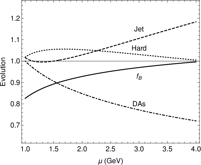
Figure 4: Evolution factors of the hard function, the BB-meson decay constant, the jet function and the BB-meson LCDA, which are denoted using dotted, solid, dashed and dot-dashed lines, respectively.
Refer to caption
Figure 5: The factorization-scale dependence of fB​π+​(0)f^{+}_{B\pi}(0). Solid, dotted, dot-dashed and dashed lines stand for values of the form factor with full RG evolution at NLL level, at LL level, with RG evolution only respect to the hard coefficient and the BB-meson decay constant and without RG evolution, respectively.

Before presenting numerical results of the form factors, we first show behaviors of evolution factors of the hard function (U1​(μ,μh​1)U_{1}(\mu,\mu_{h1})), the jet function (Uj​(μ,μh​c)U_{j}(\mu,\mu_{hc})), the BB-meson LCDA (U​ρ​(μ,μ0)U\rho(\mu,\mu_{0})) and the BB-meson decay constant (U2​(μ,μh​2)U_{2}(\mu,\mu_{h2})), in Fig.4. ω′\omega^{\prime} is fixed at 1.01.0GeV when plotting this figure. This choice leads to large logarithmic terms in evolution kernels of the LCDA and the jet function, hence evolution effects of these two functions are significant. But there is a strong cancellation between these two effects due to different signs of slopes of their curves. This cancellation is important to guarantee the scale invariance of the form factors. To illustrate the effect of the RG evolution, we plot in Fig.5 the scale dependence of fB​π(+)​(0)f^{(+)}_{B\pi}(0), where the first type of BB-meson LCDAs ϕB​1±​(ω)\phi^{\pm}_{B1}(\omega) and ρB​1−​(ω′)\rho^{-}_{B1}(\omega^{\prime}) are employed. It is obvious that after the complete RG evolution, the theoretical prediction of the form factor is almost independent of the factorization scale as expected. Results of fB​π(+)​(0)f^{(+)}_{B\pi}(0) with leading logarithm (LL) resummation and next-to-leading logarithm (NLL) resummation are both displayed for a comparison. It can be seen that the scale dependence is mild in both cases, but the NLL resummation reduces the value of the form factor about 3%3\% compared to the LL-resummation value. For terms contain ϕB+\phi_{B}^{+}, the RG evolution has not been performed (suppressed by the coupling constant). This figure also indicates that ϕB+\phi_{B}^{+} terms of the form factors are almost factorization-scale independent. In the numerical analysis, we set the factorization scale to be a hard-collinear scale (μ=1.5±0.5​GeV\mu=1.5\pm 0.5{\rm GeV}), as there are no large logarithmic terms in ϕB+\phi^{+}_{B} terms at this scale [16].

Refer to caption
Figure 6: The LCDA-model dependence of the vector form factor. Black, blue and red lines stand for the form factor computed with ρB​1−​(ω′,μ)\rho^{-}_{B1}{(\omega^{\prime},\mu)}, ρB​2−​(ω′,μ)\rho^{-}_{B2}{(\omega^{\prime},\mu)} and ρB​3−​(ω′,μ)\rho^{-}_{B3}{(\omega^{\prime},\mu)}, respectively.

Since BB-meson LCDAs are most important inputs of the BB-meson LCSR, we need to test the LCDA-model dependence of the form factors. In Fig.6, the vector form factor computed with three different B-meson LCDA models is displayed. Central values of the inverse moment are fitted as 0.392 in ρB​2−\rho^{-}_{B2} and 0.382 in ρB​3−\rho^{-}_{B3}. From this figure, we can see that model of the BB-meson LCDA has a tiny influence on the shape of the form factor. Hereafter we will take ρB​1−\rho^{-}_{B1} as the default model.

Refer to caption
Refer to caption
Figure 7: The Borel parameter and the effective threshold dependence of fB​π+​(0)f^{+}_{B\pi}(0). Solid, dot-dashed and dotted lines in the left (right) figure correspond to s0=0.7​GeV2s_{0}=0.7{\rm GeV^{2}}, 0.75​GeV20.75{\rm GeV^{2}} and 0.65​GeV20.65{\rm GeV^{2}} ( M2=1.25​GeV2M^{2}=1.25{\rm GeV^{2}}, 1.0​GeV21.0{\rm GeV^{2}} and 1.5​GeV21.5{\rm GeV^{2}}), respectively.

In the LCSR approach, the form factors should be insensitive to the Borel parameter and the effective threshold. These parameters are constrained following conditions in [16], where the contribution from excited and continuum states should be less than 40%40\% and the rate of change ∂ln⁡fB​πT​(q2)∂ln⁡ωM≤35%{\partial\ln f^{T}_{B\pi}(q^{2})\over\partial\ln\omega_{M}}\leq 35\%. We fix q2=0q^{2}=0 to study ωM\omega_{M} and s0s_{0} dependence of the form factors. Above constraints lead to a region 0.24≤ωM≤0.360.24\leq\omega_{M}\leq 0.36 (corresponding to 1.0≤M2/GeV2≤1.51.0\leq M^{2}/{\rm GeV^{2}}\leq 1.5) for all of the three form factors. We plot the Borel mass dependence of the form factor fB​π+​(0)f^{+}_{B\pi}(0) in Fig.(7), a manifest platform at M2∈[1.0​GeV2,1.5​GeV2]M^{2}\in[1.0{\rm GeV}^{2},1.5{\rm GeV}^{2}] guarantees that our calculation is insensitive to this unphysical parameter. The form factors are also almost independent on the effective threshold s0s_{0} when it is adopted as s0=(0.7±0.05)​GeV2s_{0}=(0.7\pm 0.05){\rm GeV^{2}}.

It has been argued that the B→πB\to\pi form factors calculated using the BB-meson LCSR can be trusted at q2≤qm​a​x2=8​GeV2q^{2}\leq q_{max}^{2}=8\,{\rm GeV^{2}} (see [11] for more detailed discussions). To extrapolate the form factors calculated with the BB-meson LCSR at large recoil toward large momentum transfer, we follow the same vein with [16], where the zz-series parameterization was employed. In this parameterization, the cut q2q^{2}-plane (the branch cut is the q2>t+q^{2}>t_{+} region of the real axis) is mapped onto the unit disk |z⁡(q2,t0)|<1|z(q^{2},t_{0})|<1 via the conformal transformation

z⁡(q2,t0)=t+−q2−t+−t0t+−q2+t+−t0,\displaystyle z(q^{2},t_{0})=\frac{\sqrt{t_{+}-q^{2}}-\sqrt{t_{+}-t_{0}}}{\sqrt{t_{+}-q^{2}}+\sqrt{t_{+}-t_{0}}}\,, (50)

where t+=(mB+mπ)2t_{+}=(m_{B}+m_{\pi})^{2} denotes the threshold of continuum states in the B∗B^{\ast}-meson channel. The free parameter t0∈(−∞,t+)t_{0}\in(-\infty\,,t_{+}) determines the value of q2q^{2} mapped onto the origin in the zz plane. One can adjust the value of t0t_{0} to minimize the corresponding zz interval in the region qm​i​n2≤q2≤qm​a​x2q_{min}^{2}\leq q^{2}\leq q_{max}^{2}, in order that the zz-series expansion converges rapidly. Here we choose the same value as that in [8]

t0=t+2−t+−t−​t+−qm​i​n2,\displaystyle t_{0}=t_{+}^{2}-\sqrt{t_{+}-t_{-}}\,\sqrt{t_{+}-q_{min}^{2}}\,, (51)

where qm​i​n2=−6.0​GeV2q_{min}^{2}=-6.0\,{\rm GeV^{2}} and t−≡(mB−mπ)2t_{-}\equiv(m_{B}-m_{\pi})^{2}. Using the zz-series expansion and taking into account the threshold t+t_{+} behavior, one can obtain the parametrization of each form factor.

Parametrizations of the vector and the scalar form factors have been given in [32, 8]. The parametrization of the tensor form factor is similar with that of fB​π+​(q2)f^{+}_{B\pi}(q^{2}) [33]

fB​πT(q2)=fB​πT​(0)1−q2/mB∗2{1+∑k=1N−1bkT(z(q2,t0)k−z(0,t0)k\displaystyle f^{T}_{B\pi}(q^{2})=\frac{f^{T}_{B\pi}(0)}{1-q^{2}/m_{B^{*}}^{2}}\Bigg\{1+\sum\limits_{k=1}^{N-1}b^{T}_{k}\,\Bigg(z(q^{2},t_{0})^{k}-z(0,t_{0})^{k}
−(−1)N−kkN[z(q2,t0)N−z(0,t0)N])},\displaystyle-(-1)^{N-k}\frac{k}{N}\bigg[z(q^{2},t_{0})^{N}-z(0,t_{0})^{N}\bigg]\Bigg)\Bigg\}\,, (52)

where the expansion coefficient(s) bkTb^{T}_{k} is (are) determined by matching the large-recoil fB​πT​(q2)f^{T}_{B\pi}(q^{2}) onto Eq.(52). As the interval in the zz plane is constrained in a small region, it is reasonable to truncate the zz-series at N=2N=2 in the practical calculation. Slop parameters b1,b~1,b1Tb_{1},\,\tilde{b}_{1},\,b_{1}^{T} are collected in Table 1. Uncertainties from different sources, including the inverse moment, the model of BB-meson LCDA, the Borel parameter, the effective threshold, quark masses, et al, are taken into account in our numerical analysis. In Table 1, we collect parameters which arise large uncertainties.

Parameter default λB​(1​GeV)\lambda_{B}(1\text{GeV}) ωM\omega_{M} mb¯​(mb¯)\overline{m_{b}}(\overline{m_{b}}) s0Bs^{B}_{0} LCDA
fB​π+​(0)f^{+}_{B\pi}(0) 0.2540.254 −0.024+0.022{}^{+0.022}_{-0.024} −0.012+0.008{}^{+0.008}_{-0.012} −0.011+0.009{}^{+0.009}_{-0.011} −0.006+0.011{}^{+0.011}_{-0.006} −0.000+0.075{}^{+0.075}_{-0.000}
fB​πT​(0)f^{T}_{B\pi}(0) 0.2540.254 −0.024+0.022{}^{+0.022}_{-0.024} −0.012+0.007{}^{+0.007}_{-0.012} −0.012+0.009{}^{+0.009}_{-0.012} −0.006+0.011{}^{+0.011}_{-0.006} −0.000+0.076{}^{+0.076}_{-0.000}
b1b_{1} −4.13-4.13 −0.09+0.08{}^{+0.08}_{-0.09} −0.05+0.02{}^{+0.02}_{-0.05} −0.01+0.00{}^{+0.00}_{-0.01} −0.01+0.00{}^{+0.00}_{-0.01} −0.00+0.64{}^{+0.64}_{-0.00}
b~1\tilde{b}_{1} −5.56-5.56 −0.12+0.11{}^{+0.11}_{-0.12} −0.06+0.03{}^{+0.03}_{-0.06} −0.01+0.00{}^{+0.00}_{-0.01} −0.00+0.00{}^{+0.00}_{-0.00} −0.00+0.79{}^{+0.79}_{-0.00}
b1Tb^{T}_{1} −4.42-4.42 −0.11+0.08{}^{+0.08}_{-0.11} −0.10+0.02{}^{+0.02}_{-0.10} −0.01+0.00{}^{+0.00}_{-0.01} −0.01+0.00{}^{+0.00}_{-0.01} −0.00+0.71{}^{+0.71}_{-0.00}
Table 1: zz-parameter fitted values of fB​π+​(0)f^{+}_{B\pi}(0), fB​πT​(0)f^{T}_{B\pi}(0), b1b_{1}, b~1\tilde{b}_{1} and b1Tb^{T}_{1} (fB​π0​(0)f^{0}_{B\pi}(0) is not listed here because fB​π0​(0)=fB​π+​(0)f^{0}_{B\pi}(0)=f^{+}_{B\pi}(0)). The notation “default” means that all of the parameters are taken as central values.
Refer to caption
Refer to caption
Figure 8: q2q^{2} dependence of the form factor fB​π0​(q2)f^{0}_{B\pi}(q^{2}), and the re-scaled form factor fB​π+​(q2)f^{+}_{B\pi}(q^{2}). Black and red curves are results of the BB-meson and the pion LCSRs, respectively. Lattice QCD results are taken from HPQCD collaboration [34] (blue squres), Fermilab/MILC collaboration [35] (blue band) and RBC/UKQCD collaboration [36] (green and blue triangles).

In Fig.(8) the q2q^{2} dependence of form factors fB​π0,+​(q2)f^{0,+}_{B\pi}(q^{2}) are shown, where Lattice results are from HPQCD collaboration [34], Fermilab/MILC collaboration [35] and RBC/UKQCD collaboration [36]. Our results of fB​π0f^{0}_{B\pi} within errors are in agreement with the Lattice data. While our results of fB​π+f^{+}_{B\pi} is larger than the Lattice data. Results of fB​π0,+​(q2)f^{0,+}_{B\pi}(q^{2}) from the pion LCSR are also shown. It is manifest that slopes of these two form factors with the BB-meson LCSR are greater than that of the pion LCSR. The difference between the BB-meson and other approaches can be understood through following points. (1) As we can see from Table 1, the parameter λB\lambda_{B} brings huge uncertainty to results of the form factors. Values of the form factors at q2=0​GeV2q^{2}=0\,{\rm GeV^{2}} are significantly influenced by the changing of λB\lambda_{B}. But the value of this parameter is not determined yet. (2) We only calculate leading-power contributions of the form factors in this work. While power-suppressed contributions, which are induced by higher-twist pion LCDAs, are taken into account in calculations of the pion LCSR. The subleading-power effect in the BB-meson LCSR may influence both values of the form factors at q2=0​GeV2q^{2}=0\,{\rm GeV^{2}} and slopes of the form factors.

Refer to caption
Figure 9: The normalized differential q2q^{2} distribution of B→π​μ​νμB\to\pi\mu\nu_{\mu}. The black solid curve represents the central value of our prediction and black dashed curves correspond to uncertainties. Experimental data bins are from [38] (blue stars), [39] (red stars), [40] (blue circles), [41] (blue triangles) and [42] (red circles).

B→πB\to\pi form factors are very important phenomenologically. Here we briefly discuss two applications of our result. The CKM matrix element |Vu​b||V_{ub}| can be determined from the (partial) branching fraction of B→π​ℓ​νℓB\to\pi\ell\nu_{\ell}. If we neglect mass of leptons, the integrated decay width is written by

∫0q02d​q2​d​Γd​q2​(B→π​l​ν)\displaystyle\int_{0}^{q_{0}^{2}}dq^{2}\frac{d\Gamma}{dq^{2}}\,(B\to\pi l\nu) ≡|Vu​b|2​Δ​ζ​(0,q02),\displaystyle\equiv|V_{ub}|^{2}\Delta\zeta(0,q_{0}^{2})\,, (53)

where |p→π||\vec{p}_{\pi}| is the magnitude of the pion three-momentum in the BB-meson rest frame, l=e,μl=e,\mu and

Δ​ζ​(0,q02)=GF224​π3​∫0q02d​q2​|p→π|3​|fB​π+​(q2)|2.\displaystyle\Delta\zeta(0,q_{0}^{2})=\frac{G_{F}^{2}}{24\pi^{3}}\,\int_{0}^{q_{0}^{2}}\,dq^{2}\,|\vec{p}_{\pi}|^{3}\,\,|f_{B\pi}^{+}(q^{2})|^{2}\,. (54)

A straightforward extraction of |Vu​b||V_{ub}| can be performed using the relation

|Vu​b|2=Δ​ℬℛ​(0,q02)​τB0Δ​ζ​(0,q02),\displaystyle|V_{ub}|^{2}={\Delta{\cal BR}(0,q_{0}^{2})\tau_{B^{0}}\over\,\Delta\zeta(0,q_{0}^{2})\,}, (55)

where Δ​ℬℛ​(0,q02)\Delta{\cal BR}(0,q_{0}^{2}) is the integrated branching ratio and the mean lifetime of the B0B^{0} meson τB0=(1.519±0.005)​ps\tau_{B^{0}}=(1.519\pm 0.005)\,{\rm ps} [37]. Experimental measurements of Δ​ℬℛ​(0,q02)\Delta{\cal BR}(0,q_{0}^{2}) of the semi-leptonic B¯0→π+​μ​νμ\bar{B}^{0}\to\pi^{+}\,\mu\,\nu_{\mu} decay [38, 39] are given by

Δ​ℬℛ​(0,12​GeV2)\displaystyle\Delta{\cal BR}(0,12\,{\rm GeV^{2}}) =\displaystyle= (0.83±0.03±0.04)×10−4,[BaBar​  2012]\displaystyle(0.83\pm 0.03\pm 0.04)\times 10^{-4}\,,\hskip 25.6073pt{\rm[BaBar\,\,2012]}
Δ​ℬℛ​(0,12​GeV2)\displaystyle\Delta{\cal BR}(0,12\,{\rm GeV^{2}}) =\displaystyle= (0.808±0.062)×10−4.[Belle​      2013]\displaystyle(0.808\pm 0.062)\times 10^{-4}\,.\hskip 48.36958pt{\rm[Belle\,\,\,\,\,\,2013]} (56)

Utilizing the result of the form factor fB​π+​(q2)f_{B\pi}^{+}(q^{2}) which is computed with the BB-meson LCSR and extrapolated with the zz-series parametrization we can obtain

Δ​ζ​(0,12​GeV2)\displaystyle\Delta\zeta(0,12\,{\rm GeV^{2}}) =\displaystyle= 4.93+0.30−0.05|ω0+0.36−0.41|ωM+0.44−0.23|s0+2.79−0|ϕBps−1\displaystyle 4.93\,\,{}^{+0.30}_{-0.05}\Big|_{\omega_{0}}\,\,{}^{+0.36}_{-0.41}\Big|_{\omega_{M}}\,\,{}^{+0.44}_{-0.23}\Big|_{s_{0}}\,\,{}^{+2.79}_{-0}\Big|_{\phi_{B}}\,\,\mbox{ps}^{-1} (57)
=\displaystyle= 4.93−0.97+2.99​ps−1.\displaystyle 4.93^{+2.99}_{-0.97}~\mbox{ps}^{-1}\,.

Then the extracted CKM matrix element

|Vu​b|=(3.33−0.74+0.37|th.±0.09|exp.)×10−3,\displaystyle|V_{ub}|=\left(3.33^{+0.37}_{-0.74}|_{\rm th.}\pm 0.09|_{\rm exp.}\right)\times 10^{-3}\,, (58)

where the theoretical uncertainty comes from uncertainties of Δ​ζ​(0,12​GeV2)\Delta\zeta(0,12\,{\rm GeV^{2}}) as displayed in (57). This |Vu​b||V_{ub}| is larger compared to [16], since the RG evolution reduces the value of fB​π+​(q2)f_{B\pi}^{+}(q^{2}). In Fig.9, we display the normalized differential q2q^{2} distribution of B→π​μ​νμB\to\pi\mu\nu_{\mu}. Black curves represent the prediction of this work, where the solid line is the central value and dashed curves correspond to uncertainties. Due to the cancellation of the uncertainty of fB​π+​(q2)f_{B\pi}^{+}(q^{2}), the uncertainty of the normalized differential distribution of B→π​μ​νμB\to\pi\mu\nu_{\mu} is small. Our prediction is in agreement with the experimental data from BarBar [38, 40, 41] and Belle [39, 42].

5 CONCLUSION AND DISCUSSION

We reviewed the method of calculating the B→πB\to\pi tensor form factor with the BB-meson LCSR. In this framework, the method of regions was employed and contributions from different momentum regions are separated naturally. Precise soft cancellation guarantees the factorization theorem. The correlation function was factorized into the convolution of the hard function, the jet function and the BB-meson LCDA which correspond to contributions from hard, hard-collinear and soft regions, respectively. We obtained one-loop-level hard and jet functions through the analysis of symmetry-breaking effects.

To resum large logarithmic terms in the form factors, we carried out the complete RG evolution of the factorized correlation function, including evolutions of the jet function and the BB-meson LCDA. The BB-meson LCDA, defined via the HQET, obey the Lange-Neubert equation which contains non-diagonal anomalous dimension. Following the approach in [24], we diagonalized the RG equation of the BB-meson LCDA in the dual space and solved the diagonalized RG equation. The same method was also applied to the evolution of the jet function. Combining the evolution of each part together, we obtained the RG improved B→πB\to\pi form factors.

On the numerical side, we checked behaviors of the four evolution kernels (U1,U2,Uj​and​UρU_{1},\,U_{2},\,U_{j}\,{\rm and}\,U_{\rho}) and illustrated cancellation effects among the kernels. We examined the factorization-scale dependence of the RG improved form factors and compared our predictions with previous results. We extrapolated the q2q^{2} dependence of the form factors to the whole physical region using the zz-series expansion. Then we compared values of the form factors in this work with that in the LQCD and the pion LCSR. Phenomenologically we extracted the CKM matrix element |Vu​b||V_{ub}| and analysed the normalized differential q2q^{2} dependence of B→π​μ​νμB\to\pi\mu\nu_{\mu}. The BB-meson form factors have many other phenomenological applications, such as the tensor form factor can give important contributions to FCNC processes B→(π,K)​l+​l−B\to(\pi,K)l^{+}l^{-}. Of course a complete study of phenomenological applications are far more complicated, and we left it for the future work. This work supplements the framework proposed in [16], and can be applied to various transition processes.

Acknowledgement

We are grateful to Y. M. Wang for useful discussions and comments. This work was supported in part by Natural Science Foundation of Shandong Province, China under Grant No. ZR2015AQ006 and by National Natural Science Foundation of China (Grants No. 11375208, No. 11521505, No. 11235005, No. 11447009).

Appendix A Jet function in the dual space

The jet function in the dual space is defined by

j(−)​(μh​c2n⋅p​ω^′,ω^′n¯⋅p)\displaystyle j^{(-)}\left({\mu_{hc}^{2}\over n\cdot p\hat{\omega}^{\prime}},{\hat{\omega}^{\prime}\over\bar{n}\cdot p}\right) =\displaystyle= ∫0∞d​ωω−n¯⋅p​J0​(2​ωω′)​J(−)​(μ2n⋅p​ω,ωn¯⋅p)\displaystyle\int^{\infty}_{0}\frac{d\omega}{\omega-\bar{n}\cdot p}J_{0}(2\sqrt{\frac{\omega}{\omega^{\prime}}}){J}^{(-)}\left({\mu^{2}\over n\cdot p\,\omega},{\omega\over\bar{n}\cdot p}\right) (59)
=\displaystyle= ∫0∞d​η1+η​J0​(2​ηη′)​J(−)​(η,μ),\displaystyle\int^{\infty}_{0}\frac{d\eta}{1+\eta}J_{0}(2\sqrt{\frac{\eta}{\eta^{\prime}}}){J}^{(-)}(\eta,\mu),

where

J(−)​(η,μ)\displaystyle J^{(-)}(\eta,\mu) =\displaystyle= 1+αs​CF4​π[ln2μ2−p2−2ln(1+η)lnμ2−p2\displaystyle 1+\frac{\alpha_{s}\,C_{F}}{4\,\pi}\,\bigg[\ln^{2}{\mu^{2}\over-p^{2}}-2\ln{(1+\eta)}\ln{\mu^{2}\over-p^{2}} (60)
+\displaystyle+ ln2(1+η)−η−2ηln(1+η)−π26−1].\displaystyle\ln^{2}(1+\eta)-\frac{\eta-2}{\eta}\ln{(1+\eta)}-{\pi^{2}\over 6}-1\bigg]\,.

Using the formula

∫0∞x​d​x(x2+k2)1−λ​J0​(a​x)=1Γ⁡(1−λ)​(2​ka)λ​Kλ​(k​a),\displaystyle\int^{\infty}_{0}\frac{xdx}{(x^{2}+k^{2})^{1-\lambda}}J_{0}(ax)=\frac{1}{\Gamma(1-\lambda)}(\frac{2k}{a})^{\lambda}K_{\lambda}(ka), (61)

which is valid for λ<3/4\lambda<3/4, and performing derivative with respect to λ\lambda, and taking the limit λ→0\lambda\to 0, we can get

∫0∞d​η1+η​J0​(2​ηη′)\displaystyle\int^{\infty}_{0}\frac{d\eta}{1+\eta}J_{0}\left(2\sqrt{\frac{\eta}{\eta^{\prime}}}\right) =\displaystyle= 2​K0​(2​1η′),\displaystyle 2K_{0}\left(2\sqrt{\frac{1}{\eta^{\prime}}}\right),
∫0∞d​η1+η​J0​(2​ηη′)​ln⁡(1+η)\displaystyle\int^{\infty}_{0}\frac{d\eta}{1+\eta}J_{0}\left(2\sqrt{\frac{\eta}{\eta^{\prime}}}\right)\ln(1+\eta) =\displaystyle= (ln⁡η′−2​γE)​K0​(2​1η′),\displaystyle(\ln\eta^{\prime}-2\gamma_{E})K_{0}\left(2\sqrt{\frac{1}{\eta^{\prime}}}\right),
∫0∞d​η1+η​J0​(2​ηη′)​ln2⁡(1+η)\displaystyle\int^{\infty}_{0}\frac{d\eta}{1+\eta}J_{0}\left(2\sqrt{\frac{\eta}{\eta^{\prime}}}\right)\ln^{2}(1+\eta) =\displaystyle= [12​ln2​η′−2​γE​ln⁡η′+2​γE2−2​ψ′​(1)]​K0​(2​1η′)\displaystyle[\frac{1}{2}\ln^{2}\eta^{\prime}-2\gamma_{E}\ln\eta^{\prime}+2\gamma_{E}^{2}-2\psi^{\prime}(1)]K_{0}\left(2\sqrt{\frac{1}{\eta^{\prime}}}\right) (62)
+\displaystyle+ 2​K0(2,0)​(2​1η′).\displaystyle 2K^{(2,0)}_{0}\left(2\sqrt{\frac{1}{\eta^{\prime}}}\right).

Another useful equation is

∫0∞d​xx​J0​(b​x)​ln⁡(1+x2)​𝑑x=2​∫b∞K0​(β)β​𝑑β.\displaystyle\int^{\infty}_{0}\frac{dx}{x}J_{0}(bx)\ln(1+x^{2})dx=2\int_{b}^{\infty}\frac{K_{0}(\beta)}{\beta}d\beta. (63)

Taking the advantage of Eqs. (62) and (63), one can obtain Eq. (40).

Appendix B Dispersion integrals

To obtain final expressions of the form factors, we need to extrapolate n¯⋅p\bar{n}\cdot p to physical region. For the consistency of our derivation, we must have

∫0∞d​ωω−Ω−i​ϵ​J0​(2​ωω′)\displaystyle\int^{\infty}_{0}\frac{d\omega}{\omega-\Omega-i\epsilon}J_{0}\left(2\sqrt{\frac{\omega}{\omega^{\prime}}}\right) =\displaystyle= 2​K0​(−2​i​Ωω′).\displaystyle 2K_{0}\left(-2i\sqrt{\frac{\Omega}{\omega^{\prime}}}\right).

The above equation indicates that the branch cut of the root and logarithmic function be along negative real axis, and −Ω−i​ϵ=Ω​e−i​π-\Omega-i\epsilon=\Omega e^{-i\pi}. The following equation can be derived from Eq. (61)

∫0∞d​ωω−Ω−i​ϵ​(1−ωΩ)λ​J0​(2​ωω′)\displaystyle\int^{\infty}_{0}\frac{d\omega}{\omega-\Omega-i\epsilon}(1-{\omega\over\Omega})^{\lambda}J_{0}\left(2\sqrt{\frac{\omega}{\omega^{\prime}}}\right) =\displaystyle= i​π​ei​λ​π​(ω′Ω)λ/2​1Γ⁡(1−λ)​Hλ(1)​(2​Ωω′).\displaystyle i\pi e^{i\lambda\pi}\left({\omega^{\prime}\over\Omega}\right)^{\lambda/2}\frac{1}{\Gamma(1-\lambda)}H_{\lambda}^{(1)}\left(2\sqrt{\frac{\Omega}{\omega^{\prime}}}\right). (65)

From which we obtain following useful results:

∫0∞d​ωω−Ω−i​ϵ​ln⁡(1−ωΩ)​J0​(2​ωω′)\displaystyle\int^{\infty}_{0}\frac{d\omega}{\omega-\Omega-i\epsilon}\ln(1-{\omega\over\Omega})J_{0}\left(2\sqrt{\frac{\omega}{\omega^{\prime}}}\right) =\displaystyle= −π22​J0​(2​Ωω′)−π2​ln⁡ω^′Ω​N0​(2​Ωω′)\displaystyle-{\pi^{2}\over 2}J_{0}\left(2\sqrt{\frac{\Omega}{\omega^{\prime}}}\right)-{\pi\over 2}\ln{\hat{\omega}^{\prime}\over\Omega}N_{0}\left(2\sqrt{\frac{\Omega}{\omega^{\prime}}}\right) (66)
−\displaystyle- i⁡[π22​N0​(2​Ωω′)−π2​ln⁡ω^′Ω​J0​(2​Ωω′)],\displaystyle i\left[{\pi^{2}\over 2}N_{0}\left(2\sqrt{\frac{\Omega}{\omega^{\prime}}}\right)-{\pi\over 2}\ln{\hat{\omega}^{\prime}\over\Omega}J_{0}\left(2\sqrt{\frac{\Omega}{\omega^{\prime}}}\right)\right],
∫0∞d​ωω−Ω−i​ϵ​ln2⁡(1−ωΩ)​J0​(2​ωω′)\displaystyle\int^{\infty}_{0}\frac{d\omega}{\omega-\Omega-i\epsilon}\ln^{2}(1-{\omega\over\Omega})J_{0}\left(2\sqrt{\frac{\omega}{\omega^{\prime}}}\right) =\displaystyle= i​π2​(12​ln2​ω^′Ω+i​π​ln⁡ω^′Ω−π23)​H0(1)​(2​Ωω′)\displaystyle{i\pi\over 2}\left({1\over 2}\ln^{2}{\hat{\omega}^{\prime}\over\Omega}+i\pi\ln{\hat{\omega}^{\prime}\over\Omega}-{\pi^{2}\over 3}\right)H^{(1)}_{0}\left(2\sqrt{\frac{\Omega}{\omega^{\prime}}}\right) (67)
+\displaystyle+ i​π​J0(2,0)​(2​Ωω′)−π​N0(2,0)​(2​Ωω′).\displaystyle i\pi J^{(2,0)}_{0}\left(2\sqrt{\frac{\Omega}{\omega^{\prime}}}\right)-\pi N^{(2,0)}_{0}\left(2\sqrt{\frac{\Omega}{\omega^{\prime}}}\right).

Following a similar way, another useful result is also obtained

∫0∞d​ωω​ln⁡(1−ωΩ)​J0​(2​ωω′)\displaystyle\int^{\infty}_{0}\frac{d\omega}{\omega}\ln(1-{\omega\over\Omega})J_{0}\left(2\sqrt{\frac{\omega}{\omega^{\prime}}}\right) =\displaystyle= 2​i​π​∫2​Ωω′∞d​ββ​H0(1)​(β).\displaystyle 2i\pi\int^{\infty}_{2\sqrt{\frac{\Omega}{\omega^{\prime}}}}\frac{d\beta}{\beta}H^{(1)}_{0}(\beta). (68)

Taking the imaginary part of the above equation, we have

Im​∫0∞d​ωω​ln⁡(1−ωΩ)​J0​(2​ωω′)=2​π​[−γE+Ωω′​F32​(1,1,2,2,2,−Ωω′)−ln⁡Ωω^′].{\rm Im}\int^{\infty}_{0}\frac{d\omega}{\omega}\ln(1-{\omega\over\Omega})J_{0}\left(2\sqrt{\frac{\omega}{\omega^{\prime}}}\right)=2\pi\left[-\gamma_{E}+\frac{\Omega}{\omega^{\prime}}{{}_{2}F_{3}}(1,1;2,2,2;-\frac{\Omega}{\omega^{\prime}})-\ln\frac{\Omega}{\hat{\omega}^{\prime}}\right]. (69)

Having all of above equations in hand, we get final results in Eqs. (43) and (44).

References

  • [1] V. M. Belyaev, A. Khodjamirian and R. Ruckl, Z. Phys. C 60, 349 (1993) [hep-ph/9305348].
  • [2] A. Khodjamirian, R. Ruckl, S. Weinzierl and O. I. Yakovlev, Phys. Lett. B 410, 275 (1997) [hep-ph/9706303].
  • [3] E. Bagan, P. Ball and V. M. Braun, Phys. Lett. B 417, 154 (1998) [hep-ph/9709243].
  • [4] P. Ball and R. Zwicky, JHEP 0110 (2001) 019 [hep-ph/0110115].
  • [5] P. Ball and R. Zwicky, Phys. Rev. D 71 (2005) 014015 [hep-ph/0406232].
  • [6] G. Duplancic, A. Khodjamirian, T. Mannel, B. Melic and N. Offen, JHEP 0804 (2008) 014 [arXiv:0801.1796 [hep-ph]].
  • [7] A. Bharucha, JHEP 1205 (2012) 092 [arXiv:1203.1359 [hep-ph]].
  • [8] A. Khodjamirian, T. Mannel, N. Offen and Y.-M. Wang, Phys. Rev. D 83 (2011) 094031 [arXiv:1103.2655 [hep-ph]].
  • [9] E. P. Kadantseva, S. V. Mikhailov and A. V. Radyushkin, Yad. Fiz. 44, 507 (1986) [Sov. J. Nucl. Phys. 44, 326 (1986)].
  • [10] A. Khodjamirian, T. Mannel and N. Offen, Phys. Lett. B 620 (2005) 52 [hep-ph/0504091].
  • [11] A. Khodjamirian, T. Mannel and N. Offen, Phys. Rev. D 75 (2007) 054013 [hep-ph/0611193].
  • [12] C. W. Bauer, S. Fleming, D. Pirjol and I. W. Stewart, Phys. Rev. D 63 (2001) 114020 [hep-ph/0011336].
  • [13] M. Beneke, A. P. Chapovsky, M. Diehl and T. Feldmann, Nucl. Phys. B 643, 431 (2002) [hep-ph/0206152].
  • [14] F. De Fazio, T. Feldmann and T. Hurth, Nucl. Phys. B 733 (2006) 1 [Nucl. Phys. B 800 (2008) 405] [hep-ph/0504088].
  • [15] F. De Fazio, T. Feldmann and T. Hurth, JHEP 0802 (2008) 031 [arXiv:0711.3999 [hep-ph]].
  • [16] Y. Wang and Y. Shen, Nucl. Phys. B 898 (2015) 563 [arXiv:1506.00667 [hep-ph]].
  • [17] M. Beneke and V. A. Smirnov, Nucl. Phys. B 522 (1998) 321 [hep-ph/9711391].
  • [18] M. Beneke and T. Feldmann, Nucl. Phys. B 592 (2001) 3 [hep-ph/0008255].
  • [19] G. Sterman, An Introduction to Quantum Field Theory (Cambridge University Press, Cambridge, 1993).
  • [20] M. Beneke, Y. Kiyo and D. S. Yang, Nucl. Phys. B 692 (2004) 232 [hep-ph/0402241].
  • [21] M. Beneke and D. S. Yang, Nucl. Phys. B 736 (2006) 34 [hep-ph/0508250].
  • [22] A. G. Grozin and M. Neubert, Phys. Rev. D 55 (1997) 272 [hep-ph/9607366].
  • [23] B. O. Lange and M. Neubert, Phys. Rev. Lett. 91 (2003) 102001 [hep-ph/0303082].
  • [24] G. Bell, T. Feldmann, Y. M. Wang and M. W. Y. Yip, JHEP 1311 (2013) 191 [arXiv:1308.6114 [hep-ph]].
  • [25] M. Beneke and T. Feldmann, Nucl. Phys. B 685 (2004) 249 [hep-ph/0311335].
  • [26] S. Descotes-Genon and C. T. Sachrajda, Nucl. Phys. B 650 (2003) 356 [hep-ph/0209216].
  • [27] M. Beneke and J. Rohrwild, Eur. Phys. J. C 71 (2011) 1818 [arXiv:1110.3228 [hep-ph]].
  • [28] V. M. Braun and A. N. Manashov, Phys. Lett. B 731 (2014) 316 [arXiv:1402.5822 [hep-ph]].
  • [29] V. M. Braun, D. Y. Ivanov and G. P. Korchemsky, Phys. Rev. D 69 (2004) 034014 [hep-ph/0309330].
  • [30] H. Kawamura, J. Kodaira, C. F. Qiao and K. Tanaka, Phys. Lett. B 523, 111 (2001) Erratum: [Phys. Lett. B 536, 344 (2002)] [hep-ph/0109181].
  • [31] T. Feldmann, B. O. Lange and Y. M. Wang, Phys. Rev. D 89 (2014) 11, 114001 [arXiv:1404.1343 [hep-ph]].
  • [32] C. Bourrely, I. Caprini and L. Lellouch, Phys. Rev. D 79 (2009) 013008 [Phys. Rev. D 82 (2010) 099902] [arXiv:0807.2722 [hep-ph]].
  • [33] Z. H. Li, Z. G. Si, Y. Wang and N. Zhu, Nucl. Phys. B 900, 198 (2015).
  • [34] J. M. Flynn, T. Izubuchi, T. Kawanai, C. Lehner, A. Soni, R. S. Van de Water and O. Witzel, Phys. Rev. D 91 (2015) 7, 074510 [arXiv:1501.05373 [hep-lat]].
  • [35] J. A. Bailey et al. [Fermilab Lattice and MILC Collaborations], Phys. Rev. D 92, no. 1, 014024 (2015) [arXiv:1503.07839 [hep-lat]].
  • [36] E. Dalgic, A. Gray, M. Wingate, C. T. H. Davies, G. P. Lepage and J. Shigemitsu, Phys. Rev. D 73 (2006) 074502 [Phys. Rev. D 75 (2007) 119906] [hep-lat/0601021].
  • [37] K. A. Olive et al. [Particle Data Group Collaboration], Chin. Phys. C 38 (2014) 090001.
  • [38] J. P. Lees et al. [BaBar Collaboration], Phys. Rev. D 86 (2012) 092004 [arXiv:1208.1253 [hep-ex]].
  • [39] A. Sibidanov et al. [Belle Collaboration], Phys. Rev. D 88 (2013) 3, 032005 [arXiv:1306.2781 [hep-ex]].
  • [40] P. del Amo Sanchez et al. [BaBar Collaboration], Phys. Rev. D 83, 032007 (2011) [arXiv:1005.3288 [hep-ex]].
  • [41] P. del Amo Sanchez et al. [BaBar Collaboration], Phys. Rev. D 83, 052011 (2011) [arXiv:1010.0987 [hep-ex]].
  • [42] H. Ha et al. [Belle Collaboration], Phys. Rev. D 83, 071101 (2011) [arXiv:1012.0090 [hep-ex]].