Relic Abundance in a Secluded Dark Matter Scenario with a Massive Mediator
Abstract
The relic abundance of the dark matter (DM) particle is studied in a secluded DM scenario, in which the number decreasing process dominantly occurs not through the pair annihilation of into the standard model particles, but via the scattering process with a subsequently decaying mediator particle . It is pointed out that the cosmologically observed relic abundance of DM can be accomplished even with a massive mediator having a mass non-negligibly heavy compared with the DM particle mass . In the degenerated - case (), the DM relic abundance is realized by adjusting the scattering amplitude large enough and by choosing an appropriate mediator particle life-time. The DM evolution in the early universe exhibits characteristic “terrace” behavior, or two-step number density decreasing behavior, having a “fake” freeze-out at the first step. Based on these observations, a novel possibility of the DM model buildings is introduced in which the mediator particle is unified with the DM particle in an approximate dark symmetry multiplet. A pionic DM model is proposed to illustrate this idea in a renormalizable field theory framework.
pacs
12.60.-i, 12.60.Rc, 95.35.+dI Introduction
More than 80% of the matter is made up of Dark Matter (DM) in the universe[1, 2, 3]. Very little of the DM nature is known, however, besides its cosmological abundance [3].
Theories beyond the standard model (BSM) in particle physics often predict the existence of new massive particles. The lightest neutral stable new particle, if it exists in these BSM scenarios, provides an excellent DM candidate, longevity of which is guaranteed by a new symmetry existing in the BSM scenario. For reviews, see, e.g., Refs.[4, 5].
A promising hypothesis we are able to make in these DM models is that the DM particles were produced thermally in the early universe (thermal relic hypothesis)[6] and the cosmological DM abundance can be computed through the Boltzmann equation, once the mass and the couplings of the DM particle are fixed. It has been widely assumed that the DM number density decreasing process was dominated by the pair annihilation of the DM particles into the standard model (SM) particles. If this is true, the DM particle mass and its couplings with the SM particles can be related with each other through the observed value of the cosmological DM abundance. Assuming further the DM pair annihilation cross section is determined by the couplings of the order of the electroweak gauge coupling strengths, the thermal relic hypothesis predicts the DM particle mass of the weak scale. This striking coincidence is often called the “WIMP Miracle”. The heavier DM particle mass, the stronger DM couplings with the SM sector we need to assume in this widely adopted thermal relic scenarios: we therefore cannot seclude the DM particles from the SM sector. This tendency has encouraged the DM particle searches in the direct detection experiments [7] and in the collider experiments [8]. It is unfortunate, however, up to the present time, we have no fully confidently positive results in these DM particle search experiments [7, 9, 10, 11, 12, 13].
Recently, new varieties of thermal relic DM scenarios have been proposed. In these scenarios, interactions between the DM particles and the SM particles are weak enough to make the scenarios consistent with the present and near future constraints from the direct DM detections and the collider experiments, still keeping the observed value of the cosmological DM abundance, by introducing novel mechanisms to decrease the DM particle number density in the thermal history of the early universe.
The authors of Refs.[14, 15] consider a scenario in which the relic density is controlled by the scattering process among the DM particles, instead of the traditional process of the DM pair annihilation into the SM particles. The cross section for the scattering enough to explain the observed DM abundance may be achieved in the DM model associated with dark strong dynamics, assuming the dark pions to be the DM particle. The anomaly induced Wess-Zumino-Witten (WZW) term[16, 17] in the dark chiral Lagrangian naturally explains the required scattering in the dark sector. Although the dark sector in this scenario is chemically secluded from the visible sector, it is assumed to interact with the SM sector very weakly, keeping the dark sector temperature equal to the visible sector in the epoch of the DM particle number decreasing processes. It has been pointed out, however, the WZW induced scattering annihilation process may not be enough to reduce the DM number density if the higher order effects are incorporated consistently in the chiral perturbation framework.
Refs.[18, 19] introduce a phenomenological scenario in which the DM number density decreasing mechanism is implemented by the DM pair annihilation into additional non-SM particles (mediator particles) through the process (the secluded DM scenario). The mediator is assumed to decay into the SM particles later and is sufficiently lighter than the DM particle. Note here the mass hierarchy between the two separate mass scales (the DM mass and the mediator mass ), , is introduced on an ad hoc basis in this scenario. With a large mass gap , the DM relic abundance is insensitive to the mediator particle life-time. It is assumed that the dark sector decouples chemically from the visible sector in the early epoch of its thermal history, but it follows the visible sector temperature, keeping the kinematical equilibrium with the SM particles.
The authors of Ref.[20] propose a DM sector almost completely decoupled from the SM sector both kinematically and chemically (cannibal DM). Novel mechanisms similar to SIMP and the secluded DM are responsible for the DM particle number decreasing process in the dark sector. Since the dark sector is decoupled from the SM sector almost completely, the DM particle temperature differs from the SM sector in the thermal history of the universe. Ref.[21] considers a similar scenario having the dark sector kinematically decoupled from the visible sector. The late time decay of new particles into the SM sector, which were produced copiously in the dark sector thermal history, reheats the visible sector and dilutes the DM density.
In this paper, we solve the Boltzmann equation numerically in a toy secluded DM model having a heavy mediator . The secluded DM having a large mass gap , as well as the familiar mechanism of the DM pair annihilation into the SM particles, can also be analyzed in this toy model. We point out the seclusion mechanism works well even with if the mediator life-time is short enough, in contrast to the original secluded DM proposal having a large mass gap and a longer life-time mediator. The hierarchy assumption made ad hoc in Refs.[18, 19] is, therefore, not necessary. We notice that the departure of the mediator number density from its thermoequilibrium value causes non-negligible effects in the evaluation of the DM relic density.
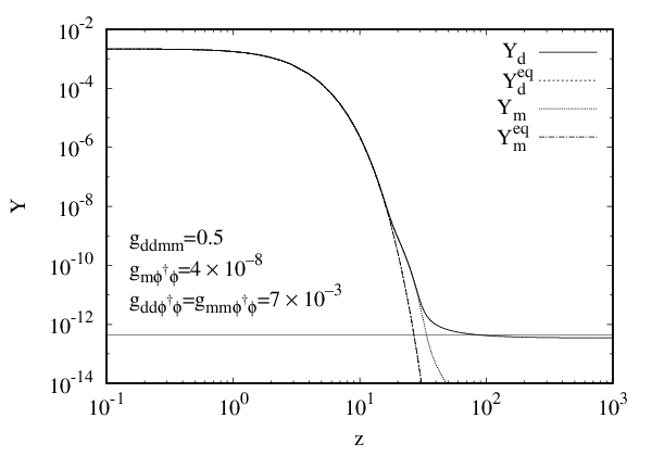
Especially, in the case with sufficiently strong - interaction, the evolutions of the DM density exhibits interesting behavior, i.e., two step DM density decreasing. At the first step, the dark sector chemically decouples from the SM particles, and the DM density is temporarily frozen to a value much higher than usual thermal relic DM scenario (“fake” freeze-out). This is “fake” because the DM particle still interacts with the mediator particle strongly, and it keeps the chemical equilibrium with the mediator. The next step DM density decreasing starts when the mediator decay becomes active. The relic abundance of the DM density is therefore controlled by the mediator life-time. The true freeze-out takes place only after the DM particle decouples from the mediator. The evolution of the DM density thus exhibits characteristic “terrace” structure in this setup as shown in Fig. 2 later.
The realization of the secluded mechanism with opens a new fascinating window on the DM model buildings, allowing unified descriptions for the mediator and the DM in the secluded scenarios. We give a concrete example of unified description of mediator and DM, in which both mediator and DM particles are realized as the pseudo Nambu-Goldstone bosons, in a manner similar to the SIMP scenario. We emphasize that the key process in the secluded DM scenario, i.e., the process of the DM pair annihilation into mediator particles, is provided by the low energy theorem amplitude and is well under theoretical control in our concrete model.
This paper is organized as follows: In Sec. II, we give a toy model of the secluded DM model. A brief review on the Boltzmann equation we use in our numerical analysis is also described there. The results on the numerical computations on the evolutions of the DM and mediator number densities are presented in Sec. III. We then propose a pionic DM scenario based on our numerical computation in Sec. IV. Sec. V is devoted for summary and outlook. We ensure comprehension of the numerical evolutions by analytically describing the relevant quantities in Appendix. A.
II Boltzmann equation in A Toy Model for Secluded Dark Matter
It is possible to write down a toy model in which several known DM density decreasing mechanisms, such as the familiar thermal relic DM, the cannibal DM with a decaying mediator, and the secluded DM with a mass gap , are described in a unified manner. The secluded DM scenario with we consider in this paper can also be implemented in this toy model as well. We here introduce such a toy model and write down the coupled Boltzmann equations governing the evolutions of the DM and the mediator number densities.
II.1 A toy model
We introduce two real scalar fields and , which correspond to the DM and mediator particles and , respectively. They interact with each other and also with the SM weak doublet Higgs field . The model is described by the Lagrangian,
| (II.1) |
with , being masses of the DM particle and the mediator particle , respectively. The longevity of the DM particle is protected by the symmetry .
We know several parameter regions explain the cosmologically observed DM relic abundance in the present toy model.
- •
If we take the much heavier than the DM mass,
we can integrate out the particle in the Lagrangian and we only have two parameters and , which can be chosen to obtain the relic abundance. This model is nothing but the conventional Higgs portal DM [22, 23, 24], a typical scenario in the familiar thermal relic DM.
- •
If we take
and very small , the dark sector particles and decouple from the visible sector almost completely and the thermal equilibrium with the visible sector is lost. For
the mediator decays into the visible particles after the decoupling between and , due to the long life-time of , . In this case, and can be chosen to obtain the observed relic density. This scenario can be considered as a Higgs portal realization of the cannibal DM model [20].
- •
It is also possible to consider a scenario in which both and are non-zero but satisfy
The DM coupling strengths are arranged so as the dark sector to keep its thermal contact with the visible sector even after its chemical decoupling. Similarly to the cannibal DM case, if we take
and non-vanishing , the DM density decreasing process takes place in the scattering process. The coupling and the DM mass control the relic abundance. This possibility (the secluded DM with a large mass gap) has been known since Refs. [18, 19].
Note that the model with and can also accommodate the appropriate DM relic density. See Ref.[25] for a study of this possibility in the stable mediator limit. It will be dealt with further in a separate publication.
In the following sections, we consider yet another realization to obtain the appropriate relic abundance by choosing the life-time of the mediator particle in a novel parameter region and , , which guarantee the thermal equilibrium between the dark sector and SM fields in the epoch of its chemical decoupling from the SM particles.
II.2 Boltzmann equation with a species going out of equilibrium
Here we describe a procedure to obtain the Boltzmann equation for a particle valid even when out-of-chemical-equilibrium particles , and are interacting with the particle . We restrict ourselves to the case in which all of these particles keep kinematical equilibriums with the thermal bath and feel the same temperature . The validity of this assumption in our DM relic density analysis will be discussed later in Sec. III.7.
We illustrate the procedure in a simple setup in which only two processes, (i) decay and inverse decay , (ii) scattering process , are responsible. Using Eq. (5.11) in Ref. [26], the Boltzmann equation for is given by
| (II.2) |
with
| (II.3) |
denoting a Lorentz invariant phase space for . Here stands for the internal degree of freedom for particle . The Hubble rate is given by
| (II.4) |
where represents the total number of relativistic degrees of freedom for particles. We use to simplify the numerical analysis throughout the present paper. The Planck mass is denoted by .
In order to perform the phase space integrals in Eq.(II.2), we assume the distribution functions are approximately given by the Maxwell-Boltzmann distribution form, . Here represents the value of the chemical potential for . The -functions enforce and . Then the distribution functions are rewritten as , and . Note that the number density for a species in chemical equilibrium with the thermal bath is given by
The actual number density for a species out of chemical equilibrium is related with the chemical potential as .
We introduce thermally averaged decay rates and thermally averaged cross sections as follows,
| (II.5) |
| (II.6) |
where is relative velocity of initial particles. The phase space integrals in the Boltzmann equation Eq.(II.2) can now be performed. We obtain
| (II.7) |
which is expressed in terms of the actual number density and the number density in chemical equilibrium . In the case where species and are in chemical equilibrium with the thermal bath, , the Boltzmann equation Eq.(II.7) reduces to a “familiar” form. Once species and/or go out of equilibrium, their number densities deviate from equilibrium values, i.e., , which makes an important difference from the analysis based on the familiar Boltzmann equation. The non-unity ratio can trigger non-equilibration of species even if the rates of the processes and are faster than the Hubble rate .
The assumption we made on the distribution functions cannot be justified if the departures from their chemical and thermal equilibriums are large. It should be noted, however, the validity of this approximation can be guaranteed in the situation in which all of particles , , and start to deviate from their chemical equilibriums almost simultaneously.
II.3 Boltzmann equation for the DM-mediator system
We are now ready to derive the Boltzmann equations which determine the evolutions of the number densities of the DM particle and the mediator particle in our toy model Eq.(II.1). The number changing processes of the DM and the mediator are
| (II.8) |
The interplay between these processes determines the DM relic density.
The Boltzmann equations are derived by implementing the processes (II.8) in (II.7),
| (II.9) |
| (II.10) |
We assumed that the SM Higgs is in chemical equilibrium, i.e, .
Note that, if the mediator couples with the SM particles sizably via or , the mediator keeps its chemical equilibrium with the SM Higgs through the decay and inverse decay process , or through the process. If the chemical equilibrium of the mediator particle lasts until the final DM freeze-out epoch, the mediator can be regarded as a part of background thermal plasma in the process. In this case, the DM relic density is determined almost solely by and becomes insensitive to the values of and .
The situation becomes a bit elaborate, if goes out of chemical equilibrium before decouples from the mediator . All of couplings , and are equally important in the determination of the DM relic abundance in this case.
In the remaining of this section, we analytically derive the critical value of the coupling, which separates these two phases.
We include only the (inverse) decay process in the Boltzmann equation (II.10) as the reaction between the mediator and the SM fields. This simplification is reasonable, because the decay dominates over the scattering with the SM Higgs when the temperature drops below mass. We introduce a variable , where denotes the scale factor of the universe. The Boltzmann equation of can be rewritten in terms of ,
| (II.11) |
where we assumed and keeps their chemical equilibrium. We consider a situation that goes out of equilibrium at a time . at a time ( is an infinitesimal time interval) is obtained by solving the Eq. (II.11) as
| (II.12) |
where is a constant. As long as the inequality
| (II.13) |
is satisfied, immediately goes back to equilibrium. Hence this inequality stands for the equilibrium condition of .
In the derivation of the condition (II.13), we implicitly assume that is constant in an interval . It is necessary for justification for the condition (II.13) to guarantee the inequality in . in is computed as follows,
| (II.14) |
The first term for , where represents the temperature which goes out of equilibrium, is
| (II.15) |
Thus the inequality is rewritten in terms of and as
| (II.16) |
The approximation from the first line to the second line holds for .
As a result, by combining the conditions (II.13) and (II.16), we find the condition to maintain the equilibrium of and the SM fields as
| (II.17) |
We can convert the condition in terms of the model parameters as follows
| (II.18) |
Hence goes out of the equilibrium of and the SM fields for . The non-equilibration of indirectly gives rise to the decoupling from the SM thermal bath via the - scattering. As a result the life-time controls the relic density. We will numerically check these results in next section.
Note that there exist scattering processes with SM fermions or SM gauge bosons, e.g., , , and so on, and they can contribute to the thermalization. These contributions are however negligible. This is understood as follows. As is noted above, key ingredient in our scenario is that goes out of the equilibrium between and SM fields, which leads non-familiar relic density of dark matter. goes out of the equilibrium for . As long as which is minimum value for the thermalization, the reaction dominates over the scatterings processes with SM fermions or SM gauge bosons. Hence we can omit the scattering processes with SM particles via coupling.
III Numerical Results
We here present our results on the numerical computations for the DM relic density.
The evolutions of and particles are illustrated in Sec. III.1,III.2 and Sec. III.3 with numerical results computed at several reference points. We assume in these reference points, since the DM evolution behaves quite differently than the scenario with . Motivated by the unified model of the DM and the mediator, we consider case throughout in this section. We emphasize that all of the results shown below is not affected, however, even if as long as , .
The parameter dependences of the DM relic density are shown in Sec. III.4 and Sec. III.5 assuming . We find that it is necessary to take into account the non-unity ratio in the Boltzmann equations (II.9) and (II.10). The important role of should be emphasized.
In Sec. III.6, we plot the parameter regions consistent with the observed DM relic density in the - plane. Here the mass ratio is denoted by . We find numerically that, if the life-time of the mediator particle is longer than the DM decoupling time from the mediator, the mass ratio cannot exceed in order to account for the observed DM relic abundance. On the other hand, if we introduce a life-time of comparable with or shorter than the DM decoupling time, the situation changes drastically. Our mechanism yields the observed DM relic density in the secluded scenario even for a completely degenerated - system, with which we deduce the upper bound on the mediator life-time.
The validity of the Boltzmann equation Eq.(II.7) in which both , and Higgs are assumed to feel the same temperature is studied in Sec. III.7.
III.1 Evolution example 1


We here give an example of the number density evolutions for the DM and mediator particles. A typical evolution of () is shown in Fig. 2, with () being the number density normalized by the entropy density for (). The horizontal axis shows . The mediator and the DM are assumed to degenerate in mass . We take , , and as a reference point in this plot. The Hubble rate , thermal averaged decay rate and inverse decay rate of ( and ), and interaction rates of , , and are shown in Fig. 2 with the same parameter set. As we see in Fig. 2, there exist characteristic time scales which play important roles in the determination of the evolutions. They are
- (a)
The time scale at which the both DM and mediator go out of chemical equilibrium from the SM thermal bath. We find it is in Fig. 2. This scale can be determined by the condition
(III.1) - (b)
The scale determined by the mediator life-time,
(III.2) The mediator decay starts to affect the evolution of the system after .
- (c)
The time scale until when the detailed balance between the and processes is held. The detailed balance ends at . Due to the rapid decreasing of the mediator density through the mediator decay, the mediator density falls below after . The mediator decay rate exceeds the interaction rate of for . We see with the present set of parameters.
- (d)
The time scale when the interaction rate becomes slower than the Hubble rate. The DM density is frozen to its final abundance after , decoupled from the mediator particle . We find in Fig. 2.
The DM evolution in this setup exhibits distinctive “terrace” structure as shown in Fig. 2, which can be understood step by step in terms of these characteristic time scales.
In the beginning of the evolution (), our scenario traces familiar DM evolution in the Higgs portal DM scenario. The DM is thermalized through the process whose rate is much larger than . The equilibrium between and the background SM fields is also achieved through the process .
At the next stage (), the DM density is temporarily “frozen” to a value () much higher than the corresponding value () in the well-known Higgs portal DM scenario. We call this phenomenon “fake” freeze-out of the DM. The larger value of is because the DM interacts with the SM much weaker than the Higgs portal DM in the present model and thus it decouples from the SM at an earlier time. Note that the mediator goes out of the equilibrium with the SM simultaneously with the DM “fake” freeze-out. This situation holds even in the case due to the sizable interactions among and .
The mediator decay becomes active after . The inverse decay rate , on the other hand, is negligibly small. The density in a comoving volume starts to decrease exponentially after through the mediator decay . The temporarily “frozen” mediator density is then thawed by the mediator decay. We see in Fig. 2, due to the strong interaction , the DM density tracks until . We thus find the DM density decreases drastically after its decoupling from the SM thermal bath. It is important to emphasize that the decoupling of and from the SM thermal bath does not imply the freeze-out of their densities.
Once the decay rate exceeds the interaction rate of , the rapidly-decreasing density breaks the detailed balance between the interactions and . Note that the DM density is still decreasing if the interaction rate of is larger than the Hubble rate . The DM density is fixed to its final abundance only at the last stage () when the interaction rate of becomes smaller than .
III.2 Evolution example 2

Another example of typical evolution is shown in Fig. 4, which differs qualitatively from the example we had shown in the previous subsection. In this plot, we take parameters TeV, , , and , which lead to , , , and as shown in Fig. 4. We therefore find , in contrast to the inequality we had in the previous subsection. As a result, the distinctive “terrace” structure we observed in the previous subsection disappears in Fig. 4. Instead, we see a change of slope at the scale in the plot of .
III.3 Evolution example 3


Here we give an example in which the mediator decay time scale coincides approximately with the DM decoupling scale . This situation happens with parameters TeV, , , and . Corresponding time scales are , , , and . See Fig. 6 and Fig. 6 for the behavior of evolution and interaction rates, respectively. The mediator decay affects the evolution immediately after the DM decoupling from the SM thermal bath. We see no clear terrace structure nor simple slope-change in the DM evolution shown in Fig. 6.
III.4 dependence


We study the dependence of the relic density. Fig. 7 shows the DM relic density as a function of . We take . Parameters taken for the analysis are , , , , , and , respectively.
Larger provides smaller relic density. This is because longer equilibrium between and can be achieved by larger , which delays the decoupling between and . As we show in Appendix A, the semi-analytic formula (A.31) for the DM relic abundance is actually inversely proportional to and supports this understanding.
On the other hand, smaller gives larger relic density. For each value of , the relic density approaches to its asymptotic value in the - collision-less limit, which corresponds to the DM relic density controlled by the in the Higgs portal scenario. The DM relic density becomes almost insensitive to the value of for . This is understood as follows. Fig. 8 shows the interaction rates of and for , and . Other coupling strengths are taken as and . We see the DM-mediator decoupling epoch () is earlier than the DM-Higgs decoupling () for . There is therefore no dependence of the relic density for .
Hence, our mechanism to reduce the DM relic density works only when the coupling is stronger than the DM-Higgs coupling in the Higgs portal DM scenario.
III.5 Mediator life-time dependence

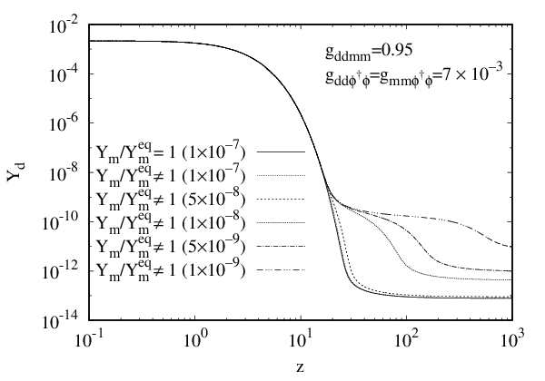
If the mediator were in chemical equilibrium with the thermal bath, and thus . The DM Boltzmann equation (II.9) would then be separated from the mediator Boltzmann equation (II.10) completely. The DM relic abundance would therefore be insensitive to the mediator properties such as the mediator life-time ( coupling). In the reality, however, the mediator departs from its chemical equilibrium almost simultaneously with the “fake” freeze-out epoch of the DM. We need to take into account effects of in our computations of the DM relic density. Solving the coupled Boltzmann equations (II.9) and (II.10), we obtain the DM relic density as plotted in the solid line in Fig. 9 as a function of . On the other hand, if the chemical equilibrium of the mediator particle were satisfied in (II.9), we would obtain the dotted line result in Fig. 9. We see the coupling controls the DM relic density. The effects of the departure of the mediator chemical equilibrium are significant.
The relic density decreases with decreasing life-time (increasing ). It approaches to the value of around . The behavior of the relic density is understood as follows. For as derived in Eq. (II.18), the mediator keeps its chemical equilibrium with the SM Higgs. The density in (quasi-)equilibrium exponentially drops, and guides the over-abundant density to the observed one.
Fig. 10 shows the evolutions of for each . Too long life-time keeps over-densities of for a long period, and leads to a mild damping of . Freeze-out of occurs at large due to a large deviation of from unity, and hence remains over-abundant. On the other hand, a deviation of from unity becomes smaller for shorter life-time. The Boltzmann equations (II.9) and (II.10) and the relic density approach to those in familiar thermal relic scenarios.
We here note the non-unities and also affect the evolutions of the and densities after the epoch , when the detailed balance of the process is broken.
III.6 Parameter regions consistent with the observed DM relic abundance

We show parameters that can account for the central value of the observed DM relic density in Fig. 11. We take TeV and . The solid, dashed and dotted lines correspond to the case of negligibly small (very late-time decaying mediator), and , respectively. We see in this plot that for the coupling required for the observed relic density gets close to an asymptotic value , almost independently of . This illustrates the fact that in secluded scenarios with a light mediator (), the DM relic density is controlled only by and the DM mass , and becomes insensitive to and .
On the other hand, as gets larger, the required coupling also becomes larger. For the case of the negligibly small (the very late time decaying mediator), especially, the coupling goes over the unitarity bound around . We thus find the upper bound on so as to explain the observed DM relic density. Thus, with the extremely long-lived mediator which survives even after the DM decoupling from the mediator, the completely degenerated mediator setup () is not feasible to account for the observed DM relic density. This property is consistent with the numerical results for the DM relic abundance done in the context of a right-handed sneutrino-neutrino DM-mediator model[27].
The situation changes drastically if we consider a shorter life-time mediator. The secluded DM scenario with becomes viable if the mediator life-time is comparable with or shorter than the DM decoupling time from the mediator. Actually, when , the coupling is required at and is marginally consistent with the unitarity. For the mediator with shorter life-time (larger ), it is easier to find the parameter regions consistent with the observed relic density and also with the unitarity. We numerically obtain the lower limit on , for TeV and .
The required coupling for decreases with increasing . It approaches to an asymptotic value around . This is because for , as is described in Section II.3, the mediator is thermalized through the decay and inverse decay process, , and remains in chemical equilibrium with the SM sector until the final freeze-out of the DM number density. In this case, the DM relic density is insensitive to and , and is determined almost through the DM mass , the DM-mediator mass ratio and the - coupling .
III.7 Temperature of - system

Throughout this work, we assume that the temperatures of - system holds on the background temperature even after they decouple from the SM particles.
Kinetic equilibrium of and the SM fields ensures that they evolve in a common background with a temperature, even if the chemical equilibrium of them is not achieved. Fig. 12 shows the comparison of the Hubble expansion rate and the interaction rate of . We take , , and . The interaction rate dominates in the region of . For , on the other hand, the dark sector evolves in the temperature which may be different from the SM temperature .
In the example 1 shown in Sec. III.1, does not hold after the mediator life-time scale . The two-step DM density decreasing profile (“terrace” behavior) is maintained even if we take into account the effects of , though we neglected the effects in our numerical computations in this paper. The issue will be discussed further in our future publication.
It is also possible to modify our toy model to keep for a longer period, assuming, e.g., the neutrino portal couplings for the dark sector instead of the Higgs portal coupling.
IV A Realization in Pionic Dark Matter Scenario
As we have shown in the previous section, the scattering amplitude needs to be strong enough to achieve the observed DM relic density in our degenerated mediator setup. If we assume the DM and mediator particles are elementary, it is extremely difficult to obtain such a strong interaction without conflicting with the Landau pole problem, however. We here show both of the degeneracy between the DM particle () and the mediator particle (), , and the marginally strong interaction in scattering can be accommodated in models of dark strong dynamics having the dark pions [28, 29, 30] as composite particles. Note the dark pions exist ubiquitously in models of electroweak symmetry breaking, including technicolor[31], composite Higgs[32, 33] and also in classically scale invariant extentions of the SM[34, 35, 36, 37]. Note also the SIMP mechanism [14, 15, 38] is embedded in the dark pion scenario, although the DM relic density decreasing mechanism presented in this paper does not rely on it.
IV.1 Dark QCD and Dark Pions
We consider a model in which both DM particle and mediator are unified in a dark pion multiplet. The dark pions are hypothetical pseudo Nambu-Goldstone bosons associated with dynamical breaking of a newly introduced dark chiral symmetry. They often are the lightest BSM particle existing in models with a dark strong dynamics (dark QCD), and are regarded as the DM candidate particles. In this section, we show the - unification and the marginally strong amplitude can be achieved in a setup with the dark pions.
We introduce a new strong Yang-Mills gauge dynamics, termed “dark QCD” as,
| (IV.1) |
in analog to the usual quantum chromodynamics (QCD). Here the dark quark fermion field forms a dark isospin doublet
| (IV.2) |
and belongs to the fundamental representation of the dark QCD gauge group. The fermion fields with left- and right-handed chiralities are specified by using subscripts and , respectively. The Lagrangian Eq.(IV.1) enjoys global dark chiral symmetry,
| (IV.10) | |||
with being the Pauli matrix. In the Lagrangian Eq.(IV.1), the dark gluon field couples with the dark quark through the covariant derivative,
| (IV.19) |
with being the fundamental representation matrix of the dark QCD gauge symmetry. The dark gluon field strength is defined as usual
| (IV.20) |
Note here that both the dark fermion and the dark gluon are blind to the SM gauge group. These fields therefore contribute to the dark component in the universe.
The negative beta function in the Yang-Mills theory renormalization group equations makes the dark QCD gauge coupling strength non-perturbatively strong and induces very strong attractive force between and , which triggers a condensate
| (IV.21) |
and dynamical breaking of the dark chiral symmetry,
| (IV.22) |
in a manner similar to the usual QCD.
It is now apparent how dark pions () appear in this setup. They are the Nambu-Goldstone bosons associated with the dynamical symmetry breaking Eq.(IV.22). Due to the exact chiral symmetry, however, the dark pions remain exactly massless in this model. We therefore introduce explicit symmetry breaking terms,
| (IV.23) |
with denoting the doublet SM Higgs field. The explicit breaking terms Eq.(IV.23) make the dark pions massive. The dark pions interact with the SM Higgs field also through the explicit breaking terms Eq.(IV.23). Possible origin of these explicit symmetry violating terms Eq.(IV.23) will be dealt in the next subsection in a renormalizable field theory framework. In this subsection, we concentrate on the impacts of these terms in the dark pion phenomenologies.
The dark pion low energy effective theory can be described by using the chiral Lagrangian,
| (IV.24) |
with being the dark pion decay constant. Here the non-linear chiral field is expressed using the dark pion field ,
| (IV.25) |
The effects of the explicit violation of the dark chiral symmetry, Eq.(IV.23), can be analyzed by using
| (IV.26) |
with being a low energy constant related with the dark quark pair condensate.
Expanding the chiral Lagrangian Eq.(IV.24) in terms of the dark pion field , we obtain
| (IV.27) | |||||
It should be noted here that all of the dark pions , , share the identical mass , which can be evaluated by using the low energy constant and the dark quark mass ,
| (IV.28) |
We also find the dark pions couple with the SM Higgs boson through Eq.(IV.23) as,
| (IV.29) |
which plays an important role to thermalize the dark pions in the early universe.
Note that the Lagrangians Eq.(IV.1) and Eq.(IV.23) are invariant under the fermion transformation,
| (IV.30) |
which also survives as an exact symmetry even after the dynamical chiral symmetry breaking. It is easy to see that and are odd under the transformation Eq.(IV.30)
| (IV.31) |
They are therefore stable and can be considered as the DM candidate particles. On the other hand, the third component of the dark pion is even under the symmetry Eq.(IV.30). It then decays into the SM Higgs bosons through the coupling
| (IV.32) |
We identify the third component dark pion as the mediator in the secluded DM scenario. In this manner, the DM and the mediator particles are unified in the same dark isospin multiplet. The dark pion scattering amplitude can be evaluated by using the low energy theorem,
| (IV.33) | |||||
The amplitude Eq.(IV.33) is strong enough to make the secluded DM scenario based on this setup. If we deduce the interaction coupling of Eq. (II.1) from the amplitude at the threshold, we obtain
| (IV.34) |
The marginally strong amplitude can thus be easily achieved for the massive dark pions with . The other phenomenological couplings , and are
| (IV.35) |
Note that the dark baryons also potentially contribute to the DM relic abundance in this model. The dark baryon relic abundance turns out, however, to be negligibly small in its minimal setup of the dark QCD at the TeV scale, as demonstrated in the techni-baryon context in Ref. [39]. In models of asymmetric dark baryon DM, our mechanism to decrease the dark pion number density can be applied to make the dark pions harmless in the cosmology[40, 41].
IV.2 A UV completion
The purpose of this subsection is to give a possible renormalizable UV completion behind the explicit breaking terms Eq.(IV.23). For such a purpose, we introduce real scalar fields and , which interact with the dark fermions through the Yukawa Lagrangian
| (IV.36) |
with being the Yukawa coupling strength. Note that the Yukawa Lagrangian violates explicitly the symmetry down to .
We introduce kinetic and potential terms for these scalar field in a renormalizable manner,
| (IV.37) |
with
with being a constant with a mass dimension. We also introduce the interaction among , and the SM Higgs field as
| (IV.39) |
Note that the dimension 4 operators in the potential Eq.() and the interaction with the SM Higgs Eq.(IV.39) respect the symmetry among and , while the operators with lower dimensions violate the symmetry. The dimension 2 operators respect the symmetries , , while the dimension 1 operators do not. The potential is arranged to give non-vanishing vacuum expectation values (VEVs) for (and ) around the scale. It is convenient if we parametrize VEVs as
| (IV.40) |
We also rewrite the explicit symmetry violating parameters and using new parameters and ,
| (IV.41) |
Note here that, if we take , the angle is determined as
| (IV.42) |
with taking an integer value. Much involved vacuum structure than Eq.(IV.42) can be obtained if we take non-trivial value of . Especially, in this case, the mass eigenstates arising from and fields do not necessary align to the VEV direction. The misalignment between the VEVs and the particle mass eigenstates causes interesting phenomenologies in this setup.
It is a bit tedious but straightforward to obtain the low energy effective theory by integrating out the and fields around the vacuum at the tree-level. Due to the complex structure of the vacuum Eq.(IV.40), the dark quarks acquire a complex mass in general, which can be rotated away by performing an appropriate chiral rotation in the dark quark fields.
Hereafter, we take
| (IV.43) |
| (IV.44) |
Fig. 13 shows the behaviour of
| (IV.45) |
We see it is possible to take sufficiently large value of , if we take the parameter small enough. Note that a symmetry ( symmetry) is restored in the limit. The smallness of coupling ( coupling), as we assumed in our numerical demonstrations of Sec. III, can thus be explained in a technically natural manner by the smallness of the parameter.

V Summary and Outlook
We have demonstrated in this article that the secluded DM scenario can successfully explain the observed relic DM density in the universe even in the case with the non-negligibly heavy mediator particle compared with the dark matter particle mass, , if the mediator life-time is short enough and the transition occurs rapidly enough. The assumption imposed in the original secluded DM scenario[18, 19] is therefore not necessarily required. Allowing a heavy mediator having the mass nearly degenerate with the dark matter particle mass , novel possibilities of particle theory DM model buildings are now opened. We gave a concrete renormalizable DM model, in which both the dark matter particle and the mediator particle are realized as the dark triplet pseudo Nambu-Goldstone particles produced in the dark chiral symmetry breaking in the dark QCD. The rapid transition required in this scenario is naturally achieved thanks to the compositeness of the dark pions ( and ) and the dark strong dynamics.
Although we concentrated on the computations of the relic abundance in this manuscript, much work need to be done in the DM phenomenologies in this scenario. Due to the smallness of the DM coupling with the SM sector, the direct detection of the secluded DM and the production of the DM particles in the high energy collider experiments become rather challenging. The large amplitude and the subsequent decay of the mediator particle , on the other hand, induce interesting signals in the indirect astrophysical DM detection experiments. The dark pion model we proposed in this paper can easily incorporate the DM particle number decreasing mechanism through the scattering via the WZW interaction (SIMP mechanism) in addition to the DM number decreasing from the mediator decay. These issues will be discussed in a separate publication.
Note added
Acknowledgements
We thank Fumihiro Takayama, Paolo Gondolo and Shigeki Matsumoto for useful discussions and valuable comments. This work is supported in part by the JSPS Grant-in-Aid for Scientific Research 15K05047 (M.T.) and 16K05325 and 16K17693 (M.Y.).
Appendix A Terrace structure studied in a semi-analytic manner
In this appendix, we study the terrace structure we numerically found in Sec.III.1 more closely using an analytic method. A semi-analytic formula to evaluate the DM relic abundance is also given. We assume the mediator and the DM degenerate in mass, , as in Sec.III.1. They also possess the same size couplings with the SM Higgs field, , thus . The total number of relativistic degrees of freedom is taken to be .
We first consider the fake freeze-out, the decoupling of the DM-mediator system from the SM particles. Since the mediator decay process is not active at the fake freeze-out time scale, we can neglect the term in the Boltzmann equation (II.10). We also know , () and the Boltzmann equation describing the fake freeze-out behavior can be written as
| (A.1) |
with
| (A.2) |
The Boltzmann equation (A.1) can be converted to a form
| (A.3) |
with is defined as
| (A.4) |
Here and are number densities normalized by entropy density , and The thermal equilibrium and are
| (A.5) |
with
| (A.6) |
We therefore obtain
| (A.7) |
The coefficient in Eq.(A.3) comes from the cross section,
| (A.8) | |||||
Here is defined through
| (A.9) |
Note that the process ( process) occurs through the -wave. We therefore use in our numerical estimates.
The freeze-out phenomenon in the type of Boltzmann equation (A.3) has been extensively studied in the textbook [26]. We here only quote the results. The time-scale at which starts to exhibit the fake freeze-out behavior () can be defined by
| (A.10) |
with being an order constant. It can be evaluated as
The textbook suggests gives the best fit. Using this value of , and the set of parameters in the evolution example 1, we obtain
| (A.12) |
which agrees with the fake freeze-out time scale shown in Fig. 2.
We next move to the final (true) freeze-out when the DM decouples from the mediator. Note that the mediator decay is already active at the age of the final freeze-out. The term in Eq.(II.10) thus plays an important role. On the other hand, the and are negligibly small. The Boltzmann equations can be approximated as
| (A.13) | |||||
Here we used . The coefficients and are defined as
| (A.15) | |||||
| (A.16) |
We define as
| (A.17) |
We should note here that in the process depends on the velocity linearly in the case of - mass degeneracy. The parameter in the Boltzmann equations (A.13) and () should therefore be [44].
Summing up (A.13) and (), we obtain
| (A.18) |
Note also that tracks very closely until the final freeze-out , and thus
| (A.19) |
Eq.(A.18) can be solved as
| (A.20) |
for . Here denotes the integral constant. We assume further that the behavior is valid even at and solve the Boltzmann equation in the form of
| (A.21) |
with
| (A.22) |
instead of its original form (A.13). The integral constant is determined by fitting Eq.(A.20) with the numerical solution around . It can also be determined roughly through matching with the epoch physics as we will show later.
The freeze-out phenomenon in Eq.(A.21) can now be analyzed in a manner similar to the textbook calculation of the standard cold thermal relic abundance. There are a couple of important differences in (A.21), however: the fractional and the damping behavior of . We see in below how these differences affect the freeze-out phenomenon in (A.21).
We introduce
| (A.23) |
and define the freeze-out time scale by
| (A.24) |
with being an order constant. The Boltzmann equation (A.21) can be expressed as
| (A.25) |
which can be solved approximately at as
| (A.26) | |||||
Comparing Eq.(A.26) with Eq.(A.24), we obtain
| (A.27) |
which leads to a formula to determine the freeze-out time scale
| (A.28) | |||||
Note is proportional to in Eq.(A.28). This is in contrast to the usual cold thermal relic computation in which is proportional to . This property comes from the damping behavior of in this scenario. We also note very slow convergence of the series expansion Eq.(A.28). In our numerical anslysis, we therefore use Eq.(A.27) directly, rather than Eq.(A.28).
Once we determine , we can compute the relic abundance at by
| (A.29) |
For , (A.25) can be approximated as
| (A.30) |
Integrating (A.30) from to , we obtain
| (A.31) |
Here the initial value uncertainty () is absorbed in the uncertainty in . Note (A.31) is identical to the textbook formula for the cold thermal relic abundance, except for the fractional value of . We obtain and in our numerical analysis presented in Sec. III.1. Using these values, we see Eq.(A.31) as combined with (A.28) gives the best fit with
| (A.32) |
which is perfectly consistent with the assumption we made on : it is an order constant. The corresponding freeze-out is calculated as
| (A.33) |
The final task we need to carry out is to make a relation between the fake freeze-out and the final freeze-out . This can be done by computing the coefficient in (A.20) in terms of . Assuming the textbook formula
| (A.34) |
gives the abundance at in Eq.(A.20), we see
| (A.35) |
Eq.(A.35) gives a result consistent with our numerical fit on within 40% uncertainty.
References
- [1] K. A. Olive et al. [Particle Data Group Collaboration], “Review of Particle Physics,” Chin. Phys. C 38 (2014) 090001. doi:10.1088/1674-1137/38/9/090001
- [2] G. Hinshaw et al. [WMAP Collaboration], “Nine-Year Wilkinson Microwave Anisotropy Probe (WMAP) Observations: Cosmological Parameter Results,” Astrophys. J. Suppl. 208 (2013) 19 doi:10.1088/0067-0049/208/2/19 [arXiv:1212.5226 [astro-ph.CO]].
- [3] P. A. R. Ade et al. [Planck Collaboration], “Planck 2015 results. XIII. Cosmological parameters,” arXiv:1502.01589 [astro-ph.CO].
- [4] G. Bertone, D. Hooper and J. Silk, “Particle dark matter: Evidence, candidates and constraints,” Phys. Rept. 405 (2005) 279 doi:10.1016/j.physrep.2004.08.031 [hep-ph/0404175].
- [5] J. L. Feng, “Dark Matter Candidates from Particle Physics and Methods of Detection,” Ann. Rev. Astron. Astrophys. 48 (2010) 495 doi:10.1146/annurev-astro-082708-101659 [arXiv:1003.0904 [astro-ph.CO]].
- [6] B. W. Lee and S. Weinberg, “Cosmological Lower Bound on Heavy Neutrino Masses,” Phys. Rev. Lett. 39 (1977) 165. doi:10.1103/PhysRevLett.39.165
- [7] T. Marrodán Undagoitia and L. Rauch, “Dark matter direct-detection experiments,” J. Phys. G 43 (2016) no.1, 013001 doi:10.1088/0954-3899/43/1/013001 [arXiv:1509.08767 [physics.ins-det]].
- [8] D. Abercrombie et al., “Dark Matter Benchmark Models for Early LHC Run-2 Searches: Report of the ATLAS/CMS Dark Matter Forum,” arXiv:1507.00966 [hep-ex].
- [9] A. Tan et al. [PandaX-II Collaboration], “Dark Matter Results from First 98.7 Days of Data from the PandaX-II Experiment,” Phys. Rev. Lett. 117 (2016) no.12, 121303 doi:10.1103/PhysRevLett.117.121303 [arXiv:1607.07400 [hep-ex]].
- [10] A. Manalaysay, “Dark-matter results from 332 new live days of LUX data,” talk presented at IDM2016, The University of Sheffield, Sheffiled, UK, July 21, 2016.
- [11] D. S. Akerib et al., “Results from a search for dark matter in the complete LUX exposure,” arXiv:1608.07648 [astro-ph.CO].
- [12] P. Agnes et al. [DarkSide Collaboration], “Results from the first use of low radioactivity argon in a dark matter search,” Phys. Rev. D 93 (2016) no.8, 081101 doi:10.1103/PhysRevD.93.081101 [arXiv:1510.00702 [astro-ph.CO]].
- [13] R. Agnese et al. [SuperCDMS Collaboration], “Improved WIMP-search reach of the CDMS II germanium data,” Phys. Rev. D 92 (2015) no.7, 072003 doi:10.1103/PhysRevD.92.072003 [arXiv:1504.05871 [hep-ex]].
- [14] Y. Hochberg, E. Kuflik, T. Volansky and J. G. Wacker, “Mechanism for Thermal Relic Dark Matter of Strongly Interacting Massive Particles,” Phys. Rev. Lett. 113 (2014) 171301 doi:10.1103/PhysRevLett.113.171301 [arXiv:1402.5143 [hep-ph]].
- [15] Y. Hochberg, E. Kuflik, H. Murayama, T. Volansky and J. G. Wacker, “Model for Thermal Relic Dark Matter of Strongly Interacting Massive Particles,” Phys. Rev. Lett. 115 (2015) no.2, 021301 doi:10.1103/PhysRevLett.115.021301 [arXiv:1411.3727 [hep-ph]].
- [16] J. Wess and B. Zumino, “Consequences of anomalous Ward identities,” Phys. Lett. B 37 (1971) 95. doi:10.1016/0370-2693(71)90582-X
- [17] E. Witten, “Global Aspects of Current Algebra,” Nucl. Phys. B 223 (1983) 422. doi:10.1016/0550-3213(83)90063-9
- [18] M. Pospelov, A. Ritz and M. B. Voloshin, “Secluded WIMP Dark Matter,” Phys. Lett. B 662 (2008) 53 doi:10.1016/j.physletb.2008.02.052 [arXiv:0711.4866 [hep-ph]].
- [19] N. Arkani-Hamed, D. P. Finkbeiner, T. R. Slatyer and N. Weiner, “A Theory of Dark Matter,” Phys. Rev. D 79 (2009) 015014 doi:10.1103/PhysRevD.79.015014 [arXiv:0810.0713 [hep-ph]].
- [20] D. Pappadopulo, J. T. Ruderman and G. Trevisan, “Dark matter freeze-out in a nonrelativistic sector,” Phys. Rev. D 94 (2016) no.3, 035005 doi:10.1103/PhysRevD.94.035005 [arXiv:1602.04219 [hep-ph]].
- [21] A. Berlin, D. Hooper and G. Krnjaic, “PeV-Scale Dark Matter as a Thermal Relic of a Decoupled Sector,” Phys. Lett. B 760 (2016) 106 doi:10.1016/j.physletb.2016.06.037 [arXiv:1602.08490 [hep-ph]].
- [22] V. Silveira and A. Zee, “Scalar Phantoms,” Phys. Lett. B 161 (1985) 136. doi:10.1016/0370-2693(85)90624-0
- [23] J. McDonald, “Gauge singlet scalars as cold dark matter,” Phys. Rev. D 50 (1994) 3637 doi:10.1103/PhysRevD.50.3637 [hep-ph/0702143 [HEP-PH]].
- [24] C. P. Burgess, M. Pospelov and T. ter Veldhuis, “The Minimal model of nonbaryonic dark matter: A Singlet scalar,” Nucl. Phys. B 619 (2001) 709 doi:10.1016/S0550-3213(01)00513-2 [hep-ph/0011335].
- [25] G. Belanger and J. C. Park, “Assisted freeze-out,” JCAP 1203 (2012) 038 doi:10.1088/1475-7516/2012/03/038 [arXiv:1112.4491 [hep-ph]].
- [26] E. W. Kolb and M. S. Turner, “The Early Universe,” Front. Phys. 69, 1 (1990).
- [27] P. Bandyopadhyay, E. J. Chun and J. C. Park, “Right-handed sneutrino dark matter in seesaw models and its signatures at the LHC,” JHEP 1106 (2011) 129 doi:10.1007/JHEP06(2011)129 [arXiv:1105.1652 [hep-ph]].
- [28] Y. Bai and R. J. Hill, “Weakly Interacting Stable Pions,” Phys. Rev. D 82 (2010) 111701 doi:10.1103/PhysRevD.82.111701 [arXiv:1005.0008 [hep-ph]].
- [29] M. R. Buckley and E. T. Neil, “Thermal dark matter from a confining sector,” Phys. Rev. D 87 (2013) no.4, 043510 doi:10.1103/PhysRevD.87.043510 [arXiv:1209.6054 [hep-ph]].
- [30] S. Bhattacharya, B. Melić and J. Wudka, “Pionic Dark Matter,” JHEP 1402 (2014) 115 doi:10.1007/JHEP02(2014)115 [arXiv:1307.2647 [hep-ph]].
- [31] T. A. Ryttov and F. Sannino, “Ultra Minimal Technicolor and its Dark Matter TIMP,” Phys. Rev. D 78 (2008) 115010 doi:10.1103/PhysRevD.78.115010 [arXiv:0809.0713 [hep-ph]].
- [32] M. Frigerio, A. Pomarol, F. Riva and A. Urbano, “Composite Scalar Dark Matter,” JHEP 1207 (2012) 015 doi:10.1007/JHEP07(2012)015 [arXiv:1204.2808 [hep-ph]].
- [33] A. Carmona and M. Chala, “Composite Dark Sectors,” JHEP 1506 (2015) 105 doi:10.1007/JHEP06(2015)105 [arXiv:1504.00332 [hep-ph]].
- [34] T. Hur and P. Ko, “Scale invariant extension of the standard model with strongly interacting hidden sector,” Phys. Rev. Lett. 106 (2011) 141802 doi:10.1103/PhysRevLett.106.141802 [arXiv:1103.2571 [hep-ph]].
- [35] Y. Ametani, M. Aoki, H. Goto and J. Kubo, “Nambu-Goldstone Dark Matter in a Scale Invariant Bright Hidden Sector,” Phys. Rev. D 91 (2015) no.11, 115007 doi:10.1103/PhysRevD.91.115007 [arXiv:1505.00128 [hep-ph]].
- [36] H. Hatanaka, D. W. Jung and P. Ko, “AdS/QCD approach to the scale invariant extension of the standard model with a strongly interacting hidden sector,” arXiv:1606.02969 [hep-ph].
- [37] M. Holthausen, J. Kubo, K. S. Lim and M. Lindner, “Electroweak and Conformal Symmetry Breaking by a Strongly Coupled Hidden Sector,” JHEP 1312 (2013) 076 doi:10.1007/JHEP12(2013)076 [arXiv:1310.4423 [hep-ph]].
- [38] Y. Hochberg, E. Kuflik and H. Murayama, “SIMP Spectroscopy,” JHEP 1605 (2016) 090 doi:10.1007/JHEP05(2016)090 [arXiv:1512.07917 [hep-ph]].
- [39] R. S. Chivukula and T. P. Walker, “Technicolor Cosmology,” Nucl. Phys. B 329 (1990) 445. doi:10.1016/0550-3213(90)90151-3
- [40] M. Farina, “Asymmetric Twin Dark Matter,” JCAP 1511 (2015) no.11, 017 doi:10.1088/1475-7516/2015/11/017 [arXiv:1506.03520 [hep-ph]].
- [41] M. Freytsis, S. Knapen, D. J. Robinson and Y. Tsai, “Gamma-rays from Dark Showers with Twin Higgs Models,” JHEP 1605 (2016) 018 doi:10.1007/JHEP05(2016)018 [arXiv:1601.07556 [hep-ph]].
- [42] M. Farina, D. Pappadopulo, J. T. Ruderman and G. Trevisan, “Phases of Cannibal Dark Matter,” JHEP 1612 (2016) 039 doi:10.1007/JHEP12(2016)039 [arXiv:1607.03108 [hep-ph]].
- [43] J. A. Dror, E. Kuflik and W. H. Ng, “Co-Decaying Dark Matter,” Phys. Rev. Lett. 117 (2016) no.21, 211801 doi:10.1103/PhysRevLett.117.211801 [arXiv:1607.03110 [hep-ph]].
- [44] K. Griest and D. Seckel, “Three exceptions in the calculation of relic abundances,” Phys. Rev. D 43 (1991) 3191. doi:10.1103/PhysRevD.43.3191