Entire solutions of superlinear problems with indefinite weights and Hardy potentials.
Abstract
We provide the structure of regular/singular fast/slow decay radially symmetric solutions for a class of superlinear elliptic equations with an indefinite weight on the nonlinearity . In particular we are interested in the case where is positive in a ball and negative outside, or in the reversed situation. We extend the approach to elliptic equations in presence of Hardy potentials. By the use of Fowler transformation we study the corresponding dynamical systems, presenting the construction of invariant manifolds when the global existence of solutions is not ensured.
Key Words: supercritical equations, Hardy potentials, radial
solutions, regular/singular ground
states, Fowler transformation, invariant manifold, continuability.
MR (2010) Subject Classification: 35j75, 35j91, 37d10, 34c37.
1 Introduction
A first purpose of this paper is to study the properties of radial solutions for equations of the form
| (L) |
where , , , and is a differentiable function which is null for and super-linear in . Since we just deal with radial solutions we will indeed consider the following singular ordinary differential equation
| (Lr) |
where, abusing the notation, we have set for , and ′ denotes differentiation with respect to .
Radial solutions play a key role for (L), since in many cases, e.g. , positive solutions have to be radial (but also in many situations in which is allowed to vary, see e.g. [5, 26, 31]). They are also crucial to determine the threshold between fading and blowing up initial data in the associated parabolic problem, see e.g. [14, 39].
In this article we are mainly interested in classifying positive and nodal solutions when is negative for small and positive for large, or in the opposite situation. The prototype for the nonlinearity we are interested in takes the form:
| (1.1) |
where is a continuous function, which is either negative in a ball and positive outside and , or we have the reversed sign condition and , where , are respectively the Serrin and the Sobolev critical exponents.
The behavior of solutions of (Lr), with as in (1.1), changes drastically according to the sign of , when . When for any , positive solutions are convex, and their maximal interval of continuation may be bounded either from above or from below or both. On the other hand if all the solutions of (Lr) are continuable for any ; further, if the structure of positive solutions of (Lr) changes drastically when the exponent in (1.1) passes through some critical values, such as and , see e.g. [20, 35]. In fact new and more complex situations arise when the non-linearity exhibits both subcritical an supercritical behavior with respect to these exponents, see e.g. [3, 4, 5, 23, 24, 40], for a far from being exhaustive bibliography. In fact we have an interaction between the exponent and the asymptotic behavior of . Roughly speaking, if is of type (1.1) and behaves like a positive power, then the critical exponents get smaller, while they get larger if behaves like a negative power. E.g., if then the Sobolev critical exponent becomes .
With very weak assumptions, definitively positive solutions exhibit two behaviors as and as when . Namely may be a regular solution, i.e. and , or a singular solution, i.e. ; a fast decay (f.d.) solution, i.e. , or a slow decay (s.d.) solution, i.e. . We emphasize that in many situations the behavior of singular and slow decay solutions can be specified better (cf. Remark 2.6).
In the whole paper we use the following notation: we denote by the regular solution of (Lr) such that , and by the fast decay solution such that . Moreover we call ground states (G.S.), regular positive solutions defined for any and such that , and singular ground states (S.G.S.) positive singular solutions defined for any and such that , .
In this paper we continue the discussion, begun with [25], which is mainly focused on the case where is of type (1.1), , is discontinuous and equals inside a ball and outside. This kind of equation is a special reaction-diffusion equation, where the reaction, modeled by , is assumed to have a source effect inside a ball and an absorption effect outside. So it can describe, e.g., the temperature in presence of a nonlinear reaction producing energy (taking place in a bounded box) and its inverse absorbing it (taking place in the environment where the box is immersed), both heat regulated. As specified in [25] it can also describe the density of a substance subject to diffusion and to a nonlinear reaction and its inverse, see also [34, §7]. The inhomogeneity may be induced by the presence of an activator or an inhibitor.
In [25] the purpose was to prove existence and exact multiplicity for regular solutions with f.d. and with s.d., and to deduce their nodal properties, but just for a very specific example, discontinuous in .
Here we want to show that the case described in [25] is the prototype for a large class of nonlinearities . So we relax the requirement on ; in particular we assume it to be smooth, and we extend the results to a wider family of potentials , whose main representative is given by
| (1.2) |
where changes sign one time: in particular if , if , for a certain . Section 4 will be devoted to a deeper analysis of the possible nonlinearities we can deal with, but we wish to emphasize that our result is new for this kind of nonlinearity, too.
We emphasize that the presence of G.S. with f.d. is due to the coexistence of source and absorption effects (i.e. changes sign). In literature there are many results on the structure of radial solutions for Laplace equations with indefinite weights , see e.g. [1, 4, 7]. However, these papers are concerned with phenomena which are found when is a positive function, and which persist even if becomes negative in some regions. The structure results we find can just take place if we have a change in the sign of : if is either smaller or larger than there are no G.S. with fast decay, neither if , nor if . In fact, the structure of the solutions of (Lr) described in Corollaries 1.2 and 1.3, reminds of the situation in which and we have a positive which behaves like a positive power for small and a negative power for large, see e.g. [13, 40]. In the same direction goes [6], which proves existence results (using a variational approach) which hold just when the nonlinearities have sign-changing weights; however in [6] the authors consider bounded domains and just in the subcritical case. Further in [15, 32, 33] and in references therein the reader can find several nice and sharp structure results for sign-changing nonlinearities, even for more general operators (-Laplace, relativistic and mean curvature), in the framework of oscillation (and non-oscillation) theory, but for exterior domains, i.e. for solutions defined, say for .
Performing this generalization with respect to [25] we pay two prizes: firstly we can just give existence and multiplicity results, but we lose the control of uniqueness and exact multiplicity since we mainly ask for asymptotic conditions; secondly we have to face many technical problems and the discussion is more involved. The major one is the following: asking for to be negative and possibly superlinear for large, we allow the existence of non-continuable solutions, whose presence causes almost no difficulties for the special nonlinearities considered in [25], but it is a crucial problem here.
In fact the presence of non-continuable solutions, which are typical for the nonlinearity considered, rises a challenging problem from the theoretical point of view. In fact we cannot apply the already established invariant manifold theory for non-autonomous systems (see e.g. [10, 12, 27]). In the appendix we perform a first step in order to extend this theory to the case where non-continuable solutions are allowed. As far as we are aware this is the first time where such a problem is considered, and we think this can be a contribution from a methodological point of view to invariant manifold theory for non-autonomous dynamical systems.
Our analysis is directly performed for the following more general differential equation
| (H) |
and for its radial counterpart
| (Hr) |
We assume that is a differentiable function satisfying the following requirement, which will be assumed in the whole paper:
The introduction in Laplace equation of the additional term , often referred to as Hardy potential, has raised a great interest recently, see e.g. [2, 18, 38], and we think is another main point of interest in our paper. Usually in literature the case is considered, with the requirement that (the value is again critical). The restriction is necessary in order to have definitively positive solutions, see e.g. [9], either for small or for large, and can be interpreted as the first eigenvalue of the , see Section 1 in [38]. Here we give a dynamical interpretation of this assumption. Equation (Hr) has been subject to deep investigation for different type of , see e.g. [2, 16, 17, 18, 38]. Usually is assumed to be a constant, and there are very few results concerning the case where actually varies; however Terracini in [38] and Felli et al. in [16] considered the case where is a function, depending in fact on its angular coordinates (to model a magnetic field).
A consequence of the presence of the Hardy term is a shift on the Serrin critical exponent, and the appearance of a new critical value in the supercritical regime. More precisely, if we define
| (1.3) |
(which gives back if ), and
| (1.4) |
see, e.g. [9]. Notice that .
The presence of the Hardy term, affects greatly the asymptotic behavior of the solution. In fact if we continue to have two possible behavior for definitively positive solutions either for small or for large. Let us set
| (1.5) |
we introduce the following terminology.
Definition 1.1.
- •
A -solution satisfies , while a -solution satisfies .
- •
A -solution satisfies , while a -solution satisfies .
- •
a solution is both a -solution and a -solution having nondegenerate zeros. We define similarly solution , solution . When we do not indicate the value , e.g. , we mean any solution with these asymptotic properties disregarding its number of zeroes.
In case of equation (Lr) we can recognize respectively regular fast decay, regular slow decay and singular fast decay solutions having nondegenerate zeros.
Note that if and that if , therefore -solutions are unbounded if . We also emphasize that bounded solutions do not exist for , and that -solutions are anyway larger than -solutions for small, see Remarks 2.7, 2.8, 2.10 for more details.
This fact may cause relevant problems in applying variational or functional techniques, but in fact it finds an easy explanation with our approach. However the structure of positive solutions is not greatly altered by the presence of the Hardy potential so that we can give here a unified approach for both (L) and (H).
Consider a function as in (1.2); we state the following assumption for :
- K
-
Assume that is and there is such that for and for . Further assume that
(1.6) where and . Further there is (small) such that , and .
Note that the weak assumption on the derivative of is just technical. We need to introduce the following parameters which take into account of the shift on the critical exponent due to the presence of the spatial dependence:
| (1.7) |
and notice that .
We postpone the statement of our main results in a more general framework to Section 2.6. We just propose here two corollaries which follow directly from Theorems 2.15 and 2.16 and apply to nonlinearities introduced in (1.2).
Corollary 1.2.
Assume , let be as in (1.2a) and suppose satisfies K. Set and , and assume , . Then there is an increasing sequence such that is a . Moreover is a for any , and there is such that is a whenever , for any .
Corollary 1.3.
Assume , let be as in (1.2b) and suppose satisfies K. Set and , and assume , . Then there is an increasing sequence such that is a . Moreover, is a for any , and there is such that is a whenever , for any . Consequently, there is an increasing sequence such that is a for any .
Notice that both the corollaries provide the existence of a positive G.S. with fast decay (the ) for equation (L). The first one gives also existence of positive G.S. with slow decay (the ’s) and the second the existence of positive S.G.S. with fast decay (the ’s).
The previous corollaries focus on solutions which are positive near zero; by the way similar statements hold for negative near zero solutions.
In the proofs we apply the classical Fowler transformation, to pass from (Hr) to a system, and we apply phase plane analysis and techniques from the theory of invariant manifold for non-autonomous systems, following the way paved by [28, 29, 30]. Therefore the existence of corresponds to the existence of homoclinic orbit in the introduced dynamical system. The presence of the Hardy potential forces us to abandon the classical results established in [10], and to add a discussion of exponential dichotomy tools, based on [11, 12, 27].
Kelvin inversion assumes a particularly clear form when it is combined with Fowler transformation (see Section 2.5). To the best of our knowledge this simple but useful remark appeared for the first time in [23]; here we explore this fact a bit further.
The paper is structured as follows: in Section 2 we introduce Fowler transformation (§2.1), and we explain some well known correspondences between the new system and the original problem, in the (Lr) case (§2.2), in the (Hr) case (§2.3); then we state our results in the general framework (§2.6). In Section 3.1 we develop some geometrical consideration, which will be actually used in Section 3.2 to prove our main theorems, following some ideas introduced in [3, 13, 30]. In Section 4 we give some further examples of application of our results. In Appendix A.1 we recall some well known facts concerning invariant manifold theory for non-autonomous system, and we explain our extension to a setting where continuability is lost. Appendix A.2 and A.3 are devoted to adapt to our setting some topological ideas already used respectively in [3, 13], and in [22].
2 Preliminaries and stating of the results.
2.1 Fowler transformation.
We consider equation (Hr), which corresponds to radial solutions of (H). Once we have fixed a constant , and the values
setting
| (2.1) |
we pass from (Hr) to the following
| (S) |
where
| (2.2) |
In particular, in the classical Laplace case, i.e. when , we find
| (S0) |
The main advantage in this change of variables is that, when is of type (1.1), setting we obtain a system which is not anymore singular. Moreover, if and are constants, then (S) is autonomous: in fact (2.1) is a slight modification of the original transformation introduced by Fowler [19].
More in general, whenever is a constant and , where we can set to get , so that (S) is an autonomous system.
Assume first that , and . In these cases, whenever and , the origin is a saddle and admits a -dimensional unstable manifold and a -dimensional stable manifold . Moreover we have two critical points and with , which are stable for , centers for and unstable for . Using the translation for this context of the Pohozaev identity, see e.g. [37], we can easily draw the phase portrait, in such an autonomous case (a detailed proof in the -Laplace context is given in [20], see also [23, 25]).
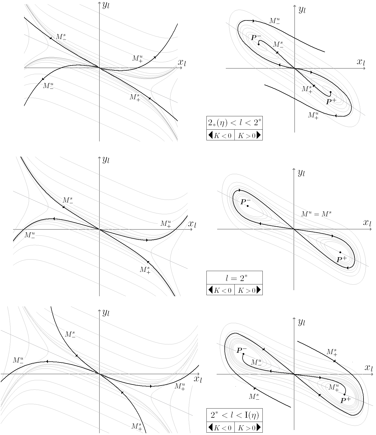
If and the origin is the unique critical point and both and are unbounded curves, see Figure 1.
In fact this analysis is easily extended to any autonomous system (S0) satisfying the following assumption, see [13] for details:
-
There is such that is -independent, is a constant, and is a function, which is positive increasing for and positive decreasing for , satisfying
This way we can consider e.g. (i.e. where ), or (i.e. ) where and are positive constants and and are larger than . So we can consider slightly more general functions .
Now we introduce a further notation which will be in force in the whole paper: we denote by the trajectory of (S) – or (S0) – which is in for .
The following remark underlines the relations between the behaviour of solutions of (S0) and of (Lr).
Remark 2.1.
This result can be easily proved using standard tools in invariant manifold theory, see e.g. [20, 23, 25]; we will prove it as a special case of a more general result, Lemma 2.5 below, in the non-autonomous context.
Assume now : the linearization of system (S) in the origin has real and distinct eigenvalues. Moreover the origin is a saddle iff or equivalently
| (2.3) |
where and have been defined in (1.3), (1.4). The eigenvalues are , where was defined in (1.5). Let us assume first that satisfies with , where the condition is replaced by . It is straightforward to check that, when the parameters are in the range (2.3), we have again a unique critical point in ; in particular if , we find , and . The point is unstable (either a node or a focus) if , a center if it is stable if (either a node or a focus). Again for we find that and are unbounded curves. See Figure 1. We refer to [25] for details.
We can again consider the stable manifold and the unstable manifold , in order to obtain estimates as in Remark 2.1, however the presence of the Hardy potential may forbid the existence of regular solutions. We will present such details in Section 2.3 in the non-autonomous case so to avoid repetitions.
2.2 Stable and unstable manifolds for non-autonomous systems.
In the previous subsection we have begun from the autonomous case for illustrative purposes. Now we turn to consider the -dependent case: the first step is the generalization of Remark 2.1. In this subsection we will make use of the following assumption for illustrative purposes (it will be removed from the next subsection):
- C
-
All the trajectories of (S) are continuable for any .
We have two different alternatives to introduce stable and unstable sets for non-autonomous systems, thus extending Remark 2.1 to a generic . The simplest one requires the strongest hypotheses, but gives more structure.
-
Assume H and that there is such that , for any , and
uniformly on compact sets, where the function is a non-trivial locally Lipschitz function satisfying and is a suitable positive constant.
-
Assume H and that there is such that , for any , and
uniformly on compact sets, where the function is a non-trivial locally Lipschitz function satisfying and is a suitable positive constant.
Assume and add to (S) the variable , to get
| (2.4) |
We have thus obtained an autonomous system and all its trajectories converge to the plane as ; so (2.4) is useful to investigate the asymptotic behavior in the past. The origin admits a -dimensional unstable manifold denoted by . From standard arguments of dynamical system theory, we see that the set is a -dimensional (immersed) manifold, for any , see e.g. [3, 24].
Similarly when holds we consider the following system to study the behavior of trajectories in the future, adding the new variable .
| (2.5) |
All its trajectories converge to the plane as . The origin admits a -dimensional stable manifold denoted by . Arguing as above, for any , is a -dimensional manifold.
Let us denote by the unstable manifold of the autonomous system (S) where and , and by the stable manifold of the autonomous system (S) where and . Then we have the following.
Remark 2.2.
Assume C and ; then approaches as . Assume ; then approaches as . More precisely, if (respectively ) intersects transversally a certain line in a point for (resp. for ), then there is a neighborhood of such that (resp. ) intersects in a point for any , and is continuous (in particular it is as smooth as ).
The proof of this Remark follows from standard facts in dynamical system theory. If we assume , it follows from [10, § 13], while if we allow to be a function satisfying H it follows from [12, Theorem 4.1] or [27, Theorem 2.16].
Following [29], which is based on [27], we can introduce stable and unstable leaves with assumptions weaker than and , see also the Appendix A.1 for a more detailed discussion of the topic.
-
Assume H and that there exists such that is continuous in uniformly for , whenever and for any in a compact set; further for any .
-
Assume H and that there exists such that is continuous in uniformly for , whenever and for any in a compact set; further for any .
Replacing by and by we can again construct -dimensional (immersed) manifolds , respectively , for any by characterizing them as follows:
| (2.6) |
Furthermore and in the origin are tangent respectively to the unstable and the stable space of the linearized system, see [27] and the Appendix for more details, in particular Remarks A.2 and A.3.
and have the smoothness property described above in Remark 2.2, but the first part of Remark 2.2 concerning their asymptotical behavior does not hold anymore (since and may be not defined). We stress that implies , and if the former holds then the manifolds constructed via and coincide; the specular result holds for which implies (this way we see that Remark 2.4 below holds for and if we assume and ). However observe that with and we allow also functions which are periodic in or which have logarithmic behavior. Further notice that when holds, the phase portrait is very different in the two cases and (see Figure 1), but in any case holds and guarantees the existence of the unstable manifold. A similar argument holds for and , too.
Since we want to understand the mutual position of these two objects we introduce the manifolds:
| (2.7) |
Notice that is omothetic to , and is omothetic to . Hence, they are -dimensional (immersed) manifolds for any .
Remark 2.3.
Observe that when holds for some , respectively holds for some , then holds for any , resp. holds for any .
The validity of the previous remark can be immediately verified: if we choose we have , where .
From now to the end of the subsection we assume for illustrative purposes; such a restriction is removed in the next subsection, which is focused on the novelties introduced by the Hardy term. We emphasize that, in any case, the result of this paper are new even for the original Laplace case, i.e. when . We also stress that the upper bound in the values of and due to , disappears when (since ).
Remark 2.4.
Assume , C, , , then and are tangent respectively to and to at the origin for any .
As in the -independent case, all regular solutions correspond to trajectories in , while fast decay solutions correspond to trajectories in . More precisely we have the following, see [23, 24].
Lemma 2.5.
Note that the manifold is split by the origin into two connected components, one which leaves the origin and enters the semi-plane (corresponding to regular solutions positive for small), denoted by , and the other which enters the semi-plane (corresponding to regular solutions negative for small), denoted by . Similarly is split by the origin into and , which leave the origin and enter respectively in and in (and correspond to fast decay solutions which are definitively positive and definitively negative respectively).
Now we turn to consider briefly singular and slow decay solutions, see e.g. [13].
Remark 2.6.
Assume and with , then (2.4) admits a critical point such that . This point admits an unstable manifold which is -dimensional if and -dimensional if . The trajectories contained in this manifold correspond to singular solutions of (Lr) such that . It is easy to check that if we have a unique singular solution, while if we have uncountably many singular solutions. Further, if , any trajectory of (S) bounded for converges either to or to or to the origin as .
Assume and with , then (2.5) admits a critical point such that . This point admits a stable manifold which is -dimensional if and -dimensional if . The trajectories contained in this manifold correspond to slow decay solutions of (Lr) such that . If we have a unique slow decay solution, while if we have uncountably many slow decay solutions. Further, if , any trajectory of (S) bounded for converges either to or to or to the origin as .
The proof follows from elementary arguments on the phase portrait, see e.g. [13, Lemma 2.9] for details.
2.3 Stable and unstable manifolds with Hardy potentials.
We go back to consider (Hr), and (S) where satisfies H. We list some results which explain similarities and differences with respect to Section 2.2. Their proofs rely on standard facts in invariant manifold theory for non-autonomous systems, and in particular on exponential dichotomy: they are postponed to the Appendix.
Remark 2.7.
Assume ; if regular solutions for (Hr) do not exist, due to the singularity of the equation for .
They are replaced by solutions which (may) exhibit a singular behavior as . More precisely,
for any there is a unique solution, of (Hr) such that
as .
Analogously assume ; then the behavior of fast decay solutions changes slightly. I.e., for any there is a unique
solution such that as (cf. Definition 1.1).
In particular, Lemma 2.5 continues to hold respectively for -solutions and -solutions.
Remark 2.8.
Assume and with and H (allow ). Then Remark 2.6, continues to hold almost with no differences: In particular -solutions are asymptotic to as , while -solutions are asymptotic to as . The only change is in the value of (which however can be computed explicitly).
We also observe that if , , H hold but , then there are no -solutions neither -solutions, so solutions of (Hr) which are defined in a neighbourhood of and are definitively positive for small are -solutions and the ones which are defined in a neighbourhood of and are definitively positive for large are -solutions.
Denote by . We recall that if is a constant matrix (e.g. when as for (Lr)), then the tangent spaces to and , say and , are independent from . This is not the case if . Let and be such that
| (2.8) |
Remark 2.9.
Assume , and allow ; then and , change smoothly with . Moreover as and as . Furthermore
Remark 2.10.
If , then , hence the -solution , with , is in fact singular, i.e. , and accordingly is negative and as . However if then , i.e. the -solution , with , is such that like a power as . Moreover it is monotone increasing for , since lies in for , and consequently the first branch of lies in for .
2.4 The lack of continuability
If C is removed the situation becomes more complicated.
Remark 2.11.
In this paper we are interested in functions which are negative for large and either small or large. In these cases equation (L) may admit solutions which are not globally defined, i.e. C is not fulfilled. So we adopt the following notation: we say that a solution , resp. a solution , is defined in a certain maximal interval with , resp. in with . We emphasize that as , and as , since the null solution is continuable for any .
We introduce the following definitions
| (2.9) |
Obviously the intervals and coincide with the whole if C is assumed, but they are bounded in the cases considered in this paper.
The lack of continuability is a relevant problem in order to apply dynamical system techniques and invariant manifold theory for non-autonomous systems. Let us denote by and the sets characterized as in (2.6). In the Appendix we will show that and may be disconnected. As usual, we can split these sets in their components and , which may be disconnected too.
For any fixed , let us denote by and respectively the connected component of and containing the origin, which are -dimensional manifolds, as we will see just below. We stress that there is no abuse of notation since, if C is assumed, and are -dimensional connected manifolds so they coincide with and respectively. Similarly, we can introduce the connected branches departing from the origin and without abuse of notation.
Lemma 2.12.
Assume and , then there are -dimensional immersed manifolds and with the following properties: they contain the origin, they are connected, and they are subsets of the sets and characterized as in (2.6).
Lemma 2.5 continues to hold with the following changes.
Lemma 2.13.
Assume and . Consider the trajectory of (S) with , and the corresponding trajectory of (S) with . Let be the corresponding solution of (Hr). Then .
Recall that , . Consider a -solution , then we can find such that and for any . Similarly consider a -solution , then we can find such that and for any .
The proofs of the previous lemmas are postponed to Appendix A.1.
Remark 2.14.
We stress that the tangents to and to in the origin coincide by construction with the tangents to and to . Hence, in Remark 2.4 we can remove assumption C.
2.5 Kelvin inversion and Fowler transformation
An important tool in the investigation of equations like (Hr) is a change of variables known as Kelvin inversion. Let us set
| (2.10) |
From a straightforward computation we see that satisfies (Hr) if and only if satisfies the following equation:
| (2.11) |
In particular, if is of type (1.1) then .
We stress that -solutions of (Hr) are driven by (2.10) into -solutions of (2.11), while -solutions of (Hr) are driven into -solutions of (2.11); we emphasize that , and . It is important to observe that generically if is subcritical (respectively supercritical) then is supercritical (resp. subcritical), see, e.g., [23, §2] for the analogous statement for (Lr).
We emphasize that Kelvin inversion (2.10) assumes a more clear form when it is combined with Fowler transformation (2.1). In fact, when we apply (2.1) to (2.11), by setting
| (2.12) |
we simply pass from system (S) to the following one:
| (2.13) |
We stress that (2.13) is obtained from (S) simply by changing the values of the parameters into , and evaluating the functions and in in spite of . We give the details of the computation for reader’s convenience. Let us set and introduce as in (2.10), then
Let us assume that satisfies with (respectively with ) then satisfies with (resp. with ), where
In particular we have and (resp. and ).
We emphasize that, if is independent, the condition means that (Hr) is subcritical (respectively and mean (Hr) supercritical and critical). Hence, it is clear that when we pass from (S) to (2.13), the unstable manifold is driven into the stable manifold and viceversa, and a subcritical system is driven into a supercritical system.
Moreover we emphasize that, in presence of a Hardy potential, we have e.g.
| (2.14) |
2.6 Statement of the results.
Let us introduce some further assumptions we will assume together with and .
-
There is , such that for any and any and for any .
-
There is , such that for any and any and for any .
We stress that is trivially satisfied if is as in (1.2a) and K holds, just setting . By symmetry, if is as in (1.2b) and K holds, follows.
We are now ready to state the main results, using the terminology introduced in Definition 1.1.
Theorem 2.15.
Consider (Hr) and assume with and , and . Then there are four positive strictly increasing sequences and such that is a positive , respectively is a negative .
For any , is a . In particular we have, and . Moreover is a positive for any , and for any , there is such that is a whenever . An analogous statement holds for where .
We recall that if satisfies with and , and , then obtained via (2.10) satisfies with and , and . Moreover -solutions are turned into -solutions and viceversa, and -solutions into -solutions, see Subsection 2.4. So, applying Kelvin inversion on Theorem 2.15, we obtain the following result.
Theorem 2.16.
Consider (Hr) and assume with and , and . Then there are four positive strictly increasing sequences and such that is a positive , while is a negative .
For any , is a . In particular we have, and .
Moreover is a positive for any , and for any , there is such that is a whenever . An analogous statement holds for where .
3 Proofs.
3.1 Preliminary lemmas.
For every solution of (S), we introduce polar coordinates
| (3.1) |
Taking into account (2.1),
we stress that if we switch between different values of , say and , we get
and , so we can drop
the subscript in .
In particular, the next remark easily follows from the fact that the flow on the -axis rotates clockwise, i.e.,
| (3.2) |
Let us denote by the integer part of .
Remark 3.1.
Consider the trajectory of a solution of (S);
then
is decreasing in .
Let us denote by and by , see (2.8); we assume w.l.o.g. that these functions are continuous, and and as and as respectively. Then we have the following.
Lemma 3.2.
Assume with and , then for any .
Proof.
From Remark 2.9 we have so that the conclusion easily follows from for sufficiently large, say . Moreover by we see that for any we have for any , where is a continuous increasing function such that , and is a continuous function such that is positive and finite. Therefore there is such that
| (3.3) |
Let us now consider the triangle having vertices , , , and denote by the edges opposite to , , , without endpoints.
Assume that we are in the hypotheses of Theorem 2.15.
From the manifolds exist for any . Moreover from we see that exists for any and its tangent at the origin is where as , see Remark 2.9.
Let and be smooth parameterizations respectively of and such that and . We assume w.l.o.g. that the functions and are continuous in both the variables.
The following result establishes a correspondence between trajectories of (S) and solutions of (Hr).
Lemma 3.3.
The proof is postponed to Appendix A.2, however see [13, Lemma 2.10] for the simpler case where and C is assumed.
Lemma 3.3 permits us to introduce an additional parametrization on our manifolds depending on the parameters and .
Remark 3.4.
For every , we can parametrize directly with and with . In this way we can introduce the new parametrizations and , which are continuous in both the variables; here have been defined in (2.9). However in this case cannot be extended continuously to and cannot be extended to , since as and as , for any and .
We underline that, in general, we do not have or . E.g., by Remark 2.11, once fixed , if for a certain then . An analogous statement holds for and .
Remark 3.5.
Assumption guarantees both forward and backward continuability of the trajectories of (S) for . Therefore , and for any .
Using (2.7) we can define for the continuous parameterizations . It is straightforward to check that the property explained in Lemma 3.3 holds for , too.
We need to consider also the following parametrizations in polar coordinates of the manifolds:
| (3.6) |
| (3.7) |
We recall that the angular coordinate of the parametrizations does not depend on the choice of as stated in Lemma 2.5.
Let and consider the trajectory of (S). Note that approaches as , see (2.8). Using the polar coordinates introduced in (3.1), let us set
| (3.8) |
where we can assume that the angular coordinate satisfies . Similarly, if we consider with the trajectory , then approaches as , and we can assume . However, if for a certain , we must choose one of the two conditions, the other will be satisfied up to a multiple of .
3.2 Proof of the main theorems.
In this section we provide the proof of Theorem 2.15. The proof is based on some geometrical observations on the phase portrait. Then Theorem 2.16 follows from Kelvin inversion.
We recall that the manifolds are sets of initial conditions converging to the origin and a priori they are not graphs of solutions unless the system is autonomous. However, for system (S) the number of rotations around the origin performed by from the origin until a point , equals the number of rotations performed by the trajectory for , with reversed sign.
More precisely we have the following property, the proof is adapted from [13, Propositions 3.5, 3.8] (we refer also to [3, 24, 30] for more details) and it is postponed to Appendix A.2.
Lemma 3.6.
We wish to underline that a similar statement can be obtained for the unstable manifold too. Moreover, notice that Lemma 3.6 is independent from the parametrization of the stable manifold, so we can use the one defined in (3.7).
Lemma 3.7.
Assume with , and , then and are spirals rotating indefinitely counterclockwise around the origin for any ; therefore , and for any .
Proof.
We prove the Lemma just for ; the case of can be obtained analogously. The Lemma is known if the system is autonomous, so we have it trivially for . In fact the manifold coincides with the stable manifold of the autonomous system (S) where . We recall that from we get continuability of the solutions for any . From Remark 2.2, we see that for any integer there is such that crosses transversally the coordinate axes, and performs at least complete rotations counterclockwise, for any . In particular, using (3.7), there exists such that . Call which belongs to the positive -semiaxis. In particular performs more than complete rotations.
Let be the angular coordinate of , see (3.8), then from Lemma 3.6 we see that . By (3.2) and Remark 3.1, we have, for any , as long as exists, therefore at least for . Then using again Lemma 3.6 and Lemma 3.2, we see that
thus obtaining that draws more than rotations for every . We have thus proved the Lemma, since is arbitrarily large. ∎
Lemma 3.8.
Assume and ; then , and
for every and for any .
Proof.
As usual, we give the proof for , the other follows similarly. Let
Notice that is increasing, and by , for any fixed . Let , and set , .
This proof is analogous to the one of Lemma 3.2 and relies on Lemma A.6. We construct the triangle with vertices , , , and with edges , , opposite to the vertices , , respectively.
Let at a certain time , then
| (3.10) |
From we see that if at a certain time , then
| (3.11) |
So from (3.10), (3.11) the flow of (S) on , points towards the interior of , for any .
Assume first so that on we have . The flow on points towards the exterior of ; hence we can apply Lemma A.6, and we find a connected subset containing and a point in , for any and any . Such a procedure can be repeated for arbitrarily large, thus concluding the proof of the lemma.
Now assume . From Remark 2.3 we see that holds for too, so we can construct and . Fix as above and consider the flow of (S) for . We construct again the triangle and we observe that (3.10) and (3.11) continue to hold, and the flow of (S) on points outwards. So we conclude via Lemma A.6 as above the existence of a subset of such that and . So we prove the Lemma for for the arbitrariness of . Then, recalling that and are omothetic we conclude. ∎
The following lemma investigates the presence of intersections between the unstable manifold and the manifolds which are omothetic to the stable manifold . A similar reasoning was adopted already in [3, 13, 25, 30].
Lemma 3.9.
Assume the hypotheses of Theorem 2.15. Then intersects in a sequence of points , for any , where is defined in . Moreover, we can assume that if is even, while if is odd.
Proof.
Fix . From Lemma 3.7 we know that and are two spirals rotating counterclockwise around the origin, and each of them is cut infinitely many times by (see Figure 2): at least once at each rotation respectively at the point and , by the property shown in Lemma 3.8.
We develop this argument in polar coordinates too, for clarity and for later purposes. Using also Lemma 3.2 we see that
Consider the following curves in the stripe :
| (3.12) |
for . Let us introduce, for every ,
| (3.13) |
(except ) and notice that holds by construction, all having the same sign. In fact, roughly speaking, we have denoted with “” the intersections of the stable manifold (the first at any lap) with the positive -semiaxis and with “” the ones with the negative; moreover even subscripts correspond to the intersections of , respectively odd subscripts to the ones of (cf. Figure 2a).
Let be the open region delimited by and the lines and (see again Figure 2a). Similarly let be the open region delimited by and the lines and . It is easy to check (see e.g. the proof of Lemma 3.9 in [13] for details) that, for any , the curve is in for small and outside for large. So it intersects the graph of : these intersections corresponds to distinct points . We are interested in the first intersections, in the sense of the parameter , so let us set
| (3.14) | ||||
for any . We denote by the unique value in such that , and we set , and , the corresponding switched polar coordinates (see Figure 2a). Moreover, notice that by construction holds, all having the same sign. ∎

Remark 3.10.
A similar result can be obtained for the unstable manifold (cf. Figure 2a): the curve must exit from , so intersects the stable manifold in the distinct points with switched polar coordinates . In particular if is even, while if is odd. Moreover, we can identify the corresponding sequences , , with and , such that . Let us set ; by construction we find , all having the same sign. We stress that the sequences in the statement of Theorem 2.15 can be now introduced as , , and , and : they are strictly increasing by construction.
By construction, is a homoclinic trajectory of (S), and the corresponding solution of (Hr) is a solution. We introduce the following notation: let be a point in , and ; we denote by the switched polar coordinates of , such that (so that it is uniquely defined). With a little abuse of notation we denote by the switched polar coordinates of , where , and we observe that the angular coordinate is the same as in , while the radial coordinate is multiplied by .
Lemma 3.11.
Assume the hypotheses of Theorem 2.15. Then, is . In particular, is a positive solution.
Proof.
When we consider (Lr) we can simply repeat the proof of [13, Lemma 3.11] with no changes. When we deal with (Hr) we need to adapt slightly the argument: we sketch the proof for reader’s convenience.
If is even we have , while if is odd we have , see also Lemma 3.6. Therefore performs the angle around the origin when , and it performs the angle for every when . Summing up, performs the angle . Since we see that crosses the axis exactly times and so changes sign exactly times. ∎
Remark 3.12.
The solution of (Hr) is a , and it is definitively positive for even and definitively negative for odd. However, a priori, we may find some , for any such that is a (cf. Figure 2b). In fact it may happen e.g. that intersects in, say, three points: at , thus corresponding to three distinct points . In this case we have three positive : , , , see [13, Section 3] for a more detailed discussion of this point.
Remark 3.13.
We emphasize that and are well defined for any , , whenever , cf . Next if intersects in , then intersects in a point corresponding to the same solution , for any .
Following the ideas of [13, Section 3], let us now turn to consider the solution where for any . Fix , we need to define several subsets of the stripe :
| (3.15) |
for any . We denote by the open set enclosed by , and the line , which is bounded for any and any . Further set and, for ,
Observe that if has a unique intersection with then (in general we have ). We set (cf. Figure 2b)
| (3.16) |
Define and, for any , denote by the open bounded set enclosed by , , and the line (observe that ). Note that these sets have the following property.
Remark 3.14.
If belongs to , , , , for some then belongs respectively to , , , for any .
Proof.
We just sketch the proof which is strongly inspired by [13, Section 3] and in particular [13, Lemma 3.14]. The claim concerning , follows from construction. Then note that if then too, and the same property holds for . It follows that if then cannot cross and , hence it is forced to stay in for any . The claim concerning is analogous. ∎
Now we turn to consider solutions.
Lemma 3.15.
Proof.
From Lemma 3.8, we know that . Moreover is a path connecting the point to , where . From Lemma 3.7 we see that is a path connecting a point to , where as , and .
Let be the switched polar coordinates of and the switched polar coordinates of the trajectory corresponding to the same solution of (Hr), so that .
Let us denote by , , and similarly for , , . By construction , , , iff , , .
Denote by the switched polar coordinates for , and set
We define as the unbounded open stripe between and . Observe further that corresponds to the unbounded open subset between and for (S), the one containing if is even and the one the one containing if is odd.
Note that as approaches a bounded open subset of , say containing the switched polar coordinates either of if is even or of if is odd; similarly approaches a subset of as . Moreover note that (or ) is the unique attracting subset of . Let be switched polar coordinates for .
Then observe that if (respectively ) then (resp. ) and converges to (resp. ) as . Moreover if (respectively ) then as , and again (resp. ), and converges to (resp. ) as ; hence the corresponding solution of (Hr) is a (resp. a ) which is definitively positive (resp. negative). ∎
4 Some further examples.
In this section we briefly present other types of nonlinearities to which our theorems apply. Let us begin by noticing that when is as in (1.2a), arguing as in Section 2.1, we can choose and as in Corollary 1.2, and we get
where , and and go to as . In fact we can also consider logarithmic growth, e.g.
| (4.1) |
where , , . In this case assumption does not hold but holds for any , see (1.7). So if K holds with the first in (1.6) replaced by (4.1) we can apply Corollary 1.2. Similarly if is as in (1.2b) and K holds with the second in (1.6) replaced by , , then holds for any , so we can apply Corollary 1.3.
Introduce
| (4.2) |
for a certain integer , where , , are continuous functions which are bounded and uniformly far from zero for small and large, negative near zero, changes sign at and then they are positive. We assume
thus having
Moreover it is possible to assume that some of the are identically zero for either or . We do to not enter in details for major clarity. Assume now
| (4.3) |
Setting and remembering that, for , one has , where , a computation gives the validity of if . The first condition of holds simply setting , while we have to assume
| (4.4) |
in order to fulfill the second one. Roughly speaking, the term with the greatest power is the first to change sign.
Assumption holds setting . Hence, Theorem 2.15 applies if is as in (4.3) with and such that (4.4) holds.
Arguing as above we can find the corresponding specular conditions in order to permit the application of Theorem 2.16. Assume with as in (4.2) assuming now . Setting we have , then set and assume (4.4) so that is given. The validity of is given setting , asking .
The functions previously considered consist of sum of possibly different polynomial terms. However, our results permit us to consider also more general nonlinearities, which however have a leading term in their expansion for small and large which is polynomial, e.g.
assuming , and , . In such a case, a straightforward computation gives that holds requiring and holds setting .
Further notice that our results are robust. I.e., we have the following.
Remark 4.1.
Assume H and consider (for simplicity) the functions , satisfying the assumption of Corollary 1.2, and 1.3 respectively.
Let be such that ; suppose that there is such that for and for , and that uniformly for .
The assumptions on Hardy potentials are more clear so we just emphasize the following interesting example satisfying H:
Appendix A Appendix
A.1 On the lack of continuability
In this appendix we first review briefly some well known facts concerning exponential dichotomy, see, e.g., [12]. Then we develop the construction of stable and unstable manifolds for non-autonomous systems, i.e. and , when continuability of the trajectories of (S) is ensured, i.e. when hypothesis C holds. Then we extend our discussion to the case where C does not hold.
Denote by the linearization of the right hand side of (S) in the origin, and by . Assume either or : note that has as eigenvalues where and . By H, can be seen as an perturbation of , therefore it admits exponential dichotomy in negative semi-lines . More precisely let be the fundamental matrix of
| (A.1) |
i.e. the matrix solution of (A.1) such that , where denotes the identity matrix. Then, for any there is a constant , exponents and a projection such that
| (A.2) |
see, e.g., [12, Section 4]. Moreover the optimal choice for is for , see [8, Appendix]. Let us denote by , and by the -dimensional kernel of ; then is the unstable space for (A.1). I.e let , and denote by the solution of (A.1) such that ; then is bounded for iff , cf. [12, Section 4]. Since is -dimensional we see that there is such that as . Also note that by construction is a line, and iff .
Now assume and consider (S) where : we consider this problem as a nonlinear perturbation of (A.1). Thus, setting , we get the following, see [27, Theorem 2.25].
Lemma A.1.
Assume ; then for any we can find such that the set
| (A.3) |
is a graph on for any . Moreover is the tangent space to in the origin.
We sketch the proof for completeness. Assume and suppose first that,
for some and for any . Then, using a variation of constants formula, see e.g. [11, Section 3.3] or [27, Theorem 2.25], we prove that the set, cf. (2.6),
| (A.4) |
is a graph on (globally), for any . Then the proof follows from a truncation argument.
Using the flow of (S) we get the following.
Lemma A.2.
Assume and C. Then the set characterized as in (A.4) is a -dimensional immersed submanifold having as tangent space in the origin.
Proof.
Remark A.3.
We stress that (and constructed below) may be not a usual submanifold in the origin: i.e it may be shaped as in the critical autonomous case, see e.g. Figure 1. However it always contains (respectively ) which is tangent to (resp. ).
Now we drop the assumption C and we prove Lemma 2.12.
Proof of Lemma 2.12. Fix ; for every we can introduce
Then if . It is easy to verify that is lower semicontinuous, i.e. the sets are closed. In fact for every and every we can find neighbourhoods of and of such that for every we have , thus giving for every . Therefore if , then .
Then, we consider
| (A.5) |
Notice that and that is increasing by construction. The lower semicontinuity gives us that either one has or the infimum is in fact a minimum, being bounded and . Moreover the subset containing the points which explode to infinity before a fixed time ,
is a closed subset. Conversely is a relatively open subset of .
If , then , so that is diffeomorph to , and it is a -dimensional manifold with border. In fact it is easy to check that the map is well defined in an open neighborhood of .
t

We assume first for illustrative purpose that, for any the function is strictly decreasing in : this is the case, e.g., if (S) is autonomous. This assumption will be removed later on.
If we set we have where is the endpoint of , while if the sets , which contains , and are connected. In both the cases, the map is well defined on , and the set is diffeomorph to . In fact there is an open neighborhood of which is mapped by the inverse diffeomorphism into an open neighborhood of . So is a -dimensional manifold without border, see Figure 3.
Now let us repeat the discussion replacing by . It is easy to check that , and if , then , and it is unbounded. Furthermore by construction
| (A.6) |
if . Therefore the set
is characterized by the property defined in (A.6).


If we remove the simplifying assumption that is decreasing with respect to , we can repeat the previous discussion with the following changes. The open set can be disconnected, so its image may be disconnected too, see Figure 4. However has a connected component containing the origin, say , whose image is the connected component of containing the origin. Observe that is a connected one dimensional manifold, so this property is inherited by too.
When , the map is well defined in and the set may disconnect , see Figure 5. Repeating the previous arguments we see that the image is unbounded and may have many components. However, has a connected component containing the origin, say and we can consider the image which is a -dimensional connected manifold and it is unbounded.
Again, cf. Figure 4, if we switch from to we see that , and if , then
for any . Hence, we can define for every the set
which is a -dimensional connected manifold containing the origin in its border, and it is unbounded. Reasoning in the same way we see that if then
therefore we can define
Notice that may not be a manifold (it may break infinitely many times), since may be disconnected. However by construction may be still characterized as in (A.6); moreover is the connected component of containing the origin in its border, and it is, as shown above, a -dimensional connected manifold.
The construction of and of is completely analogous and it is omitted. This concludes the part of the proof of Lemma 2.12 concerning the unstable manifolds. The construction of the stable leaves is very similar and we just sketch it.
With a specular argument we assume , so that has as eigenvalues, where and . So, let be the fundamental matrix of (A.1), where is replaced by . Then, for any there is a constant , and a projection such that
| (A.7) |
see again [12, Section 4], and [8, Appendix]. Denote by , and by the -dimensional range of . Then the solution of (A.1), with replacing , is bounded for iff . Moreover as for a suitable . This way we are able to construct a local manifold and to reprove a result analogous to Lemma A.1. Then, assuming temporarily C and reasoning as in Lemma A.2, we see that is a -dimensional submanifold for any ; moreover if . Hence, assuming C and , we obtain that the set
| (A.8) |
is a -dimensional immersed manifold having as tangent space in the origin.
Then we remove assumption C and, arguing as above, we see that may be disconnected, but its connected component containing the origin, denoted by , is again a -dimensional manifold. Then repeating the previous discussion we conclude the proof of Lemma 2.12. The part of the proof concerning Lemmas 2.5 and 2.13 is given below. ∎
Now we proceed with the proof of Lemma 2.13, which includes Lemma 2.5 as a particular case. The proof is adapted from [13, Lemma 2.10] where it is developed assuming C and .
Proof of Lemma 2.13
Assume and ; recalling that
, we find
.
Therefore in particular .
Assume first C for simplicity. From roughness of exponential dichotomy, cf [12, Chapter 4] and [27, Theorem 2.16], we see that, if , then there is such that . Assume for definiteness; then for the corresponding solution of (Hr) we get
| (A.9) |
Assume now . Then, if , we find that is uniformly positive as , and if there is a sequence such that is uniformly positive: in both the cases the corresponding solution of (Hr) is not a -solution since as . Further we easily see that .
Arguing similarly, if then there exists such that : hence the corresponding solution of (Lr) satisfies
| (A.10) |
So we can easily conclude as above.
Hence, if we assume either or , we can construct the unstable manifold for any ; similarly if either or hold, we can construct the stable manifold for any . Moreover Remark 2.2 still holds and we can construct and via (2.7) too.
Now we drop assumption C. In this case, due to the presence of non-continuable trajectories, we need to distinguish between and , and similarly for the other manifolds. In fact iff . Further for any we can find such that for any . So we can repeat the previous argument and we see that the corresponding solution of (Hr) is a -solution. A similar argument holds for the stable manifold.
So for any we find that iff iff is a -solution with , see (2.9). Similarly iff if is a -solution with . ∎
A.2 Proof of Lemmas 3.3 and 3.6
We prove now Lemma 3.3: such a result has been obtained in presence of continuability of the solutions and for in [13, Lemma 2.10].
Proof of Lemma 3.3. We will prove only the first part of the statement, the second follows similarly. Consider the parametrization . Assume first C. Observe that, starting from , we can construct a parametrization of for any , by setting . In fact, the function is continuous in both the variables, and the map is injective in . According to this parametrization, coincides with and corresponds to the given solution for any .
Fix and let be the constant defined in Lemma A.1; we can find and such that , whenever and .
We now show that is strictly increasing. Once proved this claim for this particular parametrization we have it for any parametrization of as in the assumption of Lemma 3.3, due to the monotonicity of the change of variables . Using Lemma A.1 we see that we can choose , so that for any and for . Hence is a graph on , for any , see Lemma A.1. In particular for . We claim that is a graph on a segment of the axis, for any . In fact when the claim is obvious since is contained in the axis. If , since is not orthogonal to the axis, possibly choosing a smaller we can again assume that is a graph on the axis too, so the claim is true.
Assume for contradiction that , then there is such that is positive for any and it is zero for . In particular is not a graph on the axis, so we have found a contradiction. Hence , and the Lemma is concluded if C holds. Notice that we can redefine the parametrization and use directly instead of as parameter, so, with a little abuse of notation we find the parametrization of which is continuous (and smooth) in both the variables for any .
Now we drop C. Fix , and correspondingly as in (2.9), so that, for any ), is continuable for any . Using the previous discussion and a truncation argument, for any , we can define the map for ; so we get a parametrization of a connected branch of , say . Since for any point we have that exists for any , arguing as above, we find that is a parametrization of a connected branch of , denoted again by , for any .
Now let and notice that the function defined in (2.9) is decreasing in . If , reasoning as above, we find that gives again a parametrization of a connected branch of , for . If then for is unbounded and it is itself a parametrization of the whole manifold . Assume , this way we obtain a map which is continuous in both the variables for
Further is injective for . For the arbitrariness of we can let . Then from the arbitrariness of we define in the whole , it is continuous in both the variables and it gives a bijective parametrization of for any . ∎
Now we prove Lemma 3.6: the argument is a modification of [13, Propositions 3.5, 3.8]. In fact, in this setting, we need to take into account the fact that and change with (due to the presence of Hardy potentials), while in [13] there was not this difficulty. In particular we need to ask for and to profit of Lemma 3.2.
Proof of Lemma 3.6. We introduce some definitions borrowed from [3, 24]. Following [3, 24, 30], given a curve , we define its rotation number by setting
| (A.11) |
where denotes the integer part, and As pointed out in [24], we can extend this definition to a curve defined in a semi-open interval if exists (even if it is infinite).
Our argument will be rather sketchy since we just adapt [13, 24]. Let , for , be curves in which do not intersect each other, and let be a smooth monotone function such as as in (2.4), or as in (2.5) or as in [3]. Then are curves in . Following [3], we call linking number of in the number , i.e. the number of complete rotations of a curve around the other. Such a quantity is invariant for homotopies in which preserve the endpoints and .
We want to establish an homotopy between two curves so that linking number and rotation number are equal. Let us fix and . Since converges to the origin as and for , for every we can find such that and for .
Then we set , where ,
and we consider the trajectory of (2.4)
for .
We shrink further so that the sets defined in Lemma A.1
are graphs on for any , and we denote by
the unique point in .
Let be such that and
.
We consider the curves for , the curve
for and the curve obtained following the graph of and then the graph of .
An homotopy between and
is obtained by projecting
on following the -dimensional manifold : we sketch the construction,
see [24, Lemma 4.3] for more details.
For any we construct the function obtained following for , then for and finally for i.e.
Note that all the curves have the same endpoints and are homotopic; moreover is and is . So the linking number of and is .
A.3 On the Wazewski’s principle
We conclude the appendix with a result, inspired by Wazewski’s principle, which allows to locate the unstable and the stable manifolds. Consider
| (A.13) |
where , , continuous, and assume that the origin is a critical point for (A.13).
Let be a closed set diffeomorphic to a full triangle. We call the vertices , and , and , , the edges (without endpoints) which are opposite to the respective vertex. Let denote a further set diffeomorphic to a full triangle having as vertex and with edges and ; it follows that . We begin from a result requiring very weak regularity properties.
Lemma A.4.
Assume that local uniqueness for the solutions of (A.13) is ensured for any trajectory starting from .
Suppose that the flow on points towards the interior of , and on points towards the exterior of for any . Assume further that the flow on points towards the interior of for any . Finally suppose that if a solution of (A.13) satisfies for any , then .
Then there is a compact connected set such that , , with the following property:
Proof.
Obviously the same idea can be applied to construct stable sets.
Lemma A.5.
Assume that local uniqueness for the solutions of (A.13) is ensured for any trajectory starting from .
Suppose that the flow on points towards the exterior of , and on points towards the interior of for any . Assume further that the flow on points towards the exterior of for any . Finally suppose that if a solution of (A.13) satisfies for any , then .
Then there is a compact connected set such that , , with the following property:
If we are in the position to apply invariant manifold theory for non-autonomous systems, clearly we find that these sets are manifolds. So we get the following.
Lemma A.6.
Assume that we are in the hypotheses of Lemma A.4, respectively of Lemma A.5. Assume further that is and it is continuous in uniformly with respect to . Suppose that the linearized system admits exponential dichotomy, i.e. there are projections and of rank such that (A.2) and (A.7) hold, so that admits unstable and stable manifolds and for any . Then the set constructed in Lemma A.4, resp. the set constructed in Lemma A.5, is a connected -dimensional manifold.
References
- [1] S. Bae, On positive entire solutions of indefinite semilinear elliptic equations, J. Differential Equations 247, no. 5, 1616-1635 (2009).
- [2] S. Bae, Classification of positive solutions of semilinear elliptic equations with Hardy term, Discrete Contin. Dyn. Syst. Supplement, 31-39 (2013).
- [3] R. Bamon, M. Del Pino and I. Flores, Ground states of semilinear elliptic equations: a geometric approach, Ann. Inst. Henry Poincaré 17, 551-581 (2000).
- [4] F. Battelli and R. Johnson, On positive solutions of the scalar curvature equation when the curvature has variable sign, Nonlinear Anal. 47, 1029-1037 (2001).
- [5] G. Bianchi, Non-existence of positive solutions to semilinear elliptic equations on or through the method of moving planes, Comm. Partial Differential Equations 22, 1671-1690 (1997).
- [6] D. Bonheure, J. Gomes, P. Habets, Multiple positive solutions of superlinear elliptic problems with sign-changing weight J. Differential Equations 214, no. 1, 36-64, (2005,.
- [7] P. Cac, A. Fink and J. Gatica, Nonnegative solutions of the radial laplacian with nonlinearity that changes sign Proc. Amer. Math. Soc. 123, 1393-1398 (1995).
- [8] A. Calamai and M. Franca, Mel’nikov methods and homoclinic orbits in discontinuous systems, J. Dyn. Differential Equations 25, no. 3, 733-764 (2013).
- [9] F. C. Cîrstea: A complete classification of the isolated singularities for nonlinear elliptic equations with inverse square potentials, Mem. Amer. Math. Soc. 227, no. 1068, (2014).
- [10] E. Coddington and N. Levinson: Theory of Ordinary Differential Equations , Mc Graw Hill, New York, (1955).
- [11] W.A. Coppel: Stability and asymtotic behavior of differential equations, Heath Mathematical Monograph, (1965).
- [12] W.A. Coppel: Dichotomies in stability theory, Lecture Notes in Mathematics 377, Springer, Berlin, (1978).
- [13] F. Dalbono and M. Franca, Nodal solutions for supercritical Laplace equations, Comm. in Math. Phys. http://dx.doi.org/10.1007/s00220-015-2546-y
- [14] Y.-B. Deng, Y. Li, Y. Liu, On the stability of the positive radial steady states for a semilinear Cauchy problem, Nonlinear Anal. 54, 291-318 (2003).
- [15] Z. Dosla, M. Marini and S. Matucci, Positive solutions of nonlocal continuous second order BVP’s, Dynam. Systems Appl. 23, no. 2-3, 431-446 (2014).
- [16] V. Felli, E. Marchini, S. Terracini, On the behavior of solutions to Schrödinger equations with dipole type potentials near the singularity, Discrete Contin. Dyn. Syst. 21, no. 1, 91-119 (2008).
- [17] V. Felli, E. Marchini and S. Terracini, Fountain-like solutions for nonlinear elliptic equations with critical growth and Hardy potential, Commun. Contemp. Math. 7, no. 6, 867-904 (2005).
- [18] A. Ferrero and F. Gazzola, Existence of solutions for singular critical growth semilinear elliptic equations, J. Differential Equations 177, 494-522 (2001).
- [19] R.H. Fowler, Further studies of Emden’s and similar differential equations, Quart. J. Math. 2, 259-288 (1931).
- [20] M. Franca, Some results on the m-Laplace equations with two growth terms; J. Dynamics Differential Equations, 17, 391-425 (2005). http://dx.doi.org/10.1007/s10884-005-4572-5
- [21] M. Franca, Non-Autonomous Quasilinear Elliptic Equations and Wazewski’s principle, Topol. Methods Nonlinear Anal. 23, 213-235 (2004).
- [22] M. Franca, Radial ground states and singular ground states for a spatial dependent -Laplace equation, J. Differential Equations 248, 2629-2656 (2010).
- [23] M. Franca, Positive solutions for semilinear elliptic equations with mixed non-linearities: 2 simple models exhibiting several bifurcations, J. Dynam. Differential Equations 23, 573-611 (2011).
- [24] M. Franca, Positive solutions of semilinear elliptic equations: a dynamical approach, Differential Integral Equations 26, 505-554 (2013).
- [25] M. Franca and A. Sfecci, On a diffusion model with absorption and production, arXiv:1606.02196
- [26] B. Gidas, W.M. Ni and L. Nirenberg, Symmetry of positive solutions of nonlinear elliptic equations in , Adv. Math. Suppl. Studies 7A, 369-402 (1981).
- [27] R. Johnson, Concerning a theorem of Sell, J. Differential Equations 30, 324-339 (1978).
- [28] R. Johnson, X.B. Pan and Y.F. Yi, Singular ground states of semilinear elliptic equations via invariant manifold theory, Nonlinear Anal. 20, no. 11, 1279-1302 (1993).
- [29] R. Johnson, X.B. Pan and Y.F. Yi, Positive solutions of super-critical elliptic equations and asymptotics Comm. Partial Differential Equations 18, no. 5-6, 977-1019 (1993).
- [30] C. Jones and T. Kpper, On the infinitely many solutions of a semilinear elliptic equation, SIAM J. Math. Anal. 17, 803-835 (1986).
- [31] Y. Li and W. Ni, Radial symmetry of positive solutions of nonlinear elliptic equations in Comm. Partial Differential Equations 18, no. 5-6, 1043-1054 (1993).
- [32] M. Marini and S. Matucci, A boundary value problem on the half-line for superlinear differential equations with changing sign weight, Rend. Istit. Mat. Univ. Trieste 44, 117-132 (2012).
- [33] S. Matucci, A new approach for solving nonlinear BVP’s on the half-line for second order equations and applications Math. Bohem. 140, no. 2, 153-169 (2015).
- [34] J. D. Murray: Mathematical biology. II. Spatial models and biomedical applications. Third edition, Interdiscip. Appl. Math. 18, Springer, New York, (2003).
- [35] Ni W.M. and Serrin J., Nonexistence theorems for quasilinear partial differential equations, Rend. Circolo Mat. Palermo (Centenary supplement), Series II 8, 171-185 (1985).
- [36] D. Papini and F. Zanolin, Periodic points and chaotic-like dynamics of planar maps associated to nonlinear Hill’s equations with indefinite weight., Georgian Math J. 9, 339-366 (2002).
- [37] S. I. Pohozaev, Eigenfunctions of the equations , Soviet Math. Dokl 5, 1408-1411 (1965).
- [38] S. Terracini, On positive entire solutions to a class of equations with a singular coefficient and critical exponent, Adv. Differential Equations 1, 241-264 (1996).
- [39] X. Wang, On the Cauchy problem for reaction-diffusion equations, Trans. Am. Soc. 337, no. 2, 549-590 (1993).
- [40] E. Yanagida, Structure of radial solutions to in , SIAM J. Math. Anal. 27, no. 3, 997-1014 (1996)