Magnetic field effects on the static quark potential at zero and finite temperature
Abstract
We investigate the static potential at zero and finite temperature in the presence of a constant and uniform external magnetic field , for several values of the lattice spacing and for different orientations with respect to . As a byproduct, we provide continuum limit extrapolated results for the string tension, the Coulomb coupling and the Sommer parameter at and . We confirm the presence in the continuum of a -induced anisotropy, regarding essentially the string tension, for which it is of the order of 15% at and would suggest, if extrapolated to larger fields, a vanishing string tension along the magnetic field for GeV2. The angular dependence for GeV2 can be nicely parametrized by the first allowed term in an angular Fourier expansion, corresponding to a quadrupole deformation. Finally, for , the main effect of the magnetic field is a general suppression of the string tension, leading to a precocious loss of the confining properties: this happens even before the appearance of inverse magnetic catalysis in the chiral condensate, supporting the idea that the influence of the magnetic field on the confining properties is the leading effect originating the decrease of as a function of .
pacs
12.38.Aw,11.15.Ha,12.38.Gc,12.38.MhI Introduction
In the Standard Model, the strong and the electroweak sectors are connected by quarks, which are subject to both type of interactions. In general, electroweak interactions are expected to induce relatively small corrections to strong interaction dynamics, however this may be not true in the presence of very strong electromagnetic backgrounds, with field values comparable to the QCD scale. This is a situation which is relevant to many contexts, ranging from non-central heavy ion collisions [1, 2, 3, 4, 5, 6] and the cosmological electroweak phase transition [7, 8], with magnetic fields reaching or exceeding Tesla ( GeV2), to magnetars [9], where magnetic fields are expected to be of the order of Tesla on the surface but could be significantly larger in the inner cores.
How strong interactions get modified by such large magnetic fields has been the subject of many recent theoretical studies (see, e.g., Refs. [10, 11] for reviews), with lattice simulations representing a viable and effective tool to explore the issue starting from the first principles of QCD. One important feature is that gluon fields, even if not directly coupled to electromagnetic fields, undergo significant modifications, through effective QED-QCD interactions induced by quark loops, as can be seen both by lattice simulations [12, 13, 14, 15, 16, 17, 18, 19, 20, 21, 22, 23, 24, 25, 26, 27, 28] and by analytical studies using several approaches, which range from perturbation theory to effective field theories, from NJL models to functional renormalization group techniques [29, 30, 31, 32, 33, 34, 35, 36, 37, 38, 39, 40, 41, 42, 43, 44, 45, 46, 47, 48, 49, 50]. A striking consequence of the QED-QCD coupling is the distortion of the zero temperature static quark-antiquark potential. Results reported in Ref. [21] showed the emergence of anisotropies both in the linear part (string tension) and in the Coulomb part of the potential. This behaviour is consistent with the results of some of the existing model computations [51, 52, 53, 54, 55] and may have relevant phenomenological consequences, especially for the spectrum of heavy quark bound states [56, 57, 58, 59, 60, 61, 62, 63, 64, 65].
The purpose of this study is to move one step forward in our comprehension of magnetic-induced effects on non-perturbative QCD dynamics. First of all, we present a refinement of our zero temperature data following three different directions:
- •
a complete analysis of the angular dependence of the potential (in Ref. [21] only quark-antiquark separations parallel and orthogonal to the magnetic field were analyzed). This is important to allow for a realistic modelling of the quark-antiquark potentials to be used in the computation of the spectrum of heavy quarkonia;
- •
the inclusion of new simulations on finer lattices will permit us to extrapolate results reported in Ref. [21] to the continuum limit;
- •
the investigation in the regime of fields significantly larger than those used in Ref. [21], in order to inquire whether new unexpected phenomena may take place in the QCD vacuum under the influence of extremely strong background fields.
As a byproduct of this investigation, we will provide a continuum extrapolation of the static quark-antiquark potential with physical quark masses also for the standard case of vanishing magnetic field.
In the second part of our study, we investigate how the effect of the magnetic field on the static potential gets modified by the temperature, a step which is important for a full comprehension of the properties of the thermal medium in the presence of magnetic backgrounds. In this case the static potential (more correctly the free energy) is extracted from Polyakov loop correlators in place of Wilson loop expectation values used at . For temperatures below the pseudo-critical temperature (at which chiral symmetry gets restored and quark and gluon degrees of freedom deconfine), one still expects that heavy quark-antiquark interactions can be described in terms of a confining potential, with a string tension which goes to zero as is approached. Two main questions will be addressed by our study in this regime: i) does the anisotropy survive also in the finite temperature case? ii) does the magnetic field enhance the suppression of the string tension, meaning that a phenomenon similar to inverse magnetic catalysis [17], observed for chiral symmetry, takes place also for the confining properties of the medium?
The paper is organized as follows. In Section II we illustrate the setup of our numerical simulations and the techniques adopted to extract the static potential, both at zero and at finite temperature; in Section III we present our numerical results and finally, in Section IV, we draw our conclusions.
II Numerical methods
The discretization of the QCD action adopted in this work is a combination of the Symanzik tree-level improved gauge action and of stout improved rooted staggered fermions. Explicitly, the partition function is written as
| (1) |
Here is the functional integration over the link variables and stands for the tree-level improved action [66, 67]:
| (2) |
where the real part of the trace of the and loops is denoted by and respectively. Finally, the staggered Dirac matrix
is written by using the two times stout-smeared links [68] (with isotropic smearing parameter ) and the parallel transporters , where the index denotes the position in the lattice and the index denotes the direction of the link.
| lattice size | ||||
|---|---|---|---|---|
| 0.2173(4) | 3.55 | 0.1020 | 0,12,16,24,32,40 | |
| 0.1535(3) | 3.67 | 0.0639 | 0,12,16,24,32,40 | |
| 0.1249(3) | 3.75 | 0.0503 | 0,8,12,16,24,32,40 | |
| 0.0989(2) | 3.85 | 0.0394 | 0,8,16,24,32 |
For a magnetic field directed along the direction, a possible choice of the abelian transporters is ( is the fermion charge)
| (3) |
with all the other link variables being equal to 1. Moreover, for these transporters to describe a uniform magnetic field on the lattice torus, the value of has to satisfy the following quantization condition [69, 70, 71, 72]
| (4) |
In the following we will consider also the case of a magnetic field not directed along one of the coordinate axes. In this case, each component of generates transporters analogous to Eq. (3) in the corresponding orthogonal plane, and the final phases appearing in the fermion matrix are the product of the phases that would be generated by each component separately. All the components have to satisfy a quantization condition analogous to Eq. (4): as a consequence, the magnetic field on the lattice can be represented by the vector having integer components. If ==, i.e. if the quantization condition in Eq. (4) is the same for all components, then the magnetic field is parallel to .
The values of the bare parameters used in our simulations have been chosen so as to move on a line of constant physics, corresponding to physical values of the quark masses: to do that, we have followed the determination reported in Refs. [73, 74]. In Tab. 1 we list for convenience the values of the bare parameters adopted in the zero temperature runs: some entries refer also to simulations already reported in Ref. [21]; most of the new runs have been performed on the finest lattice.

The Rational Hybrid Monte-Carlo (RHMC) [76, 77, 78] algorithm has been used to sample gauge configurations. To determine the interquark potential in the confined phase, statistics of trajectories have been collected for each value of the magnetic background, with measures of Wilson loops performed every trajectories.
In order to reduce the UV noise, we used HYP [79] and APE [80] smearing in the following combination: one step of HYP smearing for temporal links (with the parameters of the HYP2-action reported in Ref. [81]) and a variable number of isotropic APE smearing steps (with parameter ), which has been chosen large enough to significantly reduce the noise, but still small enough not to introduce significant systematic effects. In practice, we verified that a number of steps between and (depending on the lattice spacing) satisfies these requirements. The potential was extracted from planar Wilson loops of size , making use of the definition
| (5) | ||||
i.e. by finding, for each fixed , a range of values where the r.h.s. of the previous definition is stable, in order to perform a fit to a constant. The fit range has been varied in order to estimate the systematic error associated with its choice. It is important to stress that since rotation symmetry is explictely broken by the external field, different orientations of the Wilson loop have to be studied independently in order to determine properly the potential.
As an example of the procedure described above, in Fig. 1 we report the values as a function of , obtained on the finest lattice with a magnetic background corresponding to ( 1 GeV2). Data refer to the case and we report separately results obtained along the directions parallel or transverse to , for two different APE smearing levels.
For finite temperature simulations, the static quark-antiquark potential has been determined from Polyakov loop correlators
| (6) |
where and are dimensionless lattice vectors. This observable is related to the free energy of a static quark-antiquark pair separated by a distance . In principle, at a perturbative level, such correlator takes contribution from both the singlet and octet color channels [82, 83, 84, 85], however one can show that only the singlet contribution survives in the correlator in Eq. (6) [86, 87], so that one can consistently define , where is the free energy of the static pair in the singlet channel. Therefore, we shall adopt the definition
| (7) |
which, apart from temperature dependent additive renormalizations, we take as an estimate of the static quark-antiquark potential at finite temperature ( is the temporal size of the lattice, which is related to the temperature of the system by ).
For the finite temperature runs, we have adopted statistics comparable to runs (i.e. trajectories for each run), with measures of the Polyakov loop correlators performed after each trajectory and one step of HYP smearing in the temporal direction (with the same parameters as for the case) to suppress the UV fluctuations.
III Results
In this section we present the results of our simulations. We start with a determination of the static potential at and for which, using results at four different lattice spacings, we are able to obtain a reliable continuum extrapolation. We then move to the results obtained for : we investigate the angular dependence of the anisotropic static potential, which is then continuum extrapolated using the numerical data for quark-antiquark separations orthogonal or parallel to the external magnetic field. We point out some interesting features that seem to emerge in the limit of very large magnetic field and finally we discuss the modifications induced by a non-vanishing temperature.
III.1 , : continuum extrapolated results
The zero temperature static quark-antiquark potential has been largely investigated by means of phenomenological studies and lattice simulations and it has been shown to be well described by the so-called Cornell potential [88]
| (8) |
where is the string tension, is the Coulomb parameter and is an arbitrary constant term. A potential related quantity that is often convenient to introduce is the so-called Sommer parameter , which is defined by the equation [89]
| (9) |
This parameter can be related to those entering Eq. (8) by
| (10) |
so that only two out of , and are independent quantities.


In Fig. 2 we show the results obtained for the potential, using the procedure outlined in Section II, for different lattice spacings. In this case, since no magnetic background is present, Wilson loops have been averaged over the different spatial directions. For each lattice spacing, data have been fitted according to Eq. (8), in order to extract the values of , and ( and have been used as independent fit parameters). In all cases the fit turned out to have a reduced chi-squared around one and we verified the stability of the results against modifications of the fit range adopted to extract the parameters.
The values of and obtained at each lattice spacing will be used in the following as reference values to determine the anisotropies induced by the presence of the magnetic field. Their scalings with the (square of the) lattice spacing are shown in Fig. 3: data are compatible with a linear dependence on in the whole explored interval, however we have decided to keep only the three finest lattice spacings to perform the continuum extrapolation. Continuum values are reported in Table 2 (see also Fig. 2), we have verified that they do not change appreciably, within errors, if data on the coarsest lattice are added to the fit and/or if a term is added.
Values obtained for and are in good agreement with phenomenological estimates and with previous lattice determinations [90, 91, 92, 93, 94, 95, 96] (see also Section 9.2 of Ref. [97] for a recent review).
| 0.395(22) | |
| 448(20) MeV | |
| 0.489(20) fm |
III.2 , : angular dependence
The static potential studied in the previous subsection is isotropic, i.e. it depends only on the modulus of the distance between the quark and the antiquark. In Ref. [21] it was shown that this property is lost in the presence of a magnetic background which explicitly breaks rotational invariance. The investigation carried out in Ref. [21] was restricted to the cases of quark-antiquark separations parallel or orthogonal to the magnetic field, the final result of that work being that in both these directions the potential is still well described by Eq. (8), but the parameters depend on the direction. In particular, the string tension is larger (smaller) in the direction orthogonal (parallel) to , while has an opposite behavior.
One of the purposes of our present investigation is to give a full description of the static potential for . There are some general features of the angular dependence that can be fixed a priori: while a generic anisotropic potential is a function of the distance and of two angular variables, in the case of a uniform magnetic field we can still rely on the residual rotational symmetry around , thus reducing to a single angular variable dependence, i.e. , where is the angle between the quark-antiquark separation and . Furthermore, since one expects in general symmetry under inversion of , we require . Motivated by the results of Ref. [21] we make the ansatz that for each fixed value of the Cornell description still holds, i.e. that
| (11) |
The validity of such an assumption for all values of can of course only be verified a posteriori. Notice that we assume that also the constant term in the Cornell potential can take an angular dependence.
The most general description of the angular dependence of the Cornell parameters can be given in terms of a Fourier series, for instance for the string tension we can write
| (12) |
where only Fourier coefficients which respect the symmetry under have been used. Our general parametrization will therefore be the following one:
| (13) | ||||
How many Fourier coefficients are required to reliably describe the actual potential can be decided only on the basis of numerical results, that we are going to expose and discuss in the following.
In order to study the complete angular dependence of the potential one could in principle proceed in two different ways: by rotating either the Wilson loop or the magnetic field. In the first case a rotation of the spatial side of the Wilson loop by small angles (i.e. by less than ), would require a significant modification of the spatial path; in particular new cusps appear, which significantly modify the renormalization factors and make the comparison of results at different angles and lattice spacings more involved. For this reason we choose to rotate the magnetic field, a choice that however requires to perform new Monte Carlo simulations for different orientations of the magnetic field, since enters directly into the probability distribution of gauge configurations. As a consequence we fully investigated just a limited set of angular orientations, that however, as we will show, is sufficient to make the picture clear enough.
In simulations with not directed along any of the lattice axes, in the computation of ratios appearing in Eq. (5) we have considered separately the Wilson loop directed along the , and directions, which in general correspond to three different values of . Simulations have been performed for two lattice spacings only, namely and fm, using lattices of size and respectively. In both cases we considered a single value of the modulus of the magnetic field, , corresponding , since the spatial physical size is consistently . We studied the following combinations of magnetic field quanta: , and , which give access to different values of the angle .
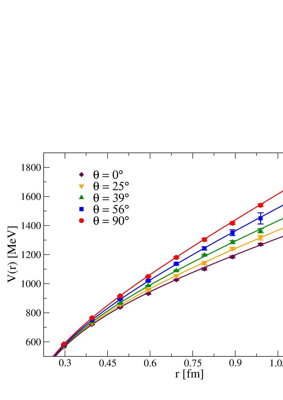
In Fig. 4 we show the results obtained for the potential as a function of for different values of on the finest, lattice. A property of its angular dependence is clearly visible, which is present also for data on the coarser lattice and is in line with what observed in Ref. [21]: at fixed , the potential increases as the angle between the quark-antiquark separation and increases, and reaches its maximum in the plane orthogonal to .
A peculiar property that we found is that, as one tries to perform a best fit of data according to the ansatz given in Eq. (13), it is sufficient to include only the lowest order Fourier coefficient , for each parameter, in order to obtain a reasonable value of the reduced chi-squared test (see the caption of Table 3), and if further coefficients are inserted in the best fit, they come out to be compatible with zero within errors. The best fit function obtained for the finer lattice is displayed in Fig. 4 as a function of and , while in Fig. 5 the same best fit function is shown in a three dimensional plot. The anisotropy of the potential is better seen by looking at the contour plot in Fig. 6. The best fit parameters for both lattices are reported in Table 3, and in Fig. 7 we show the angular variation of the string tension, from which it is clear that a single cosine term well describes data in both cases.


| [MeV] | [MeV] | ||
|---|---|---|---|
| 0.493(6) | 414(2) | 644(5) | |
| 0.499(23) | 398(4) | 407(20) |
| -0.130(10) | 0.262(7) | -0.154(8) | |
| -0.323(64) | 0.351(32) | -0.428(52) |

Another interesting feature emerges from the data in Table 3: the constant term in the Cornell potential gets an angular dependence as well. This is a very peculiar feature, since that would imply an additive term in the potential which depends on but not on . However, we stress that the associated Fourier coefficient is reduced by a factor as one moves from the coarse to the fine lattice, consistently with the vanishing of such angular dependence in the continuum limit. Notice that an analogous consideration, i.e. the vanishing of the angular dependence in the continuum limit, could be made for the Coulomb coupling, but not for the string tension; a more detailed discussion of this issue will be done in the following subsection. Finally, we stress that most of the -dependence of the potential can be ascribed to Fourier coefficients, since the parameters , and , which are sort of averaged values over different directions, show just a mild variation with respect to the case.
Having determined that the full angular dependence of the static quark potential can be described just by the first non trivial harmonic term, we can determine all relevant parameters from an analysis of the potential along the directions parallel and orthogonal to , i.e. from , which are the standard quantities already explored in Ref. [21] and which have been extended in the present study to a finer lattice spacing and to different values of .
III.3 , : continuum extrapolated results
In this subsection, in order to perform a continuum extrapolation of the -dependence of the static potential, we consider numerical results obtained at different values of the magnetic field and of the lattice spacing, and mostly for quark-antiquark separation parallel () or orthogonal () to the magnetic field. That gives us access to the Cornell parameters in those directions, i.e. and , and , and , and . According to the analysis of the angular dependence given in the previous subsection, that provides us with enough information to characterize the complete behavior of the potential. Indeed, if for each parameter we introduce its anisotropy
| (14) |
and its average relative change with
| (15) |
we have, assuming that when ,
| (16) |
and
| (17) | ||||
i.e. such quantities are enough to fix all the coefficients giving a non-trivial contribution to Eq. (13). That would have not been possible without the assumption for .
Results obtained in this way for the coefficients at the various magnetic fields and lattice spacings are shown in Fig. 8, while in Fig. 9 we report results for the quantities . A remarkable feature is that this quantities show a very mild variation with the magnetic field, so that most of the dependence of the potential on can be ascribed to the anisotropy coefficients . Moreover, the signs of such anisotropies are always consistent with the fact that, at fixed , the potential has a minimum (maximum) for .
We performed a continuum limit extrapolation of our data according to the following ansatz
| (18) | ||||
which is similar to the one adopted in Ref. [21] and consists of a power law in for both set of quantities, with the insertion of corrections for all involved coefficients. Reasonable fits are obtained if the data on the coarsest lattice are discarded. Continuum extrapolated results are displayed in Fig. 8 and Fig. 9, while numerical results for the best fit parameters are reported in Table 4.
The results obtained for the coefficients show that, while the anisotropy of the string tension has a well defined non-zero continuum limit, with a value around 15 % for GeV2, those of the Coulomb coupling and of seem to disappear in the same limit. Indeed, reasonable best fits are obtained also by imposing and to vanish in the continuum limit ( and respectively for and ), while the same is not true for (). The continuum extrapolated results obtained for the ratios confirm, instead, that on average all Cornell parameters have little dependence on the magnetic field. Again, reasonable best fits are obtained also by imposing to be -independent in the continuum limit ( for , for , and for ).
In summary, the modification of the quark-antiquark potential induced by the magnetic field persists in the continuum limit, and this is mostly due to the anisotropy induced in the string tension. In order to directly compare with the analysis of Ref. [21], in Fig. 10 we report also results for the relative variation of the string tension along the and axis, together with their continuum extrapolations.


| 0.151(32) | 1.64(30) | 9.5/11 | |||
| 0.046(39) | 1.51(67) | 7.3/11 | |||
| 0.066(36) | 1.48(50) | 7.8/11 |

III.4 Anisotropic deconfinement in the large field limit?
The continuum extrapolation discussed in the previous subsection has been obtained for a range of magnetic fields going up to around 1 GeV2, however it is tempting to extrapolate it to larger values of . In particular, results obtained for the longitudinal string tension indicate that it would vanish for magnetic fields of the order of 4 GeV2: this is clearly visible from Fig. 11, where the continuum extrapolation for the ratio along the axes has been extended up to .
A vanishing string tension at some critical value of , corresponding to a sort of longitudinal deconfinement, would have important consequences, e.g. for the anisotropic propagation of heavy quark-antiquark pairs, and could be put in connection with theoretical speculations about anisotropic quantum transitions at large values of [98].
A question naturally arises at this point: how reliable is the extension to large magnetic fields of a continuum extrapolation obtained in a smaller range of ? Unfortunately, a direct continuum extrapolation for GeV2 is presently hindered by the large ultraviolet cut-off effects which are expected when [72]. This sets the limit GeV2 for two of the lattice spacings explored in the present study.
However, we can extend the range of explored just for the finest lattice spacing, fm, where GeV2. Therefore, we have performed further numerical simulations for and GeV2, obtaining the results for the string tension which are reported in Fig. 11. The new results follow roughly the extrapolation of the continuum band, thus proving that a steady increase of the anisotropy persists up to very large fields. On the other hand, understanding whether an anisotropic deconfinement really takes place at some critical value of requires further studies at finer values of the lattice spacing.

III.5 results
For finite temperature runs, we have extracted the static potential from the gauge invariant correlator of Polyakov loops, see Eqs. (6) and (7). In this case we report on results at a single value of the lattice spacing (the finest one, fm) and for three temperatures below the transition temperature, namely MeV (corresponding to lattices , respectively), where we still expect the system may exhibit confining properties. In the deconfined phase, instead, Polyakov loop correlators give access to various kind of gluonic screening masses: the effect of the magnetic field on those masses will be studied in a forthcoming investigation. In Fig. 12 we show the results obtained for at some values of the magnetic field, respectively for MeV and MeV. In general, we observe a behavior which is different from that present at .
The anisotropy is still visible, and goes in the same direction as for , with the potential for quark-antiquark separations parallel to being suppressed with respect to the orthogonal case. The anisotropy is more pronounced for large magnetic fields and for intermediate separations, while it disappears in the limit of large distances: this is actually expected, since the magnetic background cannot disrupt the cluster property of the theory, hence the correlation of two Polyakov loops must be independent, in the large distance limit, from the direction of their relative separation.


Contrary to the zero temperature case, the main effect of the magnetic field seems to be that of suppressing the potential in all directions. Only for relatively small magnetic fields (smaller and smaller as the temperature increases) the observed can be fitted according to a Cornell potential and is qualitatively similar to that observed for . However, in these cases one is not able to distinguish, within errors, the results obtained in the various directions: this is due to the larger statistical uncertainties affecting the Polyakov loop correlator, especially in the low temperature regime, where the Polyakov loop is more suppressed and the correlators are noisier. The results obtained for the string tension in such cases are reported in Fig. 13. As expected for vanishing , the string tension decreases as the temperature approaches the deconfinement transition. Such an effect comes out to be enhanced when the external field is turned on.
The observed behavior is consistent with the decrease of the chiral pseudocritical temperature which has been observed in previous studies [15, 17]. This phenomenon has been usually named as inverse magnetic catalysis, because of its relation with the behavior of the chiral condensate, which is an increasing function of at low (direct magnetic catalysis), and becomes non-monotonic around the transition, in association with a decrease of . Our observations provide evidence for a strong effect of the magnetic field also on the confining properties of the medium which, at fixed temperature, seem to be lost if the magnetic field is strong enough.
Actually, looking at the behavior of the chiral condensate for the same values of temperature and magnetic field, the effect on the confining properties seems to be the leading phenomenon. In Fig. 14 we report the renormalized light chiral condensate as a function of for the three explored temperatures, which is defined as [15]:
| (19) |
where the subtraction eliminates additive divergences, while the multiplication by the bare light quark mass takes care of multiplicative ones. It is clearly visible that, for the two lowest temperatures, no signal of inverse magnetic catalysis is visible in the explored range of , while in the same range we already observe a strong modification of the free energy of the static pair, such that we are not able to fit it according to a Cornell potential, something which we interpret as an effective disappearance of the confining properties.
This might have many interesting interpretations and consequences. First, from a theoretical point of view, the suppression of the confining properties seems to be a dominant phenomenon with respect to the effect of the magnetic field on the chiral condensate, so that one would be tempted to describe the observed decrease of with in terms of “deconfinement catalysis” rather than of “inverse magnetic catalysis”; notice that this point of view is also suggested by recent computations in holographic models [47]. Second, from a phenomenological point of view, the precocious modification of the confining properties induced by the magnetic background, might have significant consequences on the suppression of heavy quark bound states (e.g., ) to be observed in the thermal medium produced in non-central heavy ion collisions.
IV Conclusions
Following an explorative study [21], which showed the presence of strong effects on the confining properties of the QCD vacuum induced by the presence of an external magnetic background, we have performed a deeper investigation of the phenomenon, which has extended the previous analysis of Ref. [21] in various directions. We have thus studied the static potential for various orientations of the quark-antiquark separation with respect to the background field, in order to obtain information about its angular dependence. Then, exploiting new numerical simulations performed for finer values of the lattice spacing, we have extracted a continuum extrapolation of our results and tried to extend the analysis towards larger magnetic fields. As a byproduct of our study, we have also obtained a continuum extrapolation of the static potential at zero external field. Finally, we have extended our investigation at finite temperature, exploring the effects of the magnetic background below the pseudo-critical temperature . Our main results can be summarized as follows.
At zero temperature, the full angular dependence of the anisotropic potential can be described assuming that it has a Cornell form along each direction. Moreover, the angular dependence of the parameters can be accounted for by the first allowed term in a Fourier expansion in , which corresponds to a quadrupole deformation. On the other hand, the continuum extrapolation of our results shows that the magnetic field induces a significant anisotropy only for the string tension, while the Coulomb coupling is almost unaffected, at least for GeV2. The latter result is compatible with an analysis based on the numerical study of gluon field strength correlators [23].
The observed anisotropy of the potential suggests that the string tension in the direction parallel to the magnetic field might disappear for magnetic fields of the order of GeV2. While this extrapolation to large magnetic fields cannot be supported by a reliable continuum limit in that regime, we have verified that it is consistent with results obtained at the finest explored lattice spacing, where we managed to perform numerical simulations for magnetic fields up GeV2. Future numerical studies on finer lattices could check the hypothesis of a possible longitudinal deconfinement at large , which presently is just suggested by our results.
Finally, our finite temperature results, obtained in an interval
ranging approximately from 100 MeV to right below the pseudocritical
temperature, have shown that the main effect of the magnetic field on
the static potential in that range consists of a general suppression
of the string tension and of the confinining properties of the
medium. Moreover, such phenomenon happens even when still no
effect of inverse magnetic catalysis is visible in the chiral
condensate, thus suggesting that the decrease of the pseudocritical
temperature as a function of , usually named as “inverse magnetic
catalysis”, might be understood in terms of a “deconfinement
catalysis”, representing the leading physical phenomenon: this idea
is also supported by some recent computations
in holographic models [47].
From a phenomenological point of view,
the precocious disappearance of the confining properties
of the static potental might have a significant influence
on the suppression of heavy quark bound
states produced in the thermal medium, even below ,
in all situations in which a strong magnetic field might be present,
e.g. in non-central heavy ion collisions and in the thermal medium of
the early Universe. This is an issue of particular interest, which should
be further investigated in future studies.
Acknowledgements.
We acknowledge PRACE for awarding us access to resource FERMI based in Italy at CINECA, under project Pra09-2400 - SISMAF. FS received funding from the European Research Council under the European Community Seventh Framework Programme (FP7/2007-2013) ERC grant agreement No 279757. FN acknowledges financial support from the INFN SUMA project.References
- [1] V. Skokov, A. Y. Illarionov and V. Toneev, Int. J. Mod. Phys. A 24, 5925 (2009) [arXiv:0907.1396 [nucl-th]].
- [2] V. Voronyuk, V. D. Toneev, W. Cassing, E. L. Bratkovskaya, V. P. Konchakovski and S. A. Voloshin, Phys. Rev. C 83, 054911 (2011) [arXiv:1103.4239 [nucl-th]].
- [3] A. Bzdak and V. Skokov, Phys. Lett. B 710, 171 (2012) [arXiv:1111.1949 [hep-ph]].
- [4] W. -T. Deng and X. -G. Huang, Phys. Rev. C 85, 044907 (2012) [arXiv:1201.5108 [nucl-th]].
- [5] K. Tuchin, Adv. High Energy Phys. 2013, 490495 (2013) [arXiv:1301.0099].
- [6] R. Holliday and K. Tuchin, arXiv:1604.04572 [hep-ph].
- [7] T. Vachaspati, Phys. Lett. B 265, 258 (1991).
- [8] D. Grasso and H. R. Rubinstein, Phys. Rept. 348, 163 (2001) [astro-ph/0009061].
- [9] R. C. Duncan and C. Thompson, Astrophys. J. 392, L9 (1992).
- [10] D. E. Kharzeev, K. Landsteiner, A. Schmitt and H. U. Yee, Lect. Notes Phys. 871, 1 (2013).
- [11] V. A. Miransky and I. A. Shovkovy, Phys. Rept. 576, 1 (2015) [arXiv:1503.00732 [hep-ph]].
- [12] M. D’Elia, S. Mukherjee and F. Sanfilippo, Phys. Rev. D 82, 051501 (2010) [arXiv:1005.5365 [hep-lat]].
- [13] P. V. Buividovich, M. N. Chernodub, D. E. Kharzeev, T. Kalaydzhyan, E. V. Luschevskaya and M. I. Polikarpov, Phys. Rev. Lett. 105, 132001 (2010) [arXiv:1003.2180 [hep-lat]].
- [14] M. D’Elia and F. Negro, Phys. Rev. D 83, 114028 (2011) [arXiv:1103.2080 [hep-lat]].
- [15] G. S. Bali, F. Bruckmann, G. Endrodi, Z. Fodor, S. D. Katz, S. Krieg, A. Schafer and K. K. Szabo, JHEP 1202, 044 (2012) [arXiv:1111.4956 [hep-lat]].
- [16] E.-M. Ilgenfritz, M. Kalinowski, M. Muller-Preussker, B. Petersson and A. Schreiber, Phys. Rev. D 85, 114504 (2012) [arXiv:1203.3360 [hep-lat]].
- [17] G. S. Bali, F. Bruckmann, G. Endrodi, Z. Fodor, S. D. Katz and A. Schafer, Phys. Rev. D 86, 071502 (2012) [arXiv:1206.4205 [hep-lat]].
- [18] M. D’Elia, M. Mariti and F. Negro, Phys. Rev. Lett. 110, 082002 (2013) [arXiv:1209.0722 [hep-lat]].
- [19] F. Bruckmann, G. Endrodi and T. G. Kovacs, JHEP 1304, 112 (2013) [arXiv:1303.3972 [hep-lat]].
- [20] E.-M. Ilgenfritz, M. Muller-Preussker, B. Petersson and A. Schreiber, Phys. Rev. D 89, no. 5, 054512 (2014) [arXiv:1310.7876 [hep-lat]].
- [21] C. Bonati, M. D’Elia, M. Mariti, M. Mesiti, F. Negro and F. Sanfilippo, Phys. Rev. D 89, 114502 (2014) [arXiv:1403.6094 [hep-lat]].
- [22] A. Schäfer, G. Endrodi, and J. Wellnhofer, Phys. Rev. D 92, no. 1, 014509 (2015) [arXiv:1506.07698 [hep-lat]].
- [23] M. D’Elia, E. Meggiolaro, M. Mesiti and F. Negro, Phys. Rev. D 93, 054017 (2016) [arXiv:1510.07012 [hep-lat]].
- [24] C. Bonati, M. D’Elia, M. Mariti, F. Negro and F. Sanfilippo, Phys. Rev. D 89, no. 5, 054506 (2014) [arXiv:1310.8656 [hep-lat]]; Phys. Rev. Lett. 111, 182001 (2013) [arXiv:1307.8063 [hep-lat]].
- [25] L. Levkova and C. DeTar, Phys. Rev. Lett. 112, no. 1, 012002 (2014) [arXiv:1309.1142 [hep-lat]].
- [26] G. S. Bali, F. Bruckmann, G. Endrodi, F. Gruber and A. Schaefer, JHEP 1304, 130 (2013) [arXiv:1303.1328 [hep-lat]].
- [27] G. S. Bali, F. Bruckmann, G. Endrödi, S. D. Katz and A. Schaefer, JHEP 1408, 177 (2014) [arXiv:1406.0269 [hep-lat]].
- [28] P. Cea and L. Cosmai, JHEP 1512, 058 (2015) [arXiv:1509.01982 [hep-lat]].
- [29] M. M. Musakhanov and F. C. Khanna, hep-ph/9605232.
- [30] J. Rafelski, In *Sandansky 1998, Frontier tests of QED and physics of the vacuum* 425-439 [hep-ph/9806389].
- [31] H. T. Elze, B. Muller and J. Rafelski, hep-ph/9811372.
- [32] M. N. Chernodub, arXiv:1001.0570 [hep-ph].
- [33] M. Asakawa, A. Majumder and B. Muller, Phys. Rev. C 81, 064912 (2010) [arXiv:1003.2436 [hep-ph]].
- [34] B. V. Galilo and S. N. Nedelko, Phys. Rev. D 84, 094017 (2011) [arXiv:1107.4737 [hep-ph]].
- [35] M. A. Andreichikov, V. D. Orlovsky and Y. A. Simonov, Phys. Rev. Lett. 110, 162002 (2013) [arXiv:1211.6568 [hep-ph]].
- [36] T. Kojo and N. Su, Phys. Lett. B 720, 192 (2013) [arXiv:1211.7318 [hep-ph]].
- [37] T. Kojo and N. Su, Phys. Lett. B 726, 839 (2013) [arXiv:1305.4510 [hep-ph]].
- [38] P. Watson and H. Reinhardt, Phys. Rev. D 89, 045008 (2014) [arXiv:1310.6050 [hep-ph]].
- [39] J. O. Andersen, W. R. Naylor and A. Tranberg, JHEP 1404, 187 (2014) [arXiv:1311.2093 [hep-ph]].
- [40] S. Ozaki, Phys. Rev. D 89, 054022 (2014) [arXiv:1311.3137 [hep-ph]].
- [41] K. Kamikado and T. Kanazawa, JHEP 1403, 009 (2014) [arXiv:1312.3124 [hep-ph]].
- [42] N. Mueller, J. A. Bonnet and C. S. Fischer, Phys. Rev. D 89, 094023 (2014) [arXiv:1401.1647 [hep-ph]].
- [43] N. Mueller and J. M. Pawlowski, Phys. Rev. D 91, 116010 (2015) [arXiv:1502.08011 [hep-ph]].
- [44] E. S. Fraga and L. F. Palhares, Phys. Rev. D 86, 016008 (2012) [arXiv:1201.5881 [hep-ph]].
- [45] E. S. Fraga, J. Noronha and L. F. Palhares, Phys. Rev. D 87, no. 11, 114014 (2013) [arXiv:1207.7094 [hep-ph]].
- [46] R. Rougemont, R. Critelli and J. Noronha, Phys. Rev. D 93, no. 4, 045013 (2016) [arXiv:1505.07894 [hep-th]].
- [47] D. Dudal, D. R. Granado and T. G. Mertens, Phys. Rev. D 93, no. 12, 125004 (2016) [arXiv:1511.04042 [hep-th]].
- [48] R. L. S. Farias, V. S. Timoteo, S. S. Avancini, M. B. Pinto and G. Krein, arXiv:1603.03847 [hep-ph].
- [49] S. I. Finazzo, R. Critelli, R. Rougemont and J. Noronha, arXiv:1605.06061 [hep-ph].
- [50] B. McInnes, Nucl. Phys. B 906, 40 (2016) [arXiv:1511.05293 [hep-th]].
- [51] V. A. Miransky and I. A. Shovkovy, Phys. Rev. D 66, 045006 (2002) [hep-ph/0205348].
- [52] M. N. Chernodub, Mod. Phys. Lett. A 29, 1450162 (2014).
- [53] R. Rougemont, R. Critelli and J. Noronha, Phys. Rev. D 91, 066001 (2015) [arXiv:1409.0556 [hep-th]].
- [54] E. J. Ferrer, V. de la Incera and X. J. Wen, Phys. Rev. D 91, 054006 (2015) [arXiv:1407.3503 [nucl-th]].
- [55] Y. A. Simonov and M. A. Trusov, Phys. Lett. B 747, 48 (2015) [arXiv:1503.08531 [hep-ph]].
- [56] J. Alford and M. Strickland, Phys. Rev. D 88, 105017 (2013) [arXiv:1309.3003 [hep-ph]].
- [57] D. Dudal and T. G. Mertens, Phys. Rev. D 91, 086002 (2015) [arXiv:1410.3297 [hep-th]].
- [58] S. Cho, K. Hattori, S. H. Lee, K. Morita and S. Ozaki, Phys. Rev. D 91, 045025 (2015) [arXiv:1411.7675 [hep-ph]].
- [59] H. Taya, Phys. Rev. D 92, 014038 (2015) [arXiv:1412.6877 [hep-ph]].
- [60] C. Bonati, M. D’Elia and A. Rucci, Phys. Rev. D 92, 054014 (2015) [arXiv:1506.07890 [hep-ph]].
- [61] K. Hattori, T. Kojo and N. Su, Nucl. Phys. A 951, 1 (2016) [arXiv:1512.07361 [hep-ph]].
- [62] K. Suzuki and T. Yoshida, Phys. Rev. D 93, 051502 (2016) [arXiv:1601.02178 [hep-ph]]; arXiv:1607.04935 [hep-ph].
- [63] X. Guo, S. Shi, N. Xu, Z. Xu and P. Zhuang, Phys. Lett. B 751, 215 (2015) [arXiv:1502.04407 [hep-ph]].
- [64] K. Fukushima, K. Hattori, H. U. Yee and Y. Yin, Phys. Rev. D 93, no. 7, 074028 (2016) [arXiv:1512.03689 [hep-ph]].
- [65] P. Gubler, K. Hattori, S. H. Lee, M. Oka, S. Ozaki and K. Suzuki, Phys. Rev. D 93, no. 5, 054026 (2016) [arXiv:1512.08864 [hep-ph]].
- [66] P. Weisz, Nucl. Phys. B 212, 1 (1983).
- [67] G. Curci, P. Menotti and G. Paffuti, Phys. Lett. B 130, 205 (1983) [Erratum-ibid. B 135, 516 (1984)].
- [68] C. Morningstar and M. J. Peardon, Phys. Rev. D 69, 054501 (2004) [hep-lat/0311018].
- [69] G. ’t Hooft, Nucl. Phys. B 153, 141 (1979).
- [70] P. H. Damgaard and U. M. Heller, Nucl. Phys. B 309, 625 (1988).
- [71] M. H. Al-Hashimi and U. J. Wiese, Ann. Phys. 324, 343 (2009) [arXiv:0807.0630 [quant-ph]].
- [72] M. D’Elia, Lect. Notes Phys. 871, 181 (2013) [arXiv:1209.0374 [hep-lat]].
- [73] Y. Aoki, S. Borsanyi, S. Durr, Z. Fodor, S. D. Katz, S. Krieg and K. K. Szabo, JHEP 0906, 088 (2009) [arXiv:0903.4155 [hep-lat]].
- [74] S. Borsanyi, G. Endrodi, Z. Fodor, A. Jakovac, S. D. Katz, S. Krieg, C. Ratti and K. K. Szabo, JHEP 1011, 077 (2010) [arXiv:1007.2580 [hep-lat]];
- [75] S. Borsanyi, Z. Fodor, C. Hoelbling, S. D. Katz, S. Krieg and K. K. Szabo, Phys. Lett. B 730, 99 (2014) [arXiv:1309.5258 [hep-lat]].
- [76] M. A. Clark, A. D. Kennedy and Z. Sroczynski, Nucl. Phys. Proc. Suppl. 140, 835 (2005) [hep-lat/0409133].
- [77] M. A. Clark and A. D. Kennedy, Phys. Rev. Lett. 98, 051601 (2007) [hep-lat/0608015].
- [78] M. A. Clark and A. D. Kennedy, Phys. Rev. D 75, 011502 (2007) [hep-lat/0610047].
- [79] A. Hasenfratz and F. Knechtli, Phys. Rev. D 64, 034504 (2001) [hep-lat/0103029].
- [80] M. Albanese et al. [APE Collaboration], Phys. Lett. B 192 (1987) 163.
- [81] M. Della Morte, A. Shindler and R. Sommer, JHEP 0508, 051 (2005) [hep-lat/0506008].
- [82] L. S. Brown and W. I. Weisberger, Phys. Rev. D 20, 3239 (1979).
- [83] L. D. McLerran and B. Svetitsky, Phys. Rev. D 24, 450 (1981).
- [84] S. Nadkarni, Phys. Rev. D 34, 3904 (1986).
- [85] O. Kaczmarek, F. Karsch, P. Petreczky and F. Zantow, Phys. Lett. B 543, 41 (2002) [hep-lat/0207002].
- [86] O. Jahn and O. Philipsen, Phys. Rev. D 70, 074504 (2004) [hep-lat/0407042].
- [87] G. Rossi and M. Testa, Phys. Rev. D 87, 085014 (2013) [arXiv:1304.2542 [hep-lat]].
- [88] E. Eichten, K. Gottfried, T. Kinoshita, J. B. Kogut, K. D. Lane and T. M. Yan, Phys. Rev. Lett. 34, 369 (1975) [Erratum-ibid. 36, 1276 (1976)].
- [89] R. Sommer, Nucl. Phys. B 411, 839 (1994) [hep-lat/9310022].
- [90] B. Blossier et al. [ETM Collaboration], JHEP 0907, 043 (2009) [arXiv:0904.0954 [hep-lat]].
- [91] R. Baron et al. [ETM Collaboration], JHEP 1008, 097 (2010) [arXiv:0911.5061 [hep-lat]].
- [92] P. Fritzsch, F. Knechtli, B. Leder, M. Marinkovic, S. Schaefer, R. Sommer and F. Virotta, Nucl. Phys. B 865, 397 (2012) [arXiv:1205.5380 [hep-lat]].
- [93] G. S. Bali et al., Nucl. Phys. B 866, 1 (2013) [arXiv:1206.7034 [hep-lat]]
- [94] C. T. H. Davies et al. [HPQCD Collaboration], Phys. Rev. D 81, 034506 (2010) [arXiv:0910.1229 [hep-lat]].
- [95] A. Bazavov et al., Phys. Rev. D 85, 054503 (2012) doi:10.1103/PhysRevD.85.054503 [arXiv:1111.1710 [hep-lat]].
- [96] C. Aubin et al., Phys. Rev. D 70, 094505 (2004) doi:10.1103/PhysRevD.70.094505 [hep-lat/0402030].
- [97] S. Aoki et al., arXiv:1607.00299 [hep-lat].
- [98] M. N. Chernodub, Phys. Rev. Lett. 106, 142003 (2011) doi:10.1103/PhysRevLett.106.142003 [arXiv:1101.0117 [hep-ph]]; Phys. Rev. D 82, 085011 (2010) doi:10.1103/PhysRevD.82.085011 [arXiv:1008.1055 [hep-ph]].