跳到论文正文
W Papers独立论文阅读器 arXiv:1607.08109 论文正文 计算阅读时间 · 0%
引用这篇论文根据当前论文元数据生成,正式投稿前建议核对。


License: arXiv.org perpetual non-exclusive license
arXiv:1607.08109v2 [quant-ph] 10 Aug 2016

Irreversible Evolution of a Wave Packet in The Rigged Hilbert Space Quantum Mechanics.

Giulia Marcucci Affiliation: Institute for Complex Systems, National Research Council (ISC-CNR), Via dei Taurini 19, 00185 Rome (IT). Email: marcucci.giulia@gmail.com    Claudio Conti Affiliation: Institute for Complex Systems, National Research Council (ISC-CNR), Via dei Taurini 19, 00185 Rome (IT). Affiliation: Department of Physics, University Sapienza, Piazzale Aldo Moro 5, 00185 Rome (IT). URL: http://www.complexlight.org
August 24, 2026
Abstract

It is well known that a state with complex energy cannot be the eigenstate of a self-adjoint operator, as the Hamiltonian. Resonances, i.e. states with exponentially decaying observables, are not vectors belonging to the conventional Hilbert space. One can describe these resonances in an unusual mathematical formalism, based on the so-called Rigged Hilbert Space (RHS). In the RHS, the states with complex energy are denoted as Gamow Vectors (GV), and they model decay processes.

We study GV of the Reversed Harmonic Oscillator (RHO), and we analytically and numerically investigate the unstable evolution of wave packets. We introduce the background function to study initial data not composed only by a summation of GV and we analyse different wave packets belonging to specific function spaces. Our work furnishes support to the idea that irreversible wave propagations can be investigated using Rigged Hilbert Space Quantum Mechanics and provides insights for the experimental investigation of irreversible dynamics.

I Introduction

The spontaneous decay of nuclear particles, or the empirical evidences for the Big Bang, lead various authors [1, 2, 3, 4, 5, 4] to consider modifications of the principles of quantum mechanics in order to include time-asymmetry. Despite a long standing effort, the need for these modifications is still debated. However, the debate stimulated the developments of theoretical tools and paradigms by a growing community of scientists. These tools recently found surprisingly applications in nonlinear physics and photonics [6, 7, 8].

The time-asimmetric dynamics of quantum systems are also relevant in biophysics, fluid dynamics, network theory, entanglement generation and epigenetic studies (see for example [9, 10, 11] and the references therein). The decay from local maxima in the energetic landscape of complex systems is generically retained irreversible. However the origin of this irreversibility in the case of microscopic quantum structures, or in quantum inspired models of networks [12], is unconsidered so far [13].

The leading theoretical background of Time-Asymmetric Quantum Mechanics (TA-QM) is the RHS, an enlarged Hilbert space, which includes non-normalizable wave packets that get amplified, or decay exponentially with time. The paradigmatic model for TA-QM is the reversed harmonic oscillator (RHO). Whithin standard QM the description of the evolution of a wavefunction may be done by using the continuous spectrum of the Hamiltonian. In TA-QM one considers a RHS, and generalized eigenvalues with complex energies do have physical meanings [14]. The corresponding non-normalizable eigenvectors are the so-called “Gamow vectors” [15, 16] and form a numerable generalized basis for integrable functions. This discrete resummation of the continuous spectrum furnishes novel physical insights for the spontaneous decay of a wave packet. For example, one can predict the surprising result of the quantization of the decay rates, which has been experimentally observed in an optical emulation [7, 17].

A further intriguing outcome of the TA-QM is the fact that it unveils a particular structure in the phase space. Namely, one can discriminate initial data in terms of their projection on the eigenvectors of the RHO continuous spectrum. These projections engender different vector subspaces depending on specific Hardy spaces. The question if this classification has direct physical counterpart has no answer at the moment, albeit mathematically this has important implications. If the initial wavefunction belongs to a particular space, it is completely represented by a numerable set of generalized eigenfunctions. On the contrary, the representation is given in terms of a finite number of GV and a background function.

Despite these mathematical properties have been studied by several authors [18, 19, 20, 21, 22, 23, 24, 25], a direct physical evidence of their implications is lacking, even in the simplest case of RHO. In this manuscript, we review the basics of TA-QM and of the GV approach to the RHO. Moreover, we study the way the function space of the input wavefunctions has a direct counterpart in the long term evolution.

This article is organized as follows: in sec. II we present three theorems which establish that quantum mechanics with a temporal asymmetry cannot exist in the standard Hilbert space formulation. In sec. III we build a different topology for the space of initial data and show the way this new geometry causes an enlargement of the Hilbert space, namely, the rigged Hilbert space. Direct consequences of RHS are disclosed in sec. IV. In sec. V we describe quantized damped motion, and in sec. VI we study RHO. In sec. VII and VIII we study the evolution of a function with compact support and a Gaussian function, respectively. We show the differences between their propagation: since the first one belongs to a specific function space, it exponentially decays with time; on the contrary, since the Gaussian function does not have a compact support, it is the superposition of exponentially and algebraically decaying waves. Conclusions are drawn in sec. IX.

II Fundamental theorems of QM

In order to build a mathematical theory behind a generic quantum system we need to define a Hausdorff vector space Ψ\Psi, with a locally convex topology τ\tau and a scalar product (⋅|⋅)(\cdot|\cdot). We need also an algebra 𝒜\mathcal{A} of τ\tau-continuous linear operator on Ψ\Psi and a probability measure 𝒫\mathcal{P} on 𝒜\mathcal{A}. By the scalar product (⋅|⋅)(\cdot|\cdot), we are able to build a norm ‖ψ‖=(ψ|ψ)||\psi||=\sqrt{(\psi|\psi)} ∀ψ∈Ψ\forall\psi\in\Psi and a metric d⁡(ψ,ϕ)=‖ϕ−ψ‖d(\psi,\phi)=||\phi-\psi|| ∀ϕ,ψ∈Ψ\forall\,\phi,\psi\in\Psi, that is induced by the norm, therefore we can settle a new topology τd\tau_{d} on Ψ\Psi, given by the distance dd. Now, we have a Euclidean space (Ψ,τd)(\Psi,\tau_{d}), which is also normed and separable. To be a physical space needs the completeness.

Let (ℋ,τℋ)(\mathcal{H},\tau_{\mathcal{H}}) be the completion of (Ψ,τd)(\Psi,\tau_{d}); ℋ\mathcal{H} is a separable Hilbert space, and is the space used to formulate the known time symmetric quantum theory. The temporal simmetry in a Hilbert space arises from the following three theorems:

Theorem II.1 (Gleason).

[26] For every probability 𝒫⁡(Λ)\mathcal{P}(\Lambda), there exists a positive trace class operator ρ\rho such that

𝒫⁡(Λ)=T​r​(Λ​ρ).\mathcal{P}(\Lambda)=Tr(\Lambda\rho).
Theorem II.2 (Stone-Neumann).

[27] Let us consider the Schrödinger-Neumann equation for ρ\rho previously defined

∂ρ⁡(t)∂t=iℏ​[H,ρ​(t)],\frac{\partial\rho(t)}{\partial t}=\frac{i}{\hbar}[H,\rho(t)],

with HH Hamiltonian operator. The solutions of such an equation are time simmetric and they are given by the group of unitary operators U†​(t)=exp−iℏ​H​tU^{\dagger}(t)=\exp{-\frac{i}{\hbar}Ht}.

Theorem II.3 (Hegerfeldt).

[28] For every Hermitian and semi-bounded Hamiltonian HH, either

T​r​(Λ⁡(t)​ρ)=T​r​(Λ​ρ​(t))=0​∀t∈ℝTr(\Lambda(t)\rho)=Tr(\Lambda\rho(t))=0\;\;\forall t\in\mathbb{R}

or

T​r​(Λ⁡(t)​ρ)=T​r​(Λ​ρ​(t))>0​∀t∈ℝTr(\Lambda(t)\rho)=Tr(\Lambda\rho(t))>0\;\;\forall t\in\mathbb{R}

except on a set of Lebesgue measure zero.

These theorems imply that time asymmetric solutions of the Schrödinger equation

i​ℏ​∂ϕ⁡(t)∂t=H​ϕ​(t)i\hbar\frac{\partial\phi(t)}{\partial t}=H\phi(t)

with time asymmetric boundary conditions are not allowed, hence we need to modify the mathematical description of the system.

III Rigged Hilbert Space Topology

For every fixed ψ0∈Ψ\psi_{0}\in\Psi, the translation T:Ψ→ΨT:\Psi\rightarrow\Psi such that ψ→ψ+ψ0\psi\rightarrow\psi+\psi_{0} is a linear homeomorphism of Ψ\Psi on itself. Therefore τ\tau is uniquely determined by the neighborhood system I⁡(0)I(0) centered at the origin, because every other neighborhood of any point ψ\psi of Ψ\Psi is obtained by translating a neighborhood of the origin of the vector ψ\psi. (Ψ,τ)(\Psi,\tau) is said to be locally convex if 𝒞={C∈I⁡(0)∣C​ is convex}\mathcal{C}=\{C\in I(0)\;\mid\;C\mbox{ is convex}\} is a neighborhood local basis. Since every open ball centered at the origin is convex, it is also a member of 𝒞\mathcal{C} if and only if ∃A∈τ| 0∈A⊂Br​(0)​∀Br​(0)\exists A\in\tau\;\mid\;0\in A\subset B_{r}(0)\;\forall B_{r}(0). By this last condition, we build a locally convex topology τ\tau on Ψ\Psi that is finer than the topology τd\tau_{d} induced by the norm.

Let us suppose that (Ψ,τ)(\Psi,\tau) and (ℋ,τℋ)(\mathcal{H},\tau_{\mathcal{H}}) are the previously described spaces and, besides, τ\tau is locally convex and finer than τℋ\tau_{\mathcal{H}}. Then we can define another completion Φ\Phi of Ψ\Psi, this time with respect to τ\tau, and find another complete space (Φ,τΦ)(\Phi,\tau_{\Phi}) that is different from (ℋ,τℋ)(\mathcal{H},\tau_{\mathcal{H}}). Precisely, Φ⊂ℋ\Phi\subset\mathcal{H}, and Φ\Phi is dense in ℋ\mathcal{H}. Moreover, Φ⊂ℋ⇒ℋ∗⊂Φ∗\Phi\subset\mathcal{H}\Rightarrow\mathcal{H}^{*}\subset\Phi^{*}, where ℋ∗\mathcal{H}^{*} and Φ∗\Phi^{*} are the dual spaces of ℋ\mathcal{H} and Φ\Phi, respectively.

The definition of dual space is the basis to build a RHS and we need a more physically accessible dual space, according to [1] and [2]. Let ℰ\mathcal{E} be a Euclidean space. We identify the scalar product on ℰ\mathcal{E} as (⋅|⋅)(\cdot|\cdot); instead ⟨⋅|⋅⟩\langle\cdot|\cdot\rangle is the operatorial product on the dual space ℰ∗\mathcal{E}^{*}, namely F⁡(v)=⟨F|v⟩F(v)=\langle F|v\rangle. We define our dual space Φ×\Phi^{\times} as the space of antilinear and continuous functionals on Φ\Phi, that is

F∈Φ×⟺F⁡(ϕ)=⟨ϕ|F⟩.F\in\Phi^{\times}\;\Longleftrightarrow\;F(\phi)=\langle\phi|F\rangle.

Thus every functional in Φ×\Phi^{\times} has a sort of complex conjugate in Φ∗\Phi^{*}, and the Riesz-Frechet representation theorem on the Hilbert space ℋ\mathcal{H} still works, hence ℋ=ℋ×\mathcal{H}=\mathcal{H}^{\times}. In this manner we obtain the Gelfand triplet Φ⊂ℋ⊂Φ×\Phi\subset\mathcal{H}\subset\Phi^{\times}, which defines our RHS.

IV Gamow Vectors

It is well known that, in order to be observable, the Hamiltonion operator HH of a quantum system must be self-adjoint on ℋ\mathcal{H}, so H=H†H=H^{\dagger}. Nevertheless H≠H×H\neq H^{\times} on Φ×\Phi^{\times}.

Let us consider the secular equation

H×​|E⟩=E​|E⟩.H^{\times}|E\rangle=E|E\rangle. (1)

If |E⟩∈Φ×∖ℋ|E\rangle\in\Phi^{\times}\setminus\mathcal{H}, we cannot affirm that the corresponding eigenvalue EE is a real number. We define a generalized eigenvector |E⟩∈Φ×|E\rangle\in\Phi^{\times}, which has complex eigenvalue, as a Gamow vector |ϕnG⟩=|En±⟩=|ER±i​Γn2⟩|\phi_{n}^{G}\rangle=|E_{n}^{\pm}\rangle=|E_{R}\pm i\frac{\Gamma_{n}}{2}\rangle (subscript RR is due to one of the first applications of this theory, that Bohm developed in scattering experiments [1], and it is related to the resonances of the system). From the Schrödinger equation (in units such that ℏ=1\hbar=1), we get a unitary operator U⁡(t)=e−i​H​tU(t)=e^{-iHt} for the temporal evolution of any state in ℋ\mathcal{H}. We see that U​(t)×=ei​H×​tU(t)^{\times}=e^{iH^{\times}t} is not unitary on Φ×\Phi^{\times}:

U​(t)×​|ER±i​Γn2⟩=ei​ER​t​e∓Γn2​t​|ER±i​Γn2⟩,U(t)^{\times}|E_{R}\pm i\frac{\Gamma_{n}}{2}\rangle=e^{iE_{R}t}e^{\mp\frac{\Gamma_{n}}{2}t}|E_{R}\pm i\frac{\Gamma_{n}}{2}\rangle, (2)

U​(t)×U(t)^{\times} is not an isometry, because

‖U​(t)×​|ER±i​Γn2⟩‖2=e∓Γn​t​‖|ER±i​Γn2⟩‖2.||U(t)^{\times}|E_{R}\pm i\frac{\Gamma_{n}}{2}\rangle||^{2}=e^{\mp\Gamma_{n}t}|||E_{R}\pm i\frac{\Gamma_{n}}{2}\rangle||^{2}. (3)

Moreover

‖U​(t)×​|ER±i​Γn2⟩‖⟶t→±∞0||U(t)^{\times}|E_{R}\pm i\frac{\Gamma_{n}}{2}\rangle||\stackrel{{\scriptstyle t\rightarrow\pm\infty}}{{\longrightarrow}}0 (4)

and

‖U​(t)×​|ER±i​Γn2⟩‖⟶t→∓∞+∞.||U(t)^{\times}|E_{R}\pm i\frac{\Gamma_{n}}{2}\rangle||\stackrel{{\scriptstyle t\rightarrow\mp\infty}}{{\longrightarrow}}+\infty. (5)

In a physical context, we need to identify Φ\Phi with the Schwartz space S⁡(ℝN)S(\mathbb{R}^{N}), that is, the space of rapidly decreasing functions, and the Hilbert space ℋ\mathcal{H} with the space of quadratically integrable functions ℒ2​(ℝN)\mathcal{L}^{2}(\mathbb{R}^{N}), so these last two expressions suggest that we need to define the following new spaces:

Φ−={ϕ∈Φ∣f⁡(E)=⟨ϕ|E−⟩∈S⁡(ℝ)∩ℋ−2},\Phi_{-}=\left\{\phi\in\Phi\mid f(E)=\langle\phi|E^{-}\rangle\in S(\mathbb{R})\cap\mathcal{H}_{-}^{2}\right\},
Φ+={ϕ∈Φ∣f⁡(E)=⟨ϕ|E+⟩∈S⁡(ℝ)∩ℋ+2};\Phi_{+}=\left\{\phi\in\Phi\mid f(E)=\langle\phi|E^{+}\rangle\in S(\mathbb{R})\cap\mathcal{H}_{+}^{2}\right\};

where ℋ−2\mathcal{H}_{-}^{2} and ℋ+2\mathcal{H}_{+}^{2} are Hardy spaces bounded from below and from above, respectively. To sum up, Φ±\Phi_{\pm} are dense in Φ\Phi, Φ=Φ−+Φ+\Phi=\Phi_{-}+\Phi_{+} (Φ−∩Φ+≠0\Phi_{-}\cap\Phi_{+}\neq 0 generally) and Φ\Phi is dense in ℋ\mathcal{H}, consequently

Φ−⊂d​e​n​s​eΦ⊂d​e​n​s​eℋ⊂d​e​n​s​eΦ×⊂d​e​n​s​eΦ−×,\Phi_{-}\stackrel{{\scriptstyle\scriptscriptstyle{dense}}}{{\subset}}\Phi\stackrel{{\scriptstyle\scriptscriptstyle{dense}}}{{\subset}}\mathcal{H}\stackrel{{\scriptstyle\scriptscriptstyle{dense}}}{{\subset}}\Phi^{\times}\stackrel{{\scriptstyle\scriptscriptstyle{dense}}}{{\subset}}\Phi_{-}^{\times}, (6)
Φ+⊂d​e​n​s​eΦ⊂d​e​n​s​eℋ⊂d​e​n​s​eΦ×⊂d​e​n​s​eΦ+×.\Phi_{+}\stackrel{{\scriptstyle\scriptscriptstyle{dense}}}{{\subset}}\Phi\stackrel{{\scriptstyle\scriptscriptstyle{dense}}}{{\subset}}\mathcal{H}\stackrel{{\scriptstyle\scriptscriptstyle{dense}}}{{\subset}}\Phi^{\times}\stackrel{{\scriptstyle\scriptscriptstyle{dense}}}{{\subset}}\Phi_{+}^{\times}. (7)

We have now found two Gelfand triplets, Φ−⊂ℋ⊂Φ−×\Phi_{-}\subset\mathcal{H}\subset\Phi_{-}^{\times} and Φ+⊂ℋ⊂Φ+×\Phi_{+}\subset\mathcal{H}\subset\Phi_{+}^{\times}, where the evolution operator U⁡(t)U(t) acts as a semigroup, because it is well defined and continuous only for t≤0t\leq 0 on Φ−\Phi_{-}, and only for t≥0t\geq 0 on Φ+\Phi_{+}. The value t=0t=0 expresses the intrinsic irreversibility we have when, for example, we divide an experiment into a preparation stage and a registration stage. In this case, Φ−\Phi_{-} will be the space of the initial states and Φ+\Phi_{+} will be the space of the detected states.

V Quantization of a Damped Motion

For its simplicity and its relevance, the harmonic oscillator (HO) can be chosen to introduce the study of quantum mechanics in a time symmetric context [18, 19]. The classical HO Hamiltonian is

H=p22​m+m​ω22​x2.H=\frac{p^{2}}{2m}+\frac{m\omega^{2}}{2}x^{2}.

We quantize the HO by converting the canonical coordinates x,px,p into the operators x^,p^\hat{x},\hat{p} such that

[x^,p^]=i​ℏ,[\hat{x},\hat{p}]=i\hbar,

and we find the spectrum of HH:

H​ψ​(x)=E​ψ​(x),En=ℏ​ω​(n+12),H\psi(x)=E\psi(x),\;\;E_{n}=\hbar\omega\left(n+\frac{1}{2}\right),
ψn​(x)=m​ωℏ​π4​12n​n!​Hn​(m​ωℏ​x),\psi_{n}(x)=\sqrt[4]{\frac{m\omega}{\hbar\pi}}\frac{1}{\sqrt{2^{n}n!}}H_{n}\left(\sqrt{\frac{m\omega}{\hbar}}x\right), (8)

where Hn​(x)=(−1)n​x2​dnd​xn​e−x2H_{n}(x)=(-1)^{n}x^{2}\frac{d^{n}}{dx^{n}}e^{-x^{2}} are the Hermite polynomials.

In a time asymmetric context, considering the equation of a damped motion comes natural for its inherent irreversibility. In fact, if we consider the classical dynamical system in one dimension

{dd​t​u​(t)=−γ​u​(t)u⁡(0)=u0\left\{\begin{array}[]{c}\frac{d}{dt}u(t)=-\gamma u(t)\\ u(0)=u_{0}\end{array}\right. (9)

where γ>0\gamma>0 and m=ℏ=1m=\hbar=1, we have

u⁡(t)=e−γ​t​u0,u(t)=e^{-\gamma t}u_{0},

which represents a damping for t≥0t\geq 0. We quantize it exactly as we did for the HO, even if this one is not a Hamiltonian system. In a general nn-dimensional space, one defines a dynamical system as

d​ud​t=X⁡(u),\frac{du}{dt}=X(u),

where XX is a vector field. Using canonical coordinates (u1,…,un,v1,…,vn)(u^{1},...,u^{n},v^{1},...,v^{n}), we get the Hamiltonian

H⁡(u,v)=∑k=1nvk​Xk​(u),H(u,v)=\sum_{k=1}^{n}v_{k}X_{k}(u),

where XkX_{k} are the components of XX in the coordinate basis, so for Eq.(9)

H⁡(u,v)=−γ​u​v.H(u,v)=-\gamma uv.

Since the quantization must take into account that v^\hat{v} does not commute with u^\hat{u}, we have

H^​(u^,v^)=−γ2​(u^​v^+v^​u^).\hat{H}(\hat{u},\hat{v})=-\frac{\gamma}{2}(\hat{u}\hat{v}+\hat{v}\hat{u}). (10)

By performing the canonical transformation

u^=γ​x^−p^2​γ,v^=γ​x^+p^2​γ,\hat{u}=\frac{\gamma\hat{x}-\hat{p}}{\sqrt{2\gamma}},\;\;\;\hat{v}=\frac{\gamma\hat{x}+\hat{p}}{\sqrt{2\gamma}}, (11)

one obtains the Hamiltonian of the reversed harmonic oscillator (RHO):

H^​(x^,p^)=p^22−γ2​x^22.\hat{H}(\hat{x},\hat{p})=\frac{\hat{p}^{2}}{2}-\frac{\gamma^{2}\hat{x}^{2}}{2}. (12)

Let us compare the HO and the RHO. We pass from the first one to the second one, by changing ω\omega into the complex value i​γi\gamma [24]. This simple transformation allows to move from a parabolic potential bounded from below to a parabolic barrier. This potential overturning produces a completely different physics: the HO models the behavior of a pointlike mass around a stable equilibrium and the RHO gives the dynamics around an unstable equilibrium, an intrinsically irreversible evolution (at variance with an oscillator, a falling body never goes back to its initial position).

In this section, we analyze the Hamiltonian of the damped motion, defined in (10). As proved in [18], H^​(u^,v^)\hat{H}(\hat{u},\hat{v}) is self-adjoint on ℒ2​(ℝ)\mathcal{L}^{2}(\mathbb{R}) and parity invariant. We define the time reversal operator TT such that

T​ϕ​(t):=ϕ⁡(−t)⇒T​U​(t)=U†​(t)​T⇒U⁡(t)​T​U​(t)=T,T\phi(t):=\phi(-t)\;\;\Rightarrow TU(t)=U^{\dagger}(t)T\;\;\Rightarrow U(t)TU(t)=T,

where U⁡(t):=e−i​H​tU(t):=e^{-iHt}. TT plays a fundamental role in this system, and coincides with the inverse Fourier transformation, i.e. T​ϕ​(u,t):=Fˇ​[ϕ]​(u,t)T\phi(u,t):=\check{F}[\phi](u,t),where

Fˇ​[ϕ]​(x,t)=12​π​∫ℝei​k​x​ϕ​(k,t)​𝑑k.\check{F}[\phi](x,t)=\frac{1}{\sqrt{2\pi}}\int_{\mathbb{R}}e^{ikx}\phi(k,t)dk.

Let us define two families of tempered distributions in Φ×\Phi^{\times}, the first one

u^​|f0−⟩:=0,f0−​(u)=δ⁡(u),\hat{u}|f_{0}^{-}\rangle:=0,\;\;\;\;f_{0}^{-}(u)=\delta(u),
∀n∈ℕ⁡|fn−⟩:=(−i)nn!​v^n​|f0−⟩⇒\forall n\in\mathbb{N}\;\;\;|f_{n}^{-}\rangle:=\frac{(-i)^{n}}{\sqrt{n!}}\hat{v}^{n}|f_{0}^{-}\rangle\;\;\Rightarrow (13)
⇒fn−​(u)=(−1)nn!​dnd​un​δ​(u);\Rightarrow\;\;f_{n}^{-}(u)=\frac{(-1)^{n}}{\sqrt{n!}}\frac{d^{n}}{du^{n}}\delta(u);

and the second one

v^​|f0+⟩:=0,f0+​(u)=1,\hat{v}|f_{0}^{+}\rangle:=0,\;\;\;\;f_{0}^{+}(u)=1,
∀n∈ℕ⁡|fn+⟩:=1n!​u^n​|f0+⟩⇒fn+​(u)=unn!.\forall n\in\mathbb{N}\;\;\;|f_{n}^{+}\rangle:=\frac{1}{\sqrt{n!}}\hat{u}^{n}|f_{0}^{+}\rangle\;\;\Rightarrow\;\;f_{n}^{+}(u)=\frac{u^{n}}{\sqrt{n!}}. (14)

Hereafter, following [1, 2, 3], we denote a tempered distribution fn±f_{n}^{\pm} a resonance. We can see that

H×​|fn±⟩=±En​|fn±⟩,H^{\times}|f_{n}^{\pm}\rangle=\pm E_{n}|f_{n}^{\pm}\rangle,

where En:=i​γ​(n+12)∈ℂE_{n}:=i\gamma\left(n+\frac{1}{2}\right)\in\mathbb{C}. Given that fn±f_{n}^{\pm} are tempered distributions, their inverse Fourier transforms are well defined, and they are

Fˇ​[fn−]=in2​π​fn+,\check{F}[f_{n}^{-}]=\frac{i^{n}}{\sqrt{2\pi}}f_{n}^{+}, (15)
Fˇ​[fn+]=in​2​π​fn−.\check{F}[f_{n}^{+}]=i^{n}\sqrt{2\pi}f_{n}^{-}. (16)

We show the quasi-orthogonality and the quasi-completeness of the resonances:

⟨fn−|fm+⟩=δn,m,\langle f_{n}^{-}|f_{m}^{+}\rangle=\delta_{n,m},
∑n=0∞fn−​(u)​fn+​(y)=δ⁡(u−y).\sum_{n=0}^{\infty}f_{n}^{-}(u)f_{n}^{+}(y)=\delta(u-y).

In order to find real energy values, we need to analyze also the continuous spectrum. Since HH is parity invariant, each generalized eigenvalue is doubly degenerate, thus

H×​ψ±E=E​ψ±E.H^{\times}\psi_{\pm}^{E}=E\psi_{\pm}^{E}.

As one can see in [18], the generalized eigenfunctions are

ψ±E​(u)=12​π​γ​u±−(i​Eγ+12),\psi_{\pm}^{E}(u)=\frac{1}{\sqrt{2\pi\gamma}}u_{\pm}^{-\left(\frac{iE}{\gamma}+\frac{1}{2}\right)}, (17)

where u±λu_{\pm}^{\lambda} are tempered distributions such that

u+λ:={uλu≥00u<0,u_{+}^{\lambda}:=\left\{\begin{array}[]{cc}u^{\lambda}&u\geq 0\\ 0&u<0\end{array}\right.,
u−λ:={0u<0uλu≤0.u_{-}^{\lambda}:=\left\{\begin{array}[]{cc}0&u<0\\ u^{\lambda}&u\leq 0\end{array}\right..

It is possible to prove both the orthonormality and the completeness of the eigenfunctions, namely

∑±∫[ψ±E1​(u)]∗​ψ±E2​(u)​𝑑u=δ⁡(E1−E2);\sum_{\pm}\int[\psi_{\pm}^{E_{1}}(u)]^{*}\psi_{\pm}^{E_{2}}(u)du=\delta(E_{1}-E_{2});
∑±∫[ψ±E​(u)]∗​ψ±E​(u′)​𝑑E=δ⁡(u−u′).\sum_{\pm}\int[\psi_{\pm}^{E}(u)]^{*}\psi_{\pm}^{E}(u^{\prime})dE=\delta(u-u^{\prime}).

Therefore we can apply the Gelfand-Maurin theorem [23] and write any function in S⁡(ℝ)S(\mathbb{R}) as

ϕ⁡(u)=∑±∫ψ±E​(u)​⟨ϕ|ψ±E⟩∗​𝑑E.\phi(u)=\sum_{\pm}\int\psi_{\pm}^{E}(u)\langle\phi|\psi_{\pm}^{E}\rangle^{*}dE.

By repeating the same reasoning

H×​Fˇ​[ψ±−E]=E​Fˇ​[ψ±−E],H^{\times}\check{F}\left[\psi_{\pm}^{-E}\right]=E\check{F}\left[\psi_{\pm}^{-E}\right], (18)

so one can prove also the orthonormality and the completeness of the inverse Fourier transforms of the eigenfunctions, whence

ϕ⁡(u)=∑±∫Fˇ​[ψ±−E]​(u)​⟨ϕ|Fˇ​[ψ±−E]⟩∗​𝑑E.\phi(u)=\sum_{\pm}\int\check{F}\left[\psi_{\pm}^{-E}\right](u)\langle\phi|\check{F}\left[\psi_{\pm}^{-E}\right]\rangle^{*}dE. (19)

We have just defined two groups of eigenfunctions, ψ±E​(u)\psi_{\pm}^{E}(u) and Fˇ​[ψ±−E]​(u)\check{F}\left[\psi_{\pm}^{-E}\right](u), which represent the continuous spectrum of the Hamiltonian of a damped motion into the RHS. Moreover, we have just seen that they depend on the tempered distributions u±−(i​Eγ+12)u_{\pm}^{-\left(\frac{iE}{\gamma}+\frac{1}{2}\right)}, which have simple poles in the complex plane when

E=−En=−i​γ​(n+12).E=-E_{n}=-i\gamma\left(n+\frac{1}{2}\right).

Thanks to the properties of the generalized function u±λu_{\pm}^{\lambda} [18], we can finally state what follows:

R​e​s​[ψ±E,−En]=(±1)n​i​γ2​π​n!​fn−,Res\left[\psi_{\pm}^{E},-E_{n}\right]=\frac{(\pm 1)^{n}i\sqrt{\gamma}}{\sqrt{2\pi n!}}f_{n}^{-}, (20)
R​e​s​[Fˇ​[ψ±−E],En]=(±i)n​i​γ2​π​n!​fn+.Res\left[\check{F}[\psi_{\pm}^{-E}],E_{n}\right]=\frac{(\pm i)^{n}i\sqrt{\gamma}}{2\pi\sqrt{n!}}f_{n}^{+}. (21)

By defining the following spaces, we get two Gelfand triplets:

ℋ=ℒ2​(ℝ),\mathcal{H}=\mathcal{L}^{2}(\mathbb{R}),
Φ=S⁡(ℝ),\Phi=S(\mathbb{R}),
Φ−={ϕ∈Φ∣f⁡(E)=⟨ϕ|Fˇ​[ψ±−E]⟩∈ℋ−2},\Phi_{-}=\left\{\phi\in\Phi\mid f(E)=\langle\phi|\check{F}[\psi_{\pm}^{-E}]\rangle\in\mathcal{H}_{-}^{2}\right\}, (22)
Φ+={ϕ∈Φ∣f⁡(E)=⟨ϕ|ψ±E⟩∈ℋ+2},\Phi_{+}=\left\{\phi\in\Phi\mid f(E)=\langle\phi|\psi_{\pm}^{E}\rangle\in\mathcal{H}_{+}^{2}\right\}, (23)

where ℋ+2\mathcal{H}_{+}^{2} (ℋ+2\mathcal{H}_{+}^{2}) is the Hardy space on the upper (lower) complex half-plane, respectively.

From this framework into the RHS Φ×\Phi^{\times}, we can infer the irreversible evolution of certain waves in Φ\Phi. We established above the connection between the continuous and the point spectrum. Now we make this link definitively clear and we show that the evolution operator acts as a semigroup on Φ±\Phi_{\pm} for a well-defined orientation of the arrow of time. By recalling Eqs.(20) and (21), we apply the residue theorem to initial data in Φ±\Phi_{\pm} [18] and get two different expansions in GV:

ϕ+​(u)=∑n=0+∞⟨ϕ+|fn+⟩​fn−​(u)​∀ϕ+∈Φ+;\phi^{+}(u)=\sum_{n=0}^{+\infty}\langle\phi^{+}|f_{n}^{+}\rangle f_{n}^{-}(u)\;\;\forall\;\phi^{+}\in\Phi_{+};
ϕ−​(u)=∑n=0+∞⟨ϕ−|fn−⟩​fn+​(u)​∀ϕ−∈Φ−.\phi^{-}(u)=\sum_{n=0}^{+\infty}\langle\phi^{-}|f_{n}^{-}\rangle f_{n}^{+}(u)\;\;\forall\;\phi^{-}\in\Phi_{-}.

Thanks to the following definitions of two new function spaces, both of them subspaces of S⁡(ℝ)S(\mathbb{R}) and isomorphic by the inverse Fourier transformation, we can establish the relation between Φ+\Phi_{+} and Φ−\Phi_{-}:
𝒟=Cc∞​(ℝ)\mathcal{D}=C_{c}^{\infty}(\mathbb{R}) is the space of the infinitely differentiable functions with compact support;
𝒵={Fˇ​[ϕ]|ϕ∈𝒟}\mathcal{Z}=\left\{\check{F}[\phi]\,|\,\phi\in\mathcal{D}\right\}, where Fˇ\check{F} is the inverse Fourier transformation.
Since for each function ϕ∈𝒵\phi\in\mathcal{Z}, we have

ϕ⁡(u)=∑n=0+∞1n!​dnd​un​ϕ​(u)|u=0​un=∑n=0+∞fn+​(u)​⟨fn−|ϕ⟩,\phi(u)=\sum_{n=0}^{+\infty}\frac{1}{n!}\frac{d^{n}}{du^{n}}\phi(u)|_{u=0}u^{n}=\sum_{n=0}^{+\infty}f_{n}^{+}(u)\langle f_{n}^{-}|\phi\rangle,

while, at the same time, every ψ∈𝒟\psi\in\mathcal{D} is the Fourier transform of a function in 𝒵\mathcal{Z}, hence

ψ⁡(u)=12​π​∫ℝFˇ​[ψ]​(v)​e−i​v​u​𝑑v=∑n=0+∞fn−​(u)​⟨fn+|ψ⟩.\psi(u)=\frac{1}{\sqrt{2\pi}}\int_{\mathbb{R}}\check{F}[\psi](v)e^{-ivu}dv=\sum_{n=0}^{+\infty}f_{n}^{-}(u)\langle f_{n}^{+}|\psi\rangle.

We can state that

Φ+≡𝒟,Φ−≡𝒵.\Phi_{+}\equiv\mathcal{D},\;\;\Phi_{-}\equiv\mathcal{Z}. (24)

At last, we study the evolution operator U⁡(t)=e−i​H​tU(t)=e^{-iHt}. UU is a unitary group on ℋ=ℒ2​(ℝ)\mathcal{H}=\mathcal{L}^{2}(\mathbb{R}), given that if ψ⁡(u,0)∈ℒ2​(ℝ)\psi(u,0)\in\mathcal{L}^{2}(\mathbb{R}) then

ψ⁡(u,t)=U⁡(t)​ψ​(u,0)=eγ2​t​ψ​(eγ​t​u,0),\psi(u,t)=U(t)\psi(u,0)=e^{\frac{\gamma}{2}t}\psi(e^{\gamma t}u,0), (25)

transformation that turns out to be an isometry on ℒ2​(ℝ)\mathcal{L}^{2}(\mathbb{R}). This means that if ψ⁡(u,t)\psi(u,t) solves the Schrödinger equation, then also T​ψ​(u,t)=ψ⁡(u,−t)T\psi(u,t)=\psi(u,-t) does. Therefore the theory is time-reversal invariant on the Hilbert space ℋ\mathcal{H}, without letting us see the damping we expected. Where do we observe the temporal irreversibility? It lacks the analysis of UU restricted to Φ±\Phi_{\pm}. If ϕ+​(u,0)∈Φ+\phi^{+}(u,0)\in\Phi_{+} then

⟨U⁡(t)​ϕ+​|ψ±E⟩=⟨ϕ+|​U×​(t)​ψ±E⟩=\langle U(t)\phi^{+}|\psi_{\pm}^{E}\rangle=\langle\phi^{+}|U^{\times}(t)\psi_{\pm}^{E}\rangle=
=ei​E​t​⟨ϕ+|ψ±E⟩∈ℋ+2⇔t≥0;=e^{iEt}\langle\phi^{+}|\psi_{\pm}^{E}\rangle\;\in\mathcal{H}^{2}_{+}\;\;\Leftrightarrow\;\;t\geq 0;

on the other hand, if ϕ−​(u,0)∈Φ−\phi^{-}(u,0)\in\Phi_{-} then

⟨U⁡(t)​ϕ−|Fˇ​[ψ±−E]⟩=⟨U⁡(−t)​Fˇ​[ϕ−]|ψ±−E⟩=\langle U(t)\phi^{-}|\check{F}[\psi_{\pm}^{-E}]\rangle=\langle U(-t)\check{F}[\phi^{-}]|\psi_{\pm}^{-E}\rangle=
=⟨Fˇ​[ϕ+]|U×​(−t)​ψ±−E⟩=ei​E​t​⟨Fˇ​[ϕ−]|ψ±−E⟩==\langle\check{F}[\phi^{+}]|U^{\times}(-t)\psi_{\pm}^{-E}\rangle=e^{iEt}\langle\check{F}[\phi^{-}]|\psi_{\pm}^{-E}\rangle=
=ei​E​t​⟨ϕ−|Fˇ​[ψ±−E]⟩∈ℋ−2⇔t≤0.=e^{iEt}\langle\phi^{-}|\check{F}[\psi_{\pm}^{-E}]\rangle\;\in\mathcal{H}^{2}_{-}\;\;\Leftrightarrow\;\;t\leq 0.

We conclude that U⁡(t)U(t) establishes two semigroups:

U+​(t):Φ+⟶Φ+​∀t≥0U_{+}(t):\Phi_{+}\longrightarrow\Phi_{+}\;\;\;\forall t\geq 0

and

U−​(t):Φ−⟶Φ−​∀t≤0.U_{-}(t):\Phi_{-}\longrightarrow\Phi_{-}\;\;\;\forall t\leq 0.

We have just found a way to model irreversible phenomena. In fact, the action of UU allows to choose an orientation of the temporal arrow: if it goes forward from zero, then our initial data is in Φ+\Phi_{+}, otherwise it is in Φ−\Phi_{-}, indeed

ϕ+​(u,t)=∑ne−γ⁡(n+1/2)​t​⟨ϕ+|fn+⟩​fn−​(u)\phi^{+}(u,t)=\sum_{n}e^{-\gamma(n+1/2)t}\langle\phi^{+}|f_{n}^{+}\rangle f_{n}^{-}(u)

and

ϕ−​(u,t)=∑neγ⁡(n+1/2)​t​⟨ϕ−|fn−⟩​fn+​(u).\phi^{-}(u,t)=\sum_{n}e^{\gamma(n+1/2)t}\langle\phi^{-}|f_{n}^{-}\rangle f_{n}^{+}(u).

Moreover, all the physics we get fixing a specific orientation of time’s arrow is achievable fixing the other one too, because time reversal operator TT establishes an isomorphism between Φ+\Phi_{+} and Φ−\Phi_{-}, in fact

T​ϕ+​(u,t)=U⁡(−t)​T​ϕ+​(u,0)=ϕ−​(u,−t).T\phi^{+}(u,t)=U(-t)T\phi^{+}(u,0)=\phi^{-}(u,-t).

Summarizing, we got an irreversible quantum system by observing that the evolution operator acts as a semigroup on Φ±\Phi_{\pm}, due to the presence of resonant states fn±f_{n}^{\pm}. In this way, the instant t=0t=0 separates the evolution in two complementary directions: if one starts from Φ+\Phi_{+}, one can stays forever in Φ+\Phi_{+} only evolving forward in time. In other words one chooses the temporal orientation, fixes the signature of Φ±\Phi_{\pm}, and cannot go backwards.

Refer to caption
Figure 1: (Color online) Pictorial representation of Gelfand triplet defined in Eq.(7). Here Φ+≡𝒟\Phi_{+}\equiv\mathcal{D}, Φ≡S⁡(ℝ)\Phi\equiv S(\mathbb{R}) and ℋ≡ℒ2​(ℝ)\mathcal{H}\equiv\mathcal{L}^{2}(\mathbb{R}). One can get an Euler-Venn diagram also for the triplet in Eq.(6) by changing Φ+\Phi_{+} with Φ−\Phi_{-} and 𝒟\mathcal{D} with 𝒵\mathcal{Z}.

VI The Reversed Harmonic Oscillator:
Remarkable Results

We consider the family of operators [19]

V^λ=exp⁡{λ2​(x^​p^+p^​x^)}.\hat{V}_{\lambda}=\exp\left\{\frac{\lambda}{2}(\hat{x}\hat{p}+\hat{p}\hat{x})\right\}.

In a system of measurement where ℏ=1\hbar=1, we have
[x^,p^]=i[\hat{x},\hat{p}]=i, so

V^λ​ϕ​(x)=e−i​λ2​ϕ​(e−i​λ​x),\hat{V}_{\lambda}\phi(x)=e^{-i\frac{\lambda}{2}}\phi(e^{-i\lambda}x),

whence

V^λ​x^​V^λ−1=e−i​λ​x^\hat{V}_{\lambda}\hat{x}\hat{V}_{\lambda}^{-1}=e^{-i\lambda}\hat{x}

and

V^λ​p^​V^λ−1=ei​λ​p^.\hat{V}_{\lambda}\hat{p}\hat{V}_{\lambda}^{-1}=e^{i\lambda}\hat{p}.

If we recall the Hamiltonian in the equation (8)

HH​O:=p^22+γ2​x^22,H_{HO}:=\frac{\hat{p}^{2}}{2}+\frac{\gamma^{2}\hat{x}^{2}}{2},

it is easy to see that

V^±π4​H​V^±π4−1=±i​HH​O\hat{V}_{\pm\frac{\pi}{4}}H\hat{V}_{\pm\frac{\pi}{4}}^{-1}=\pm iH_{HO}

and we can transform the results we already know for the HO in results for the RHO:

EnH​O=γ⁡(n+12),En=i​EnH​O∈ℂE_{n}^{HO}=\gamma(n+\frac{1}{2}),\,E_{n}=iE_{n}^{HO}\,\in\,\mathbb{C}
ψnH​O=(γπ)1/4(2nn!)−1/2e−γ2​x2Hn(γx)\psi_{n}^{HO}=\left(\frac{\gamma}{\pi}\right)^{1/4}(2^{n}n!)^{-1/2}e^{-\frac{\gamma}{2}x^{2}}H_{n}(\sqrt{\gamma}x)
fn±=V^±π4−1​ψnH​O∈S×​(ℝ).f_{n}^{\pm}=\hat{V}_{\pm\frac{\pi}{4}}^{-1}\psi_{n}^{HO}\in S^{\times}(\mathbb{R}).

VI.1 The Unitary Transformation:
from (u,v)(u,v) to (x,p)(x,p) Framework

One passes from the HO to the RHO through the operator V^±π4\hat{V}_{\pm\frac{\pi}{4}}, but can also pass from H⁡(u^,v^)H(\hat{u},\hat{v}) to H⁡(x^,p^)H(\hat{x},\hat{p}), i.e. from the damped motion to the RHO, through a canonical transformation and find a relation between the spectra of these two Hamiltonians.

The canonical transformation from (u,v)(u,v) to (x,p)(x,p) it is generated by the generating function

S⁡(x,u)=γ2​x2−2​γ​x​u+12​u2,S(x,u)=\frac{\gamma}{2}x^{2}-\sqrt{2\gamma}xu+\frac{1}{2}u^{2}, (26)

with p=∂S∂xp=\frac{\partial S}{\partial x}, v=−∂S∂uv=-\frac{\partial S}{\partial u}.

We define the unitary transformation

𝒰:ℒ2​(ℝ)⟶ℒ2​(ℝ)\mathcal{U}:\mathcal{L}^{2}(\mathbb{R})\longrightarrow\mathcal{L}^{2}(\mathbb{R}) (27)

such that

f⁡(u)⟶(𝒰​f)​(x)=C~​∫ℝf⁡(u)​ei​S​(x,u)​𝑑u,f(u)\longrightarrow(\mathcal{U}f)(x)=\tilde{C}\int_{\mathbb{R}}f(u)e^{iS(x,u)}du,

with C~:=e−i​π8​γ2​π24\tilde{C}:=e^{-i\frac{\pi}{8}}\sqrt[4]{\frac{\gamma}{2\pi^{2}}} and we can prove that 𝒰\mathcal{U} is unitary by demonstrating that

|C~|2​∫ℝei⁡[S⁡(x,u)−S⁡(x′,u)]​𝑑u=δ⁡(x−x′).|\tilde{C}|^{2}\int_{\mathbb{R}}e^{i[S(x,u)-S(x^{\prime},u)]}du=\delta(x-x^{\prime}).

In order to get a relation of quasi-orthogonality and quasi-completeness for the resonances, we need to understand the nature of the operator V^λ\hat{V}_{\lambda}. It acts almost like the evolution operator UU in Eq.(25), with a complex (instead of real) exponential, but this is enough only to say that V^λ\hat{V}_{\lambda} is unitary for pure imaginary λ\lambda, not for every λ∈ℂ\lambda\in\mathbb{C}. In fact, for a generic λ=ω+i​γ\lambda=\omega+i\gamma, where ω,γ∈ℝ\omega,\gamma\in\mathbb{R}, one has

⟨V^λ​ϕ|V^λ​ψ⟩=∫ℝd​x​[eγ−i​ω2​ϕ​(eγ−i​ω​x)]∗​eγ−i​ω2​ψ​(eγ−i​ω​x)=\langle\hat{V}_{\lambda}\phi|\hat{V}_{\lambda}\psi\rangle=\int_{\mathbb{R}}dx\left[e^{\frac{\gamma-i\omega}{2}}\phi\left(e^{\gamma-i\omega}x\right)\right]^{*}e^{\frac{\gamma-i\omega}{2}}\psi\left(e^{\gamma-i\omega}x\right)=
=ei​ω​∫ℝd​x​[ϕ⁡(x)]∗​ψ​(x)=ei​ω​⟨ϕ|ψ⟩.=e^{i\omega}\int_{\mathbb{R}}dx\left[\phi(x)\right]^{*}\psi(x)=e^{i\omega}\langle\phi|\psi\rangle.

Therefore it is not surprising that fn±f_{n}^{\pm} are only proportional to 𝒰⁡[fn±​(u)]​(x)\mathcal{U}[f_{n}^{\pm}(u)](x) and not exactly equal. In fact

fn±​(x)=ei​n​π4​(2​π)±14​𝒰​[fn±​(u)]​(x).f_{n}^{\pm}(x)=e^{in\frac{\pi}{4}}(2\pi)^{\pm\frac{1}{4}}\mathcal{U}[f_{n}^{\pm}(u)](x).

Nevertheless, we achieve the same relation of quasi-orthogonality and quasi-completeness we had before:

⟨fn±​(x)|fm∓​(x)⟩=δn​m;\langle f_{n}^{\pm}(x)|f_{m}^{\mp}(x)\rangle=\delta_{nm};
∑n=0+∞[fn±​(x)]∗​fn∓​(x′)=δ⁡(x−x′).\sum_{n=0}^{+\infty}\left[f_{n}^{\pm}(x)\right]^{*}f_{n}^{\mp}(x^{\prime})=\delta(x-x^{\prime}).

Moreover

[fn±​(x)]∗=fn∓​(x).\left[f_{n}^{\pm}(x)\right]^{*}=f_{n}^{\mp}(x).

Recalling the equations (15), (16) and the meaning of the inverse Fourier transform for the damped motion represented by H^​(u^,v^)\hat{H}(\hat{u},\hat{v}) (the inverse Fourier transform coincides with the time reversal operator TT in that system), one has T=CT=C, where CC is the complex conjugation operator, as shown in [19].

We want to find χE\chi^{E} such that

H​χE=E​χE.H\chi^{E}=E\chi^{E}.

From [19] we get the complete derivation of the following solutions:

χ+E​(x)=C~2​π​γ​iν+12​Γ​(ν+1)​D−ν−1​(−−2​γ​i​x),\chi_{+}^{E}(x)=\frac{\tilde{C}}{\sqrt{2\pi\gamma}}i^{\frac{\nu+1}{2}}\Gamma(\nu+1)D_{-\nu-1}(-\sqrt{-2\gamma i}x),
χ−E​(x)=χ+E​(−x),\chi_{-}^{E}(x)=\chi_{+}^{E}(-x),

where here ν=−(i​Eγ+12)\nu=-\left(i\frac{E}{\gamma}+\frac{1}{2}\right) and

Dν​(z):=e−z24Γ⁡(−ν)​∫ℛξ±−ν−1​e∓z​ξ−12​ξ2​𝑑ξD_{\nu}(z):=\frac{e^{-\frac{z^{2}}{4}}}{\Gamma(-\nu)}\int_{\mathcal{R}}\xi_{\pm}^{-\nu-1}e^{\mp z\xi-\frac{1}{2}\xi^{2}}d\xi

is a Whittaker function [29].

If one remembers the equation (18), one knows that the set of eigenfunction is not complete yet. In fact, the two families of functions η±E​(x):=(𝒰​Fˇ​[ψ±−E])​(x)\eta_{\pm}^{E}(x):=\left(\mathcal{U}\check{F}[\psi_{\pm}^{-E}]\right)(x) still miss, and we obtain

H​η±E=−E​η±E,H\eta_{\pm}^{E}=-E\eta_{\pm}^{E},
η+E​(x)=C~2​π​γ​iν+12​Γ​(−ν)​Dν​(−2​γ​i​x),\eta_{+}^{E}(x)=\frac{\tilde{C}}{\sqrt{2\pi\gamma}}i^{\frac{\nu+1}{2}}\Gamma(-\nu)D_{\nu}(-\sqrt{2\gamma i}x),
η−E​(x)=η+E​(−x).\eta_{-}^{E}(x)=\eta_{+}^{E}(-x).

We observe that

η±E​(x)=[χ±E​(x)]∗,\eta_{\pm}^{E}(x)=[\chi_{\pm}^{E}(x)]^{*},

fact which confirms that the time reversal operator TT acts like the complex conjugation CC.

From the corresponding properties satisfied by ψ±E​(u)\psi_{\pm}^{E}(u) and from the unitary nature of 𝒰\mathcal{U} we have

∑±∫ℝ[χ±E​(x)]∗​χ±E′​(x)​𝑑x=δ⁡(E−E′);\sum_{\pm}\int_{\mathbb{R}}[\chi_{\pm}^{E}(x)]^{*}\chi_{\pm}^{E^{\prime}}(x)dx=\delta(E-E^{\prime});
∑±∫ℝ[χ±E​(x)]∗​χ±E​(x′)​𝑑E=δ⁡(x−x′);\sum_{\pm}\int_{\mathbb{R}}[\chi_{\pm}^{E}(x)]^{*}\chi_{\pm}^{E}(x^{\prime})dE=\delta(x-x^{\prime});
∑±∫ℝ[η±E​(x)]∗​η±E′​(x)​𝑑x=δ⁡(E−E′);\sum_{\pm}\int_{\mathbb{R}}[\eta_{\pm}^{E}(x)]^{*}\eta_{\pm}^{E^{\prime}}(x)dx=\delta(E-E^{\prime});
∑±∫ℝ[η±E​(x)]∗​η±E​(x′)​𝑑E=δ⁡(x−x′).\sum_{\pm}\int_{\mathbb{R}}[\eta_{\pm}^{E}(x)]^{*}\eta_{\pm}^{E}(x^{\prime})dE=\delta(x-x^{\prime}).

At this point, we have all the tools we need to study the analytic properties of these four families of eigenfunctions. The outcome is that χ±E​(x)\chi_{\pm}^{E}(x) and η±E​(x)\eta_{\pm}^{E}(x) have simple poles at E=−EnE=-E_{n} and E=EnE=E_{n}, respectively. Furthermore,

R​e​s​[χ±E​(x);−En]=C~2​π​γ​(−1)nn!​i−n2​Dn​(∓−2​γ​i​x),Res[\chi_{\pm}^{E}(x);-E_{n}]=\frac{\tilde{C}}{\sqrt{2\pi\gamma}}\frac{(-1)^{n}}{n!}i^{-\frac{n}{2}}D_{n}(\mp\sqrt{-2\gamma i}x),
R​e​s​[η±E​(x);En]=C~2​π​γ​(−1)nn!​in+12​Dn​(∓2​γ​i​x).Res[\eta_{\pm}^{E}(x);E_{n}]=\frac{\tilde{C}}{\sqrt{2\pi\gamma}}\frac{(-1)^{n}}{n!}i^{\frac{n+1}{2}}D_{n}(\mp\sqrt{2\gamma i}x).

In [29], [30] and [31] one can find out that
Dn​(y)=2−n2​e−y24​Hn​(z2)D_{n}(y)=2^{-\frac{n}{2}}e^{-\frac{y^{2}}{4}}H_{n}\left(\frac{z}{\sqrt{2}}\right). This, together with Hn​(−y)=(−1)n​Hn​(y)H_{n}(-y)=(-1)^{n}H_{n}(y), allows us to obtain

R​e​s​[χ±E​(x);−En]∝fn+​(x)Res[\chi_{\pm}^{E}(x);-E_{n}]\propto f_{n}^{+}(x)

and

R​e​s​[η±E​(x);En]∝fn−​(x).Res[\eta_{\pm}^{E}(x);E_{n}]\propto f_{n}^{-}(x).

Following section V, we get Φ±\Phi_{\pm} from the residues of the RHO eigenfunctions:

ℋ=ℒ2​(ℝ),\mathcal{H}=\mathcal{L}^{2}(\mathbb{R}),
Φ=S⁡(ℝ),\Phi=S(\mathbb{R}),
Φ−={ϕ∈Φ∣f⁡(E)=⟨ϕ|η±E⟩∈ℋ−2},\Phi_{-}=\left\{\phi\in\Phi\mid f(E)=\langle\phi|\eta_{\pm}^{E}\rangle\in\mathcal{H}_{-}^{2}\right\},
Φ+={ϕ∈Φ∣f⁡(E)=⟨ϕ|χ±E⟩∈ℋ+2}.\Phi_{+}=\left\{\phi\in\Phi\mid f(E)=\langle\phi|\chi_{\pm}^{E}\rangle\in\mathcal{H}_{+}^{2}\right\}.

VI.2 The Evolution Operator Acting like a Semigroup

We study waves ϕ±∈Φ±\phi_{\pm}\in\Phi_{\pm} and the action of the evolution operator. We have T=CT=C and

T⁡(Φ+)=Φ−.T(\Phi_{+})=\Phi_{-}.

Writing envelopes of ϕ±\phi_{\pm} in series of resonances:

ϕ+​(x)=∑n=0+∞⟨ϕ+|fn+⟩∗​fn−​(x)​∀ϕ+∈Φ+;\phi^{+}(x)=\sum_{n=0}^{+\infty}\langle\phi^{+}|f_{n}^{+}\rangle^{*}f_{n}^{-}(x)\;\;\forall\;\phi^{+}\in\Phi_{+};
ϕ−​(x)=∑n=0+∞⟨ϕ−|fn−⟩∗​fn+​(x)​∀ϕ−∈Φ−.\phi^{-}(x)=\sum_{n=0}^{+\infty}\langle\phi^{-}|f_{n}^{-}\rangle^{*}f_{n}^{+}(x)\;\;\forall\;\phi^{-}\in\Phi_{-}.

Thanks to the Gelfand-Maurin spectral theorem

ϕ+​(x)=∑±∫ℝd​E​χ±E​(x)​⟨ϕ+|ψ±E⟩∗\phi^{+}(x)=\sum_{\pm}\int_{\mathbb{R}}dE\chi_{\pm}^{E}(x)\langle\phi^{+}|\psi_{\pm}^{E}\rangle^{*}

and

ϕ−​(x)=∑±∫ℝd​E​η±E​(x)​⟨ϕ−|η±E⟩∗.\phi^{-}(x)=\sum_{\pm}\int_{\mathbb{R}}dE\eta_{\pm}^{E}(x)\langle\phi^{-}|\eta_{\pm}^{E}\rangle^{*}.

In conclusion, even in this case, the temporal evolution operator U⁡(t)=e−i​H​tU(t)=e^{-iHt} establishes a unitary group on ℋ=ℒ2​(ℝ)\mathcal{H}=\mathcal{L}^{2}(\mathbb{R}), and two semigroups:

U+​(t):Φ+⟶Φ+​∀t≥0;U_{+}(t):\Phi_{+}\longrightarrow\Phi_{+}\;\;\;\forall t\geq 0;
U−​(t):Φ−⟶Φ−​∀t≤0.U_{-}(t):\Phi_{-}\longrightarrow\Phi_{-}\;\;\;\forall t\leq 0.

Furthermore, if ϕ+​(x,0)∈Φ+\phi^{+}(x,0)\in\Phi_{+} then

ϕ+​(x,t)=∑ne−γ⁡(n+1/2)​t​⟨ϕ+|fn+⟩∗​fn−​(x),\phi^{+}(x,t)=\sum_{n}e^{-\gamma(n+1/2)t}\langle\phi^{+}|f_{n}^{+}\rangle^{*}f_{n}^{-}(x),

while, if ϕ−​(x,0)∈Φ−\phi^{-}(x,0)\in\Phi_{-} then

ϕ−​(x,t)=∑neγ⁡(n+1/2)​t​⟨ϕ−|fn−⟩∗​fn+​(x).\phi^{-}(x,t)=\sum_{n}e^{\gamma(n+1/2)t}\langle\phi^{-}|f_{n}^{-}\rangle^{*}f_{n}^{+}(x).

We stress again that we got an irreversible quantum theory by studying the action of UU on Φ±\Phi_{\pm} as a semigroup. Time t=0t=0 splits the evolution in two diametrically opposed directions, and it becomes the instant which separates two different dynamics.

VII Functions with Compact Support

In this section we examine a function set in Φ+\Phi_{+}. We start working in the (u,v)(u,v) representation, where H⁡(u^,v^)=−γ2​[u^​v^+v^​u^]H(\hat{u},\hat{v})=-\frac{\gamma}{2}[\hat{u}\hat{v}+\hat{v}\hat{u}]. We analyse the evolution in (u,v)(u,v) and (x,p)(x,p) planes. In (x,p)(x,p) the Hamiltonian is H=p^22−γ2​x^22H=\frac{\hat{p}^{2}}{2}-\frac{\gamma^{2}\hat{x}^{2}}{2} (we fix γ=1\gamma=1 hereafter).

VII.1 Wave Packets in (u,v)(u,v) Plane

We previously proved that Φ+\Phi_{+} and Φ−\Phi_{-} coincide with 𝒟\mathcal{D} and 𝒵\mathcal{Z}, respectively. We choose the forward orientation of the temporal arrow, so we focus our attention on the triplet

Φ+⊂ℋ⊂Φ+×,\Phi_{+}\subset\mathcal{H}\subset\Phi_{+}^{\times},

that is 𝒟⊂ℒ2​(ℝ)⊂𝒟×\mathcal{D}\subset\mathcal{L}^{2}(\mathbb{R})\subset\mathcal{D}^{\times}.

Let us consider the family of functions

ϕϵ​(u)={Kϵ​exp⁡[1(uϵ)2−1]|u|<ϵ0|u|≥ϵ\phi_{\epsilon}(u)=\left\{\begin{array}[]{cr}K_{\epsilon}\exp\left[\frac{1}{\left(\frac{u}{\epsilon}\right)^{2}-1}\right]&|u|<\epsilon\\ 0&|u|\geq\epsilon\end{array}\right. (28)

where ϵ>0\epsilon>0 and KϵK_{\epsilon} is such that ‖ϕϵ‖2=1||\phi_{\epsilon}||_{2}=1, i.e. (∫ℝ|ϕϵ​(u)|2​𝑑x)12=1\left(\int_{\mathbb{R}}|\phi_{\epsilon}(u)|^{2}dx\right)^{\frac{1}{2}}=1. ϕϵ​(u)\phi_{\epsilon}(u) is a function of class C∞​(ℝ)C^{\infty}(\mathbb{R}), precisely

ϕϵ​(u)∈𝒟​∀ϵ>0.\phi_{\epsilon}(u)\in\mathcal{D}\;\;\forall\,\epsilon>0.
Refer to caption
Figure 2: (Color online) Functions ϕϵ\phi_{\epsilon} with compact support defined in Eq.(28) for several ϵ\epsilon values.

Starting from

∑n=0∞fn−​(u)​fn+​(w)=δ⁡(u−w),\sum_{n=0}^{\infty}f_{n}^{-}(u)f_{n}^{+}(w)=\delta(u-w),

with fn−​(u)=(−1)nn!​dnd​un​δ​(u)f_{n}^{-}(u)=\frac{(-1)^{n}}{\sqrt{n!}}\frac{d^{n}}{du^{n}}\delta(u) and fn+​(u)=unn!f_{n}^{+}(u)=\frac{u^{n}}{\sqrt{n!}}, we have

ϕϵ​(u)=∫ℝd​w​δ​(u−w)​ϕϵ​(w)=\phi_{\epsilon}(u)=\int_{\mathbb{R}}dw\delta(u-w)\phi_{\epsilon}(w)=
=∫ℝd​w​∑n=0∞fn−​(u)​fn+​(w)​ϕϵ​(w)=∑n=0∞fn−​(u)​⟨ϕϵ|fn+⟩,=\int_{\mathbb{R}}dw\sum_{n=0}^{\infty}f_{n}^{-}(u)f_{n}^{+}(w)\phi_{\epsilon}(w)=\sum_{n=0}^{\infty}f_{n}^{-}(u)\langle\phi_{\epsilon}|f_{n}^{+}\rangle, (29)

since ϕϵ∈𝒟\phi_{\epsilon}\in\mathcal{D}. In deriving Eq.(29), as discussed in sec.V and in [19], the residue theorem allows to swap the integral and the summation. This is not valid for general functions in Φ\Phi not belonging to Φ+\Phi_{+}. We define the N-order background function as

ϕNB​G​(u,t):=ϕ⁡(u,t)−∑n=0Nfn−​(u)​⟨U⁡(t)​ϕ|fn+⟩∗∈Φ×;\phi_{N}^{BG}(u,t):=\phi(u,t)-\sum_{n=0}^{N}f_{n}^{-}(u)\langle U(t)\phi|f_{n}^{+}\rangle^{*}\;\in\;\Phi^{\times};

consequently

ϕ⁡(u,t)=∑n=0Nfn−​(u)​⟨U⁡(t)​ϕ|fn+⟩∗+ϕNB​G​(u,t)​∀ϕ∈Φ.\phi(u,t)=\sum_{n=0}^{N}f_{n}^{-}(u)\langle U(t)\phi|f_{n}^{+}\rangle^{*}+\phi_{N}^{BG}(u,t)\;\;\;\forall\phi\in\Phi.

For ϕ∈Φ+\phi\in\Phi_{+}, ϕN→+∞B​G=0\phi_{N\rightarrow+\infty}^{BG}=0 and U⁡(t)U(t) acts as a semigroup. The evolution is a superposition of exponentially decaying functions. On the contrary, for ϕ∉Φ+\phi\notin\Phi_{+}, ϕN→+∞B​G\phi_{N\rightarrow+\infty}^{BG} does not converge and the evolution includes non exponentially decaying components.

Refer to caption
Figure 3: (Color online) One-dimensional evolution of |ϕ1​(u,t)||\phi_{1}(u,t)| [Eq.(28) with ϵ=1\epsilon=1].
Refer to caption
Figure 4: (Color online) Evolution of |ϕ1​(u,t)||\phi_{1}(u,t)| [Eq.(28) with ϵ=1\epsilon=1].

We numerically simulate the Schrödinger equation i​∂ψ∂t=H​ψi\frac{\partial\psi}{\partial t}=H\psi for the Hamiltonian H=i​γ​(u​∂∂u+12)H=i\gamma\left(u\frac{\partial}{\partial u}+\frac{1}{2}\right) (with γ\gamma=1), with initial condition ψ⁡(u,t=0)=ϕϵ​(u)\psi(u,t=0)=\phi_{\epsilon}(u). Figures 3 and 4 show the resulting “focusing” evolution.

Figure 5 reports the evolution of the coefficients CN​(t):=⟨U⁡(t)​ϕ1|fN+⟩∗C_{N}(t):=\langle U(t)\phi_{1}|f_{N}^{+}\rangle^{*}. These brackets exponentially decay, with quantized decay rates. Into a semilogarithmic scale, the decay rates correspond to straight lines with different slopes.

Refer to caption
Figure 5: (Color online) Numerically calculated projections CN​(t):=⟨U⁡(t)​ϕ1|fN+⟩∗C_{N}(t):=\langle U(t)\phi_{1}|f_{N}^{+}\rangle^{*} on the N order resonances of a function with compact support [Eq.(28) with ϵ=1\epsilon=1] in the (u,v) representation, in a semilogarithmic scale.

VII.2 Wave Packets in (x,p)(x,p) Plane

We pass from the (u,v)(u,v) to (x,p)(x,p) by the unitary transformation 𝒰\mathcal{U}:

Refer to caption
Figure 6: (Color online) Transformed ϕϵ\phi_{\epsilon} [Eq.(30) for various ϵ\epsilon].
ϕϵ​(x)=𝒰⁡[ϕϵ​(u)]​(x)=∑n=0∞𝒰⁡[fn−​(u)]​(x)​⟨𝒰​ϕϵ|𝒰​fn+⟩=\phi_{\epsilon}(x)=\mathcal{U}[\phi_{\epsilon}(u)](x)=\sum_{n=0}^{\infty}\mathcal{U}[f_{n}^{-}(u)](x)\langle\mathcal{U}\phi_{\epsilon}|\mathcal{U}f_{n}^{+}\rangle=
=∑n=0∞fn−​(x)​⟨ϕϵ|fn+⟩,=\sum_{n=0}^{\infty}f_{n}^{-}(x)\langle\phi_{\epsilon}|f_{n}^{+}\rangle, (30)

with fn±​(x)=V^±π4−1​ψnH​O​(x)f_{n}^{\pm}(x)=\hat{V}_{\pm\frac{\pi}{4}}^{-1}\psi_{n}^{HO}(x).

We numerically analyse the transformed functions. In Fig. 6, one can see several (𝒰​ϕϵ)​(x)\left(\mathcal{U}\phi_{\epsilon}\right)(x). We remark that functions ϕϵ\phi_{\epsilon}, which have compact support in (u,v)(u,v), do not have compact support in (x,p)(x,p) phase plane.

Refer to caption
Figure 7: (Color online) One-dimensional evolution of a transformed function with compact support [Eq.(30), ϵ=1/2\epsilon=1/2] with a RHO potential.

We numerically study the evolution of wave packets in (x,p)(x,p). We solve numerically i​∂ψ∂t=H​ψi\frac{\partial\psi}{\partial t}=H\psi with initial condition ψ⁡(x,t=0)=(𝒰​ϕϵ)​(x)\psi(x,t=0)=\left(\mathcal{U}\phi_{\epsilon}\right)(x) and a RHO potential. Figures 7 and 8 show the resulting “defocusing” evolution.

Refer to caption
Figure 8: (Color online) Evolution of a transformed function with compact support [Eq.(30), ϵ=1/2\epsilon=1/2] with a RHO potential.

VIII Gaussian Function

We examine the Gelfand triplet in Eq.(7) defined in sections V and VI, in the case of the Gaussian function as element of the Hilbert space but not belonging neither to Φ+\Phi_{+} nor to Φ−\Phi_{-} (see figure 1). For this function, the expansion in Gamow states must be truncated and completed by an additional background function, not decaying exponentially, as discussed in sec. VII.1. We illustrate theoretically and numerically the properties of the background function, specifically studying a Gaussian function ϕ⁡(u)=e−u22π4\phi(u)=\frac{e^{-\frac{u^{2}}{2}}}{\sqrt[4]{\pi}} and its transformed 𝒰​[ϕ]​(x)\mathcal{U}[\phi](x). We analyse the evolution both in (u,v)(u,v) and (x,p)(x,p) planes.

VIII.1 The Background Function

Let us define a normalized Gaussian function

ϕ⁡(u)=1π4​e−u22∈S⁡(ℝ).\phi(u)=\frac{1}{\sqrt[4]{\pi}}e^{-\frac{u^{2}}{2}}\in S(\mathbb{R}). (31)

ϕ⁡(u)\phi(u) does not belong to 𝒟\mathcal{D} or to 𝒵\mathcal{Z} because the Fourier transformed of a Gaussian function is still a Gaussian function and 𝒟∩𝒵=∅\mathcal{D}\cap\mathcal{Z}=\emptyset.

Since ∑n=0+∞fn+​(u)​fn−​(w)=δ⁡(u−w)\sum_{n=0}^{+\infty}f_{n}^{+}(u)f_{n}^{-}(w)=\delta(u-w), we have

ϕ⁡(u)=∫ℝd​w​∑n=0+∞fn−​(u)​fn+​(w)​ϕ​(w)​∀ϕ∈Φ.\phi(u)=\int_{\mathbb{R}}dw\sum_{n=0}^{+\infty}f_{n}^{-}(u)f_{n}^{+}(w)\phi(w)\;\;\;\forall\phi\in\Phi. (32)

The integral and the summation in Eq.(32) cannot be swapped, at variance with the case of ϕϵ​(u)\phi_{\epsilon}(u) previously considered. Therefore

ϕ⁡(u)≠∑n=0+∞fn−​(u)​∫ℝd​w​fn+​(w)​ϕ​(w),\phi(u)\neq\sum_{n=0}^{+\infty}f_{n}^{-}(u)\int_{\mathbb{R}}dwf_{n}^{+}(w)\phi(w), (33)

whence the Gaussian function has a non-trivial background. Without loss of generality, we write

ϕ⁡(u)=∑n=0Nfn−​(u)​⟨ϕ|fn+⟩∗+ϕNB​G​(u),\phi(u)=\sum_{n=0}^{N}f_{n}^{-}(u)\langle\phi|f_{n}^{+}\rangle^{*}+\phi_{N}^{BG}(u),

where ϕNB​G​(u)\phi_{N}^{BG}(u) is the N-order background.

Refer to caption
Figure 9: (Color online) Projections ⟨ϕ1|fn+⟩∗\langle\phi_{1}|f_{n}^{+}\rangle^{*} of a function with compact support [defined in Eq.(28), ϵ=1\epsilon=1].
Refer to caption
Figure 10: (Color online) Projections ⟨ϕ|fn+⟩∗\langle\phi|f_{n}^{+}\rangle^{*} of the Gaussian function.

Since ϕ⁡(u)=ϕ⁡(−u)\phi(u)=\phi(-u), while fn​(u)=−fn​(−u)f_{n}(u)=-f_{n}(-u) for odd nn, we have

⟨ϕ|fn+⟩={2n+12​Γ​(n+12)π4​n!for even ​n0for odd ​n.\langle\phi|f_{n}^{+}\rangle=\left\{\begin{array}[]{cc}\frac{2^{\frac{n+1}{2}}\Gamma\left(\frac{n+1}{2}\right)}{\sqrt[4]{\pi}\sqrt{n!}}&\mbox{for even }n\\ 0&\mbox{for odd }n\end{array}\right.. (34)

Both ⟨ϕ|fn+⟩\langle\phi|f_{n}^{+}\rangle and ⟨ϕϵ|fn+⟩\langle\phi_{\epsilon}|f_{n}^{+}\rangle decrease for even nn, but the Gaussian ⟨ϕ|fn+⟩\langle\phi|f_{n}^{+}\rangle decay much more slowly, as one can see by comparing figures 9 and 10. However, this is not a mathematical proof of the existence of the background. The presence of the background is proved through the study of the initial datum: ϕϵ​(u)\phi_{\epsilon}(u) is an initial state that is composed only by a discrete sum of resonances without any component in the continuum, because it belongs to 𝒟\mathcal{D}; on the contrary ϕ⁡(u)\phi(u) is an initial state with a component of continuous radiation that is the background.

We analyze the evolved N-order background wave for a Gaussian initial data. We want to study its limit as N→+∞N\rightarrow+\infty.

We have

ϕNB​G​(u,t)=ϕ⁡(u,t)−∑n=0Nfn−​(u)​⟨fn+|U⁡(t)|ϕ⟩=\phi_{N}^{BG}(u,t)=\phi(u,t)-\sum_{n=0}^{N}f_{n}^{-}(u)\langle f_{n}^{+}|U(t)|\phi\rangle=
=U⁡(t)​ϕ​(u)−∑n=0Nfn−​(u)​⟨fn+|U​(t)×|ϕ⟩==U(t)\phi(u)-\sum_{n=0}^{N}f_{n}^{-}(u)\langle f_{n}^{+}|U(t)^{\times}|\phi\rangle=
=U⁡(t)​ϕ​(u)−∑n=0Ne−γ2​(2​n+1)​t​fn−​(u)​⟨fn+|ϕ⟩.=U(t)\phi(u)-\sum_{n=0}^{N}e^{-\frac{\gamma}{2}\left(2n+1\right)t}f_{n}^{-}(u)\langle f_{n}^{+}|\phi\rangle.

We notice that the limit as NN approaches infinity could diverge or not exist. This happens in most cases, and specifically for the Gaussian function. In fact, in Eq.(34), we can approximate the Gamma function

Γ⁡(z)=2​π​zz−12​e−z​[1+O⁡(1z)]\Gamma(z)=\sqrt{2\pi}z^{z-\frac{1}{2}}e^{-z}\left[1+O\left(\frac{1}{z}\right)\right] (35)

and the factorial

n!=2​π​nn+12​e−n​[1+O⁡(1n)]n!=\sqrt{2\pi}n^{n+\frac{1}{2}}e^{-n}\left[1+O\left(\frac{1}{n}\right)\right] (36)

for large values of zz and nn, thanks to the Stirling’s formula [29]. We find, for even nn

⟨ϕ|fn+⟩=2n+12​Γ​(n+12)π4​n!≃234​(1+1n)n2e2​n4≃234n4,\langle\phi|f_{n}^{+}\rangle=\frac{2^{\frac{n+1}{2}}\Gamma\left(\frac{n+1}{2}\right)}{\sqrt[4]{\pi}\sqrt{n!}}\simeq\frac{2^{\frac{3}{4}}\left(1+\frac{1}{n}\right)^{\frac{n}{2}}}{\sqrt[4]{e^{2}n}}\simeq\frac{2^{\frac{3}{4}}}{\sqrt[4]{n}},

hence ⟨ϕ|fn+⟩\langle\phi|f_{n}^{+}\rangle approaches zero with order 14\frac{1}{4}, too slowly to let the series converge ∀t≥0\forall t\geq 0, ∀u∈ℝ\forall u\in\mathbb{R}, so the limit N→+∞N\rightarrow+\infty does not exist globally.

This confirms that an expansion like Eq.(30) with an infinite number of GV is meaningless for a Gaussian function, and a background term is needed.

VIII.2 Evolution

Figures 11 and 12 show a portrayal of the Gaussian function evolution. In Fig. 13 and in Fig. 14 one can observe the decay of the coefficients.

Refer to caption
Figure 11: (Color online) One-dimensional evolution of the Gaussian wave ϕ⁡(u)=e−u22π4\phi(u)=\frac{e^{-\frac{u^{2}}{2}}}{\sqrt[4]{\pi}}.
Refer to caption
Figure 12: (Color online) Evolution of the Gaussian wave ϕ⁡(u)=e−u22π4\phi(u)=\frac{e^{-\frac{u^{2}}{2}}}{\sqrt[4]{\pi}}.
Refer to caption
Figure 13: (Color online) Evolution of the projections CN​(t):=⟨U⁡(t)​ϕ|fN+⟩∗C_{N}(t):=\langle U(t)\phi|f_{N}^{+}\rangle^{*} on the N order resonances of the Gaussian wave ϕ⁡(u)=e−u22π4\phi(u)=\frac{e^{-\frac{u^{2}}{2}}}{\sqrt[4]{\pi}} in the (u,v) representation, in a linear scale.
Refer to caption
Figure 14: (Color online) Evolution of the projections on the N order resonances CN​(t):=⟨U⁡(t)​ϕ|fN+⟩∗C_{N}(t):=\langle U(t)\phi|f_{N}^{+}\rangle^{*} of the Gaussian wave ϕ⁡(u)=e−u22π4\phi(u)=\frac{e^{-\frac{u^{2}}{2}}}{\sqrt[4]{\pi}} in the (u,v) representation, in a semilogarithmic scale.

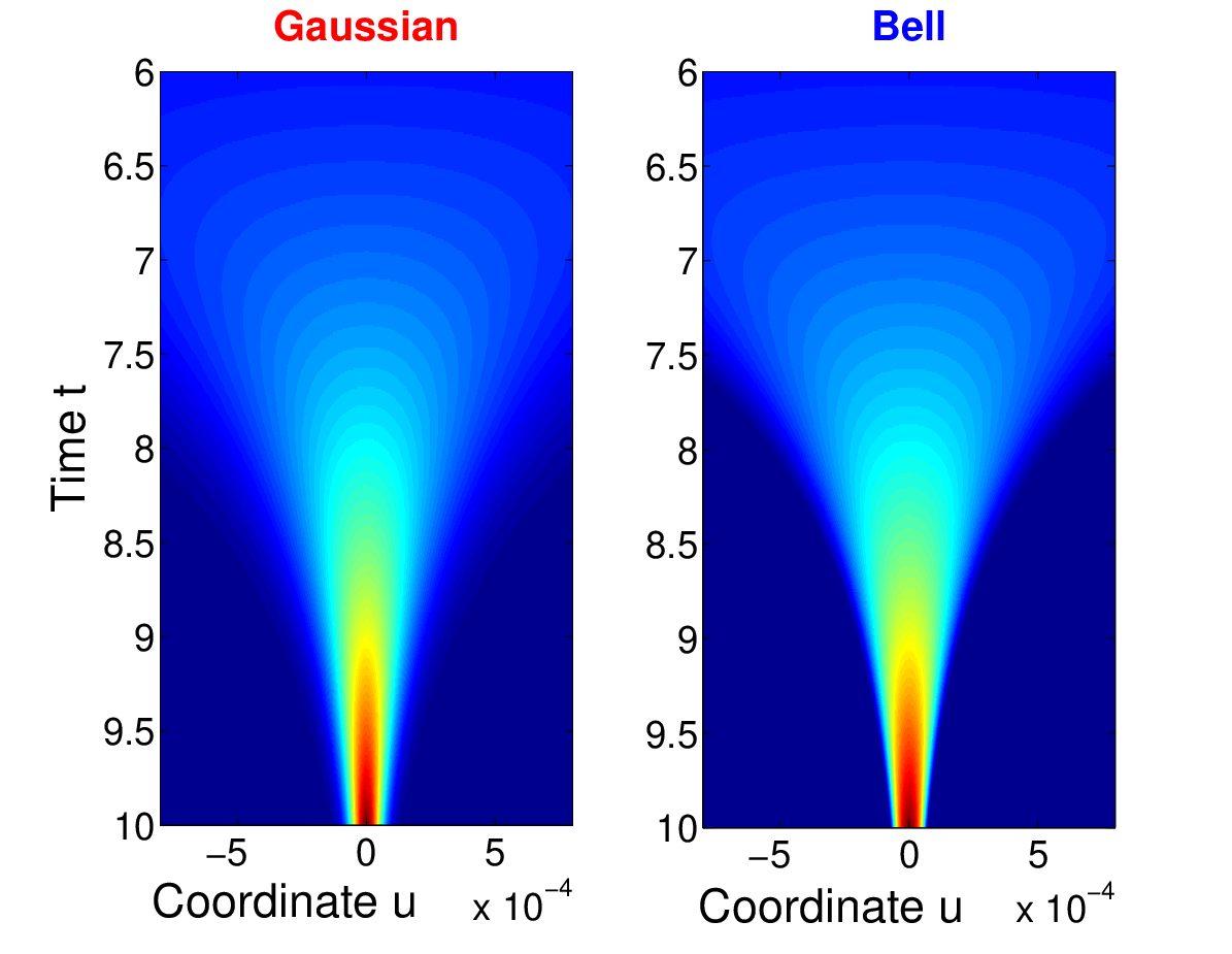
The (u,v)(u,v) phase space remains the simplest configuration for numerical tests of the theory. Since one runs into a high computational complexity when analyses the background evolution, we choose (u,v)(u,v) phase space to compare the evolution of a Gaussian function with a specific ϕϵ\phi_{\epsilon}. We best fit the normalized Gaussian function by a function ϕϵ\phi_{\epsilon} in order to compare the background function with the difference between these two waves. Figure 15 shows ϕ⁡(u)\phi(u) and its best fit by ϕϵ​(u)\phi_{\epsilon}(u), obtained for ϵ=ϵ0=1,802425\epsilon=\epsilon_{0}=1,802425. Fig. 16 compares the calculated evolution of ϕ⁡(u)\phi(u) and ϕϵ0\phi_{\epsilon_{0}}. We should see the dispersive component that occurs on the boundaries of the Gaussian evolution. However, appreciating the dispersive behaviour is difficult in a linear scale; we report a comparison between ϕ20B​G\phi^{BG}_{20} and ϕ−ϕϵ0\phi-\phi_{\epsilon_{0}} in Fig. 17 in a semilogarithmic scale. The continuous lines represent the Gaussian background for several time values, while the dashed lines give the difference between the Gaussian and the function with compact support. One can now see without difficulties that the outlines on the boundaries are well overlapped, so the long time evolution of a Gaussian background, that is, the dispersive tail of a function not belonging to Φ+\Phi_{+}, can be approximated to the rest between the function we are studying and an appropriately chosen function ϕϵ\phi_{\epsilon}.

Refer to caption
Figure 15: (Color online) Fit of the Gaussian function ϕ⁡(u)=e−u22π4\phi(u)=\frac{e^{-\frac{u^{2}}{2}}}{\sqrt[4]{\pi}} by the function ϕϵ0​(u)\phi_{\epsilon_{0}}(u) (ϵ0=1.802425\epsilon_{0}=1.802425).
Refer to caption
Figure 16: (Color online) Comparison of the Gaussian evolution ϕ⁡(u,t)\phi(u,t) with ϕϵ0​(u,t)\phi_{\epsilon_{0}}(u,t). ϕϵ0​(u,t)\phi_{\epsilon_{0}}(u,t) focalizes without any loss or dispersion of energy, while the Gaussian presents a dispersive background (see lso Fig. 17).
Refer to caption
Figure 17: (Color online) We want to analyze if a region where
ϕNB​G​(u,t)≃ϕ⁡(u,t)−ϕϵ0​(u,t)\phi_{N}^{BG}(u,t)\simeq\phi(u,t)-\phi_{\epsilon_{0}}(u,t) exists. A comparison between ϕ20B​G​(u,t)\phi_{20}^{BG}(u,t) and ϕ⁡(u,t)−ϕϵ0​(u,t)\phi(u,t)-\phi_{\epsilon_{0}}(u,t) is here reported in semilogarithmic scale: these two wave packets are well overlapped on their borders.
Refer to caption
Figure 18: (Color online) One-dimensional evolution of the Gaussian wave ϕ⁡(x)=e−x22π4\phi(x)=\frac{e^{-\frac{x^{2}}{2}}}{\sqrt[4]{\pi}} under a RHO potential.
Refer to caption
Figure 19: (Color online) Evolution of the wave |ϕ||\phi| with initial condition ϕ⁡(x)=e−x22π4\phi(x)=\frac{e^{-\frac{x^{2}}{2}}}{\sqrt[4]{\pi}}.

We want now complete our analysis by considering the (x,p)−(x,p)-system. By the transformation 𝒰\mathcal{U} we see that ϕ​(x)=[𝒰​ϕ​(u)]​(x)\phi(x)=\left[\mathcal{U}\phi(u)\right](x) is a Gaussian function anyway, because

[𝒰​ϕ​(u)]​(x)=π−14​C~​∫ℝe−u22​ei​S​(x,u)​𝑑u=(γπ)14​e−γ2​x2.\left[\mathcal{U}\phi(u)\right](x)=\pi^{-\frac{1}{4}}\tilde{C}\int_{\mathbb{R}}e^{-\frac{u^{2}}{2}}e^{iS(x,u)}du=\left(\frac{\gamma}{\pi}\right)^{\frac{1}{4}}e^{-\frac{\gamma}{2}x^{2}}.

The focusing dynamics in the (u,v)(u,v) space corresponds to a defocusing propagation in the (x,p)(x,p) space as shown in Fig. 18 and in Fig. 19.

IX Conclusions

We reviewed the basic theorems and the mathematical properties underlying the time-asymmetric formulation of quantum mechanics with specific reference to the reversed harmonic oscillator. We considered the propagation of a wave packet in the reversed harmonic oscillator within the rigged Hilbert space framework. We specifically analysed the evolution of a class of functions with compact support in the (u,v)(u,v) phase space and the evolution of a normalized Gaussian function. For the functions with compact support we discussed the way the dynamics in the (u,v)(u,v) maps into the real (x,p)(x,p) space, and verify that the projections of a wave packet on Gamow states decay exponentially. We studied the mechanism of excitation of the background function for a Gaussian function, that does not belong to Φ+\Phi_{+}. The Gaussian function cannot be expressed as an infinite linear combination of GV, and the results is the excitation of a dispersive wave which does not decay exponentially.

In other words, for a RHO the temporal evolution is dominated by a sum of exponentially decaying states with quantized decay rates. Depending on the function class of the initial conditions, one can also observe the excitation of a non-exponentially decaying component, denoted as the background. These findings may be directly tested in the experiments by a proper shaping of the initial conditions. We believe that our results address some of the known concepts of the RHS approach to the dynamics of unstable systems in a way that may find direct application in designing tests of time-asymmetric quantum physics, in fields like Bose-Einstein condensation, superconductors and photonics. Gamow vectors may also open novel possibilities in studying nonlinear waves and their reversibility properties from a fundamental point of view.

X Acknowledgments

We acknowledge fruitful discussions with M. C. Braidotti, M. Materassi, P. M. Santini and P. Verrucchi. This publication was made possible through the support of a grant from the John Templeton Foundation (grant number 58277). The opinions expressed in this publication are those of the authors and do not necessarily reflect the views of the John Templeton Foundation.

References

  • [1] A.Bohm, Phys. Rev. A60, 861 (1999).
  • [2] A.Bohm and N. L. Harshman, Lectures Notes in Phys. 504, 179 (1998).
  • [3] A. Bohm, M. Gadella, and G. B. Mainland, Am. J. Phys. 57, 1103 (1989).
  • [4] I. Prigogine, F. Mayné, C. George, and M. D. Haan, Proc. Natl. Acad. Sci. USA 74, 4152 (1977).
  • [5] I. E. Antoniou and I. Prigogine, Physica A 192, 443 (1993).
  • [6] S. Gentilini, M. C. Braidotti, G. Marcucci, E. DelRe, and C. Conti, Phys. Rev. A 92, 023801 (2015a).
  • [7] S. Gentilini, M. C. Braidotti, G. Marcucci, E. DelRe, and C. Conti, Sci. Rep. 5, 15816 (2015b).
  • [8] S. Longhi and S. M. Eaton, Opt. Lett. 41, 1712 (2016).
  • [9] M. Materassi, Entropy 17, 1329 (2015).
  • [10] M. Zanin, D. Papo, P. A. Sousa, E. Menasalvas, A. Nicchi, E. Kubik, and S. Boccaletti, ArXiv e-prints (2016), 1604.08816.
  • [11] D. Calvani, A. Cuccoli, N. I. Gidopoulos, and P. Verrucchi, Open Syst. Inf. Dyn. 20, 1340002 (2013).
  • [12] N. Perra, V. Zlatic, A. Chessa, C. Conti, D. Donato, and G. Caldarelli, EPL 88, 48002 (2009).
  • [13] Y. Y. Liu, J. J. Slotine, and A. L. Barabási, Nature 473, 167 (2011).
  • [14] U. G. Aglietti and P. M. Santini, Phys. Rev. A 89, 022111 (2014).
  • [15] G. Gamow, Z. Phys. 51, 204 (1928a).
  • [16] G. Gamow, Nature 122, 805 (1928b).
  • [17] M. C. Braidotti, S. Gentilini, and C. Conti, ArXiv e-prints (2016), 1601.05796.
  • [18] D. Chruściński, J. Math. Phys. 44, 3718 (2003).
  • [19] D. Chruściński, J. Math. Phys. 45, 841 (2004).
  • [20] C. G. Bollini, O. Civitarese, A. L. D. Paoli, and M. Rocca, J. Math. Phys. 37, 4235 (1996).
  • [21] O. Civitarese and M. Gadella, Phys. Rep. 396, 41 (2004).
  • [22] R. de la Madrid and M. Gadella, Am. J. Phys. 70, 626 (2002).
  • [23] M. Gadella and F. Gomez, Int. J. Theor. Phys 42, 2225 (2003).
  • [24] G. Barton, Ann. Phys. 166, 322 (1986).
  • [25] E. Celeghini, M. Gadella, and M. A. del Olmo, J. Math. Phys. 57, 072105 (2016).
  • [26] A. Gleason, J. Math. and Mech. 6, 885 (1957).
  • [27] M. H. Stone, Ann. of Math. 33, 643 (1932).
  • [28] G. C. Hegerfeldt, Phys. Rev. Lett. 72, 596 (1994).
  • [29] I. Gradshteyn and I. Ryzhik, Table of Integrals, Series and Products (Academic Press, 1965).
  • [30] P. M. Morse and H. Feshbach, Methods of Theoretical Physics (McGraw-Hill, 1953).
  • [31] M. Abramowitz and I. Stegun, Handbook of Mathematical Functions (Dover Publications, 1972).