Combined Top-Down and Bottom-Up Approaches to Performance-guaranteed Integrated Task and Motion Planning of Cooperative Multi-agent Systemsfootnoteinfosupport
Abstract
We propose a hierarchical design framework to automatically synthesize coordination schemes and control policies for cooperative multi-agent systems to fulfill formal performance requirements, by associating a bottom-up reactive motion controller with a top-down mission plan. On one hand, starting from a global mission that is specified as a regular language over all the agents’ mission capabilities, a mission planning layer sits on the top of the proposed framework, decomposing the global mission into local tasks that are in consistency with each agent’s individual capabilities, and compositionally justifying whether the achievement of local tasks implies the satisfaction of the global mission via an assume-guarantee paradigm. On the other hand, bottom-up motion plans associated with each agent are synthesized corresponding to the obtained local missions by composing basic motion primitives, which are verified safe by differential dynamic logic (d), through a Satisfiability Modulo Theories (SMT) solver that searches feasible solutions in face of constraints imposed by local task requirements and the environment description. It is shown that the proposed framework can handle dynamical environments as the motion primitives possess reactive features, making the motion plans adaptive to local environmental changes. Furthermore, on-line mission reconfiguration can be triggered by the motion planning layer once no feasible solutions can be found through the SMT solver. The effectiveness of the overall design framework is validated by an automated warehouse case study.
keywords
Multi-agent systems, formal verification, motion and mission planning, differential dynamical logic, controller synthesis.footnoteinfo]This paper was not presented at any IFAC meeting. Corresponding author R. R. da Silva. Tel. +1-574-631-3736. Fax +1-574-631-4393.
, , ,
support]This work is supported by NSF-CNS-1239222, NSF-EECS-1253488 and NSF-CNS-1446288 capes]The first author would like to appreciate the scholarship support by CAPES/BR, BEX 13242/13-0
1 Introduction
Cooperative multi-agent systems refer to as a class of multi-agent systems in which a number of homogeneous and/or heterogeneous agents collaborating in a distributed manner via wireless communication channels in order to accomplish desirable performance objectives cooperatively. Representing a typical class of cyber-physical systems (CPS), cooperative multi-agent systems has become a powerful analysis and design tool in the interdisciplinary study of control theory and computer science due to the great potential in both academia and industry, ranging from traffic management systems, power grids, robotic teams to smart manufacturing systems, see e.g. [1, 2, 3, 4, 5] and the references therein.
Mission and motion planning are two fundamental problems in the context of cooperative multi-agent systems and have received considerable attention in recent years. To pursue satisfaction of desired performance requirements, planning methods for cooperative multi-agent systems can generally be divided into two categories: bottom-up and top-down approaches. Bottom-up approaches design local control rules and inter-agent coordination mechanisms to fulfill each agent’s individual tasks, while sophisticated collective behavior of cooperative multi-agent systems manages to ensure certain global properties. Such approaches have gained remarkable success in achieving various mission and motion planning purposes, including behavior-based coordination [1], consensus-type motion planning [29] and local high-level tasks [9]. The bottom-up approach scales well but generally lacks formal performance guarantees, except for certain properties like consensus [29], rendezvous [33] or related formation control [34]. In contrary, starting from a global mission, top-down design methods complements bottom-up ones by following a “divide-and-conquer” paradigm, in which the global mission is decomposed into a series of local tasks for each agent based on their individual sensing and actuating capabilities, and accomplishment of the local missions ensures the satisfaction of the global specification via synchronized [13] [14] or partially-synchronized [15][16] multi-agent coordination. Despite the guarantee of achieving complex high-level global mission and motion plans, top-down design methods lack flexibility and scalability in local control policy design due to their requirement for proper abstraction models. Additionally, the planning complexity quickly becomes prohibitively high as the number of partitioned regions and agents increase, which further hampers the applicability of the abstraction based methods in many practical circumstances.
We are therefore motivated to combine both top-down mission planning procedure with bottom-up motion planning techniques to develop a scalable, reactive and correct-by-design approach for cooperative multi-agent systems that accomplishes high-level global tasks in uncertain and dynamic environments. Our basic idea in this paper is illustrated by the design framework shown in Fig. 1.
Given a global mission in the form of regular languages over the mission capabilities of the underlying cooperative multi-agent system, our proposed framework solves the mission planning problem by introducing a learning-based top-down mission decomposition framework [20], which decomposes the global mission into local tasks that are consistent with each agent’s capabilities. Based on the given local tasks, we solve the corresponding integrated task and motion planning problem of the multi-agent systems by extending our previous results of bottom-up compositional design approach called CoSMoP (Composition of Safe Motion Primitives) [21] from single agent to multi-agent circumstances. First, CoSMoP designs a series of motion controllers (primitives) offline that are verified safe by differential dynamic logic (d) [22] to form necessary building blocks of complex maneuvers for each agent. Next, with the learned local task specification and a scenario map, CoSMoP synthesizes the corresponding integrated task and motion plan via appropriate composition of simple motion primitives whose correctness is justified by using the Satisfiability Modular Theories (SMT) solver and by modular incremental verification procedures. The mission and motion planning problem can be solved successfully if the motion planning layer comes up with a set of feasible motion plans for a fair dynamic environment, i.e. the changes in the environment do not lead any agent to a deadlock. However, if it fails to obtain feasible motion plans or an agent gets in a deadlock, feedbacks can be provided to adjust each agent’s mission plan by exploiting necessary coordinations. Our main contributions lie in
- 1.
We apply formal methods to solve both the mission and the motion planning problems of cooperative multi-agent systems, based on which provably correct mission plans are obtained and feasible motion plans are synthesized through correct-by-construction.
- 2.
Our proposed framework shows great improvement of the scalability issues. On one hand, in the top-down mission planning stage, we use assume-guarantee paradigm [23] to compositionally verify the correctness of all the mission plans, mitigating the “state explosion” issues; on the other hand, we synthesize the corresponding motion controllers by using SMT solver and thus finite abstractions of the environment [24] is avoided.
- 3.
Although the given global mission is not necessarily reactive, our proposed framework does provide solutions for both mission and motion plans that are reactive. First, we develop a modification of the learning algorithm [25] such that it can be applied for local mission planning even the agent’s model is not known a priori; secondly, by composing safe motion primitives, the designed motion controller can reactively interact with (possibly) uncertain environment and with other agents. For example, collisions with either obstacles or other agents are avoided.
The remainder of this paper is organized as follows. Previous work related to multi-agent coordination and control are briefly reviewed in Section 2. After introducing necessary preliminaries in Section 3, Section 4 presents the formal statement of our problem, along with a motivating example that are used throughout the rest of the paper. Section 5 solves the top-down problem while Section 6 solves the bottom-up design problem. Section 7 concludes the paper.
2 Related Work
In this paper, we leverage guidance from this relatively broad body of literature to develop a formal framework to solve the mission and motion planning problems of cooperative multi-agent systems. It is worth noting that the proposed framework shows great features of both bottom-up and top-down design methods. Using such a framework, we demonstrate how formal synthesis and verification techniques can facilitate the design of coordination and control protocols for cooperative multi-agent systems.
2.1 Multi-Agent Systems
The increasing interest in improving the expressiveness of mission and/or motion planning specifications draws our attention to specifying desired multi-agent behavior in the form of formal languages, such as regular languages and temporal logics including linear temporal logic (LTL) and computation tree logic (CTL) [10], which provide formal means of specifying high-level performance objectives due to their expressive power. A common two-layered architecture is usually deployed in the synthesis problems of the formal specifications [38][39]. Based on constructing appropriate finite-state abstractions of not only the underlying dynamical system, but the working environment as well, a control strategy [40], usually represented by a finite state automaton, is synthesized for the satisfaction of the high-level specifications by using formal methods, including model checking [10], supervisory control theory [41][42] and reactive synthesis [40]. This synthesis procedure leads to a hierarchical control structure with a discrete planner that is responsible for the high-level, discrete plan and a corresponding low-level continuous controller. Simulations and bisimulation relations are established [10] as a proof that the continuous execution of the low-level controller preserves the correctness of the high-level discrete plans [3][43].
2.2 Bottom-up Synthesis
One of the most highlighted bottom-up methods in literature can be categorized as the behavior-based [1] approaches, which coordinate multiple agents by composing pre-defined behaviors or distributed learning algorithms from artificial intelligence [6]. It turns out, however, that much of this behavior-based work possesses empirical features that leads to a trial-and-error design process, and therefore lacks guarantees of high-level performance objectives. Recent studies [7][8] have accounted for performance verification of behavior-based schemes; nevertheless, the contribution are mainly made to single-agent cases. To accomplish high-level tasks of cooperative multi-agent systems, many attempts have been made in the context of bottom-up design. Filippidis et al. [9] proposed a decentralized control architecture of multi-agent systems to address local linear temporal logic (LTL) [10] specifications while obeying inter-agent communication constraints; however, the agents therein did not impose any constraints on other agents’ behavior. Guo and Dimarogonas [11] considered the synthesis of motion plans associated with each agent to fulfill corresponding local LTL specifications by developing a partially decentralized solution which formed clusters of dependent agents such that all individual tasks can be finished in an orderly manner. To overcome the computational issues, the results were further extended in [12] by involving receding horizon planning techniques.
2.3 Top-down Synthesis
Karimadini and Lin [17] studied task decomposition problems of cooperative multi-agent systems, and necessary and sufficient conditions were derived under which the global tasks can be retrieved by the assigned local specifications in the sense of bisimulation [10]. Task decomposition from a computationally tractable fragment of computation tree logic (CTL) specifications were also investigated by Partovi and Lin [18]. Following a top-down architecture, Kloetzer and Belta [15] solved the multi-agent coordination problem from a global LTL specification, by model checking the composed behavior of all agents in a centralized manner; the results were extended in [19], in which optimality and robustness properties of the synthesized motion plans were taken into consideration. “Trace-closed” regular specifications were investigated in [14][16] to automatically deploy cooperative multi-agent teams. Karaman and Frazzoli [13] addressed the mission planning and routing problems for multiple uninhabited aerial vehicles (UAV), in which the given LTL specifications can be systematically converted a set of constraints suitable to a mixed-integer linear programming (MILP) formulation.
Furthermore, even though powerful model checking tools have been exploited [24][27] to synthesize control protocols for formal specifications, these approaches generate open-loop strategies and cannot handle reactive specifications; furthermore, those synthesis methods which work for reactive control protocols [43] are severely limited by their high computational complexity. To mitigate this problem, Wongpiromsarn et al. [49] employed a receding horizon process where a controller only repeatedly worked out a plan for a short time horizon ahead of the current status. Nevertheless, the proposed results have difficulty handling cooperative tasks for multi-agent systems that involved close inter-agent cooperation.
2.4 Symbolic Motion Planning
Control theory has been widely involved to develop performance-guaranteed solutions of planning problems. The classical reach-avoid planning and point-to-point motion planning algorithms [2][26] aim to steer an intelligent agent from a given initial position to some desirable final configuration while avoiding the collision with any obstacles along the way by utilizing various graph search techniques. Nevertheless, exact solutions to this problem are generally intractable, and various efforts have been devoted to efficiently overcoming the computational burden [27][28]. It turns out that extension of single-agent planning algorithms to multi-agent cases can be non-trivial, whereas many attempts have been made to achieve different multi-agent coordination and control purposes, such as consensus [29][30], flocking [31][32], rendezvous [33] and formation control [34] of multi-agent systems. Fulfillment of these coordination goals is ensured by control theoretical analysis and deductive verification, including Lyapunov stability [29][31] analysis, barrier certificates [35], differential dynamic logic [22], and game theory [36][37]. However, these traditional planning and coordination approaches guarantee the steady-state performance of the underlying multi-agent systems, whereas satisfaction of more complex and temporal specifications is not considered.
2.5 Integrated Task and Motion Planning
Traditionally, the high-level task planner for mobile robots sits on top of the motion planner [44]. The task planner sees the world as abstracted symbols and ignores details in geometric or physical constraints, which may cause infeasibility in the motion planning. Therefore, a recent trend is towards an Integrated Task and Motion Planning (ITMP). Earlier efforts in ITMP, such as Asymov [45] and SMAP [46], were still based on abstractions of the working environment and used a symbolic planner to provide a heuristic guidance to the motion planner. Recent work, such as [47] and [48], introduced a “semantic attachment,” i.e. a predicate that is solved by a motion planner, to the symbolic planner. An overview of the recent developments in the symbolic motion planning can be found in [4], where the task planning problem is reduced to model checking. Since these methods are based on abstracted symbolic models of the environments, it is a common assumption that the working environment is known or static and the robot is the only moving object (or the robot itself carries other movable objects). However, in practice, a robot often shares its workspace with others robots or even humans, and the environment often changes over time in a way that is hard to predict.
3 Preliminaries
In this section, we introduce the basic concepts and notations that are used throughout this paper to describe cooperative multi-agent systems and their desired properties.
3.1 Regular Languages
For a finite set , we let and denote the powerset and the cardinality of , respectively; furthermore, let , and denote the set of finite, non-empty finite and infinite sequences that consist of elements from . A finite sequence composing of elements in , i.e., , is called a word over . The length of a word is denoted by . For two finite words and , let denote the word obtained by concatenating and . A finite word is said to be a prefix of another word , written as , if there exists a word such that .
Given a finite event set , a subset of words in is called a (finite) language over . For a language , the set of all prefixes of words in is said to be the prefix-closure of , denoted by , that is, , where denotes the concatenation of two words and . is said to be prefix-closed if . In practice, we use deterministic finite automata to recognize languages.
Definition 1 (Deterministic Finite Automaton).
A deterministic finite automaton (DFA) is a 5-tuple
where is a finite set of states, is a finite set (alphabet) of events, is an initial state, is a partial transition function and is the set of the marked (accepting) states.
The transition function can be generalized to in the usual manner [50]. The language generated by is defined as ; while stands for the language that is marked by . The language that is accepted by a DFA is called a regular language. We focus our study on regular languages in the sequel.
For a non-empty subset and a word over , we use the “natural projection” to form a word over from by eliminating all the events in that does not belong to . Formally, we have
Definition 2 (Natural Projection).
For a non-empty subset , the natural projection is inductively defined as
The set-valued inverse projection is of defined as .
Given a family of event sets , , with their union , we let denote the natural projection from to . For a finite set of regular languages , , the synchronous product of , denoted by , is defined as follows.
Definition 3 (Synchronous Product).
3.2 Differential Dynamic Logic
The Differential Dynamic Logic verifies a symbolic hybrid system model, and, thus, can assist in verifying and finding symbolic parameters constraints. Most of the time, this turns into an undecidable problem for model checking [22]. Yet, the iteration between the discrete and continuous dynamics is nontrivial and leads to nonlinear parameter constraints and nonlinearities in the dynamics. Hence, the model checking approach must rely on approximations. On the other hand, the uses a deductive verification approach to handling infinite states, it does not rely on finite-state abstractions or approximations, and it can handle those nonlinear constraints.
The hybrid systems are embedded to the d as hybrid programs, a compositional program notation for hybrid systems.
Definition 4 (Hybrid Program).
A hybrid program [22] ( and ) is defined as:
where:
- •
is a state variable and a first-order logic term.
- •
is a first-order formula.
- •
are discrete jumps, i.e. instantaneous assignments of values to state variables.
- •
is a differential equation system that represents the continuous variation in system dynamics. is the time derivative of state variable , and is the evolution domain.
- •
tests a first-order logic at current state.
- •
is a sequential composition, i.e. the hybrid program will start after finishes.
- •
is a nondeterministic choice.
- •
is a nondeterministic repetition, which means that will repeat for finite times.
Thus, we can define the formula, which is a first-order dynamic logic over the reals for hybrid programs.
Definition 5 ( formulas).
A formula [22] ( and ) is defined as:
where:
- •
holds true if is true after all runs of .
- •
holds true if is true after at least one runs of .
uses a compositional verification technique that permits the reduction of a complex hybrid system into several subsystems [22]. This technique divides a system in an equivalent formula , where each can be proven separately. In our approaches we use this technique backwards, we prove a set of formulas , where each one is the motion primitive model, and we use the SMT to compose an equivalent that satisfies a mission task. Therefore, the synthesized hybrid system performance is formally proven.
3.3 Counter Linear Temporal Logic Over Constraint System
We express the specification of an autonomous mobile robot using Counter Linear Temporal Logic Over Constraint System CLTLB() defined in [52]. This language is interpreted over Boolean terms or arithmetic constraints belong to a general constraint system , where is a set of atomic propositions and is a set of arithmetic constraints. Thus, the semantics of a CLTLB() formula is given in terms of interpretations of a finite alphabet on finite traces over a finite sequence of consecutive instants of time with length , meaning that is the interpretation of at instant of time . Moreover, the arithmetic terms of an arithmetic constraint are variables over a domain valuated at instants and, thus, are called arithmetic temporal terms a.t.t.,
Definition 6 (Arithmetic Temporal Term).
A CLTLB() arithmetic temporal term (a.t.t.) is defined as:
where and stands for next and previous operator.
Therefore, a CLTLB() formula is a LTL formula over the a.t.t. defined as below.
Definition 7 (Formula).
A CLTLB() formula (, and ) is defined as,
where,
- •
is a atomic proposition, and is a relation over the a.t.t. such as, for this work, we limit it to linear equalities or inequalities, i.e. , where and .
- •
, , and stands for usual next, previous, until and since operators on finite traces, respectively.
Based on this grammar, it can also use others common abbreviations, including:
- •
Standard boolean, such as , , and .
- •
that stands for , and it means that eventually holds before the last instant (included).
- •
that stands for , and it means that always holds until the last instant.
- •
that stands for , where on finite trace is only at last instant. Thus, it means that is true at the last instant of the sequence .
A CLTLB() formula is verified in a Bounded Satisfiability Checking (BSC) [53]. Hence, it is interpreted on a finite sequence with length . Therefore, means that holds true in the sequence at instant ().
Definition 8 (Semantics).
The semantics of a CLTLB() formula at an instant is as follow:
- •
.
- •
.
- •
.
- •
.
- •
.
- •
.
- •
.
- •
.
4 Problem formulation
4.1 A Motivating Example
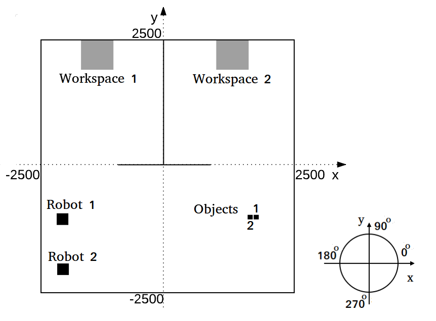
As a motivating example, let us consider a cooperative MRS with robots in an automated warehouse as shown in Fig. 2. The global mission is to deploy the robots to move newly arrived goods to respectively designated workspaces. Additionally, the robots are Pioneer P3-DX robots11 1 http://www.mobilerobots.com/ResearchRobots/PioneerP3DX.aspx, retrieved 05-18-2016. which is fully programmable and includes a dedicated motion controller with encoder feedback. Moreover, this robot can be simulated with the MobileSim22 2 http://www.mobilerobots.com/Software/MobileSim.aspx, retrieved 05-18-2016.. This application permits to simulate all current and legacy models of MobileRobots/ActivMedia mobile robots such as Pioneer 3 DX and AT. Moreover, full source code is available under the GPL for understanding the simulation implementation, customizing and improving it.
Furthermore, the Pioneer P3-DX robot has a software developing kit called Pioneer SDK33 3 http://www.mobilerobots.com/Software.aspx, retrieved 05-18-2016. which allows developing its control system in custom C++ applications with third-part libraries such as an SMT solver. Particularly, the examples presented in this paper are implemented using two libraries from this kit: ARIA44 4 http://www.mobilerobots.com/Software/ARIA.aspx, retrieved 05-18-2016. and ARNL55 5 http://www.mobilerobots.com/Software/NavigationSoftware.aspx, retrieved 05-18-2016.. The ARIA brings an interface to control and to receive data from MobileSim accessible via a TCP port and is the foundation for all other software libraries in the SDK such as the ARNL. Moreover, the ARNL Navigation library66 6 http://www.mobilerobots.com/Software/NavigationSoftware.aspx, retrieved 05-18-2016. provides a MobileRobots’ proprietary navigation technology that is reliable, high quality and highly configurable and implement an intelligent navigation and positioning capabilities to this robot. Different localization (positioning) methods are available for various sensors such as LIDAR, Sonar, and GPS. Furthermore, commands can be sent to a custom application implementing those libraries by using a graphical interface called MobileEye77 7 http://www.mobilerobots.com/Software/MobileEyes.aspx, retrieved 05-18-2016. which shows the sensor readings and trajectories. Hence, each robot dynamics is simulated in MobileSim, and each controller is implemented in a C++ custom application that both run on Linux Computers. These computers are connected through Ethernet, and each robot controller connects via a TCP port to MobileSim and other robot neighbors. Therefore, all examples presented in this paper can be implemented in a custom C++ application using both the Pioneer SDK and the SMT solver (e.g. Z3).
This article illustrates the control system design using a simple example shown in the Fig. 2. Denote , we initially assume and all the robots , have the identical communication, localization and actuation capabilities. Our design framework can be extended to involve robots with different capabilities and other scenarios like search and rescue as well, and it will be presented an example with .
This robot team may share its workspace with humans and deal with unexpected obstacles such as a box that falls from a shelf. Some goods must be moved first before the others can be picked up, some maybe quite heavy and require two robots to move; therefore coordination between robots is needed for the safety as well as the accomplishment of the global task.
4.2 Cooperative Mission Planning Problem
Motivated by the fact that the accomplishment of missions among cooperative multi-agent systems shows strong event-driven features, we characterize the mission planning problem within the discrete-event system (DES) formalism [50]. For a cooperative multi-agent system that consists of interacting agents, let denote the set of missions that can be accomplished by the -th agent, . In practical mission planning problems, events in shall represent the sensing, and actuating capabilities of the underlying agent; and execution of an event indicates that the -th agent may accomplish a certain action. The “global” missions are then captured by the union of mission capabilities of all agents, i.e., . For the clarity of presentation, we assume that the mission transition diagram of each agent is given by a prefix-closed regular language .
The mission alphabet , of the motivating example are listed in Table 1 with an explanation of the corresponding service and mission capabilities.
| Event | Explanation |
|---|---|
| Robot picks up object . | |
| Robot drops off at workspace . | |
| Robot returns to its original position. | |
| is moved away | |
Inter-agent communication for the purpose of multi-agent coordination are considered at this point by imposing extra constraints on events shared by more than one agent. For each agent , , we associate a pair of request and response communication events, respectively as follows:
and
where a request event indicates that the underlying agent sends a message through the communication channel, and a response event indicates a message reception. In the warehouse example, is a communication event where denotes a request event that some robot wants the to be moved away. denotes a response event that some robot moves away and notifies the robot who made the request.
The team task is given in the form of a prefix-closed regular language associated with its DFA representation. The design objective of the mission planning is to decompose the global mission into local tasks , , such that , i.e., . That is, the collective team behavior should not exceed the global mission. In summary, the top-down design objective is to solve the following distributed cooperative tasking problem.
Problem 4.1 (Cooperative Mission Planning).
Given a non-empty and prefix-closed global mission and , local mission sets of each robot, systematically find locally feasible mission plans for each robot such that .
The team mission for the automated warehouse example is as shown in Fig. 3. All the horizontal events of the same column and all the vertical events of the same row are identical.
4.3 Integrated task and motion planning
Given the local mission plan for each robot , the underlying integrated task and motion planning problem is to implement the task with safety guarantees.
The description of the scenario environment is essential for the integrated task and motion planning problem. Hence, we first define the scene description which provides the basic information of the robot workspace. Since the Pioneer P3-DX robot is a ground vehicle, its workspace can be specified in 2D.
Definition 9 (Scene Description).
Scene description is a tuple :
- •
Obstacles : a set of polygon obstacles described by line segments specified by two points , where ;
- •
Agents : a set of robots which are represented as a square described by their length and their initial state .
- •
Objects : a set of movable objects which are specified as an square described by their length and their initial state , where .
The states variables of the robots and objects are defined over instants of time indicating the execution ending events of the primitives. Those instants of time are defined by , as defined in Sec. 3.3, and it denotes the time instant that the th action has been taken. Thus, we denote the robot state variables as which represents the robot pose, where specify the position in and is angle in degrees. Hence, a CLTLB() formula , for example, means that the robot state variable value at instant should be always equal to the value of at . Correspondingly, the object state variables are expressed as which describes its 2D position , and and are Boolean propositions that holds true when the robot is carrying this object, and holds true when another robot is taking this object away from its initial position. Next, we define a scene description for the particular scenario as shown in Fig. 2
Example 4.2.
The Fig. 2 a scene of an automated warehouse which two robots must drop two objects off in two different workspaces. Note that the origin is at the center of the workspace. The robots are represented as black filled squares with side length which start at bottom left of this warehouse, i.e. . The objects are initially at bottom right of the warehouse and are depicted as black filled square too with side length , i.e. . The obstacles refers to the four boundary lines that limits the scene which are formally specified as a set of line segments and to the two walls that separate the workspaces shown as gray squares, i.e. . The challenge in this scene is that the objects are adjacent to each other; therefore, a plan that includes both robots picking them up at same time requires a cooperative behavior.∎
Problem 4.3 (Reactive Motion Planning).
Given a team of robots and their mission plans , the scene description , and the trace length for each robot , solve an integrated task and motion planning problem by splitting it into three steps. First, design a set of safe motion primitives for each robot and respective motion primitives specification . A safe motion primitive for the robot is a certified controller which guarantees a safety property and can be reactive changing its control values based on actual sensor readings. The motion primitives specification is a CLTLB() formula which specifies the safe motion primitives by defining constraints for the state variables and the given scene description . Second, for each robot , check if the mission plans are satisfiable for the scene in a fair environment using the controllers for each robot . An environment is fair when all moving and static obstacles that are not in the scene description do not lead any robot to a deadlock. Third, for all plans that are satisfiable, find a trace with length for each robot , where at instant . is a sequence of assigned values for robot states such as are the values at instant . is a sequence of assigned primitives such as is a motion primitive at instant that defines to robot what primitive to take at to go to .
Note that we are restricted to take at most actions in each mission plan and robot . The motion controller refers to actions that a robot can execute, such as moving to some place, picking up objects and so on. Such actions are designed underlying low-level control law from which the generated trajectories are guaranteed to be safe considering both the environment geometrics and kinematics.
5 Top-down design and Task Decomposition
This section concerns with Problem 1 and derives a systematical approach to decompose the global task into feasible local tasks. In our previous work [54], a counterexample-guided and learning-based assume-guarantee synthesis framework was proposed. We adopt this framework in the top-down layer in Fig. 1 to automatically learn the local missions .
Fig. 4 shows the flowchart of the automatic task decomposition and coordination framework that solves Problem 1 by executing the following steps iteratively.
- •
Task decomposition Obtain a prefix-closed and feasible local mission for robot from the global mission .
- •
Compositional verification We determine whether or not the collective behaviors of each agent can satisfy the global mission by deploying a compositional verification [54] procedure with each behavior module being a component DFA that recognizes . In particular, to mitigate the computational complexity, we adopt an assume-guarantee paradigm for the compositional verification and modify algorithm [25] to automatically learn appropriate assumptions for each agent.
- •
Counterexample-guided synthesis If the local missions fail to satisfy the global specification jointly, the compositional verification returns a counterexample indicating that all the share a same illegal trace that violates the global mission. We present such counterexample to re-synthesize the local missions.
We illustrate the task decomposition using the automated warehouse example in Section II. In the framework shown in Fig. 4, local missions , are obtained by as shown in Fig. 5, where stands for the natural projection [50] from the global mission set to the mission set of the -th robot, . Under the assumption that the global mission is feasible, i.e., , we point out that every mission specification is locally feasible.
Given a series of feasible local missions for , the next question is whether or not the fulfillment of all local missions can imply the satisfaction of the global one. This question is addressed by deploying a compositional verification procedure [54]. Specifically, by setting as the -th behavior module, the compositional verification justifies whether or not using an assume-guarantee scheme. In the assume-guarantee paradigm for compositional verification, a formula to be checked is a triple , where is a module component, is a property and is an assumption about ’s environment, which can also be represented by a DFA. The formula is true if whenever is part of a system satisfying , then the system must also guarantee the property , i.e., , implies that . For the warehouse example, we check the achievement of by following an asymmetric proof rule.
| 1 | |
|---|---|
| 2 | |
Here denotes an assumption about the environment (including mission plan performed by robot ) in which robot is placed. To automatically generate appropriate assumptions, we consider the learning algorithm proposed in [25]. creates a series of observation tables to incrementally record and maintain the information whether traces in belong to . An observation table is a three-tuple consisting of: a non-empty finite set of prefix-closed traces, a non-empty finite set of suffix-closed traces and a Boolean function, called a , . Once the observation table is closed and consistent [25], a candidate DFA over the alphabet is constructed. If , where is the generated language of [50], then the oracle returns “True” with the current DFA ; otherwise, a counterexample is generated by the oracle. then adds all its prefixes to , which reflects the difference in next conjecture by splitting states in , and iterates the aforementioned process to update with respect to . For the purpose of compositional verification, we modify by using the following family of dynamical membership queries.
| (2) |
where is a deterministic finite automaton that generates and accepts . In the warehouse example, an appropriate assumption for robot is depicted in Fig. 6.
Next, we check whether or not , which turns out to be true in the warehouse example. Thus one can conclude that the joint behavior of the two robots can cooperatively accomplish the global mission.
Remark 5.1.
In case where , the compositional verification procedure essentially justifies the separability of the global mission [51] with respect to , , i.e., ; while the assume-guarantee paradigm avoids “state explosion” in the compositional verification. In case is not separable, the compositional verification fails and returns a counterexample indicating a violation of the global mission. We present such counterexample to re-synthesize the local missions by resetting . It has been shown in [55] that, under the assumption that the independence relation induced by the distribution is transitive, can always possess a non-empty separable sublanguage.
6 Bottom-up Design and Integrated Task and Motion Planning
This section solves the Problem 2 and illustrates it through the warehouse example. This section is based on extensions of our previous work [21] to multi-robot coordinations. In [21], a bottom-up approach called CoSMoP (Composition of Safe Motion Primitives) was proposed. It features a two layer hierarchical motion planning as shown in Fig. 7 for each robot. The global layer synthesizes an integrated task and motion plan for the local layer considering only geometric constraints from a given scene description . If this layer finds a satisfiable plan, the motion supervisor in the local layer implements a designed sequence of controller executions satisfying all kinematic and geometric constraints.

CoSMoP solves Problem 2 in three stages. First, it designs offline a set of safe motion primitives for each robot to provide necessary maneuvers to complete a given task. We omit the index from now on because the controllers are identical for all robots in this paper. Second, for each primitive , it designs offline the corresponding specification in CLTLB() formula to the global layer, where is a specification to be satisfied and the conjunction the specifications for all primitives is denominated motion primitives specification , i.e. . Finally, it composes a sequence of safe motion primitives to ensure the local mission and the motion primitives specification . It is solved automatically and distributively for each robot . The following subsections will formally describe each of these steps illustrating with the Example 4.2.
6.1 Design of Safe Motion Primitives
In the warehouse scenario, each robot requires five primitives such that , where GoTo, PickUp, DropOff, ?ObjAway (i.e. request to take an object away), !ObjAway (i.e. respond that an object is taken away).
6.1.1 GoTo
The controller GoTo synthesizes trajectories towards a goal position based on the actual sensors readings to avoid static and moving obstacles. It can guarantee safety concerning collisions not only for the obstacles described in the scene description but for other obstacles such as non-controlled agents (e.g. humans or felt down boxes) and neighbors robots. Therefore, this controller allows local and distributed trajectory synthesis that satisfies safety properties for multi-agent systems.
The Pioneer P3-DX robot implements an embedded controller for the translational and the angular velocities based on the maximum acceleration , deceleration and angular velocity . Hence, the GoTo controller is responsible for finding and realizable in a cycle time that specify a motion to drive the robot forward reducing the time to destination and guaranteeing the passive safe property [56]. This property means that the vehicle will never actively collide, i.e. the collision can only occur when the vehicle is stopped, and the obstacle runs into it. This property does not use the ICC (Inevitable Collision State) concept [57] because the limited range of the sensors readings and the limited knowledge assumed about the moving obstacles kinematics give limited awareness of the environment. Therefore, the controller cannot ensure that it will always find a collision-free motion.
The robots motion is a sequence of arcs in two-dimensional space such that the translational velocity is non-negative, the absolute value of the angular velocity is and the maximum cycle time is . An arc is specified by the translational and angular velocities and cycle time , i.e. . The domain of the arcs is . Several types of robots can realize a motion , such as differential drive, Ackermann drive, single wheel drive, synchro drive, or omni drive robots [58]. Therefore, the trajectory realized by the Pioneer P3-DX is a motion . Furthermore, this motion can be modeled in d to find a set such that ensures the passive safety property.
The primitive implements an extended Dynamic Window Approach [59] (DWA) algorithm to avoid not only static obstacles but the ones that can be moving at a velocity up to . We extend a path planning algorithm implemented in the ARNL library that synthesizes and executes trajectories to a given destination based on a map that can be generated using Mapper388 8 http://www.mobilerobots.com/Software/Mapper3.aspx, retrieved 05-18-2016.. This algorithm synthesizes two trajectories: global and local trajectories. The global trajectory is a roadmap generated by an A* that considers only the static obstacles represented on the map, such as walls. The local trajectory is the trajectory implemented using a DWA algorithm that drives along the global trajectory while avoiding unmapped obstacles such as the other robots.
In summary, the DWA control searches for an arc at every cycle time that maximizes towards the target while avoiding a collision with obstacles that can be moving up to velocity . It is organized in two steps. (i) First it searches for the dynamic window that is a range of admissible pair that results in safe trajectories that the robot can realize in a short time frame such as . A safe trajectory is the one that does not lead to a collision with an obstacle detected by the sensors readings. (ii) Then, it finds that chooses a pair that maximizes the progress towards the closest next destination in the global trajectory.
Such control system must satisfy a safety property after all its executions assuming that it starts in a state that satisfies and arrives in a state that satisfies . The Fig. 8 shows a representation of this model in a transition system. Since depends on the environment dynamics because it must be guaranteed after all executions of , we call this property tight coupled. Furthermore, this formula is specified as a passive safety property defined in [60] as,
where are the closest position of the robot and the nearest obstacle, respectively.
The added feature in the extended DWA is that the robot will take a circular trajectory if the condition , as defined below, holds true; otherwise, it will stop. This condition is a first-order logic formula which constraints the robot state variables considering the delay caused by the cycle time.
Finally, the controller is verified for .
Theorem 10.
[60] If the controller GoTo starts in a state that satisfies , it will always satisfies it.
where constraint only the parameters (e.g. , , and ) and does not depend on any environment state, is the hybrid program presented in Model 1 in [60], and it models the execution of the controller GoTo in d for a dynamic environment with moving obstacles with maximum velocity .
To guarantee passive safety, we solve the condition and add the velocity variation with maximum acceleration for maximum cycle time (i.e. ) to find the maximum value for the translational velocity setpoint .
Corollary 6.1.
A circular trajectory is safe if the controller setpoint such as ,
PROOF.
From Model 1 in [60], if a translational velocity satisfies the condition for given position and parameters, then the acceleration can be any value between and . Since we assume that the minimum velocity for the robot is zero (), then the condition only constraint the maximum of velocity . However, the maximum translational velocity is the velocity maximum that could be reached in the next sampling time. Thus, if holds true, the robot is allowed to accelerate up to , and the maximum velocity is . Otherwise, the robot must brake, and the maximum velocity is .
6.1.2 Pick Up and Leave
We assume that the objects in the warehouse will be picked up and dropped off by robot’s gripper with a fixed robot pose, as presented in [21]. Hence, it must satisfy a property that ensures that the robot is carrying the object after picking it up assuming that it starts in a state that satisfies that guarantee that the robot is in front of the object. In contrast to the GoTo primitive, this primitive is non-tight coupled controller, meaning that should be guaranteed only in the last state after finite executions . The transition system of this controller is shown in Fig. 9. Therefore, these properties do not depend on the robot dynamics and do not need to be verified in d.
6.1.3 Request and Response to Move Object Away
We assume that the robot is stopped temporarily during the communication events. For the request controller , the robot sends a request to have object moved away and waits until it receives a response message. It then continues the next planned action. The response controller means that the robot will send a message to indicate that the object is being moved. These primitives do not require tightly coupled safety property either, so they are not verified in d.
6.2 Design of the Motion Primitives Specification
From the local layer, we need to specify constraints for each designed controller to the global layer. The conjunction of these constraints is called the motion primitive specification and is shown in the Fig. 7 as one of the inputs for the constraint generator. These constraints are formulas in CLTLB() which allow the global layer to omit the kinematic constraints implemented in the controller so only geometric constraints will be considered. The CLTLB() is an extension of linear temporal logic (LTL) for bounded satisfiability checking (BSC) [53] that the models consist of temporal logic rather than transition systems; thus, the problem encoding can be more compact and elegant. Moreover, it is possible to encode CLTLB() into satisfiability modulo theories (SMT) [52] and use SMT solver to check if the specification can be satisfied.
The formulas are specifications which constrains the states and generated in the robot global layer. A state is assigned values for states variables in the environment at instant and the primitive taken between instants and . Hence, this state is defined as , where , and are sequences of assigned values to robot and object states variables at each instant and assigned motion primitive to take between instants and , respectively. Each must ensure that, for any plan for the robot , the following two conditions hold:
- •
For each , is satisfiable for at least one trajectory between and .
- •
For each , and .
The specifications , and are safety properties in d formulas for the primitive assigned at instant (i.e. ). If those conditions hold true, any plan generated in the global layer that satisfies will guarantee the safety properties. Furthermore, the reachable states after any execution of the controller assigned in will be constraint to satisfies initially , after any execution of and it will satisfy before execute the next assigned controller .
Theorem 11.
If a plan with size satisfies (i.e. ) for a given scene description and the safe motion primitives are safe (i.e. is valid), then this plan is also safe (i.e. ).
PROOF.
The transition system of the plan is represented in the figure below.
Since the controllers can be reactive, we assume that they will execute finite times until reaching the goal state that satisfies . Thus, the safety property must be ensured in the intermediate states. Let is the d hybrid program that models , thus, the transition system can be modeled using d formulas as in the figure below.
The constraints defined in the specifications can be modeled in the d hybrid program using the operator . Therefore, the d formula of resulting plan is,
By applying the rules and [22], we find the equivalent formula,
| (3) | ||||
We know that is valid, it means that any initial state that satisfies can execute any finite times modeled as hybrid program that it will lead to a state that is safe, i.e. satisfies . Hence, it is sufficient that the global layer find a plan that satisfies to satisfy the Eq.3 and, consequently, the safety property of all motion primitives for the robot in the scene description .
In the next subsections, the specifications for each safe motion primitive are designed.
6.2.1 GoTo
The controller requires a tightly coupled safety property; thus we need to ensure that is satisfiable for at least one trajectory between any planned and states. However, we assume and here because these properties do not depend on the geometry or dynamics in the environment, considering that all parameters are correctly assigned (e.g. ). These assumptions leave the primitive free to drive the robot to the positions required by the other primitives. Note that is also an invariant property, as shown in Theorem 10, so we can use it to reason the existence of a safe trajectory. The global layer omits dynamic constraints; as a result, it is assumed that the minimum robot velocity is zero (), and the obstacles are static (). From the Corollary 2.1 in [21], the Go To specification in CLTLB() should guarantee that there exists a trajectory that the robot fits in between the initial and goal state using a linear arithmetic relation.
Theorem 12.
There exists a trajectory between and which satisfies the controller safety property , if there exists a sequence of waypoints which the robot starts at the initial state and reaches a goal state that satisfies the following two conditions. First, all pairs of states and in this sequence (i.e. ) are in region below, above, left or right of all objects line segments . Second, the environment is fair, meaning that obstacles not in the scene description do not lead the robot executing the primitive GoTo (i.e. ) to a deadlock. In this definition, it is used the a.t.t. operator as shorthands for implications of (e.g. ), where means no implication.
PROOF.
First, since it is a fair environment, then a trajectory that is safe for static obstacles is enough to ensure the existence a safe trajectory for a dynamic environment with moving obstacles. Second, the robot states and constrained in one of the regions below, above, left or right of a line segment , as shown in the Fig. 10, ensure the existence of a safe trajectory. This safe trajectory may be straight line trajectory that guarantees by using the Corollary 2.1 in [21]. Moreover, those regions intersect with each other, causing the existence of waypoints which is inside of more than one of these areas. Hence, it allows finding intermediate trajectories to link two states which are not in the same region. Therefore, if a sequence of waypoints is found, there is a composition of two or more straight trajectories which leads a initial state to a goal state . Furthermore, those trajectories and their composition satisfy the safety property when executing the primitive GoTo.


Therefore, any pair of states and for robot should satisfy the following specification,
, where
- •
;
- •
;
- •
;
- •
;
- •
;
- •
;
- •
;
- •
;
- •
;
- •
;
- •
;
- •
;
- •
;
- •
;
- •
;
- •
;
- •
;
- •
;
- •
;
- •
;
- •
;
- •
;
- •
;
- •
;
- •
;
- •
;
- •
the operator returns if holds true, otherwise .
Note that if a constraint , , or holds true, then the states and are in the regions below, above, left or right, respectively.
And similarly we have to avoid colliding into objects that are not being carried (i.e. ) and not away (i.e. ). Thus, the initial and goal states should be to the left, right, below or above of all objects (i.e. , , , , where ),
Finally, the robot should’t change any object state (i.e. and ) when executing , so, we have,
6.2.2 PickUp and DropOff
We assume that the robot can only pick up the object when . Hence, to pick an object up, the robot cannot be carrying any object (i.e. ) and will carry the object (i.e. ). Also, the robot initial and goal states will not change (i.e. ) and it will be posing in front of object (i.e. ),
Accordingly, we drop the object off at the same angle. Thus, the robot should be carrying the object (i.e. ) and, then, not (i.e. ). Moreover, the robot will not change its the initial and final states (i.e. ) and the object will be left next to it at (i.e. ). However, we cannot leave the object over other objects. Therefore, the next object position should be to the left, right, below or above of all other objects (i.e. , , , , where ),
Similarly, neither over an obstacle. Hence the object should be left to the left, right, below or above of all obstacles ,
, where
- •
;
- •
;
- •
;
- •
;
- •
;
- •
;
- •
;
- •
;
- •
;
- •
;
- •
;
- •
;
Therefore,
Finally, we allow changing the object position only if the robot leaves it.
6.2.3 Request and Response to Move Object Away
The abstraction of request controller constraints that the object state must change from to (i.e. ) before continuing the rest of the task. Also the robot is static (i.e. and ) in a position that provide enough space for other robots to pick the requested object up (i.e. robot away from object , ). Thus,
For the response controller , its abstraction also constraints that the robot is static (i.e. and and ). Furthermore, the object must already be picked up (i.e. ) and the robot state must eventually provide enough space for another robot to pick up their objects (i.e. ). Hence,
6.3 Composition of safe motion primitives
The composition of safe motion primitives is implemented in the global layer as shown in the Fig. 7 based on the generated local mission plan . Specifically, we assume that the following are given,
- •
a local mission presented by a DFA;
- •
a scene description ;
- •
a motion primitive specification .
First, we encode as a CLTLB() specification to the SMT solver online. With these encoding, we can check if is satisfiable in the scene description for available safe motion primitives. If yes, we find a roadmap with minimum trace length at the global layer that can be executed at the local layer. If the bottom-up motion planning finds that the is not feasible, it will provide feedback to require and initiate inter-agent coordination in the top-down mission planning, resulting in the re-allocation of the local missions .
6.3.1 Encoding of the local mission plan
We encode each event into a symbol that represents a CLTLB() formula that describes which reactive motion controllers can be executed. For the Example 4.2, the events , , , can be encoded as:
Then we encode the sequential DFA mission plan with nested until operator . For example, in Fig. 5a is encoded in CLTLB() as .
6.3.2 Encoding to SMT solver
The motion primitive specifications for each robot are the conjunctions of the specifications from each single motion primitive. For the Example 4.2, the specification is,
Now we can compose the motion primitives by encoding the local mission plan and the motion primitive specifications to Z3 SMT solver [61]. If the specifications are satisfiable, the SMT solver will output a feasible plan .
Each state variable defined in the CLTL() specifications are encoded as an array of variables in the SMT solver, because Z3 is a decision procedure for the combination of quantifier-free first-order logic with theories for linear arithmetic [61]. For example, a robot state is encoded as an array such that . A object state is encoded as a two dimensional array such that each element is , where and . Further, each motion primitives will be an array such that each element is , where because we do not assign any value at initial state.
The a.t.t. operator can be encoded by adding or subtracting the array index, for instance, at instant . Therefore, a state formula , which is a formula defined as , can be encoded to quantifier-free first-order logic formulas , where is the instant that holds true. For instance, if , then holds true if holds true at instant .
Encoding temporal logic quantifiers to first order logic requires quantifiers and in relation to the time instants. The quantifier can be implemented using for loop. The can be encoded by using an auxiliary variable such as and, then, also encoded using a for loop. Therefore, we can encode CLTLB() quantifiers to Z3, for example,
- •
- •
- •
- •
- •
- •
Finally, let and be a.t.t.’s, the functions and are encoded with SMT function , i.e. and . Now, we can define a task specification in CLTLB() and find an integrated task and motion plan for the scenario in the Example 4.2 as shown below.
Example 6.2.
If we encode the mission plans in Fig. 5 to the scene description in Example 4.2, the local motion plan for robots and will be,
However, the robot plan requires another robot to move the object away. Therefore, the request event must be added to the mission plan . This feedback information will be used in the mission planning level to check the feasibility of the re-allocated mission plans. To establish the inter-robot coordination, we first add a pair of request-response events to the local missions in order to maintain well-posedness of the multi-robot system. The modified specifications, deemed as and , are illustrated in Fig. 11, respectively. Next, we recall the compositional verification procedure stated in Section III to examine whether or not , where , . It turns out that the new missions are satisfiable and the global mission can be accomplished jointly.
Hence, a new plan is generated for that satisfies including a response primitive ,
Note that those plans are safe to moving obstacles including other agents. For example, when the robot is executing the primitive GoTo to go to pose (i.e. ), it may encounter the robot executing GoTo to go to pose (i.e. ). Thus, those robots will generate locally safe circular trajectories to avoid each other with low computation as shown in Fig. 12. Additionally, if the environment is fair, those trajectories will lead them to the goal position. If it is not and our assumption cannot be guaranteed, the robots will always be in the safe state. Hence, we can update the scene description and search for new plans at current state in a receding horizon strategy.

Example 6.3.
Now, we present a scenario that tests the scalability of the proposed approach. The scenario includes a square room with 10 robots and 10 objects as defined above,
The main challenges added in this scenario are: first, we added strings of three objects that should require coordination with more then two robots to pick up them; second, the room is small enough to lead the robots to often cross the way of each other. Hence, we not only add number of robots, which also adds computational effort, but we add complexities in the problem.
The global mission is decomposed in a set of local missions such as,
where,
However, after checking the satisfiability of those local missions, it is found out that the robot requires to move the objects (i.e. ) and (i.e. ), and, similarly, the robot for its respective objects. Likewise, robots requires to move the object , what robots , and also requires for their corresponding objects. Thus, new local missions are generated in coordination layer considering those new assumptions such as for robots and (i.e. ) are:
Equivalently, for robots and (i.e. ):
Furthermore, besides to require to move other objects, the robots and respond a request to robots and , respectively. Hence, these robots local mission (i.e. ) are:
Therefore, the robots and must respond to robots and , and to robots and , accordantly. Consequently, the local missions for these robots (i.e. ) are:
Finally, the robots and must respond to robots and , respectively. Hence, their new local missions (i.e. ) are:
After synthesizing those local missions in the top-down layer and, consequently, the integrated task and motion plans in the global layer of the bottom-up layer, the robots start executing this plan. The Fig. 13 shows the initial instant, when the robots , , and departed from the home position to the designed objects to pick up them. Other robots are requesting them to move the corresponding objects. Subsequently, these robots have responded the moving object away for corresponding requesting robot after these objects being picked up. This communication event is shown in the Fig. 14 in the moment that robot responded to robot and and started to go pick its object up. When a robot crossed another robot way, the robot changes its trajectory reacting to the movement of the other robot every cycle time, as shown in the Fig. 15, 16 and 17. Finally, the Fig. 18 shows that all objects are dropped off to their designed position.


7 Conclusion
In this paper, we proposed a new framework in multi-agent system design by combining the formal top-down task decomposition and bottom up integrated task and motion planning (ITMP) approach CoSMoP in an iterative way.
Our unified framework can decompose the global mission into local missions based on which we synthesize the motion plan with pre-designed motion controllers that are proven to be safe (no active collision). Coordinations are added as necessary based on the feedbacks of CosMoP to guarantee the accomplishment of the global mission. The efficacy of the proposed method is shown in solving a warehouse example.
References
- [1] R. C. Arkin, Behavior-based robotics. MIT press, 1998.
- [2] H. Choset, K. Lynch, S. Hutchinson, G. Kantor, W. Burgard, L. Kavraki, and S. Thrun, Principles of robot motion: theory, algorithms, and implementations. MITPress, Boston, 2005.
- [3] G. E. Fainekos, A. Girard, H. Kress-Gazit, and G. J. Pappas, “Temporal logic motion planning for dynamic robots,” Automatica, vol. 45, no. 2, pp. 343–352, 2009.
- [4] H. Lin, “Mission accomplished: An introduction to formal methods in mobile robot motion planning and control,” Unmanned Systems, vol. 2, no. 02, pp. 201–216, 2014.
- [5] R. R. Negenborn, B. De Schutter, and J. Hellendoorn, “Multi-agent model predictive control for transportation networks: Serial versus parallel schemes,” Engineering Applications of Artificial Intelligence, vol. 21, no. 3, pp. 353–366, 2008.
- [6] J. Ferber, Multi-agent systems: an introduction to distributed artificial intelligence. Addison-Wesley Reading, 1999, vol. 1.
- [7] D. M. Lyons, R. C. Arkin, P. Nirmal, and S. Jiang, “Designing autonomous robot missions with performance guarantees,” in Intelligent Robots and Systems (IROS), 2012 IEEE/RSJ International Conference on. IEEE, 2012, pp. 2583–2590.
- [8] D. M. Lyons, R. C. Arkin, S. Jiang, T.-M. Liu, and P. Nirmal, “Performance verification for behavior-based robot missions,” IEEE Transactions on Robotics, vol. 31, no. 3, pp. 619–636, 2015.
- [9] I. Filippidis, D. V. Dimarogonas, and K. J. Kyriakopoulos, “Decentralized multi-agent control from local ltl specifications,” in 2012 IEEE 51st IEEE Conference on Decision and Control (CDC). IEEE, 2012, pp. 6235–6240.
- [10] C. Baier, J.-P. Katoen, and K. G. Larsen, Principles of model checking. MIT press, 2008.
- [11] M. Guo and D. V. Dimarogonas, “Multi-agent plan reconfiguration under local ltl specifications,” The International Journal of Robotics Research, vol. 34, no. 2, pp. 218–235, 2015.
- [12] J. Tumova and D. V. Dimarogonas, “Multi-agent planning under local ltl specifications and event-based synchronization,” Automatica, vol. 70, pp. 239–248, 2016.
- [13] S. Karaman and E. Frazzoli, “Linear temporal logic vehicle routing with applications to multi-uav mission planning,” International Journal of Robust and Nonlinear Control, vol. 21, no. 12, pp. 1372–1395, 2011.
- [14] Y. Chen, X. C. Ding, A. Stefanescu, and C. Belta, “Formal approach to the deployment of distributed robotic teams,” IEEE Transactions on Robotics, vol. 28, no. 1, pp. 158–171, 2012.
- [15] M. Kloetzer and C. Belta, “Automatic deployment of distributed teams of robots from temporal logic motion specifications,” IEEE Transactions on Robotics, vol. 26, no. 1, pp. 48–61, 2010.
- [16] X. C. Ding, M. Kloetzer, Y. Chen, and C. Belta, “Automatic deployment of robotic teams,” IEEE Robotics & Automation Magazine, vol. 18, no. 3, pp. 75–86, 2011.
- [17] M. Karimadini and H. Lin, “Guaranteed global performance through local coordinations,” Automatica, vol. 47, no. 5, pp. 890–898, 2011.
- [18] A. Partovi and H. Lin, “Assume-guarantee cooperative satisfaction of multi-agent systems,” in 2014 American Control Conference. IEEE, 2014, pp. 2053–2058.
- [19] A. Ulusoy, S. L. Smith, X. C. Ding, C. Belta, and D. Rus, “Optimality and robustness in multi-robot path planning with temporal logic constraints,” The International Journal of Robotics Research, vol. 32, no. 8, pp. 889–911, 2013.
- [20] J. Dai and H. Lin, “Automatic synthesis of cooperative multi-agent systems,” in 53rd IEEE Conference on Decision and Control. IEEE, 2014, pp. 6173–6178.
- [21] R. Rodrigues da Silva, B. Wu, and H. Lin, “Formal design of robot integrated task and motion planning,” in Decision and Control (CDC), 2016 IEEE 55th Annual Conference on, 2016, submitted.
- [22] A. Platzer, Logical analysis of hybrid systems: proving theorems for complex dynamics. Springer Science & Business Media, 2010.
- [23] C. S. Păsăreanu, D. Giannakopoulou, M. G. Bobaru, J. M. Cobleigh, and H. Barringer, “Learning to divide and conquer: applying the l* algorithm to automate assume-guarantee reasoning,” Formal Methods in System Design, vol. 32, no. 3, pp. 175–205, 2008.
- [24] C. Belta, A. Bicchi, M. Egerstedt, E. Frazzoli, E. Klavins, and G. J. Pappas, “Symbolic planning and control of robot motion [grand challenges of robotics],” IEEE Robotics & Automation Magazine, vol. 14, no. 1, pp. 61–70, 2007.
- [25] D. Angluin, “Learning regular sets from queries and counterexamples,” Information and computation, vol. 75, no. 2, pp. 87–106, 1987.
- [26] S. M. LaValle, Planning algorithms. Cambridge university press, 2006.
- [27] A. Bhatia, L. E. Kavraki, and M. Y. Vardi, “Sampling-based motion planning with temporal goals,” in Robotics and Automation (ICRA), 2010 IEEE International Conference on. IEEE, 2010, pp. 2689–2696.
- [28] S. Karaman and E. Frazzoli, “Sampling-based algorithms for optimal motion planning,” The International Journal of Robotics Research, vol. 30, no. 7, pp. 846–894, 2011.
- [29] R. Olfati-Saber and R. M. Murray, “Consensus problems in networks of agents with switching topology and time-delays,” IEEE Transactions on automatic control, vol. 49, no. 9, pp. 1520–1533, 2004.
- [30] W. Ren, “On consensus algorithms for double-integrator dynamics,” Automatic Control, IEEE Transactions on, vol. 53, no. 6, pp. 1503–1509, 2008.
- [31] R. Olfati-Saber, “Flocking for multi-agent dynamic systems: Algorithms and theory,” IEEE Transactions on automatic control, vol. 51, no. 3, pp. 401–420, 2006.
- [32] M. M. Zavlanos, H. G. Tanner, A. Jadbabaie, and G. J. Pappas, “Hybrid control for connectivity preserving flocking,” IEEE Transactions on Automatic Control, vol. 54, no. 12, pp. 2869–2875, 2009.
- [33] D. V. Dimarogonas and K. J. Kyriakopoulos, “On the rendezvous problem for multiple nonholonomic agents,” IEEE Transactions on automatic control, vol. 52, no. 5, pp. 916–922, 2007.
- [34] J. A. Fax and R. M. Murray, “Information flow and cooperative control of vehicle formations,” IEEE transactions on automatic control, vol. 49, no. 9, pp. 1465–1476, 2004.
- [35] D. Panagou, D. M. Stipanović, and P. G. Voulgaris, “Distributed coordination control for multi-robot networks using lyapunov-like barrier functions,” IEEE Transactions on Automatic Control, vol. 61, no. 3, pp. 617–632, 2016.
- [36] E. Semsar-Kazerooni and K. Khorasani, “Multi-agent team cooperation: A game theory approach,” Automatica, vol. 45, no. 10, pp. 2205–2213, 2009.
- [37] J. R. Marden, G. Arslan, and J. S. Shamma, “Cooperative control and potential games,” IEEE Transactions on Systems, Man, and Cybernetics, Part B (Cybernetics), vol. 39, no. 6, pp. 1393–1407, 2009.
- [38] P. Tabuada and G. J. Pappas, “Linear time logic control of discrete-time linear systems,” IEEE Transactions on Automatic Control, vol. 51, no. 12, pp. 1862–1877, 2006.
- [39] M. Kloetzer and C. Belta, “A fully automated framework for control of linear systems from temporal logic specifications,” IEEE Transactions on Automatic Control, vol. 53, no. 1, pp. 287–297, 2008.
- [40] R. Bloem, B. Jobstmann, N. Piterman, A. Pnueli, and Y. Sa‘ar, “Synthesis of reactive (1) designs,” Journal of Computer and System Sciences, vol. 78, no. 3, pp. 911–938, 2012.
- [41] P. J. Ramadge and W. M. Wonham, “Supervisory control of a class of discrete event processes,” SIAM journal on control and optimization, vol. 25, no. 1, pp. 206–230, 1987.
- [42] C. G. Cassandras and S. Lafortune, Introduction to discrete event systems. Springer Science & Business Media, 2009.
- [43] H. Kress-Gazit, G. E. Fainekos, and G. J. Pappas, “Temporal-logic-based reactive mission and motion planning,” IEEE transactions on robotics, vol. 25, no. 6, pp. 1370–1381, 2009.
- [44] J.-C. Latombe, Robot motion planning. Springer Science & Business Media, 2012, vol. 124.
- [45] S. Cambon, F. Gravot, and R. Alami, “Overview of asymov: Integrating motion, manipulation and task planning,” in Intl. Conf. on Automated Planning and Scheduling Doctoral Consortium, 2003.
- [46] E. Plaku and G. D. Hager, “Sampling-based motion and symbolic action planning with geometric and differential constraints,” in Robotics and Automation (ICRA), 2010 IEEE International Conference on. IEEE, 2010, pp. 5002–5008.
- [47] Z. Littlefield, A. Krontiris, A. Kimmel, A. Dobson, R. Shome, and K. E. Bekris, “An extensible software architecture for composing motion and task planners,” in Simulation, Modeling, and Programming for Autonomous Robots. Springer, 2014, pp. 327–339.
- [48] C. Dornhege, P. Eyerich, T. Keller, S. Trüg, M. Brenner, and B. Nebel, “Semantic attachments for domain-independent planning systems,” in Towards Service Robots for Everyday Environments. Springer, 2012, pp. 99–115.
- [49] T. Wongpiromsarn, U. Topcu, and R. M. Murray, “Receding horizon temporal logic planning,” IEEE Transactions on Automatic Control, vol. 57, no. 11, pp. 2817–2830, 2012.
- [50] C. G. Cassandras and S. Lafortune, Introduction to discrete event systems. Springer Science & Business Media, 2008.
- [51] Y. Willner and M. Heymann, “Supervisory control of concurrent discrete-event systems,” International Journal of Control, vol. 54, no. 5, pp. 1143–1169, 1991.
- [52] M. M. Bersani, A. Frigeri, A. Morzenti, M. Pradella, M. Rossi, and P. S. Pietro, “Bounded reachability for temporal logic over constraint systems,” in Temporal Representation and Reasoning (TIME), 2010 17th International Symposium on. IEEE, 2010, pp. 43–50.
- [53] M. Pradella, A. Morzenti, and P. S. Pietro, “Bounded satisfiability checking of metric temporal logic specifications,” ACM Transactions on Software Engineering and Methodology (TOSEM), vol. 22, no. 3, p. 20, 2013.
- [54] J. Dai and H. Lin, “Automatic synthesis of cooperative multi-agent systems,” in Decision and Control (CDC), 2014 IEEE 53rd Annual Conference on, Dec 2014, pp. 6173–6178.
- [55] L. Lin, A. Stefanescu, and R. Su, “On distributed and parameterized supervisor synthesis problems,” Automatic Control, IEEE Transactions on, vol. 61, no. 3, pp. 777–782, 2016.
- [56] K. Macek, D. A. V. Govea, T. Fraichard, and R. Siegwart, “Towards safe vehicle navigation in dynamic urban scenarios,” Automatika, 2009.
- [57] T. Fraichard and H. Asama, “Inevitable collision states—a step towards safer robots?” Advanced Robotics, vol. 18, no. 10, pp. 1001–1024, 2004.
- [58] T. Bräunl, Embedded robotics: mobile robot design and applications with embedded systems. Springer Science & Business Media, 2008.
- [59] D. Fox, W. Burgard, S. Thrun et al., “The dynamic window approach to collision avoidance,” IEEE Robotics & Automation Magazine, vol. 4, no. 1, pp. 23–33, 1997.
- [60] S. Mitsch, K. Ghorbal, and A. Platzer, “On provably safe obstacle avoidance for autonomous robotic ground vehicles.” in Robotics: Science and Systems, 2013.
- [61] L. De Moura and N. Bjørner, “Z3: An efficient SMT solver,” in Tools and Algorithms for the Construction and Analysis of Systems. Springer, 2008, pp. 337–340.