A Geometric Approach to Confidence Regions
and Bands for Functional Parameters

A hyper-ellipse in any Hilbert space can be defined as follows. One needs a center, $m\in{\mathcal{H}}$, axes, $e_{1},e_{2},\cdots$, which are an orthonormal basis for ${\mathcal{H}}$, and a radius for each axis, $r_{1},r_{2},\cdots$. The ellipse is then given by

We note that this definition makes sense even when $r_{j}=0$ or $\infty$. In the former one is saying that the radius in that direction is zero or ‘closed’, while in the latter one is saying that it is infinite or ‘opened’. Since our aim is to construct a confidence region for $\theta$, we will replace the arbitrary axes above with the eigenfunctions $\{v_{j}\}$ and the center with $\hat{\theta}$, to get

This hyper-ellipsoid will be a $1-\alpha$ confidence region for $\theta$ if we find $\{r_{j}\}$ which give

Note that there are actually infinitely many options for $\{r_{j}\}$ but not all of them lead to ‘nice’ regions. We decompose $r_{j}^{2}=N^{-1}\xi c_{j}^{2}$, where $\{c_{j}\}$ are predefined weights (based on $\{\lambda_{j}\}$) for each direction, and $\xi$ is adjusted to achieve proper coverage. We then have

From (2) it follows that the coverage is given by

Therefore, to achieve the desired asymptotic confidence level for a given $\{c_{j}\}$, one can take $\xi$ to be the $1-\alpha$ quantile of a weighted sum of chi-squared random variables. Though the distribution of the weighted sum of chi-squares does not have a closed form expression, fast and efficient numerical approximations exist such as the imhof function in R (Imhof, 1961).

In choosing $\{c_{j}\}$ we suggest two important considerations. The first is that one wants $c_{j}\to 0$ so as to eliminate the effect of later dimensions. In doing so, one is also producing compact regions (Laha and Roghatgi, 1979). Since probability measures over Hilbert spaces are necessarily tight (Billingsley, 1995), meaning they concentrate on compact sets, a region which is not compact is overly large. Conversely, the faster that $c_{j}\to 0$, the larger the mean of $W_{\theta}$, which increases all of the radii. Therefore, it seems desirable to balance these two concerns, choosing $c_{j}$ which go to zero, but not overly fast.

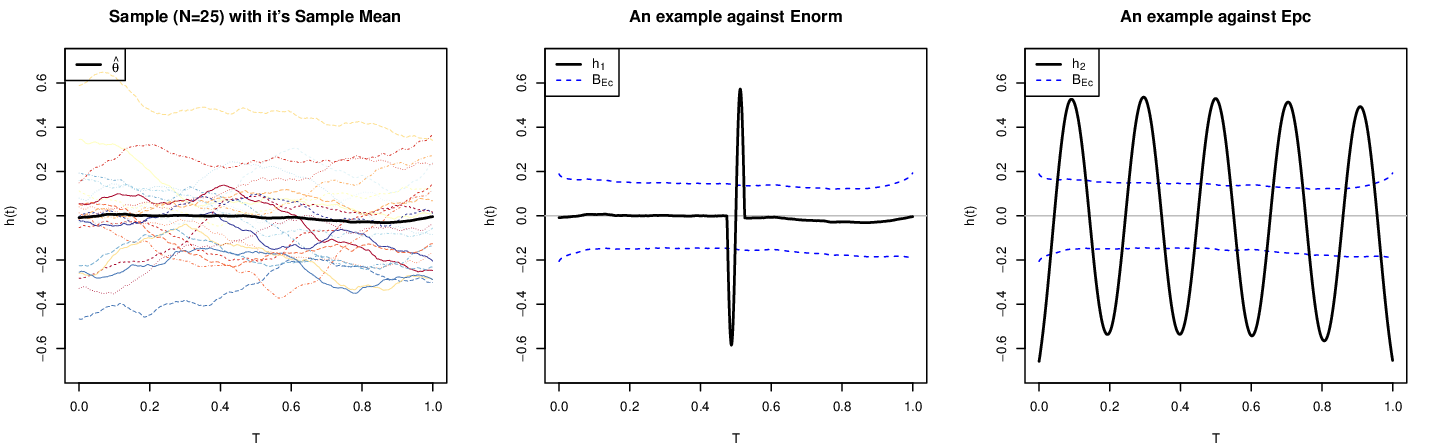
Two popular hypothesis testing frameworks in FDA, the norm approach and PC approach, can be understood as two extreme cases in this framework. The norm approach to test $H_{0}:\theta=\theta_{0}$ uses $N\|\hat{\theta}-\theta_{0}\|^{2}$ as the test statistic. If $H_{0}$ is true, this test statistic, asymptotically, is a weighted sum of $\chi^{2}_{1}$ random variables with weights $\{\lambda_{j}\}$. This corresponds to taking $c_{j}^{2}=1$ for all $j$. The resulting confidence region, which we denote as $E_{norm}$, is a ball in ${\mathcal{H}}$ and provides proper coverage for $\theta$. However, this region is not compact and therefore too large as illustrated in Figure 1. The PC approach to hypothesis testing uses $\sum_{j=1}^{J}{N\langle\hat{\theta}-\theta_{0},v_{j}\rangle^{2}}{\lambda_{j}^{-1}}$ as the test statistic, for some finite $J$. If $H_{0}$ is true, this test statistic follows a $\chi^{2}_{J}$ distribution; therefore, $J$ must be a finite value even when the covariance is known. There are two possible confidence regions induced by this approach. Both regions take $c_{j}^{2}=\lambda_{j}$ for $j\leq J$, but for $j>J$, one could either close them off, $c_{j}=0$, or open them up, $c_{j}=\infty$. The former results in a compact confidence region, but we have ${\mathbb{P}}\left(\theta\in E_{\hat{\theta}}\right)=0$, i.e. zero-coverage even if we make the very artificial assumption that $\theta\in\Span\{v_{1},\dots,v_{J}\}$ since the center of the region $\hat{\theta}$ sits outside $\Span\{v_{1},\dots,v_{J}\}$ almost surely. On the other hand, the opened-up region would achieve proper coverage, but the region is not even bounded, let alone compact.

There exists infinitely many options for proper $\{c_{j}\}$ and how to best choose them is an open question deserving further exploration. In preparing this work, a number of options were initially considered, however, we propose using the following due to 1) its ability to achieve the narrowest average squared width band using tools from Section 2.3 2) excellent empirical performance, and 3) its simplicity:

i.e. the square root of the corresponding eigenvalues. Although $\sum_{j}{\lambda_{j}}{c^{-2}_{j}}\equiv\sum_{j}{\lambda_{j}^{1/2}}<\infty$ is not always guaranteed, this holds for most processes that are smoother than Brownian motion ($\lambda_{j}\approx j^{-2}$), and therefore would hold in most applications. If the process is rough enough such that $\sum_{j}{\lambda_{j}^{1/2}}<\infty$ is not guaranteed, one may use another criteria suggested in the Appendices, namely $c_{j}^{2}=\left(\sum_{i\geq j}\lambda_{i}\right)^{1/2}$, which guarantees both $c_{j}\to 0$ and $\sum_{j}{\lambda_{j}}{c^{-2}_{j}}<\infty$ (Rudin, 1976, p. 80).

Our second form is a slight modification of the previous form, switching from an ellipse to a rectangle. In multivariate statistics a rectangular confidence region is often easier to interpret than an ellipse since it gives clear confidence intervals for each (principal component) coordinate. However, it is often much easier to compute an ellipse since the distributions of quadratic forms are well understood. Regardless, we will show that it can still be easily computed using a nearly closed form expression, up to a function involving the standard normal quantile function.

A hyper-rectangular region can be similarly constructed as:

using the same decomposition $r_{j}^{2}=N^{-1}\xi c_{j}^{2}$. From the KL expansion (2), we want

When we define $z_{j}:=\frac{c_{j}}{\sqrt{\lambda_{j}}}\sqrt{\xi}$, the remaining problem is to find proper $\{z_{j}\}$, or selecting the $\{c_{j}\}$ and finding the proper $\xi$. One may first determine $\{c_{j}\}$ and find the proper $\xi$, or find the proper $\{z_{j}\}$ directly. Again, there exists infinitely many criteria and some examples can be found in the Appendices. Among those, we propose using the following:

where $\Phi^{-1}_{sym}(\cdot)$ is defined as the inverse of $\Phi_{sym}(z):={\mathbb{P}}(|Z|\leq z)$, $Z\stackrel{{\scriptstyle d}}{{=}}{\mathcal{N}}(0,1)$. We denote this rectangular region as $R_{z}$. This criterion produces a region that is close to the one that minimizes $\sup\{\|h-\hat{\theta}\|^{2}:h\in R_{\hat{\theta}}\}$, i.e. the distance between the farthest point of the region from the center, but in a much faster way. It is simple, easy to compute, and shows an excellent empirical performance.

Visualizing a confidence ellipse is challenging even in the finite dimensional setting; it is very difficult once one goes beyond two or three dimensions. In this sense, the rectangular regions are much easier to visualize since one can simply translate them into marginal intervals and examine each coordinate separately (while still achieving simultaneous coverage). It is therefore useful to develop visualization techniques for elliptical regions. One option is to construct bands in the form of an infinite collection of point-wise intervals over the domain of the functions. To make our discussion more concrete, in this section only we assume that ${\mathcal{H}}=L^{2}({\mathcal{D}})$, where ${\mathcal{D}}$ is some compact subset of ${\mathbb{R}}^{d}$. For example, $d=1$ for temporal curves and $d=2$ for spatial surfaces.

A symmetric confidence band in ${\mathcal{H}}$ around $\hat{\theta}$ can be understood as:

The caveat “almost everywhere” here (i.e. except on a set of Lebesgue measure zero) cannot be dropped since we are working with $L^{2}$ functions. The downside of using the above band, however, is that an analytic expression for $r\in{\mathcal{H}}$ usually does not exist. One therefore typically resorts to simulation based methods as in Degras (2011). The band suggested by Degras (2011) takes $c_{\alpha}\hat{\sigma}(t)/\sqrt{N}$ as $r(t)$ where $\hat{\sigma}(t)$ is the estimated standard deviation of $\sqrt{N}\hat{\theta}(t)$. The proper scaling factor $c_{\alpha}$ is then found via parametric bootstrap. We denote this band as $\hat{B}_{s}$, while denoting the one using the true covariance as $B_{s}$.

In traditional multivariate statistics and linear regression, ellipses can be transformed into point-wise intervals and bands using Scheffé’s method which, at its heart, is an application of the Cauchy-Schwarz inequality. This approach cannot be applied as is to our ellipses because they are infinite dimensional. However, a careful modification of Scheffé’s method can be used to generate bands. We now show a $1-\alpha$ ellipsoid confidence region $E_{\hat{\theta}}$ can be transformed into the confidence band $B_{\hat{\theta}}$ such that $E_{\hat{\theta}}\subset B_{\hat{\theta}}$ based on a modification of Scheffé’s method. Defining

then we have the following theorem.

These bands also lead to a convenient metric for choosing an “optimal” sequence $c_{j}$. In particular, we choose the $c_{j}$ which lead to a band with the narrowest average squared width. This is in general a difficult metric to quantify due to $\xi$. However, we can replace $\xi$, which is a quantile of a random variable, by its mean to obtain the following:

Clearly the $\{c_{j}\}$ are unique only up to a constant multiple, however, it is a straightforward calculus exercise to show that one option is to take $c_{j}^{2}=\lambda_{j}^{1/2}$, which is also conceptually very simple. It is also worth noting that this choice does not change with the smoothness of the underlying parameters or the covariance of the estimator; these quantities are implicitly captured by the eigenvalues themselves and thus already built into the $c_{j}$ with this choice. In practice, the coverage of this band will be larger than $1-\alpha$, since $E_{\hat{\theta}}\subset B_{\hat{\theta}}$ and the coverage of $E_{\hat{\theta}}$ is $1-\alpha$. Our simulation studies show that this gap is non-trivial for rougher processes, but narrows substantially for smoother ones. The band formed this way from $E_{c}$ will be denoted as $B_{E_{c}}$.

Our suggested band (7) takes into account the covariance structure of the estimator via the eigenvalues (though the $c_{j}$) and the eigenfunctions. Thus, our band differs from those described in Degras (2011) in that we do not use a constant threshold after taking into account the point-wise variance; our band adjusts locally to the within curve dependence of the estimator. We will illustrate this point further in Section 4 as one of our simulation scenarios will have a dependence structure which changes across the domain. Our band will adjust to this dependence, widening in areas with low within curve dependence and narrowing when this dependence is high.

Lastly, one practical issue arises in finding proper $\xi$ since finding the quantile of weighted sum of $\chi^{2}$ random variables is not straightforward. One may try to invert the approximate CDF, like imhof in R. Alternatively, one can use a gamma approximation by matching the first two moments (Feiveson and Delaney, 1968). Our simulations showed that for typical choices of $\alpha$, such as $0.1,0.05,$ or $0.01$, a gamma approximation works well.

In this subsection we show that the Hausdorff distance, denoted $d_{H}$, between $\hat{E}_{\hat{\theta}}$ and ${E}_{\hat{\theta}}$ can be well controlled. In particular, we will show that this distance converges to zero faster than $N^{-1/2}$. Since this is the rate at which ${E}_{\hat{\theta}}$ shrinks to a point, this is necessary to ensure that $\hat{E}_{\hat{\theta}}$ is actually useful as a proxy for ${E}_{\hat{\theta}}$. We begin by introducing a fairly weak assumption on the distribution of $\hat{C}_{\theta}$. Recall that $C_{\theta}$ is a Hilbert-Schmidt operator (all covariance operators are) in the sense that $\|C_{\theta}\|^{2}_{{\mathcal{S}}}:=\sum_{j=1}^{\infty}\|C_{\theta}(e_{j})\|^{2}_{\mathcal{H}}<\infty$ where $\{e_{j}\}$ is any orthonormal basis of ${\mathcal{H}}$. We denote the vector space of Hilbert-Schmidt operators by ${\mathcal{S}}$, which is also a real separable Hilbert space with inner product $\langle\Psi,\Phi\rangle_{{\mathcal{S}}}:=\sum_{j=1}^{\infty}\langle\Psi(e_{j}),\Phi(e_{j})\rangle_{{\mathcal{H}}}.$ A larger space, ${\mathcal{L}}$, consists of all bounded linear operators with norm $\|\Psi\|_{{\mathcal{L}}}=\sup_{h\in{\mathcal{H}}}\|\Psi(h)\|/\|h\|,$ which is strictly smaller than the ${\mathcal{S}}$ norm, implying ${\mathcal{S}}\subset{\mathcal{L}}$. We now assume that we have a consistent estimate of $C_{\theta}$.

The Hausdorff distance between two subsets $S_{1}$ and $S_{2}$ of ${\mathcal{H}}$ is defined as

We say two regions $S_{1}$ and $S_{2}$ converge to each other if $d_{H}(S_{1},S_{2})$ converges to $0$. Therefore, to achieve convergence of $\hat{E}_{\hat{\theta}}$ to $E_{\hat{\theta}}$ in probability, we need $d_{H}(\hat{E}_{\hat{\theta}},E_{\hat{\theta}})\xrightarrow{P}0$ as $N\to\infty$. To accomplish this, we separate the results for $\rho(\hat{E}_{\hat{\theta}},E_{\hat{\theta}})$ and $\rho({E}_{\hat{\theta}},\hat{E}_{\hat{\theta}})$. Since $\hat{E}_{\hat{\theta}}$ is the “smaller” set, the former is primarily controlled by the distance between the empirical and population level eigenfunctions. The latter is additionally influenced by how large the remaining dimension of $E_{\hat{\theta}}$ is. We define $\{\alpha_{j}\}$ as

Our primary convergence results are given in the following two theorems.

With Theorems 2 and 3 in hand, we can characterize the overall convergence rate for $d_{H}(\hat{E}_{\hat{\theta}},E_{\hat{\theta}})$, but we first need more explicit assumptions on the rates for the eigenvalues, $\lambda_{j}$, and weights, $c_{j}^{2}$.

The first two assumptions are quite common in FDA. One needs to control the rate at which the eigenvalues go to zero as well as the spread of the eigenvalues which influences how well one can estimate the corresponding eigenfunctions, though this can likely be slightly relaxed (Reimherr, 2015). The rate at which $c_{j}^{2}$ decreases to zero also needs to be well controlled, and, in particular, it cannot go to zero much faster than $\lambda_{j}$.

Theorem 4 shows that the squared distance between the ghost region $\hat{E}_{\hat{\theta}}$ and the desired region $E_{\hat{\theta}}$ goes to zero faster than $N^{-1}$, which is the rate at which $E_{\hat{\theta}}$ shrinks to a point. This suggests that $\hat{E}_{\hat{\theta}}$ is a viable proxy for ${E}_{\hat{\theta}}$, even though it has zero coverage.

Interestingly, the rate is better the faster that $c_{j}$ tends to zero, i.e. for larger values of $\gamma$. At first glance, this may suggest that one should actively try and find $c_{j}$ which tend to zero as fast as possible. However, by changing the $c_{j}$ one is changing the confidence region into a potentially less desirable one. In particular, as we will soon see the choice of $c_{j}^{2}=\lambda_{j}^{1/2}$ leads to a suboptimal convergence rate in Theorem 4, but, in some sense, leads to an optimal confidence band and excellent empirical performance. Thus, this may be one of the few instances in statistics where it is not necessarily desirable to have the “fastest” rate of convergence.

We finish this section by stating a Corollary for when $c_{j}^{2}=\hat{\lambda}_{j}^{1/2}$. In this case, we also take into account that the $c_{j}$ are estimated from the data. Note that in Theorem 4 it is assumed that the $c_{j}$ are not random, while in Theorems 2 and 3 the $c_{j}$ can be random or deterministic as long as they are nonincreasing.

We consider the hypothesis testing $H_{0}:\theta=\theta_{0}$ vs. $H_{1}:\theta\neq\theta_{0}$. For a given confidence region $G_{\hat{\theta}}$, the natural testing rule is to reject $H_{0}$ if $\theta_{0}\notin G_{\hat{\theta}}$. For ellipses and rectangles, however, we compare $\theta_{0}$ only in the directions included in the construction of the confidence regions to alleviate the ghosting issue and mimic how the methods would be used in practice. We calculate p-values (detailed in the Appendices) and compare them to $\alpha$. For bands like $B_{s}$ and $B_{E_{c}}$, $H_{0}$ will be rejected if $\theta_{0}$ sits outside the bands at least one evaluation point over the domain.

In this section and in Section 4.2, we take ${\mathcal{H}}=L^{2}[0,1]$ and consider an $iid$ sample $\{X_{i}(t)\}_{i=1}^{N}$, $t\in[0,1]$ from a Gaussian process ${\mathcal{N}}(\theta,C_{\theta})$. To estimate $\theta$ and $C_{\theta}$ (when unknown), we use the standard estimates (Horváth and Kokoszka, 2012) $\hat{\theta}(t)=N^{-1}\sum_{i=1}^{N}X_{i}(t)$ and $\hat{C}_{\theta}(t,s)=(N-1)^{-1}\sum_{i=1}^{N}(X_{i}(t)-\hat{\theta}(t))(X_{i}(s)-\hat{\theta}(s))$. To emulate functions on the continuous domain $[0,1]$, functions are evaluated at 100 equally spaced points over $[0,1]$.

In this section we compare the shape of $\hat{B}_{E_{c}}$ with $\hat{B}_{s}$, the two band forms of confidence regions, along with point-wise 95% confidence intervals denoted as ‘naive-t’. For this purpose, we consider three different scenarios regarding the smoothness of $\hat{\theta}$. The procedure can be summarized as follows:

1. 1.

   Generate a sample $\{X_{i}\}_{i=1}^{N}\stackrel{{\scriptstyle iid}}{{\sim}}{\mathcal{N}}(\theta,C_{\theta})$, using the same mean function $\theta(t)$ as in Section 4.1.1. For the covariance operator, three scenarios are considered:

   1. (a)

      The same Matérn covariance in Subsection 4.1.1 with $\nu=\nicefrac{{1}}{{2}}$ (rough).

   2. (b)

      The same Matérn covariance in Subsection 4.1.1 with $\nu=\nicefrac{{3}}{{2}}$ (smooth).

   3. (c)

      $C_{\theta}(t,s):=\frac{.25^{2}}{\Gamma(\nu)2^{\nu-1}}\left(\sqrt{2\nu}|t^{10}-s^{10}|\right)^{\nu}K_{\nu}\left(\sqrt{2\nu}|t^{10}-s^{10}|\right)$ with $\nu=\nicefrac{{1}}{{2}}$. This generate processes that transition from smooth to rough by ‘warping’ the domain.

2. 2.

   Find $\hat{\theta}$ and $\hat{C}_{\theta}$, and generate symmetric bands around $\hat{\theta}$ using $\hat{C}_{\theta}$.

Figure 3 shows sample paths ($N=25$) from the three different covariance operators on the first row, their 95% simultaneous confidence bands on the second row, and local coverage rates on the third row. The findings can be summarized as follows :

1. 1.

   The proposed band $\hat{B}_{E_{c}}$ is wider than $\hat{B}_{s}$ for rougher processes, but almost identical to $\hat{B}_{s}$ for smoother ones, except for the far ends of the domain.

2. 2.

   In the third case, $\hat{B}_{E_{c}}$ is narrower than $\hat{B}_{s}$ in the smoother areas, while $\hat{B}_{s}$ maintains the same width. $\hat{B}_{E_{c}}$ adjusts its width such that it gets narrow in the smooth areas (higher within curve dependence) and wider in the rough areas.

3. 3.

   Due to its construction, $\hat{B}_{E_{c}}$ does not bear any local under-coverage issue, and therefore any pattern in the third row in Figure 3 can be rather related to its over-coverage.

We conclude that the confidence band $\hat{B}_{E_{c}}$ is an effective visualization tool to use in practice especially when the estimate $\hat{\theta}$ is relatively smooth. For smoother estimates, it is nearly identical to the parametric bootstrap but is much faster to compute since it requires no simulation. This is important as our band is conservative, utilizing a Scheffé-type inequality. It suggests that not much is lost in using such an approach as long as the parameter estimate is sufficiently smooth. If the hypothesis tests and our confidence bands are in disagreement, say due to the conservative nature of $\hat{B}_{E_{c}}$, then it is recommended to follow up with a parametric bootstrap to get tighter bands.

Although the mean and the covariances in Subsection 4.1 and 4.2 are chosen to mimic common functional objects, actual data in practice may show much more complex structures. In this subsection we use a mean and a covariance structure from the DTI dataset in the R package refund. This DTI data were collected at Johns Hopkins University and the Kennedy-Krieger Institute. More details on this data set can be found in Goldsmith et al. (2012a) and Goldsmith et al. (2012b). This dataset contains fractional anisotropy tract profiles of the corpus callosum for two groups – healthy control group and multiple sclerosis case group, observed over 93 locations. In this subsection, we took only the first visit scans of the case group in which the sample size is 99. We will denote this sample as original sample.

First, we estimated the sample mean and covariance from the original sample and considered them as parameters. While the mean was estimated by penalizing $2^{nd}$ derivative with leave-one-out cross-validation to achieve a smooth mean function, the covariance was estimated using the standard method (but using the smoothed mean) to mimic the roughness of the original sample. Using these mean and covariance, we generated multiple (10,000) Gaussian simulation samples of the sample size $99$. The use of Gaussian sample could be justified by the distribution of coefficients on each principal components in the original sample.

For each generated sample, two different estimation procedures were taken to look at the effect of smoothing. First approach is to simply smooth the sample using quardic bspline basis (with equally spaced knots) and use the standard estimates, and the second approach is to directly smooth the mean function by penalizing $2^{nd}$ derivative (or curvature), in which the covariance was estimated accordingly as shown in the Appendices. For both approaches, leave-one-out cross validation was used to find the number of basis functions and the penalty size, respectively. To reduce the computation time, those values were pre-determined from the original sample and applied to the simulation samples.

Other than the explicit differences in approaches for smoothing – data first vs directly on the estimate, and bspline vs penalty on curvature –, the first smoothing would introduce bias because the 15 bspline functions would not fully recover the assumed mean function. The empirical bias from the first smoothing was $6.1$ times larger than the second one.

Figure 4 compares confidence bands from the two smoothing schemes. Although they do not snow any material difference in the shapes of the bands, we get slightly narrower bands from bspline smoothing (left column). This may cause under-coverage for $\hat{B}_{s}$, but does not work adversely for the proposed band $\hat{B}_{E_{c}}$ which generally provides over-coverage. While the narrow band for $\hat{B}_{E_{c}}$ is mainly caused by more explicit dimension reduction or more smoothing, but for $\hat{B}_{s}$ and naive-t, bias seems to be the main source of it – This can be supported by the local coverage patterns in the figure.

Table 4 compares coverage rates of non-band form regions using two different smoothing schemes and cutting points for $J$. Note that we see only minor difference between the two smoothing approaches, and the effect of $J$ is essentially the same as in Section 4.1.1; the coverage of FPC based method $\hat{E}_{PC}$ deteriorate fast as $J$ increases while $\hat{E}_{norm}$ it not affected, and $J$ that explains about $99\%$ of variance does not raise major concern in the proposed regions $\hat{E}_{c}$, $\hat{R}_{z}$, and $\hat{R}_{zs}$.

The first step is to visually compare the two sample mean functions, and make confidence bands for the mean difference. Figure 5 shows the two sample means, followed by 95% confidence bands for the mean difference using $\hat{B}_{E_{c}}$ and $\hat{B}_{s}$, assuming unequal variances. Although the proposed band $\hat{B}_{E_{c}}$ is wider than $\hat{B}_{s}$ when the standard estimates from the raw data are used (middle), it gets narrower when the data are smoothed (right). For smoothing, we used quadric bsplines with two-fold cross-validations on the mean difference to choose the number of basis functions. In this case 11 basis functions were chosen and we used equally spaced knots. We observe that the bands do not cover zero($0$) for most of the domain except for the beginning and the very end part.

The result of hypothesis testing $H_{0}:\mu_{\text{ctrl}}=\mu_{\text{case}}$ versus $H_{0}:\mu_{\text{ctrl}}\neq\mu_{\text{case}}$ using different regions is summarized in Table 5. The proposed regions $\hat{E}_{c}$ and $\hat{R}_{z}$ yield at least comparable p-values with existing ones like $\hat{E}_{norm}$ and $\hat{E}_{PC(3)}$. Since there exists an overall shift in the difference of the mean functions, little room could be found for the proposed regions to outperform $\hat{E}_{norm}$. Small sample version $\hat{R}_{zs}$ achieves a bit larger p-value as expected, but not materially.

In Pomann et al. (2016) two sample tests were developed and illustrated using the same data. There they use a bootstrap approach to calculate p–values. A p–value of approximately zero is reported based on 5000 repetitions, which means that the p-value $<2\times 10^{-4}$. Since our approach is based on asymptotic distributions, not simulations, we are able to give more precise p–values which are of the order $10^{-14}$ for the lowest and $10^{-11}$ for the highest.

One merit of a rectangular region is that it can be expressed as intersection of marginal intervals. Note that since eigenfunctions are uniquely determined up to signs, it does not help to look at the signs of coefficients. Figure 6 shows confidence intervals for the absolute values of coefficients for each PC using $\hat{R}_{z}$. We observe that only the confidence interval for the first PC does not cover zero. Based on this, we can infer that there exists a significant difference between the two mean functions along the $1^{st}$ PC, but the two means are not significantly different in any other features. In this sense, this visual decomposition serves as hypothesis testings on PCs while maintaining family-wise level at $\alpha$. Although we made intervals for absolute coefficients to visually represent the importance of each PCs, one may choose to make intervals for absolute $z$-scores to make later intervals more visible.

Once the overall shapes of confidence intervals are obtained, one may choose to examine specific PCs. Figure 7 shows the interval for the $1^{st}$ PC as a band along the $1^{st}$ eigenfunction. This now reveals that the departure is caused by the ‘downward’ shift of the case group, and confirms that this is the main source of the mean departure in Figure 5. Lastly, we mention that smoothing here also makes little difference in the ‘shapes’ of the intervals in Figure 6 and 7 except for the effect of smoothing itself – smoother ($1^{st}$) eigenfunction and more variance captured in early PCs.

References

- Billingsley (1995) Billingsley, P. (1995) Probability and Measure. New York: Wiley, 3rd edn.
- Cai and Yuan (2011) Cai, T. T. and Yuan, M. (2011) Optimal estimation of the mean function based on discretely sampled functional data: Phase transition. The Annals of Statistics, 2330–2355.
- Cao (2014) Cao, G. (2014) Simultaneous confidence bands for derivatives of dependent functional data. Electronic Journal of Statistics, 8, 2639–2663.
- Cao et al. (2012) Cao, G., Yang, L. and Todem, D. (2012) Simultaneous inference for the mean function based on dense functional data. Journal of Nonparametric Statistics, 24, 359–377.
- Cardot et al. (2007) Cardot, H., Mas, A. and Sarda, P. (2007) Clt in functional linear regression models. Probability Theory and Related Fields, 138, 325–361.
- Degras (2011) Degras, D. (2011) Simultaneous confidence bands for nonparametric regression with functional data. Statistica Sinica, 21, 1735–1765.
- Feiveson and Delaney (1968) Feiveson, A. H. and Delaney, F. C. (1968) The distribution and properties of a weighted sum of chi squares. NASA Technical Note, D 4575.
- Goldsmith et al. (2012a) Goldsmith, J., Bobb, J., Crainiceanu, C., Caffo, B. and Reich, D. (2012a) Penalized functional regression. Journal of Computational and Graphical Statistics, 20.
- Goldsmith et al. (2012b) Goldsmith, J., Crainiceanu, C., Caffo, B. and Reich, D. (2012b) Longitudinal penalized functional regression for cognitive outcomes on neuronal tract measurements. Journal of the Royal Statistical Society: Series C, 61, 453–469.
- Goldsmith et al. (2013) Goldsmith, J., Greven, S. and Crainiceanu, C. (2013) Corrected confidence bands for functional data using principal components. Biometrics, 69, 41–51.
- Hart and Wehrly (1986) Hart, J. D. and Wehrly, T. E. (1986) Kernel regression estimation using repeated measurements data. Journal of the American Statistical Association, 81, 1080–1088.
- Horváth and Kokoszka (2012) Horváth, L. and Kokoszka, P. (2012) Inference for Functional Data with Applications. Springer.
- Imhof (1961) Imhof, J. P. (1961) Computing the distribution of quadratic forms in normal variables. Biometrika, 48, 419–426.
- Kokoszka and Reimherr (2013) Kokoszka, P. and Reimherr, M. (2013) Asymptotic normality of the principal components of functional time series. Stochastic Processes and their Applications, 123, 1546–1562.
- Laha and Roghatgi (1979) Laha, R. G. and Roghatgi, V. K. (1979) Probability Theory. Wiley.
- Li and Hsing (2010) Li, Y. and Hsing, T. (2010) Deciding the dimension of effective dimension reduction space for functional and high-dimensional data. The Annals of Statistics, 38, 3028–3062.
- Pomann et al. (2016) Pomann, G.-M., Staicu, A.-M. and Ghosh, S. (2016) A two-sample distribution-free test for functional data with application to a diffusion tensor imaging study of multiple sclerosis. Journal of the Royal Statistical Society: Series C (Applied Statistics).
- Ramsay and Silverman (2005) Ramsay, J. O. and Silverman, B. W. (2005) Functional Data Analysis. Springer.
- Reimherr (2015) Reimherr, M. (2015) Functional regression with repeated eigenvalues. Statistics & Probability Letters, 107, 62–70.
- Reimherr and Nicolae (2014) Reimherr, M. and Nicolae, D. (2014) A functional data analysis approach for genetic association studies. The Annals of Applied Statistics, 9, 406–429.
- Rudin (1976) Rudin, W. (1976) Principles of Mathematical Analysis. Singapore: McGraw-Hill, third edn.
- Yao et al. (2005) Yao, F., Müller, H.-G. and Wang, J.-L. (2005) Functional data analysis for sparse longitudinal data. Journal of the American Statistical Association, 100, 577–590.
- Zhang and Wang (2016) Zhang, X. and Wang, J. (2016) From sparse to dense functional data and beyond. The Annals of Statistics, Forthcoming.
- Zheng et al. (2014) Zheng, S., Yang, L. and Härdle, W. (2014) A smooth simultaneous confidence corridor for the mean of sparse functional data. Journal of the American Statistical Association, 109, 661–673.
Appendix A Proofs
In this section we gather all of the proofs and necessary lemmas.
Proof A.5 (Proof of Theorem 1).
The norm of is given by
This will be finite if and , the latter of which is guaranteed when . Therefore is in .
To show , take . Using the Cauchy-Schwartz inequality and (3), we get
for almost everywhere, which then implies and thus as desired.
Lemma A.6.
Define and for . Then with probability 1