跳到论文正文
W Papers独立论文阅读器 arXiv:1607.07591 论文正文 计算阅读时间 · 0%
引用这篇论文根据当前论文元数据生成,正式投稿前建议核对。


License: arXiv.org perpetual non-exclusive license
arXiv:1607.07591v1 [math.NA] 26 Jul 2016

Caputo–Hadamard fractional derivatives of variable order

Ricardo Almeida Email: ricardo.almeida@ua.pt
Center for Research and Development in Mathematics and Applications (CIDMA), Department of Mathematics, University of Aveiro, 3810–193 Aveiro, Portugal
Abstract

In this paper we present three types of Caputo–Hadamard derivatives of variable fractional order, and study the relations between them. An approximation formula for each fractional operator, using integer-order derivatives only, is obtained, and an estimation for the error is given. At the end we compare the exact fractional derivative of a concrete example with some numerical approximations.

Keywords: fractional calculus, variable fractional order, Caputo fractional derivative, Hadamard fractional derivative, expansion formulas.

Mathematics Subject Classification 2010: 26A33, 33F05.

1 Introduction

At the same time ordinary calculus was developed for integer-order derivatives in the seventeenth century, L’Hôpital and Leibniz wondered about the notion of derivative of order n=1/2n=1/2. Two centuries later, with the works of Fourier, Riemann, Liouville, Hadamard, Grünwald, etc., numerous definitions trying to generalize the notion of ordinary derivative were developed. This was primarily a theoretical study for mathematicians, with several notions of fractional operators appearing and their properties well studied. In the past decades, with the discovery that processes like conservation mass, viscoelasticity, nanotechnology, signal processing, and several other applications in engineering are better described by fractional derivatives, these discoveries have gained a great importance. Fractional derivatives are nonlocal concepts, and for this reason may be more suitable to translate natural phenomena. In our days, one can find several books and journals dedicated exclusively to fractional calculus theory, not only on the subject of mathematics but also physics, engineering, economics, applied sciences, etc.

Due the complexity of dealing with fractional operators, we find different numerical approaches to solve the desired problems. One of those available methods consists in approximating the fractional derivative by an expansion that depends on integer-order derivatives only [1, 12, 13]. With this technique in hand, given any problem involving fractional operators, we can simply replace them with the given expansion, obtaining a new problem that depends on integer-order derivatives only. After that, we can apply any known technique to solve it. The main advantage of this procedure is that we do not need higher-order derivatives in order to have a good approximation, in opposite to other methods e.g. the approximation for the Riemann–Liouville fractional derivative [15],

Dαta​x​(t)=∑n=0∞(αn)​(t−a)n−αΓ⁡(n+1−α)​x(n)​(t){{}_{a}D_{t}^{\alpha}}x(t)=\sum_{n=0}^{\infty}\binom{\alpha}{n}\frac{(t-a)^{n-\alpha}}{\Gamma(n+1-\alpha)}x^{(n)}(t)

and for the Hadamard fractional derivative we have [2]

Dtα0H​x​(t)=∑n=0∞S⁡(α,n)​tn​x(n)​(t),{{}_{0}^{H}D_{t}^{\alpha}}x(t)=\sum_{n=0}^{\infty}S(\alpha,n)t^{n}x^{(n)}(t),

where S⁡(α,n)S(\alpha,n) is the Stirling function.

2 Fractional calculus of variable order

In this section, we present three new types of fractional operators, which combine the Caputo with the Hadamard fractional derivatives. The order of the derivative is a function α⁡(t){\alpha(t)}, that depends on time, and when it is constant we prove that the three definitions coincide. To start, we review some concepts on fractional derivative operators with constant order [9, 10, 15]. Let α\alpha be a real in the interval (0,1)(0,1) and xx be a real valued function with domain [a,b][a,b]. The Caputo fractional derivative of xx of order α\alpha is given by

DtαaC​x​(t)=Dαta​[x⁡(t)−x⁡(a)],{{}_{a}^{C}D_{t}^{\alpha}}x(t)={{}_{a}D_{t}^{\alpha}}[x(t)-x(a)],

where Dαta{{}_{a}D_{t}^{\alpha}} stands for the Riemann-Liouville fractional derivative:

Dαta​x​(t)=1Γ⁡(1−α)​dd​t​∫at(t−τ)−α​x​(τ)​𝑑τ.{{}_{a}D_{t}^{\alpha}}x(t)=\frac{1}{\Gamma(1-\alpha)}\frac{d}{dt}\int_{a}^{t}(t-\tau)^{-\alpha}x(\tau)d\tau.

If xx is differentiable, using integration by parts and then differentiating the integral, we obtain an equivalent definition for the Caputo fractional derivative:

DtαaC​x​(t)=1Γ⁡(1−α)​∫at(t−τ)−α​x′​(τ)​𝑑τ.{{}_{a}^{C}D_{t}^{\alpha}}x(t)=\frac{1}{\Gamma(1-\alpha)}\int_{a}^{t}(t-\tau)^{-\alpha}x^{\prime}(\tau)d\tau.

With respect to the Hadamard fractional derivative, we have the following definition:

DtαaH​x​(t)=tΓ⁡(1−α)​dd​t​∫at(ln⁡tτ)−α​x⁡(τ)τ​𝑑τ.{{}_{a}^{H}D_{t}^{\alpha}}x(t)=\frac{t}{\Gamma(1-\alpha)}\frac{d}{dt}\int_{a}^{t}\left(\ln\frac{t}{\tau}\right)^{-\alpha}\frac{x(\tau)}{\tau}d\tau.

For example, for γ>0\gamma>0, if we take the two functions x⁡(t)=(t−a)γx(t)=(t-a)^{\gamma} and y⁡(t)=(ln⁡ta)γy(t)=\left(\ln\frac{t}{a}\right)^{\gamma}, then

DtαaC​x​(t)=Γ⁡(γ+1)Γ⁡(γ+1−α)​(t−a)γ−αandDtαaH​y​(t)=Γ⁡(γ+1)Γ⁡(γ+1−α)​(ln⁡ta)γ−α.{{}_{a}^{C}D_{t}^{\alpha}}x(t)=\frac{\Gamma(\gamma+1)}{\Gamma(\gamma+1-\alpha)}(t-a)^{\gamma-\alpha}\quad\mbox{and}\quad{{}_{a}^{H}D_{t}^{\alpha}}y(t)=\frac{\Gamma(\gamma+1)}{\Gamma(\gamma+1-\alpha)}\left(\ln\frac{t}{a}\right)^{\gamma-\alpha}.

One natural extension of these two concepts is to define the Caputo–Hadamard fractional derivative of order α\alpha [6, 7]:

DtαaC​H​x​(t)=tΓ⁡(1−α)​dd​t​∫at(ln⁡tτ)−α​x⁡(τ)−x⁡(a)τ​𝑑τ,{{}_{\,\,\,\,\,a}^{CH}D_{t}^{\alpha}}x(t)=\frac{t}{\Gamma(1-\alpha)}\frac{d}{dt}\int_{a}^{t}\left(\ln\frac{t}{\tau}\right)^{-\alpha}\frac{x(\tau)-x(a)}{\tau}d\tau,

or in an equivalent way,

DtαaC​H​x​(t)=1Γ⁡(1−α)​∫at(ln⁡tτ)−α​x′​(τ)​𝑑τ.{{}_{\,\,\,\,\,a}^{CH}D_{t}^{\alpha}}x(t)=\frac{1}{\Gamma(1-\alpha)}\int_{a}^{t}\left(\ln\frac{t}{\tau}\right)^{-\alpha}x^{\prime}(\tau)d\tau.

We extend the previous notions by considering the order of the derivative a real valued function α:[a,b]→(0,1)\alpha:[a,b]\to(0,1). This is a very recent direction of research, and was studied for the first time in [16] with respect to the Riemann–Liouville fractional derivative. Since these fractional operators are nonlocal, and contain memory about the past dynamic, it is natural to consider the order of the derivative also variable, depending on the process. In fact, several applications were found and it is nowadays a growing subject that has attracted the attention of a vast community [3, 4, 5, 8, 11, 14, 17]. In this paper we deal with a combined Caputo–Hadamard fractional derivative with fractional variable order. Three different types of operators are given.

Definition 1.

Let a,ba,b be two reals with 0<a<b0<a<b, and x:[a,b]→ℝx:[a,b]\to\mathbb{R} be a function. The left Caputo–Hadamard fractional derivative of order α⁡(t){\alpha(t)}

  1. 1.

    type 1 is defined by

    𝔻α⁡(t)ta​x​(t)=1Γ⁡(1−α⁡(t))​∫at(ln⁡tτ)−α⁡(t)​x′​(τ)​𝑑τ;{{}_{a}\mathbb{D}_{t}^{\alpha(t)}}x(t)=\frac{1}{\Gamma(1-{\alpha(t)})}\int_{a}^{t}\left(\ln\frac{t}{\tau}\right)^{-{\alpha(t)}}x^{\prime}(\tau)d\tau;
  2. 2.

    type 2 is defined by

    Dα⁡(t)ta​x​(t)=tΓ⁡(1−α⁡(t))​dd​t​(∫at(ln⁡tτ)−α⁡(t)​x⁡(τ)−x⁡(a)τ​𝑑τ);{{}_{a}D_{t}^{\alpha(t)}}x(t)=\frac{t}{\Gamma(1-{\alpha(t)})}\frac{d}{dt}\left(\int_{a}^{t}\left(\ln\frac{t}{\tau}\right)^{-{\alpha(t)}}\frac{x(\tau)-x(a)}{\tau}d\tau\right);
  3. 3.

    type 3 is defined by

    𝒟α⁡(t)ta​x​(t)=t​dd​t​(1Γ⁡(1−α⁡(t))​∫at(ln⁡tτ)−α⁡(t)​x⁡(τ)−x⁡(a)τ​𝑑τ).{{}_{a}\mathcal{D}_{t}^{\alpha(t)}}x(t)=t\frac{d}{dt}\left(\frac{1}{\Gamma(1-{\alpha(t)})}\int_{a}^{t}\left(\ln\frac{t}{\tau}\right)^{-{\alpha(t)}}\frac{x(\tau)-x(a)}{\tau}d\tau\right).

Analogous definitions for the right fractional operators are given:

Definition 2.

Let a,ba,b be two reals with 0<a<b0<a<b, and x:[a,b]→ℝx:[a,b]\to\mathbb{R} be a function. The right Caputo–Hadamard fractional derivative of order α⁡(t){\alpha(t)}

  1. 1.

    type 1 is defined by

    𝔻α⁡(t)bt​x​(t)=−1Γ⁡(1−α⁡(t))​∫tb(ln⁡τt)−α⁡(t)​x′​(τ)​𝑑τ;{{}_{t}\mathbb{D}_{b}^{\alpha(t)}}x(t)=\frac{-1}{\Gamma(1-{\alpha(t)})}\int_{t}^{b}\left(\ln\frac{\tau}{t}\right)^{-{\alpha(t)}}x^{\prime}(\tau)d\tau;
  2. 2.

    type 2 is defined by

    Dα⁡(t)bt​x​(t)=−tΓ⁡(1−α⁡(t))​dd​t​(∫tb(ln⁡τt)−α⁡(t)​x⁡(τ)−x⁡(b)τ​𝑑τ);{{}_{t}D_{b}^{\alpha(t)}}x(t)=\frac{-t}{\Gamma(1-{\alpha(t)})}\frac{d}{dt}\left(\int_{t}^{b}\left(\ln\frac{\tau}{t}\right)^{-{\alpha(t)}}\frac{x(\tau)-x(b)}{\tau}d\tau\right);
  3. 3.

    type 3 is defined by

    𝒟α⁡(t)bt​x​(t)=−t​dd​t​(1Γ⁡(1−α⁡(t))​∫tb(ln⁡τt)−α⁡(t)​x⁡(τ)−x⁡(b)τ​𝑑τ).{{}_{t}\mathcal{D}_{b}^{\alpha(t)}}x(t)=-t\frac{d}{dt}\left(\frac{1}{\Gamma(1-{\alpha(t)})}\int_{t}^{b}\left(\ln\frac{\tau}{t}\right)^{-{\alpha(t)}}\frac{x(\tau)-x(b)}{\tau}d\tau\right).

We will see that these definitions do not coincide. To start, we prove the following Lemma.

Lemma 1.

Let γ>0\gamma>0 and consider the function x⁡(t)=(ln⁡ta)γx(t)=\left(\ln\frac{t}{a}\right)^{\gamma}. Then

  1. 1.

    𝔻α⁡(t)ta​x​(t)=Γ⁡(γ+1)Γ⁡(γ+1−α⁡(t))​(ln⁡ta)γ−α⁡(t){{}_{a}\mathbb{D}_{t}^{\alpha(t)}}x(t)=\displaystyle\frac{\Gamma(\gamma+1)}{\Gamma(\gamma+1-{\alpha(t)})}\left(\ln\frac{t}{a}\right)^{\gamma-{\alpha(t)}}.

  2. 2.

    Dα⁡(t)ta​x​(t)=Γ⁡(γ+1)Γ⁡(γ+1−α⁡(t))​(ln⁡ta)γ−α⁡(t){{}_{a}D_{t}^{\alpha(t)}}x(t)=\displaystyle\frac{\Gamma(\gamma+1)}{\Gamma(\gamma+1-{\alpha(t)})}\left(\ln\frac{t}{a}\right)^{\gamma-{\alpha(t)}}

    −t​α′​(t)​Γ​(γ+1)Γ⁡(γ+2−α⁡(t))​(ln⁡ta)γ+1−α⁡(t)​[ln⁡(ln⁡ta)+ψ⁡(1−α⁡(t))−ψ⁡(γ+2−α⁡(t))]\displaystyle\quad-\frac{t{\alpha^{\prime}(t)}\Gamma(\gamma+1)}{\Gamma(\gamma+2-{\alpha(t)})}\left(\ln\frac{t}{a}\right)^{\gamma+1-{\alpha(t)}}\left[\ln\left(\ln\frac{t}{a}\right)+\psi(1-{\alpha(t)})-\psi(\gamma+2-{\alpha(t)})\right].

  3. 3.

    𝒟α⁡(t)ta​x​(t)=Γ⁡(γ+1)Γ⁡(γ+1−α⁡(t))​(ln⁡ta)γ−α⁡(t){{}_{a}\mathcal{D}_{t}^{\alpha(t)}}x(t)=\displaystyle\frac{\Gamma(\gamma+1)}{\Gamma(\gamma+1-{\alpha(t)})}\left(\ln\frac{t}{a}\right)^{\gamma-{\alpha(t)}}

    −t​α′​(t)​Γ​(γ+1)Γ⁡(γ+2−α⁡(t))​(ln⁡ta)γ+1−α⁡(t)​[ln⁡(ln⁡ta)−ψ⁡(γ+2−α⁡(t))]\displaystyle\quad-\frac{t{\alpha^{\prime}(t)}\Gamma(\gamma+1)}{\Gamma(\gamma+2-{\alpha(t)})}\left(\ln\frac{t}{a}\right)^{\gamma+1-{\alpha(t)}}\left[\ln\left(\ln\frac{t}{a}\right)-\psi(\gamma+2-{\alpha(t)})\right].

Proof.

We only prove the first one; the others are proven in a similar way. First, observe that

𝔻α⁡(t)ta​x​(t)=1Γ⁡(1−α⁡(t))​∫at(ln⁡tτ)−α⁡(t)​γτ​(ln⁡τa)γ−1​𝑑τ=γΓ⁡(1−α⁡(t))​(ln⁡ta)−α⁡(t)​∫at(1−ln⁡τaln⁡ta)−α⁡(t)​(ln⁡τa)γ−1​d​ττ.\begin{array}[]{ll}{{}_{a}\mathbb{D}_{t}^{\alpha(t)}}x(t)&=\displaystyle\frac{1}{\Gamma(1-{\alpha(t)})}\int_{a}^{t}\left(\ln\frac{t}{\tau}\right)^{-{\alpha(t)}}\frac{\gamma}{\tau}\left(\ln\frac{\tau}{a}\right)^{\gamma-1}d\tau\\ &=\displaystyle\frac{\gamma}{\Gamma(1-{\alpha(t)})}\left(\ln\frac{t}{a}\right)^{-{\alpha(t)}}\int_{a}^{t}\left(1-\frac{\ln\frac{\tau}{a}}{\ln\frac{t}{a}}\right)^{-{\alpha(t)}}\left(\ln\frac{\tau}{a}\right)^{\gamma-1}\frac{d\tau}{\tau}.\end{array}

If we proceed with the change of variables

ln⁡τa=s​ln⁡ta,\ln\frac{\tau}{a}=s\ln\frac{t}{a},

we get

𝔻α⁡(t)ta​x​(t)=γΓ⁡(1−α⁡(t))​(ln⁡ta)−α⁡(t)​∫01(1−s)−α⁡(t)​sγ−1​(ln⁡ta)γ−1​(ln⁡ta)​𝑑s=γΓ⁡(1−α⁡(t))​(ln⁡ta)γ−α⁡(t)​∫01(1−s)−α⁡(t)​sγ−1​𝑑s=γΓ⁡(1−α⁡(t))​(ln⁡ta)γ−α⁡(t)​B​(1−α⁡(t),γ),\begin{array}[]{ll}{{}_{a}\mathbb{D}_{t}^{\alpha(t)}}x(t)&=\displaystyle\frac{\gamma}{\Gamma(1-{\alpha(t)})}\left(\ln\frac{t}{a}\right)^{-{\alpha(t)}}\int_{0}^{1}(1-s)^{-{\alpha(t)}}s^{\gamma-1}\left(\ln\frac{t}{a}\right)^{\gamma-1}\left(\ln\frac{t}{a}\right)ds\\ &=\displaystyle\frac{\gamma}{\Gamma(1-{\alpha(t)})}\left(\ln\frac{t}{a}\right)^{\gamma-{\alpha(t)}}\int_{0}^{1}(1-s)^{-{\alpha(t)}}s^{\gamma-1}ds\\ &=\displaystyle\frac{\gamma}{\Gamma(1-{\alpha(t)})}\left(\ln\frac{t}{a}\right)^{\gamma-{\alpha(t)}}B(1-{\alpha(t)},\gamma),\end{array}

where B⁡(⋅,⋅)B(\cdot,\cdot) is the beta function. Using the relation

B⁡(1−α⁡(t),γ)=Γ⁡(1−α⁡(t))​Γ​(γ)Γ⁡(γ+1−α⁡(t)),B(1-{\alpha(t)},\gamma)=\frac{\Gamma(1-{\alpha(t)})\Gamma(\gamma)}{\Gamma(\gamma+1-{\alpha(t)})},

we prove the desired formula. ∎

In a similar way we have the following:

Lemma 2.

Let γ>0\gamma>0 and consider the function x⁡(t)=(ln⁡bt)γx(t)=\left(\ln\frac{b}{t}\right)^{\gamma}. Then

  1. 1.

    𝔻α⁡(t)bt​x​(t)=Γ⁡(γ+1)Γ⁡(γ+1−α⁡(t))​(ln⁡bt)γ−α⁡(t){{}_{t}\mathbb{D}_{b}^{\alpha(t)}}x(t)=\displaystyle\frac{\Gamma(\gamma+1)}{\Gamma(\gamma+1-{\alpha(t)})}\left(\ln\frac{b}{t}\right)^{\gamma-{\alpha(t)}}.

  2. 2.

    Dα⁡(t)bt​x​(t)=Γ⁡(γ+1)Γ⁡(γ+1−α⁡(t))​(ln⁡bt)γ−α⁡(t){{}_{t}D_{b}^{\alpha(t)}}x(t)=\displaystyle\frac{\Gamma(\gamma+1)}{\Gamma(\gamma+1-{\alpha(t)})}\left(\ln\frac{b}{t}\right)^{\gamma-{\alpha(t)}}

    +t​α′​(t)​Γ​(γ+1)Γ⁡(γ+2−α⁡(t))​(ln⁡bt)γ+1−α⁡(t)​[ln⁡(ln⁡bt)+ψ⁡(1−α⁡(t))−ψ⁡(γ+2−α⁡(t))]\displaystyle\quad+\frac{t{\alpha^{\prime}(t)}\Gamma(\gamma+1)}{\Gamma(\gamma+2-{\alpha(t)})}\left(\ln\frac{b}{t}\right)^{\gamma+1-{\alpha(t)}}\left[\ln\left(\ln\frac{b}{t}\right)+\psi(1-{\alpha(t)})-\psi(\gamma+2-{\alpha(t)})\right].

  3. 3.

    𝒟α⁡(t)bt​x​(t)=Γ⁡(γ+1)Γ⁡(γ+1−α⁡(t))​(ln⁡bt)γ−α⁡(t){{}_{t}\mathcal{D}_{b}^{\alpha(t)}}x(t)=\displaystyle\frac{\Gamma(\gamma+1)}{\Gamma(\gamma+1-{\alpha(t)})}\left(\ln\frac{b}{t}\right)^{\gamma-{\alpha(t)}}

    +t​α′​(t)​Γ​(γ+1)Γ⁡(γ+2−α⁡(t))​(ln⁡bt)γ+1−α⁡(t)​[ln⁡(ln⁡bt)−ψ⁡(γ+2−α⁡(t))]\displaystyle\quad+\frac{t{\alpha^{\prime}(t)}\Gamma(\gamma+1)}{\Gamma(\gamma+2-{\alpha(t)})}\left(\ln\frac{b}{t}\right)^{\gamma+1-{\alpha(t)}}\left[\ln\left(\ln\frac{b}{t}\right)-\psi(\gamma+2-{\alpha(t)})\right].

Theorem 1.

The following relations hold:

Dα⁡(t)ta​x​(t)=𝔻α⁡(t)ta​x​(t)+t​α′​(t)Γ⁡(2−α⁡(t))​∫at(ln⁡tτ)1−α⁡(t)​x′​(τ)​[11−α⁡(t)−ln⁡(ln⁡tτ)]​𝑑τ{{}_{a}D_{t}^{\alpha(t)}}x(t)={{}_{a}\mathbb{D}_{t}^{\alpha(t)}}x(t)+\frac{t{\alpha^{\prime}(t)}}{\Gamma(2-{\alpha(t)})}\int_{a}^{t}\left(\ln\frac{t}{\tau}\right)^{1-{\alpha(t)}}x^{\prime}(\tau)\left[\frac{1}{1-{\alpha(t)}}-\ln\left(\ln\frac{t}{\tau}\right)\right]d\tau

and

𝒟α⁡(t)ta​x​(t)=Dα⁡(t)ta​x​(t)+t​α′​(t)​ψ​(1−α⁡(t))Γ⁡(1−α⁡(t))​∫at(ln⁡tτ)−α⁡(t)​x⁡(τ)−x⁡(a)τ​𝑑τ.{{}_{a}\mathcal{D}_{t}^{\alpha(t)}}x(t)={{}_{a}D_{t}^{\alpha(t)}}x(t)+\frac{t{\alpha^{\prime}(t)}\psi(1-{\alpha(t)})}{\Gamma(1-{\alpha(t)})}\int_{a}^{t}\left(\ln\frac{t}{\tau}\right)^{-{\alpha(t)}}\frac{x(\tau)-x(a)}{\tau}d\tau.
Proof.

Starting with the formula

Dα⁡(t)ta​x​(t)=tΓ⁡(1−α⁡(t))​dd​t​(∫at(ln⁡tτ)−α⁡(t)​x⁡(τ)−x⁡(a)τ​𝑑τ),{{}_{a}D_{t}^{\alpha(t)}}x(t)=\frac{t}{\Gamma(1-{\alpha(t)})}\frac{d}{dt}\left(\int_{a}^{t}\left(\ln\frac{t}{\tau}\right)^{-{\alpha(t)}}\frac{x(\tau)-x(a)}{\tau}d\tau\right),

and integrating by parts choosing

u′​(τ)=(ln⁡tτ)−α⁡(t)​1τandv⁡(τ)=x⁡(τ)−x⁡(a),u^{\prime}(\tau)=\left(\ln\frac{t}{\tau}\right)^{-{\alpha(t)}}\frac{1}{\tau}\quad\mbox{and}\quad v(\tau)=x(\tau)-x(a),

we obtain

Dα⁡(t)ta​x​(t)=tΓ⁡(1−α⁡(t))​dd​t​(11−α⁡(t)​∫at(ln⁡tτ)1−α⁡(t)​x′​(τ)​𝑑τ).{{}_{a}D_{t}^{\alpha(t)}}x(t)=\frac{t}{\Gamma(1-{\alpha(t)})}\frac{d}{dt}\left(\frac{1}{1-{\alpha(t)}}\int_{a}^{t}\left(\ln\frac{t}{\tau}\right)^{1-{\alpha(t)}}x^{\prime}(\tau)d\tau\right).

Differentiating the product, we prove the formula. The second one follows immediately from the definition. ∎

From this result, for an arbitrary function xx, we see that these three definitions coincide

𝔻α⁡(t)ta​x​(t)≡Dα⁡(t)ta​x​(t)≡𝒟α⁡(t)ta​x​(t),{{}_{a}\mathbb{D}_{t}^{\alpha(t)}}x(t)\equiv{{}_{a}D_{t}^{\alpha(t)}}x(t)\equiv{{}_{a}\mathcal{D}_{t}^{\alpha(t)}}x(t),

only when the order α⁡(t){\alpha(t)} or the function xx are constant.

For what concerns the right fractional operators, we have the two following relations.

Dα⁡(t)bt​x​(t)=𝔻α⁡(t)bt​x​(t)+t​α′​(t)Γ⁡(2−α⁡(t))​∫tb(ln⁡τt)1−α⁡(t)​x′​(τ)​[11−α⁡(t)−ln⁡(ln⁡τt)]​𝑑τ{{}_{t}D_{b}^{\alpha(t)}}x(t)={{}_{t}\mathbb{D}_{b}^{\alpha(t)}}x(t)+\frac{t{\alpha^{\prime}(t)}}{\Gamma(2-{\alpha(t)})}\int_{t}^{b}\left(\ln\frac{\tau}{t}\right)^{1-{\alpha(t)}}x^{\prime}(\tau)\left[\frac{1}{1-{\alpha(t)}}-\ln\left(\ln\frac{\tau}{t}\right)\right]d\tau

and

𝒟α⁡(t)bt​x​(t)=Dα⁡(t)bt​x​(t)−t​α′​(t)​ψ​(1−α⁡(t))Γ⁡(1−α⁡(t))​∫tb(ln⁡τt)−α⁡(t)​x⁡(τ)−x⁡(b)τ​𝑑τ.{{}_{t}\mathcal{D}_{b}^{\alpha(t)}}x(t)={{}_{t}D_{b}^{\alpha(t)}}x(t)-\frac{t{\alpha^{\prime}(t)}\psi(1-{\alpha(t)})}{\Gamma(1-{\alpha(t)})}\int_{t}^{b}\left(\ln\frac{\tau}{t}\right)^{-{\alpha(t)}}\frac{x(\tau)-x(b)}{\tau}d\tau.
Theorem 2.

Let xx be of class C1C^{1}. Then

𝔻α⁡(t)ta​x​(t)=Dα⁡(t)ta​x​(t)=𝒟α⁡(t)ta​x​(t)=0,{{}_{a}\mathbb{D}_{t}^{\alpha(t)}}x(t)={{}_{a}D_{t}^{\alpha(t)}}x(t)={{}_{a}\mathcal{D}_{t}^{\alpha(t)}}x(t)=0,

at t=at=a.

Proof.

For what concerns 𝔻α⁡(t)ta​x​(t){{}_{a}\mathbb{D}_{t}^{\alpha(t)}}x(t), we have

|𝔻α⁡(t)ta​x​(t)|≤‖x′‖Γ⁡(1−α⁡(t))​∫at(ln⁡tτ)−α⁡(t)​1τ⋅τ​𝑑τ.\left|{{}_{a}\mathbb{D}_{t}^{\alpha(t)}}x(t)\right|\leq\frac{\|x^{\prime}\|}{\Gamma(1-{\alpha(t)})}\int_{a}^{t}\left(\ln\frac{t}{\tau}\right)^{-{\alpha(t)}}\frac{1}{\tau}\cdot\tau d\tau.

Integrating by parts, we get

|𝔻α⁡(t)ta​x​(t)|≤‖x′‖Γ⁡(2−α⁡(t))​[a​(ln⁡ta)1−α⁡(t)+∫at(ln⁡tτ)1−α⁡(t)​𝑑τ],\left|{{}_{a}\mathbb{D}_{t}^{\alpha(t)}}x(t)\right|\leq\frac{\|x^{\prime}\|}{\Gamma(2-{\alpha(t)})}\left[a\left(\ln\frac{t}{a}\right)^{1-{\alpha(t)}}+\int_{a}^{t}\left(\ln\frac{t}{\tau}\right)^{1-{\alpha(t)}}d\tau\right],

which vanishes at t=at=a. To prove that Dα⁡(t)ta​x​(t)=0{{}_{a}D_{t}^{\alpha(t)}}x(t)=0 at t=at=a, using Theorem 1, is enough to prove that

∫at(ln⁡tτ)1−α⁡(t)​𝑑τ=∫at(ln⁡tτ)1−α⁡(t)​ln⁡(ln⁡tτ)​𝑑τ=0,\int_{a}^{t}\left(\ln\frac{t}{\tau}\right)^{1-{\alpha(t)}}d\tau=\int_{a}^{t}\left(\ln\frac{t}{\tau}\right)^{1-{\alpha(t)}}\ln\left(\ln\frac{t}{\tau}\right)d\tau=0,

for t=at=a. With respect to the first integral, is obvious. For the second one, let

f(τ)=(lntτ)1−α⁡(t)ln(lntτ),τ∈[a,t[.f(\tau)=\left(\ln\frac{t}{\tau}\right)^{1-{\alpha(t)}}\ln\left(\ln\frac{t}{\tau}\right),\quad\tau\in[a,t[.

Since f⁡(τ)→0f(\tau)\to 0 as τ→t\tau\to t, we can extend continuously ff to the closed interval [a,t][a,t] by letting f⁡(t)=0f(t)=0. Finding the extremals for ff, we prove that for all τ∈[a,t]\tau\in[a,t],

|f⁡(τ)|≤max⁡{(ln⁡ta)1−α⁡(t)​|ln⁡(ln⁡ta)|,1e⁡(1−α⁡(t))}.\left|f(\tau)\right|\leq\max\left\{\left(\ln\frac{t}{a}\right)^{1-{\alpha(t)}}\left|\ln\left(\ln\frac{t}{a}\right)\right|,\frac{1}{e(1-{\alpha(t)})}\right\}.

With this we prove the second part. The last one is clear, using the second relation in Theorem 1 and integration by parts. ∎

3 Expansion formulas for the Caputo–Hadamard fractional derivatives

Define the sequence (xk)k∈ℕ(x_{k})_{k\in\mathbb{N}} recursively by the formula

x1​(t)=t​x′​(t)andxk+1​(t)=t​xk′​(t),k∈ℕ.x_{1}(t)=tx^{\prime}(t)\quad\mbox{and}\quad x_{k+1}(t)=tx^{\prime}_{k}(t),\,k\in\mathbb{N}.

Also, for k∈ℕk\in\mathbb{N}, define the quantities

Ak=1Γ⁡(k+1−α⁡(t))​[1+∑p=n−k+1NΓ⁡(α⁡(t)−n+p)Γ⁡(α⁡(t)−k)​(p−n+k)!],Bk=Γ⁡(α⁡(t)−n+k)Γ⁡(1−α⁡(t))​Γ​(α⁡(t))​(k−n)!,\begin{array}[]{ll}A_{k}&=\displaystyle\frac{1}{\Gamma(k+1-{\alpha(t)})}\left[1+\sum_{p=n-k+1}^{N}\frac{\Gamma({\alpha(t)}-n+p)}{\Gamma({\alpha(t)}-k)(p-n+k)!}\right],\\ B_{k}&=\displaystyle\frac{\Gamma({\alpha(t)}-n+k)}{\Gamma(1-{\alpha(t)})\Gamma({\alpha(t)})(k-n)!},\end{array}

and the function

Vk​(t)=∫at(ln⁡τa)k​x′​(τ)​𝑑τ.V_{k}(t)=\int_{a}^{t}\left(\ln\frac{\tau}{a}\right)^{k}x^{\prime}(\tau)d\tau.
Theorem 3.

Let x:[a,b]→ℝx:[a,b]\to\mathbb{R} be a function of class Cn+1C^{n+1}, for n∈ℕn\in\mathbb{N}, and fix N∈ℕN\in\mathbb{N} with N≥nN\geq n. Then,

𝔻α⁡(t)ta​x​(t)=∑k=1nAk​(ln⁡ta)k−α⁡(t)​xk​(t)+∑k=nNBk​(ln⁡ta)n−k−α⁡(t)​Vk−n​(t)+E⁡(t),{{}_{a}\mathbb{D}_{t}^{\alpha(t)}}x(t)=\displaystyle\sum_{k=1}^{n}A_{k}\left(\ln\frac{t}{a}\right)^{k-{\alpha(t)}}x_{k}(t)+\sum_{k=n}^{N}B_{k}\left(\ln\frac{t}{a}\right)^{n-k-{\alpha(t)}}V_{k-n}(t)+E(t),

with

E⁡(t)≤(t−a)​exp⁡((n−α⁡(t))2+n−α⁡(t))Γ⁡(n+1−α⁡(t))​Nn−α⁡(t)​(n−α⁡(t))​(ln⁡ta)n−α⁡(t)​maxτ∈[a,t]​|xN′​(τ)|.E(t)\leq\frac{(t-a)\exp((n-{\alpha(t)})^{2}+n-{\alpha(t)})}{\Gamma(n+1-{\alpha(t)})N^{n-{\alpha(t)}}(n-{\alpha(t)})}\left(\ln\frac{t}{a}\right)^{n-{\alpha(t)}}\max_{\tau\in[a,t]}\left|x^{\prime}_{N}(\tau)\right|.
Proof.

Integrating by parts the integral

𝔻α⁡(t)ta​x​(t)=1Γ⁡(1−α⁡(t))​∫at(ln⁡tτ)−α⁡(t)​1τ​x1​(τ)​𝑑τ,{{}_{a}\mathbb{D}_{t}^{\alpha(t)}}x(t)=\frac{1}{\Gamma(1-{\alpha(t)})}\int_{a}^{t}\left(\ln\frac{t}{\tau}\right)^{-{\alpha(t)}}\frac{1}{\tau}x_{1}(\tau)d\tau,

with

u′​(τ)=(ln⁡tτ)−α⁡(t)​1τandv⁡(τ)=x1​(τ),u^{\prime}(\tau)=\left(\ln\frac{t}{\tau}\right)^{-{\alpha(t)}}\frac{1}{\tau}\quad\mbox{and}\quad v(\tau)=x_{1}(\tau),

we get

𝔻α⁡(t)ta​x​(t)=1Γ⁡(2−α⁡(t))​(ln⁡ta)1−α⁡(t)​x1​(a)+1Γ⁡(2−α⁡(t))​∫at(ln⁡tτ)1−α⁡(t)​1τ​x2​(τ)​𝑑τ.{{}_{a}\mathbb{D}_{t}^{\alpha(t)}}x(t)=\frac{1}{\Gamma(2-{\alpha(t)})}\left(\ln\frac{t}{a}\right)^{1-{\alpha(t)}}x_{1}(a)+\frac{1}{\Gamma(2-{\alpha(t)})}\int_{a}^{t}\left(\ln\frac{t}{\tau}\right)^{1-{\alpha(t)}}\frac{1}{\tau}x_{2}(\tau)d\tau.

If we proceed integrating by parts n−1n-1 more times, the following formula is obtained:

𝔻α⁡(t)ta​x​(t)=∑k=1n1Γ⁡(k+1−α⁡(t))​(ln⁡ta)k−α⁡(t)​xk​(a)+1Γ⁡(n+1−α⁡(t))​∫at(ln⁡tτ)n−α⁡(t)​1τ​xn+1​(τ)​𝑑τ.{{}_{a}\mathbb{D}_{t}^{\alpha(t)}}x(t)=\displaystyle\sum_{k=1}^{n}\frac{1}{\Gamma(k+1-{\alpha(t)})}\left(\ln\frac{t}{a}\right)^{k-{\alpha(t)}}x_{k}(a)+\frac{1}{\Gamma(n+1-{\alpha(t)})}\int_{a}^{t}\left(\ln\frac{t}{\tau}\right)^{n-{\alpha(t)}}\frac{1}{\tau}x_{n+1}(\tau)d\tau.

By the Taylor’s Theorem, we obtain the sum

(ln⁡tτ)n−α⁡(t)=(ln⁡ta)n−α⁡(t)​(1−ln⁡τaln⁡ta)n−α⁡(t)=(ln⁡ta)n−α⁡(t)​∑p=0N(n−α⁡(t)p)​(−1)p​(ln⁡τa)p(ln⁡ta)p+E1​(t),\begin{array}[]{ll}\displaystyle\left(\ln\frac{t}{\tau}\right)^{n-{\alpha(t)}}&=\displaystyle\left(\ln\frac{t}{a}\right)^{n-{\alpha(t)}}\left(1-\frac{\ln\frac{\tau}{a}}{\ln\frac{t}{a}}\right)^{n-{\alpha(t)}}\\ &=\displaystyle\left(\ln\frac{t}{a}\right)^{n-{\alpha(t)}}\sum_{p=0}^{N}\binom{n-{\alpha(t)}}{p}(-1)^{p}\frac{\left(\ln\frac{\tau}{a}\right)^{p}}{\left(\ln\frac{t}{a}\right)^{p}}+E_{1}(t),\end{array}

where

E1​(t)=(ln⁡ta)n−α⁡(t)​∑p=N+1∞(n−α⁡(t)p)​(−1)p​(ln⁡τa)p(ln⁡ta)pE_{1}(t)=\left(\ln\frac{t}{a}\right)^{n-{\alpha(t)}}\sum_{p=N+1}^{\infty}\binom{n-{\alpha(t)}}{p}(-1)^{p}\frac{\left(\ln\frac{\tau}{a}\right)^{p}}{\left(\ln\frac{t}{a}\right)^{p}}

and

(n−α⁡(t)p)​(−1)p=Γ⁡(α⁡(t)−n+p)Γ⁡(α⁡(t)−n)​p!.\binom{n-{\alpha(t)}}{p}(-1)^{p}=\frac{\Gamma({\alpha(t)}-n+p)}{\Gamma({\alpha(t)}-n)p!}.

Using this relation, we get the new formula

𝔻α⁡(t)ta​x​(t)=∑k=1n1Γ⁡(k+1−α⁡(t))​(ln⁡ta)k−α⁡(t)​xk​(a)+1Γ⁡(n+1−α⁡(t))(lnta)n−α⁡(t)∑p=0NΓ⁡(α⁡(t)−n+p)Γ⁡(α⁡(t)−n)​p!​(ln⁡ta)p×∫at(ln⁡τa)p​1τ​xn+1​(τ)​dτ+E⁡(t),\begin{array}[]{ll}{{}_{a}\mathbb{D}_{t}^{\alpha(t)}}x(t)&=\displaystyle\sum_{k=1}^{n}\frac{1}{\Gamma(k+1-{\alpha(t)})}\left(\ln\frac{t}{a}\right)^{k-{\alpha(t)}}x_{k}(a)\\ &\quad\displaystyle+\frac{1}{\Gamma(n+1-{\alpha(t)})}\left(\ln\frac{t}{a}\right)^{n-{\alpha(t)}}\sum_{p=0}^{N}\frac{\Gamma({\alpha(t)}-n+p)}{\Gamma({\alpha(t)}-n)p!\left(\ln\frac{t}{a}\right)^{p}}\\ &\quad\displaystyle\times\int_{a}^{t}\left(\ln\frac{\tau}{a}\right)^{p}\frac{1}{\tau}x_{n+1}(\tau)d\tau+E(t),\end{array}

where

E⁡(t)=1Γ⁡(n+1−α⁡(t))​∫atE1​(t)​1τ​xn+1​(τ)​𝑑τ.E(t)=\frac{1}{\Gamma(n+1-{\alpha(t)})}\int_{a}^{t}E_{1}(t)\frac{1}{\tau}x_{n+1}(\tau)d\tau.

If we split the sum into the first term p=0p=0 and the remaining ones p=1​…​Np=1\ldots N, and use integration by parts taking

u⁡(τ)=(ln⁡τa)pandv′​(τ)=1τ​xn+1​(τ)=xn′​(τ),u(\tau)=\left(\ln\frac{\tau}{a}\right)^{p}\quad\mbox{and}\quad v^{\prime}(\tau)=\frac{1}{\tau}x_{n+1}(\tau)=x^{\prime}_{n}(\tau),

we get

𝔻α⁡(t)ta​x​(t)=∑k=1n−11Γ⁡(k+1−α⁡(t))​(ln⁡ta)k−α⁡(t)​xk​(a)+An​(ln⁡ta)n−α⁡(t)​xn​(t)+1Γ⁡(n−α⁡(t))(lnta)n−1−α⁡(t)∑p=1NΓ⁡(α⁡(t)−n+p)Γ⁡(α⁡(t)+1−n)​(p−1)!​(ln⁡ta)p−1×∫at(ln⁡τa)p−1​1τ​xn​(τ)​dτ+E⁡(t).\begin{array}[]{ll}{{}_{a}\mathbb{D}_{t}^{\alpha(t)}}x(t)&=\displaystyle\sum_{k=1}^{n-1}\frac{1}{\Gamma(k+1-{\alpha(t)})}\left(\ln\frac{t}{a}\right)^{k-{\alpha(t)}}x_{k}(a)+A_{n}\left(\ln\frac{t}{a}\right)^{n-{\alpha(t)}}x_{n}(t)\\ &\quad\displaystyle+\frac{1}{\Gamma(n-{\alpha(t)})}\left(\ln\frac{t}{a}\right)^{n-1-{\alpha(t)}}\sum_{p=1}^{N}\frac{\Gamma({\alpha(t)}-n+p)}{\Gamma({\alpha(t)}+1-n)(p-1)!\left(\ln\frac{t}{a}\right)^{p-1}}\\ &\quad\displaystyle\times\int_{a}^{t}\left(\ln\frac{\tau}{a}\right)^{p-1}\frac{1}{\tau}x_{n}(\tau)d\tau+E(t).\end{array}

Observe that

1τ​xn​(τ)=xn−1′​(τ).\frac{1}{\tau}x_{n}(\tau)=x^{\prime}_{n-1}(\tau).

Repeating this procedure, i.e., splinting the second sum (first term p=kp=k plus the remaining ones p=k+1​…​Np=k+1\ldots N) and integrating by parts the integral that appears in the sum p=k+1​…​Np=k+1\ldots N, we obtain the desired the formula. For the error, observe that for τ∈[a,t]\tau\in[a,t], we have

0≤(ln⁡τa)p(ln⁡ta)p≤1.0\leq\frac{\left(\ln\frac{\tau}{a}\right)^{p}}{\left(\ln\frac{t}{a}\right)^{p}}\leq 1.

Thus,

|E1​(t)|≤(ln⁡ta)n−α⁡(t)​∑p=N+1∞exp⁡((n−α⁡(t))2+n−α⁡(t))pn+1−α⁡(t)≤(ln⁡ta)n−α⁡(t)​∫N∞exp⁡((n−α⁡(t))2+n−α⁡(t))pn+1−α⁡(t)​𝑑p=(ln⁡ta)n−α⁡(t)​exp⁡((n−α⁡(t))2+n−α⁡(t))Nn−α⁡(t)​(n−α​(t)).\begin{array}[]{ll}\left|E_{1}(t)\right|&\displaystyle\leq\left(\ln\frac{t}{a}\right)^{n-{\alpha(t)}}\sum_{p=N+1}^{\infty}\frac{\exp((n-{\alpha(t)})^{2}+n-{\alpha(t)})}{p^{n+1-{\alpha(t)}}}\\ &\displaystyle\leq\left(\ln\frac{t}{a}\right)^{n-{\alpha(t)}}\int_{N}^{\infty}\frac{\exp((n-{\alpha(t)})^{2}+n-{\alpha(t)})}{p^{n+1-{\alpha(t)}}}\,dp\\ &\displaystyle=\left(\ln\frac{t}{a}\right)^{n-{\alpha(t)}}\frac{\exp((n-{\alpha(t)})^{2}+n-{\alpha(t)})}{N^{n-{\alpha(t)}}(n-{\alpha(t)})}.\\ \end{array}

The rest of the proof follows immediately. ∎

Observe that, for NN sufficiently large, we have the approximation

𝔻α⁡(t)ta​x​(t)≈∑k=1nAk​(ln⁡ta)k−α⁡(t)​xk​(t)+∑k=nNBk​(ln⁡ta)n−k−α⁡(t)​Vk−n​(t).{{}_{a}\mathbb{D}_{t}^{\alpha(t)}}x(t)\approx\sum_{k=1}^{n}A_{k}\left(\ln\frac{t}{a}\right)^{k-{\alpha(t)}}x_{k}(t)+\sum_{k=n}^{N}B_{k}\left(\ln\frac{t}{a}\right)^{n-k-{\alpha(t)}}V_{k-n}(t). (1)
Theorem 4.

Let x:[a,b]→ℝx:[a,b]\to\mathbb{R} be a function of class Cn+1C^{n+1}, for n∈ℕn\in\mathbb{N}, and fix N∈ℕN\in\mathbb{N} with N≥nN\geq n. Then,

Dα⁡(t)ta​x​(t)=∑k=1nAk​(ln⁡ta)k−α⁡(t)​xk​(t)+∑k=nNBk​(ln⁡ta)n−k−α⁡(t)​Vk−n​(t)+t​α′​(t)Γ⁡(2−α⁡(t))​(ln⁡ta)1−α⁡(t)×[(11−α⁡(t)−ln(lnta))∑p=0N(1−α⁡(t)p)(−1)p(ln⁡ta)pVp(t)+∑p=0N(1−α⁡(t)p)(−1)p∑r=1N1r​(ln⁡ta)p+rVp+r(t)]+E(t),\begin{array}[]{ll}{{}_{a}D_{t}^{\alpha(t)}}x(t)&=\displaystyle\sum_{k=1}^{n}A_{k}\left(\ln\frac{t}{a}\right)^{k-{\alpha(t)}}x_{k}(t)+\sum_{k=n}^{N}B_{k}\left(\ln\frac{t}{a}\right)^{n-k-{\alpha(t)}}V_{k-n}(t)+\frac{t{\alpha^{\prime}(t)}}{\Gamma(2-{\alpha(t)})}\left(\ln\frac{t}{a}\right)^{1-{\alpha(t)}}\\ &\quad\displaystyle\times\left[\left(\frac{1}{1-{\alpha(t)}}-\ln\left(\ln\frac{t}{a}\right)\right)\sum_{p=0}^{N}\binom{1-{\alpha(t)}}{p}\frac{(-1)^{p}}{\left(\ln\frac{t}{a}\right)^{p}}V_{p}(t)\right.\\ &\quad\quad\quad\displaystyle\left.+\sum_{p=0}^{N}\binom{1-{\alpha(t)}}{p}(-1)^{p}\sum_{r=1}^{N}\frac{1}{r\left(\ln\frac{t}{a}\right)^{p+r}}V_{p+r}(t)\right]+E(t),\end{array}

with

E⁡(t)≤(t−a)​exp⁡((n−α⁡(t))2+n−α⁡(t))Γ⁡(n+1−α⁡(t))​Nn−α⁡(t)​(n−α⁡(t))​(ln⁡ta)n−α⁡(t)​maxτ∈[a,t]​|xN′​(τ)|+(t−a)​t​|α′​(t)|​exp⁡((1−α⁡(t))2+1−α⁡(t))Γ⁡(2−α⁡(t))​N1−α⁡(t)​(1−α⁡(t))​(ln⁡ta)1−α⁡(t)​maxτ∈[a,t]​|x′​(τ)|×|11−α⁡(t)−ln⁡(ln⁡ta)+(2​t−a)​ln⁡taN|.\begin{array}[]{ll}E(t)&\leq\displaystyle\frac{(t-a)\exp((n-{\alpha(t)})^{2}+n-{\alpha(t)})}{\Gamma(n+1-{\alpha(t)})N^{n-{\alpha(t)}}(n-{\alpha(t)})}\left(\ln\frac{t}{a}\right)^{n-{\alpha(t)}}\max_{\tau\in[a,t]}\left|x^{\prime}_{N}(\tau)\right|\\ &\quad\displaystyle+\frac{(t-a)t\left|{\alpha^{\prime}(t)}\right|\exp((1-{\alpha(t)})^{2}+1-{\alpha(t)})}{\Gamma(2-{\alpha(t)})N^{1-{\alpha(t)}}(1-{\alpha(t)})}\left(\ln\frac{t}{a}\right)^{1-{\alpha(t)}}\max_{\tau\in[a,t]}\left|x^{\prime}(\tau)\right|\\ &\quad\times\displaystyle\left|\frac{1}{1-{\alpha(t)}}-\ln\left(\ln\frac{t}{a}\right)+\frac{(2t-a)\ln\frac{t}{a}}{N}\right|.\end{array}
Proof.

Recalling Theorem 1, we have

Dα⁡(t)ta​x​(t)=𝔻α⁡(t)ta​x​(t)+t​α′​(t)Γ⁡(2−α⁡(t))​∫at(ln⁡tτ)1−α⁡(t)​x′​(τ)​[11−α⁡(t)−ln⁡(ln⁡tτ)]​𝑑τ,{{}_{a}D_{t}^{\alpha(t)}}x(t)={{}_{a}\mathbb{D}_{t}^{\alpha(t)}}x(t)+\frac{t{\alpha^{\prime}(t)}}{\Gamma(2-{\alpha(t)})}\int_{a}^{t}\left(\ln\frac{t}{\tau}\right)^{1-{\alpha(t)}}x^{\prime}(\tau)\left[\frac{1}{1-{\alpha(t)}}-\ln\left(\ln\frac{t}{\tau}\right)\right]d\tau,

and so we only need to expand the second term in the right side:

t​α′​(t)Γ⁡(2−α⁡(t))​∫at(ln⁡tτ)1−α⁡(t)​x′​(τ)​[11−α⁡(t)−ln⁡(ln⁡tτ)]​𝑑τ.\frac{t{\alpha^{\prime}(t)}}{\Gamma(2-{\alpha(t)})}\int_{a}^{t}\left(\ln\frac{t}{\tau}\right)^{1-{\alpha(t)}}x^{\prime}(\tau)\left[\frac{1}{1-{\alpha(t)}}-\ln\left(\ln\frac{t}{\tau}\right)\right]d\tau. (2)

On one hand, as was seen in the proof of Theorem 3, we have

(ln⁡tτ)1−α⁡(t)=(ln⁡ta)1−α⁡(t)​[∑p=0N(1−α⁡(t)p)​(−1)p​(ln⁡τa)p(ln⁡ta)p+E1​(t)],\left(\ln\frac{t}{\tau}\right)^{1-{\alpha(t)}}=\left(\ln\frac{t}{a}\right)^{1-{\alpha(t)}}\left[\sum_{p=0}^{N}\binom{1-{\alpha(t)}}{p}(-1)^{p}\frac{\left(\ln\frac{\tau}{a}\right)^{p}}{\left(\ln\frac{t}{a}\right)^{p}}+E_{1}(t)\right],

where

E1​(t)=∑p=N+1∞(1−α⁡(t)p)​(−1)p​(ln⁡τa)p(ln⁡ta)p.E_{1}(t)=\sum_{p=N+1}^{\infty}\binom{1-{\alpha(t)}}{p}(-1)^{p}\frac{\left(\ln\frac{\tau}{a}\right)^{p}}{\left(\ln\frac{t}{a}\right)^{p}}.

On the other hand,

ln⁡(ln⁡tτ)=ln⁡(ln⁡ta)+ln⁡(1−ln⁡τaln⁡ta)=ln⁡(ln⁡ta)−∑r=1N(ln⁡τa)rr​(ln⁡ta)r−E2​(t),\begin{array}[]{ll}\displaystyle\ln\left(\ln\frac{t}{\tau}\right)&=\displaystyle\ln\left(\ln\frac{t}{a}\right)+\ln\left(1-\frac{\ln\frac{\tau}{a}}{\ln\frac{t}{a}}\right)\\ &=\displaystyle\ln\left(\ln\frac{t}{a}\right)-\sum_{r=1}^{N}\frac{\left(\ln\frac{\tau}{a}\right)^{r}}{r\left(\ln\frac{t}{a}\right)^{r}}-E_{2}(t),\end{array}

where

E2​(t)=∑r=N+1∞(ln⁡τa)rr​(ln⁡ta)r.E_{2}(t)=\sum_{r=N+1}^{\infty}\frac{\left(\ln\frac{\tau}{a}\right)^{r}}{r\left(\ln\frac{t}{a}\right)^{r}}.

Substituting these two relations in Eq. (2), we obtain

t​α′​(t)Γ⁡(2−α⁡(t))​(ln⁡ta)1−α⁡(t)\frac{t{\alpha^{\prime}(t)}}{\Gamma(2-{\alpha(t)})}\left(\ln\frac{t}{a}\right)^{1-{\alpha(t)}}
×[(11−α⁡(t)−ln⁡(ln⁡ta))​∑p=0N(1−α⁡(t)p)​(−1)p(ln⁡ta)p​Vp​(t)+∑p=0N(1−α⁡(t)p)​(−1)p​∑r=1N1r​(ln⁡ta)p+r​Vp+r​(t)]\times\left[\left(\frac{1}{1-{\alpha(t)}}-\ln\left(\ln\frac{t}{a}\right)\right)\sum_{p=0}^{N}\binom{1-{\alpha(t)}}{p}\frac{(-1)^{p}}{\left(\ln\frac{t}{a}\right)^{p}}V_{p}(t)+\sum_{p=0}^{N}\binom{1-{\alpha(t)}}{p}(-1)^{p}\sum_{r=1}^{N}\frac{1}{r\left(\ln\frac{t}{a}\right)^{p+r}}V_{p+r}(t)\right]
+t​α′​(t)Γ⁡(2−α⁡(t))(lnta)1−α⁡(t)×[(11−α⁡(t)−ln(lnta))∫atE1(t)x′(τ)dτ+∫atE1(t)E2(t)x′(τ)dτ].+\frac{t{\alpha^{\prime}(t)}}{\Gamma(2-{\alpha(t)})}\left(\ln\frac{t}{a}\right)^{1-{\alpha(t)}}\times\left[\left(\frac{1}{1-{\alpha(t)}}-\ln\left(\ln\frac{t}{a}\right)\right)\int_{a}^{t}E_{1}(t)x^{\prime}(\tau)\,d\tau+\int_{a}^{t}E_{1}(t)E_{2}(t)x^{\prime}(\tau)\,d\tau\right].

We now determine the upper bound for the error. As was seen in proof of Theorem 3, we have

|E1​(t)|≤exp⁡((1−α⁡(t))2+1−α⁡(t))N1−α⁡(t)​(1−α​(t)).\left|E_{1}(t)\right|\leq\frac{\exp((1-{\alpha(t)})^{2}+1-{\alpha(t)})}{N^{1-{\alpha(t)}}(1-{\alpha(t)})}.

On the other hand,

∫atE2​(t)​𝑑τ=∑r=N+1∞1r​(ln⁡ta)r​∫atτ⋅(ln⁡τa)r​d​ττ.\int_{a}^{t}E_{2}(t)\,d\tau=\sum_{r=N+1}^{\infty}\frac{1}{r\left(\ln\frac{t}{a}\right)^{r}}\int_{a}^{t}\tau\cdot\left(\ln\frac{\tau}{a}\right)^{r}\frac{d\tau}{\tau}.

Integrating by parts,

∫atE2​(t)​𝑑τ=∑r=N+1∞1r⁡(r+1)​[t​ln⁡ta−∫at(ln⁡τa)r+1(ln⁡ta)r​dτ]≤∑r=N+1∞1r⁡(r+1)​[t​ln⁡ta+∫atln⁡ta​dτ]≤(2​t−a)​ln⁡ta​∫N∞1r2​dr=(2​t−a)​ln⁡taN.\begin{array}[]{ll}\displaystyle\int_{a}^{t}E_{2}(t)\,d\tau&\displaystyle=\sum_{r=N+1}^{\infty}\frac{1}{r(r+1)}\left[t\ln\frac{t}{a}-\int_{a}^{t}\frac{\left(\ln\frac{\tau}{a}\right)^{r+1}}{\left(\ln\frac{t}{a}\right)^{r}}d\tau\right]\\ &\displaystyle\leq\sum_{r=N+1}^{\infty}\frac{1}{r(r+1)}\left[t\ln\frac{t}{a}+\int_{a}^{t}\ln\frac{t}{a}d\tau\right]\\ &\displaystyle\leq(2t-a)\ln\frac{t}{a}\int_{N}^{\infty}\frac{1}{r^{2}}\,dr=\frac{(2t-a)\ln\frac{t}{a}}{N}.\end{array}

Combining these relations, we prove the result. ∎

Finally, we have the expansion formula for the Caputo–Hadamard fractional derivative of order α⁡(t){\alpha(t)} type 3.

Theorem 5.

Let x:[a,b]→ℝx:[a,b]\to\mathbb{R} be a function of class Cn+1C^{n+1}, for n∈ℕn\in\mathbb{N}, and fix N∈ℕN\in\mathbb{N} with N≥nN\geq n. Then,

𝒟α⁡(t)ta​x​(t)=∑k=1nAk​(ln⁡ta)k−α⁡(t)​xk​(t)+∑k=nNBk​(ln⁡ta)n−k−α⁡(t)​Vk−n​(t)+t​α′​(t)Γ⁡(2−α⁡(t))​(ln⁡ta)1−α⁡(t)×[(ψ(2−α(t))−ln(lnta))∑p=0N(1−α⁡(t)p)(−1)p(ln⁡ta)pVp(t)+∑p=0N(1−α⁡(t)p)(−1)p∑r=1N1r​(ln⁡ta)p+rVp+r(t)]+E(t),\begin{array}[]{ll}{{}_{a}\mathcal{D}_{t}^{\alpha(t)}}x(t)&=\displaystyle\sum_{k=1}^{n}A_{k}\left(\ln\frac{t}{a}\right)^{k-{\alpha(t)}}x_{k}(t)+\sum_{k=n}^{N}B_{k}\left(\ln\frac{t}{a}\right)^{n-k-{\alpha(t)}}V_{k-n}(t)+\frac{t{\alpha^{\prime}(t)}}{\Gamma(2-{\alpha(t)})}\left(\ln\frac{t}{a}\right)^{1-{\alpha(t)}}\\ &\quad\displaystyle\times\left[\left(\psi(2-{\alpha(t)})-\ln\left(\ln\frac{t}{a}\right)\right)\sum_{p=0}^{N}\binom{1-{\alpha(t)}}{p}\frac{(-1)^{p}}{\left(\ln\frac{t}{a}\right)^{p}}V_{p}(t)\right.\\ &\quad\quad\quad\displaystyle\left.+\sum_{p=0}^{N}\binom{1-{\alpha(t)}}{p}(-1)^{p}\sum_{r=1}^{N}\frac{1}{r\left(\ln\frac{t}{a}\right)^{p+r}}V_{p+r}(t)\right]+E(t),\end{array}

with

E⁡(t)≤(t−a)​exp⁡((n−α⁡(t))2+n−α⁡(t))Γ⁡(n+1−α⁡(t))​Nn−α⁡(t)​(n−α⁡(t))​(ln⁡ta)n−α⁡(t)​maxτ∈[a,t]​|xN′​(τ)|+(t−a)​t​|α′​(t)|​exp⁡((1−α⁡(t))2+1−α⁡(t))Γ⁡(2−α⁡(t))​N1−α⁡(t)​(1−α⁡(t))​(ln⁡ta)1−α⁡(t)​maxτ∈[a,t]​|x′​(τ)|×|ψ⁡(2−α⁡(t))−ln⁡(ln⁡ta)+(2​t−a)​ln⁡taN|.\begin{array}[]{ll}E(t)&\leq\displaystyle\frac{(t-a)\exp((n-{\alpha(t)})^{2}+n-{\alpha(t)})}{\Gamma(n+1-{\alpha(t)})N^{n-{\alpha(t)}}(n-{\alpha(t)})}\left(\ln\frac{t}{a}\right)^{n-{\alpha(t)}}\max_{\tau\in[a,t]}\left|x^{\prime}_{N}(\tau)\right|\\ &\quad\displaystyle+\frac{(t-a)t\left|{\alpha^{\prime}(t)}\right|\exp((1-{\alpha(t)})^{2}+1-{\alpha(t)})}{\Gamma(2-{\alpha(t)})N^{1-{\alpha(t)}}(1-{\alpha(t)})}\left(\ln\frac{t}{a}\right)^{1-{\alpha(t)}}\max_{\tau\in[a,t]}\left|x^{\prime}(\tau)\right|\\ &\quad\times\displaystyle\left|\psi(2-{\alpha(t)})-\ln\left(\ln\frac{t}{a}\right)+\frac{(2t-a)\ln\frac{t}{a}}{N}\right|.\end{array}
Proof.

By Theorem 1, we only need to expand the term

t​α′​(t)​ψ​(1−α⁡(t))Γ⁡(1−α⁡(t))​∫at(ln⁡tτ)−α⁡(t)​x⁡(τ)−x⁡(a)τ​𝑑τ.\frac{t{\alpha^{\prime}(t)}\psi(1-{\alpha(t)})}{\Gamma(1-{\alpha(t)})}\int_{a}^{t}\left(\ln\frac{t}{\tau}\right)^{-{\alpha(t)}}\frac{x(\tau)-x(a)}{\tau}d\tau.

Integrating by parts, we get

t​α′​(t)​ψ​(1−α⁡(t))Γ⁡(2−α⁡(t))​∫at(ln⁡tτ)1−α⁡(t)​x′​(τ)​𝑑τ.\frac{t{\alpha^{\prime}(t)}\psi(1-{\alpha(t)})}{\Gamma(2-{\alpha(t)})}\int_{a}^{t}\left(\ln\frac{t}{\tau}\right)^{1-{\alpha(t)}}x^{\prime}(\tau)d\tau.

Using Taylor’s Theorem on the term (ln⁡tτ)1−α⁡(t)\left(\ln\frac{t}{\tau}\right)^{1-{\alpha(t)}}, combining with Theorem 4 and using the formula

ψ⁡(1−α⁡(t))+11−α⁡(t)=ψ⁡(2−α⁡(t)),\psi(1-{\alpha(t)})+\frac{1}{1-{\alpha(t)}}=\psi(2-{\alpha(t)}),

we prove the result. ∎

Similar formulas are obtained for the right Caputo–Hadamard fractional derivatives. Letting, for k∈ℕk\in\mathbb{N},

A¯k=(−1)kΓ⁡(k+1−α⁡(t))​[1+∑p=n−k+1NΓ⁡(α⁡(t)−n+p)Γ⁡(α⁡(t)−k)​(p−n+k)!],B¯k=−Γ⁡(α⁡(t)−n+k)Γ⁡(1−α⁡(t))​Γ​(α⁡(t))​(k−n)!,\begin{array}[]{ll}\overline{A}_{k}&=\displaystyle\frac{(-1)^{k}}{\Gamma(k+1-{\alpha(t)})}\left[1+\sum_{p=n-k+1}^{N}\frac{\Gamma({\alpha(t)}-n+p)}{\Gamma({\alpha(t)}-k)(p-n+k)!}\right],\\ \overline{B}_{k}&=\displaystyle\frac{-\Gamma({\alpha(t)}-n+k)}{\Gamma(1-{\alpha(t)})\Gamma({\alpha(t)})(k-n)!},\end{array}

and

V¯k​(t)=∫tb(ln⁡bτ)k​x′​(τ)​𝑑τ,\overline{V}_{k}(t)=\int_{t}^{b}\left(\ln\frac{b}{\tau}\right)^{k}x^{\prime}(\tau)d\tau,

we have the next three approximation formulas:

𝔻α⁡(t)bt​x​(t)≈∑k=1nA¯k​(ln⁡bt)k−α⁡(t)​xk​(t)+∑k=nNB¯k​(ln⁡bt)n−k−α⁡(t)​V¯k−n​(t),{{}_{t}\mathbb{D}_{b}^{\alpha(t)}}x(t)\approx\displaystyle\sum_{k=1}^{n}\overline{A}_{k}\left(\ln\frac{b}{t}\right)^{k-{\alpha(t)}}x_{k}(t)+\sum_{k=n}^{N}\overline{B}_{k}\left(\ln\frac{b}{t}\right)^{n-k-{\alpha(t)}}\overline{V}_{k-n}(t),
Dα⁡(t)bt​x​(t)≈∑k=1nA¯k​(ln⁡bt)k−α⁡(t)​xk​(t)+∑k=nNB¯k​(ln⁡bt)n−k−α⁡(t)​V¯k−n​(t)+t​α′​(t)Γ⁡(2−α⁡(t))​(ln⁡bt)1−α⁡(t){{}_{t}D_{b}^{\alpha(t)}}x(t)\approx\displaystyle\sum_{k=1}^{n}\overline{A}_{k}\left(\ln\frac{b}{t}\right)^{k-{\alpha(t)}}x_{k}(t)+\sum_{k=n}^{N}\overline{B}_{k}\left(\ln\frac{b}{t}\right)^{n-k-{\alpha(t)}}\overline{V}_{k-n}(t)+\frac{t{\alpha^{\prime}(t)}}{\Gamma(2-{\alpha(t)})}\left(\ln\frac{b}{t}\right)^{1-{\alpha(t)}}
×[(11−α⁡(t)−ln⁡(ln⁡bt))​∑p=0N(1−α⁡(t)p)​(−1)p(ln⁡bt)p​V¯p​(t)+∑p=0N(1−α⁡(t)p)​(−1)p​∑r=1N1r​(ln⁡bt)p+r​V¯p+r​(t)],\times\left[\left(\frac{1}{1-{\alpha(t)}}-\ln\left(\ln\frac{b}{t}\right)\right)\sum_{p=0}^{N}\binom{1-{\alpha(t)}}{p}\frac{(-1)^{p}}{\left(\ln\frac{b}{t}\right)^{p}}\overline{V}_{p}(t)+\sum_{p=0}^{N}\binom{1-{\alpha(t)}}{p}(-1)^{p}\sum_{r=1}^{N}\frac{1}{r\left(\ln\frac{b}{t}\right)^{p+r}}\overline{V}_{p+r}(t)\right],

and

𝒟α⁡(t)bt​x​(t)≈∑k=1nA¯k​(ln⁡bt)k−α⁡(t)​xk​(t)+∑k=nNB¯k​(ln⁡bt)n−k−α⁡(t)​V¯k−n​(t)+t​α′​(t)Γ⁡(2−α⁡(t))​(ln⁡bt)1−α⁡(t){{}_{t}\mathcal{D}_{b}^{\alpha(t)}}x(t)\approx\displaystyle\sum_{k=1}^{n}\overline{A}_{k}\left(\ln\frac{b}{t}\right)^{k-{\alpha(t)}}x_{k}(t)+\sum_{k=n}^{N}\overline{B}_{k}\left(\ln\frac{b}{t}\right)^{n-k-{\alpha(t)}}\overline{V}_{k-n}(t)+\frac{t{\alpha^{\prime}(t)}}{\Gamma(2-{\alpha(t)})}\left(\ln\frac{b}{t}\right)^{1-{\alpha(t)}}
×[(ψ⁡(2−α⁡(t))−ln⁡(ln⁡bt))​∑p=0N(1−α⁡(t)p)​(−1)p(ln⁡bt)p​V¯p​(t)+∑p=0N(1−α⁡(t)p)​(−1)p​∑r=1N1r​(ln⁡bt)p+r​V¯p+r​(t)].\times\left[\left(\psi(2-{\alpha(t)})-\ln\left(\ln\frac{b}{t}\right)\right)\sum_{p=0}^{N}\binom{1-{\alpha(t)}}{p}\frac{(-1)^{p}}{\left(\ln\frac{b}{t}\right)^{p}}\overline{V}_{p}(t)+\sum_{p=0}^{N}\binom{1-{\alpha(t)}}{p}(-1)^{p}\sum_{r=1}^{N}\frac{1}{r\left(\ln\frac{b}{t}\right)^{p+r}}\overline{V}_{p+r}(t)\right].

4 Examples

In this section we test the efficiency of the purposed method, by comparing the exact fractional derivative of the function

x¯​(t)=ln⁡t,fort∈[1,5],\overline{x}(t)=\ln t,\quad\mbox{for}\quad t\in[1,5],

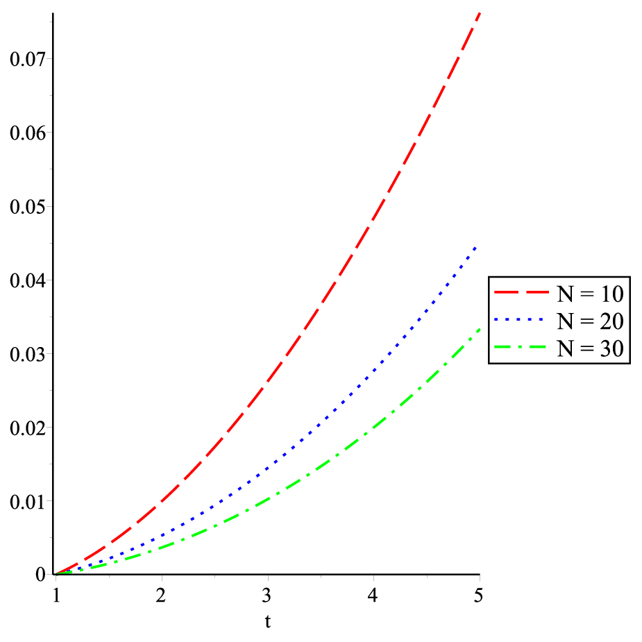
with some numerical approximations. We fix the order α⁡(t)=t/20{\alpha(t)}=t/20, and for the approximations using Theorems 3, 4 and 5, we take n=1n=1 and vary N∈{10,20,30}N\in\{10,20,30\}. The error of approximation at the point t0t_{0} is given by the absolute value of the difference between the exact and the approximation at t=t0t=t_{0}. Below we give the exact fractional derivatives of x¯\overline{x}, obtained by Lemma 1

𝔻α⁡(t)t1​x¯​(t)=1Γ⁡(2−α⁡(t))​(ln⁡t)1−α⁡(t)Dα⁡(t)t1​x¯​(t)=1Γ⁡(2−α⁡(t))​(ln⁡t)1−α⁡(t)−t​α′​(t)Γ⁡(3−α⁡(t))​(ln⁡t)2−α⁡(t)×[ln⁡(ln⁡t)+ψ⁡(1−α⁡(t))−ψ⁡(3−α⁡(t))],𝒟α⁡(t)t1​x¯​(t)=1Γ⁡(2−α⁡(t))​(ln⁡t)1−α⁡(t)−t​α′​(t)Γ⁡(3−α⁡(t))​(ln⁡t)2−α⁡(t)​[ln⁡(ln⁡t)−ψ⁡(3−α⁡(t))].\begin{array}[]{ll}{{}_{1}\mathbb{D}_{t}^{\alpha(t)}}\overline{x}(t)&=\displaystyle\frac{1}{\Gamma\left(2-{\alpha(t)}\right)}(\ln t)^{1-{\alpha(t)}}\\ {{}_{1}D_{t}^{\alpha(t)}}\overline{x}(t)&=\displaystyle\frac{1}{\Gamma\left(2-{\alpha(t)}\right)}(\ln t)^{1-{\alpha(t)}}-\frac{t{\alpha^{\prime}(t)}}{\Gamma\left(3-{\alpha(t)}\right)}(\ln t)^{2-{\alpha(t)}}\\ &\quad\displaystyle\times\left[\ln(\ln t)+\psi\left(1-{\alpha(t)}\right)-\psi\left(3-{\alpha(t)}\right)\right],\\ {{}_{1}\mathcal{D}_{t}^{\alpha(t)}}\overline{x}(t)&=\displaystyle\frac{1}{\Gamma\left(2-{\alpha(t)}\right)}(\ln t)^{1-{\alpha(t)}}-\frac{t{\alpha^{\prime}(t)}}{\Gamma\left(3-{\alpha(t)}\right)}(\ln t)^{2-{\alpha(t)}}\left[\ln(\ln t)-\psi\left(3-{\alpha(t)}\right)\right].\\ \end{array}
Refer to caption
(a) 𝔻α⁡(t)t1​x¯​(t){{}_{1}\mathbb{D}_{t}^{\alpha(t)}}\overline{x}(t)
Refer to caption
(b) Error
Figure 1: Analytic versus numerical approximations by Theorem 3.
Refer to caption
(a) Dα⁡(t)t1​x¯​(t){{}_{1}D_{t}^{\alpha(t)}}\overline{x}(t)
Refer to caption
(b) Error
Figure 2: Analytic versus numerical approximations by Theorem 4.
Refer to caption
(a) 𝒟α⁡(t)t1​x¯​(t){{}_{1}\mathcal{D}_{t}^{\alpha(t)}}\overline{x}(t)
Refer to caption
(b) Error
Figure 3: Analytic versus numerical approximations by Theorem 5.

For the right Caputo–Hadamard fractional derivatives, we take

y¯​(t)=ln⁡5t,fort∈[1,5],\overline{y}(t)=\ln\frac{5}{t},\quad\mbox{for}\quad t\in[1,5],

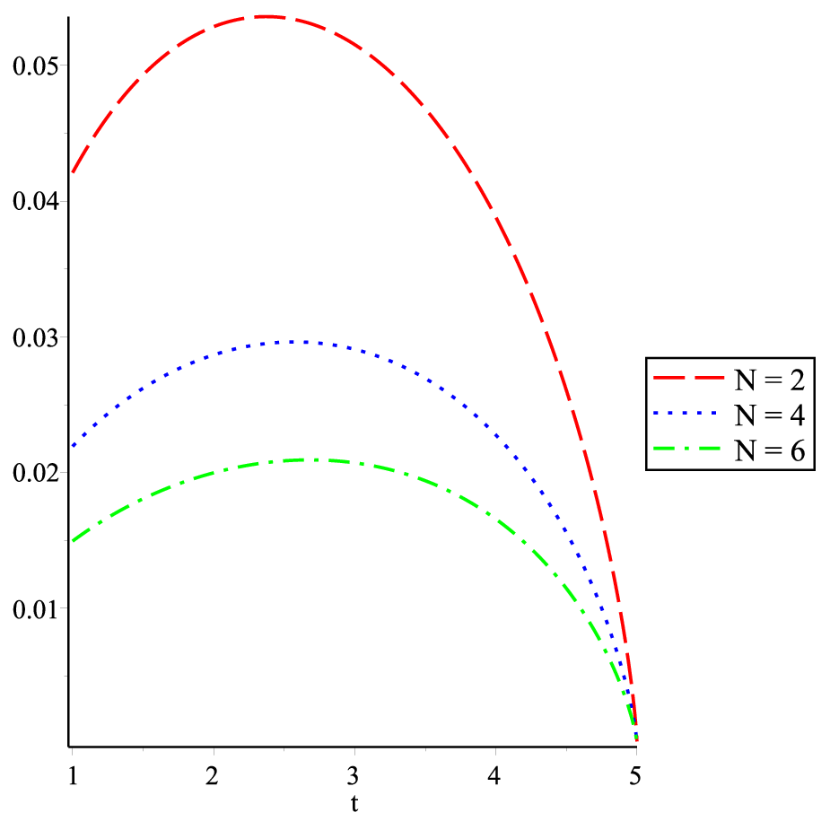
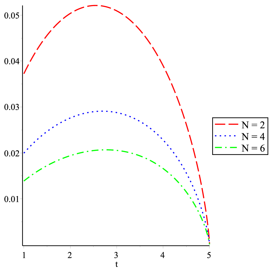
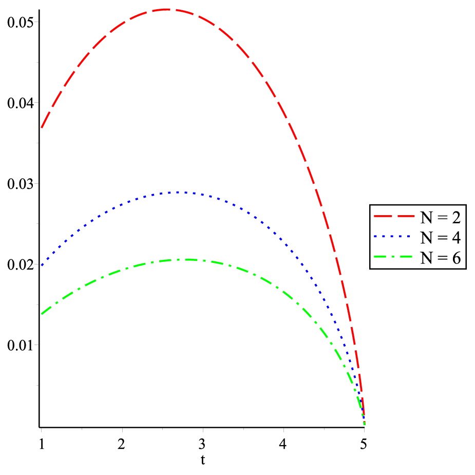
n=1n=1 and N∈{2,4,6}N\in\{2,4,6\}. The fractional derivatives are in this case given by the expressions

𝔻α⁡(t)5t​y¯​(t)=1Γ⁡(2−α⁡(t))​(ln⁡5t)1−α⁡(t)Dα⁡(t)5t​y¯​(t)=1Γ⁡(2−α⁡(t))​(ln⁡5t)1−α⁡(t)+t​α′​(t)Γ⁡(3−α⁡(t))​(ln⁡5t)2−α⁡(t)×[ln⁡(ln⁡5t)+ψ⁡(1−α⁡(t))−ψ⁡(3−α⁡(t))],𝒟α⁡(t)5t​y¯​(t)=1Γ⁡(2−α⁡(t))​(ln⁡5t)1−α⁡(t)+t​α′​(t)Γ⁡(3−α⁡(t))​(ln⁡5t)2−α⁡(t)​[ln⁡(ln⁡5t)−ψ⁡(3−α⁡(t))].\begin{array}[]{ll}{{}_{t}\mathbb{D}_{5}^{\alpha(t)}}\overline{y}(t)&=\displaystyle\frac{1}{\Gamma\left(2-{\alpha(t)}\right)}\left(\ln\frac{5}{t}\right)^{1-{\alpha(t)}}\\ {{}_{t}D_{5}^{\alpha(t)}}\overline{y}(t)&=\displaystyle\frac{1}{\Gamma\left(2-{\alpha(t)}\right)}\left(\ln\frac{5}{t}\right)^{1-{\alpha(t)}}+\frac{t{\alpha^{\prime}(t)}}{\Gamma\left(3-{\alpha(t)}\right)}\left(\ln\frac{5}{t}\right)^{2-{\alpha(t)}}\\ &\quad\displaystyle\times\left[\ln\left(\ln\frac{5}{t}\right)+\psi\left(1-{\alpha(t)}\right)-\psi\left(3-{\alpha(t)}\right)\right],\\ {{}_{t}\mathcal{D}_{5}^{\alpha(t)}}\overline{y}(t)&=\displaystyle\frac{1}{\Gamma\left(2-{\alpha(t)}\right)}\left(\ln\frac{5}{t}\right)^{1-{\alpha(t)}}+\frac{t{\alpha^{\prime}(t)}}{\Gamma\left(3-{\alpha(t)}\right)}\left(\ln\frac{5}{t}\right)^{2-{\alpha(t)}}\left[\ln\left(\ln\frac{5}{t}\right)-\psi\left(3-{\alpha(t)}\right)\right].\\ \end{array}

The results are shown in Figure 4 below.

Refer to caption
(a) 𝔻α⁡(t)5t​y¯​(t){{}_{t}\mathbb{D}_{5}^{\alpha(t)}}\overline{y}(t)
Refer to caption
(b) Error
Refer to caption
(c) Dα⁡(t)5t​y¯​(t){{}_{t}D_{5}^{\alpha(t)}}\overline{y}(t)
Refer to caption
(d) Error
Refer to caption
(e) 𝒟α⁡(t)5t​y¯​(t){{}_{t}\mathcal{D}_{5}^{\alpha(t)}}\overline{y}(t)
Refer to caption
(f) Error
Figure 4: Analytic versus numerical approximations for the right Caputo–Hadamard fractional derivatives.

Acknowledgments

This work was supported by Portuguese funds through the CIDMA - Center for Research and Development in Mathematics and Applications, and the Portuguese Foundation for Science and Technology (“FCT–-Fundação para a Ciência e a Tecnologia”), within project UID/MAT/04106/2013.

References

  • [1] T. M. Atanackovic, M. Janev, S. Pilipovic and D. Zorica, An expansion formula for fractional derivatives of variable order, Cent. Eur. J. Phys. 11 (2013), no. 10, 1350–1360.
  • [2] P.L. Butzer, A.A. Kilbas and J.J. Trujillo, Stirling functions of the second kind in the setting of difference and fractional calculus, Numer. Funct. Anal. Optim. 24 (2003), no. 7-8, 673-–711.
  • [3] C. F. M. Coimbra, Mechanics with variable-order differential operators, Ann. Phys. (8) 12 (2003), no. 11-12, 692–703.
  • [4] C. F. M. Coimbra, C. M. Soon and M. H. Kobayashi, The variable viscoelasticity operator, Annalen der Physik 14 (2005), 378–389.
  • [5] M. M. Dzherbashyan and A. B. Nersesian, Fractional derivatives and the Cauchy problem for differential equations of fractional order. Izv. Akad. Nauk Arm. SSR, Mat. 3 (1968), 3–-29.
  • [6] Y. Y Gambo, F. Jarad, D. Baleanu and T. Abdeljawad, On Caputo modification of the Hadamard fractional derivatives, Adv. Difference Equ. (2014), 2014:10 doi:10.1186/1687–1847–2014–10.
  • [7] F. Jarad, T. Abdeljawad and D. Baleanu, Caputo-type modification of the Hadamard fractional derivatives, Adv. Difference Equ. (2012), 2012:142 doi:10.1186/1687–1847–2012–142.
  • [8] Y. Lin and C. Xu, Finite difference/spectral approximations for the time-fractional diffusion equation, J. Comput. Phys. 225 (2007), no. 2, 1533–-1552.
  • [9] J. A. T. Machado, M. F. Silva, R. S. Barbosa, I. S. Jesus, C. M. Reis, M. G. Marcos and A. F. Galhano, Some applications of fractional calculus in engineering, Math. Probl. Eng. 2010 (2010), Art. ID 639801, 34 pp.
  • [10] K. S. Miller and B. Ross, An introduction to the fractional calculus and fractional differential equations, A Wiley-Interscience Publication, Wiley, New York, 1993.
  • [11] T. Odzijewicz, A. B. Malinowska and D. F. M. Torres, Noether’s theorem for fractional variational problems of variable order, Cent. Eur. J. Phys. 11 (2013), no. 6, 691–701.
  • [12] S. Pooseh, R. Almeida and D. F. M. Torres, Expansion formulas in terms of integer-order derivatives for the Hadamard fractional integral and derivative, Numer. Funct. Anal. Optim. 33 (2012), no. 3, 301–319.
  • [13] S. Pooseh, R. Almeida and D. F. M. Torres, Numerical approximations of fractional derivatives with applications, Asian J. of Control 15 (2013), no. 3, 698–712.
  • [14] L. E. S. Ramirez and C. F. M. Coimbra, On the variable order dynamics of the nonlinear wake caused by a sedimenting particle, Phys. D 240 (2011), no. 13, 1111–1118.
  • [15] S. G. Samko, A. A. Kilbas and O. I. Marichev, Fractional integrals and derivatives, Translated from the 1987 Russian original, Gordon and Breach, Yverdon, 1993.
  • [16] S. G. Samko and B. Ross, Integration and differentiation to a variable fractional order, Integral Transform. Spec. Funct. 1 (1993), no. 4, 277–300.
  • [17] H.G. Sun, W. Chen and Y.Q. Chen, Variable order fractional differential operators in anomalous diffusion modeling, Physica A. 388 (2009) 4586-–4592