Flexible Pilot Contamination Mitigation with Doppler PSD Alignment

By deploying a large number of antennas at the base station (BS), massive multiple-input multiple-output (MIMO) will be able to bring significant spectral efficiency gains. It has been regarded as one of the key enabling technologies for the next generation wireless communications [1, 4, 2, 3]. To ensure best channel estimation quality, it is desirable to allocate orthogonal uplink (UL) pilot sequences to different users so that the pilot transmissions do not interfere with each other. But within a limited time period and a limited bandwidth, there are only a limited number of orthogonal pilot sequences. As the number of users becomes large, non-orthogonal pilot sequences need to be re-used by the users served by different BSs, which leads to the so-called pilot contamination [1, 3]. Pilot contamination is one severe limiting factor in multi-cell massive MIMO systems.

Various approaches have been proposed to alleviate the pilot contamination issue in massive MIMO. Recent works include [5, 6, 12, 7, 8, 9, 11, 10, 14, 13, 15]. By staggering the UL transmission timeline of different cells, the time-shifted pilots were proposed in [5] to mitigate the pilot contamination and were further analyzed in [6]. In [7, 8, 9, 10], pilot decontamination was achieved by utilizing the fact that users with non-overlapping angles of arrival (AoA) enjoy asymptotic orthogonal covariance matrices. Phase shift pilots were exploited for channel acquisition in massive MIMO systems employing orthogonal frequency division multiplexing (OFDM) [11] and to mitigate the pilot contamination by aligning the channel power distributions in the delay-angle domain [12]. Blind methods were proposed in [13, 14] and the pilot contamination effect was shown to diminish as the data length grew. In [15], to multiplex more orthogonal pilots without losing the dimensionality for data transmission, superimposed pilots [16] were proposed for massive MIMO where pilots were sent together with data. However, constant channels were assumed in [15] to ensure enough processing gain during channel estimation to combat the data interference. In fact, constant channel gains over time are typically assumed in conventional pilot (de)contamination studies [3, 17, 1].

In this paper, we explore a new avenue to enable orthogonality among users’ UL pilots even when the users’ channels are time-varying. We demonstrate that orthogonal multiplexing of pilots in the case of Doppler fading can be achieved by aligning the Doppler power spectrum densities (PSD) of different users judiciously. Furthermore, the proposed PSD alignment enables flexible mitigation of time-varying inter-cell pilot contamination. Meanwhile, we are also able to characterize the channel estimation mean square error (MSE) performance analytically with the Doppler PSDs.

Notations: ${\sf Diag}\{\cdots\}$ denotes the diagonal matrix with diagonal elements defined inside the curly brackets. ${A}(i,j)$ refers to the $(i,j)$th entry of matrix $\bm{A}$ and $a(i)$ stands for the $i$-th entry of the vector ${\bm{a}}$. $\bm{I}$ denotes the identity matrix. ${\sf E}[\cdot]$, ${\tt Tr}(\cdot)$, $(\cdot)^{\dagger}$, $(\cdot)^{T}$, and $(\cdot)^{*}$ represent expectation, matrix trace, Hermitian operation, transpose, and conjugate operation respectively.

In a typical massive MIMO system, each BS is equipped with $M$ antennas and $K$ single-antenna users¹¹ 1 These $K$ users include all the users served by all the BSs. send UL pilots simultaneously. Assuming a narrow-band channel, e.g. a particular subcarrier in the case of OFDM transmission, we can have the following system model in the UL over $P$ successive pilot slots at one particular BS:

where ${\bm{y}}_{m}\in{\mathbb{C}}^{P}$ stands for the received signal vector at the $m$th antenna of the BS over $P$ pilot slots, $\rho_{k}$ denotes the transmitted power from user-$k$, ${\bm{X}}_{k}={\sf Diag}\{x_{k}(0),...,x_{k}(P-1)\}$ contains the transmitted pilots within the successive $P$ pilot slots from the $k$th user, ${\bm{h}}_{k,m}=[h_{k,m}(0),...,h_{k,m}(P-1)]^{T}$ represents the channel vector from user-$k$ to the $m$th antenna at the BS over the $P$ time slots, and ${\bm{w}}_{m}\in{\mathbb{C}}^{P}$ stands for the additive receiver noise. Here, we make the following assumptions:

• •

  AS1: The channel samples: $\{h_{k,m}(n)\}$ form a unit-power Gaussian stationary process with the autocorrelation function defined as²² 2 Since PSD is the Fourier transform of $r_{k}(v)$, we are assuming the same PSD for different receive antennas.: $r_{k}(v):={\sf E}[h_{k,m}(l)h_{k,m}(l+v)^{*}]$. Let ${\bm{R}}_{k}:={\sf E}[{\bm{h}}_{k,m}{\bm{h}}_{k,m}^{{\dagger}}]$ denote the covariance of the channel vector ${\bm{h}}_{k,m}$. We have $R_{k}(l,l^{\prime})=r_{k}(l^{\prime}-l)$. Meanwhile, the channels from different users are assumed independent to each other, i.e. ${\sf E}[{\bm{h}}_{k,m}{\bm{h}}_{g,m}^{{\dagger}}]={\bm{R}}_{k}\delta(k-g)$;

• •

  AS2: The receiver noise ${\bm{w}}_{m}$ is zero mean and circularly symmetric Gaussian with covariance matrix: ${\sf E}[{\bm{w}}_{m}{\bm{w}}_{m}^{{\dagger}}]=\sigma^{2}{\bm{I}}_{P}$;

• •

  AS3: The pilot sequence ${\bm{X}}_{k}$ enjoys constant unit modulus, i.e. ${\bm{X}}_{k}{\bm{X}}_{k}^{{\dagger}}={\bm{I}}$.

According to (1), we can readily obtain the MMSE estimate of user-$k$’s channel as follows:

The covariance of the channel estimation error: ${\bm{\epsilon}}:={\bm{h}}_{k,m}-{\hat{\bm{h}}}_{k,m}$ can be expressed as follows:

where

contains the interference from other users’ pilots. In the absence of those interference terms, the corresponding channel estimation MSE is

In order to obtain the interference-free MSE performance as shown in (4), we can establish the following proposition:
Proposition 1:Under AS1$\sim$3, the interference-free channel estimation performance in (4) is achieved when the pilot sequences of unit modulus satisfy the following orthogonality conditions:

where ${\bm{P}}_{k,g}={\bm{X}}_{k}^{\dagger}{\bm{X}}_{g}$.

Conventional orthogonal designs of the pilot sequences assume that the channel remains constant over the $P$ time slots containing UL pilots, where we have ${\bm{R}}_{k}={\bm{1}}\cdot{\bm{1}}^{{\dagger}}$ and ${\bm{1}}:=[1,...,1]^{T}$. Thus, the orthogonality condition in (5) naturally becomes: $\forall g\neq k$,

It can be easily seen that the above result simply informs us that the pilot sequences should be designed such that the inner product between each pair is zero. Although enjoying simplicity, the underlying assumption of a constant channel across the $P$ time slots severely limits the multiplexing capability of the conventional orthogonal designs in the case of Doppler, when the channel can be regarded constant only within a small portion of the channel coherence time [18]. In the following sections, we will address the orthogonal designs in the presence of Doppler shifts.

As $P$ gets large, we can approximate ${\bm{R}}_{k}$ by a circulant matrix ${\bm{C}}_{k}$, whose first column is defined as follows [19, 20]:

The eigenvalue decomposition (EVD) of ${\bm{C}}_{k}$ can be expressed as ${\bm{C}}_{k}={\bm{F}}^{{\dagger}}{\bm{\Lambda}}_{k}{\bm{F}}$, where ${\bm{F}}$ is the unitary $P$-point FFT matrix and ${\bm{\Lambda}}_{k}$ contains the eigenvalues. To achieve orthogonality between the UL pilots from different users in the presence of Doppler shifts, the unit modulus pilot sequences need to satisfy the condition specified in (5). By approximating ${\bm{R}}_{k}$ with ${\bm{C}}_{k}$, we can rewrite the condition in (5) as

where ${\bm{\Theta}}_{k,g}:={\bm{F}}{\bm{P}}_{k,g}{\bm{F}}^{{\dagger}}$. According to (8), the following requirement on the pilot sequences can be established:
Proposition 2:Under AS1$\sim$3, as the length of the channel observations: $P$ becomes large, the UL pilots between user-$k$ and user-$g$ at each receive antenna at the BS become orthogonal when the following condition is met:

Motivated by the structure of ${\bm{\Theta}}_{k,g}={\bm{F}}{\bm{P}}_{k,g}{\bm{F}}^{{\dagger}}$ in (9), we consider the following FFT pilot sequences:

where $\tau_{k}$ is the amount of cyclic time shifts and ${\bm{S}}_{0}$ is the base unshifted sequence with constant modulus. Note the above designs have been exploited in the LTE UL [21]. Then the matrix ${\bm{\Theta}}_{k,g}$ becomes unitary and circulant with the first column vector taking the following form:

where $\Delta\tau:=\tau_{g}-\tau_{k}$ refers to the amount of relative cyclic shifts between the user-$g$ and user-$k$. Accordingly, the diagonal matrix $\tilde{{\bm{\Lambda}}}_{g}:={\bm{\Theta}}_{k,g}{\bm{\Lambda}}_{g}{\bm{\Theta}}_{k,g}^{{\dagger}}$ is obtained by cyclicly shifting the diagonals³³ 3 Positive value means cyclic shifts towards the bottom right. of ${\bm{\Lambda}}_{g}$ by an amount of $\Delta\tau=\tau_{g}-\tau_{k}$. From Proposition 2, we can further have the following corollary:
Corollary 2.1: Under AS1$\sim$3, as the length of the channel observations: $P$ goes large, with the FFT pilot sequences in (10), the received UL pilots from user-$k$ and user-$g$ at the BS become orthogonal when the following condition is met:

where ${\mathbb{S}}_{\tau}\{\cdot\}$ stands for the operation of shifting the diagonal elements of the argument cyclicly by the amount of $\tau$.

The PSD of the sampled channel process $\{h_{k,m}(n)\}$ can be obtained by computing the discrete-time Fourier transform (DTFT) of the autocorrelation sequence $r_{k}(v)$, i.e. $S_{k}(\xi)=\sum_{v=-\infty}^{\infty}r_{k}(v)e^{-j2\pi\xi v}$. As $P$ becomes large, the $P$ eigenvalues of ${\bm{C}}_{k}$ can be approximated as the uniformly spaced samples of $S_{k}(\xi)$: $\{S_{k}([p/P]_{(-1/2,1/2]}):p=0,1,...,P-1\}$, where $[\cdot]_{(-1/2,1/2]}$ refers to the modulo operation such that the result lies in the interval $(-1/2,1/2]$. Let $f_{D,k}$ denote the maximum Doppler frequency of user-$k$. When the channel process $\{h_{k,m}(n)\}$ is obtained by sampling the underlying continuous-time fading channel at a sampling frequency of $f_{s}$, we know $S_{k}(\xi)$ is band-limited within $[-F_{k},F_{k}]$ with $F_{k}:=f_{D,k}/f_{s}$ representing the maximum discrete frequency of the PSD $S_{k}(\xi)$. In a nutshell, Corollary 2.1 informs us that, in order to ensure orthogonal pilots between two users, the amount of the relative cyclic shifts between the two users should be judiciously chosen such that the supports of their shifted PSDs are non-overlapping (see also Fig. 1). When all the users share the same maximum discrete Doppler shift $F$, we can see up to $\frac{1}{2F}$ users can transmit orthogonal pilots simultaneously and the relative cyclic shift values among users are $\left\{k\cdot 2FP,k=0,1,...,\frac{1}{2F}-1\right\}$ correspondingly.

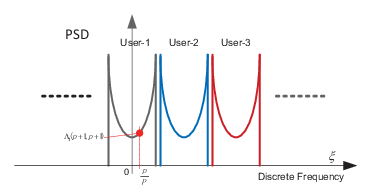
In addition to being able to support multiple orthogonal pilots in time-selective channels, the cyclic shifts in (10) can also be flexibly chosen to dodge the pilot contamination from other cells. For example, when we know there exists strong interference over the frequency supports of user-$1$ and user-$2$ in Fig. 1, we will choose the cyclic shifts such that the shifted PSDs of the desired users are non-overlapping with the interference. In Section V, we will simulate this situation and verify the effectiveness of our designs.

In the case of multiple users, we can get the following result characterizing the channel estimation MSE performance (see detailed proof in Appendix A):
Proposition 3: When the pilot sequences are designed as in (10), as $P$ goes large, under AS1$\sim$3, the MSE of each element of ${\bm{h}}_{k,m}$ can be approximated as follows:

where $S_{k}(\xi)$ denotes the PSD of user-$k$, and $\tilde{S}_{g}(\xi):=S_{g}(\xi-(\tau_{g}-\tau_{k})/{P})$.

Assuming the Jakes’s fading model [24] (a.k.a. Clarke’s model), the autocorrelation function: $r_{k}(v)$ can be expressed as $r_{k}(v)=J_{0}(2\pi F_{k}v)$, where $f_{D,k}$ denotes the maximum Doppler frequency of user-$k$, $f_{s}$ represents the channel sampling frequency, $F_{k}:=f_{D,k}/f_{s}$ is the normalized Doppler frequency, and $J_{0}(\cdot)$ is the zeroth-order Bessel function of the first kind. When $F_{k}\leq\frac{1}{2}$, the PSD of the discrete channel process: $\{h_{k,m}(n)\}$ can be expressed as follows:

By combining (14) and (13), as the orthogonality conditions in (5) or (12) are satisfied, the channel estimation MSE in (13) can be approximated as follows:

where $\alpha:=\pi F_{k}\sigma^{2}/\rho_{k}$.

Let’s now consider the LTE numerology [21]. For a carrier frequency of $2$GHz, as the user’s moving speed is around $30$km/h, we see the max Doppler shift is about $f_{D}=55$Hz. Considering each OFDM symbol lasts $T_{s}=66.67\mu$s, the channel sampling frequency can be chosen as $f_{s}=1/(3T_{s})=5$kHz for OFDM. The maximum normalized Doppler shift is then $F_{k}=f_{D}/f_{s}=0.011\ll 1$. Thus, when the receiving signal-to-noise ratio (SNR) of the pilots is not too small, e.g. $>-10$dB, we only need to consider the first case in (15). The following corollary can be established from Proposition 3 (see Appendix B for detailed proof):
Corollary 3.1: In a communication system with $\pi F_{k}\ll\rho_{k}/\sigma^{2}$, under the classical Clarke’s fading, as the orthogonality conditions in (5) are satisfied and the length of the channel observations: $P$ goes large, under the assumptions AS1$\sim$3, the MSE of each element of ${\bm{h}}_{k,m}$ can be approximated as follows:

and the following processing gain⁴⁴ 4 The processing gain here refers to the amount of SNR improvement during the channel estimation relative to the observation SNR [18]. in dB scale can be achieved:

To verify our orthogonal designs for Doppler, we simulate a TDD reciprocal massive MIMO system as configured in Fig. 2, where $8$ users experience the Jakes’s flat-fading channels with the same Doppler frequency $f_{D}=10$Hz and the channel gains towards the serving BS. Inter-cell pilot contamination is modelled as a stationary random process with uniform PSD in the discrete frequency range: $[-3/8,+3/8]$. The following system parameters are assumed during the simulations:

• •

  OFDM symbol duration⁵⁵ 5 Since all the simulations here are on a particular subcarrier, the exact number of subcarriers within one OFDM symbol does not really matter. : $T_{s}=66.67\mu$s; channel sampling frequency: $f_{s}=\frac{1}{3T_{s}}=5$kHz;

• •

  Antenna array size at the BS: $M=128$; different antennas at the BS are assumed independent.

Fig. 3 compares the channel estimation MSE normalized by the average channel power (nMSE) with different pilot sequences designs. Fig. 4 depicts the achieved processing gains of our scheme and the conventional ones. Clearly, our proposed pilot designs exhibit significant improvement in both MSE and processing gain with respect to the convention pilots. In Fig. 5, we plot the sum downlink (DL) spectral efficiency when the BS performs the matched-filter beamforming [1] to the served users. Exploiting the TDD reciprocity, the DL channel states are obtained from the estimated UL channels with the previous UL pilots as illustrated in Fig. 2. We see more accurate DL channel state information (CSI) at the BS enabled by aligning the PSDs appropriately translates to higher DL spectral efficiency in the presence of time-varying pilot contamination.

In this paper, we have developed a novel pilot design principle in the case of Doppler fading. Through flexibly aligning the PSDs, pilot decontamination can be achieved and more users’ channels can be sounded simultaneously even with high Doppler. Meanwhile, we have derived analytical formulae characterizing the channel estimation MSE performance with our proposed pilot designs. Numerical simulations corroborate our designs and demonstrate that our proposed designs outperform the conventional designs significantly as the length of the channel observations $P$ goes large. In practice, to obtain the autocorrelation matrix at the BS involves an overhead proportional to $P^{2}$, which would limit the maximum length of the channel observations.

The proposed PSD aligning can serve as a new complementary design philosophy for the UL pilots to address the notorious pilot contamination in massive MIMO. In particular, our proposed PSD aligning can be naturally combined with those decontamination schemes exploiting the spatial separability to handle the cases with overlapping AoAs.

When $P$ goes to infinity, by approximating ${\bm{R}}_{k}$ (${\bm{R}}_{g}$) with a circulant matrix ${\bm{C}}_{k}$ (${\bm{C}}_{g}$), we can rewrite (3) as

Following the results in [19], the MSE of each element of ${\bm{h}}_{k,m}$ can then be approximated as:

where $\lambda_{k,p}$ is the $p$-th eigenvalue of ${\bm{\Lambda}}_{k}$, $S_{k}(\xi)$ denotes the PSD of user-$k$, and $\tilde{S}_{g}(\xi):=S_{g}(\xi-(\tau_{g}-\tau_{k})/{P})$.

In a communication system with $\pi F_{k}\ll\rho_{k}/\sigma^{2}$, we can focus on the case with $\alpha\ll 1$ in (15). Carrying out the Taylor series expansion in the case with $\alpha\ll 1$, we can obtain

Since $\alpha\ll 1$, the first-order term in (20) already provides a close approximate. Thus we have the desired result as follows:

References

- [1] T. L. Marzetta, “Noncooperative cellular wireless with unlimited numbers of base station antennas,” IEEE Trans. Wireless Commun., vol. 9, no. 11, pp. 3590-3600, Nov. 2010.
- [2] E. G. Larsson, O. Edfors, F. Tufvesson, and T. L. Marzetta, “Massive MIMO for next generation wireless systems,” IEEE Commun. Mag., vol. 52, no. 2, pp. 186-195, Feb. 2014.
- [3] L. Lu, G. Y. Li, A. L. Swindlehurst, A. Ashikhmin, and R. Zhang, “An overview of Massive MIMO: Benefits and challenges,” IEEE J. Sel. Topics Signal Process., vol. 8, no. 5, pp. 742-758, Oct. 2014.
- [4] F. Rusek, D. Persson, B. K. Lau, E. G. Larsson, T. L. Marzetta, O. Edfors, and F. Tufvesson, “Scaling up MIMO: Opportunities and challenges with very large arrays ,” IEEE Signal Process. Mag., vol. 30, no. 1, pp. 40-60, Jan. 2013.
- [5] F. Fernandes, A. Ashikhmin, and T. L. Marzetta, “Inter-cell interference in noncooperative TDD large scale antenna systems,” IEEE J. Sel. Areas Commun., vol. 31, no. 2, pp. 192-201, Feb. 2013.
- [6] S. Jin, X. Wang, Z. Li, K.-K. Wong, Y. Huang, and X. Tang, “On massive MIMO zero-forcing transceiver using time-shifted pilots” IEEE Trans. Veh. Technol., vol. 65, no. 1, pp. 59-74, Jan. 2016.
- [7] H. Yin, D. Gesbert, M. Filippou, and Y. Liu, “A coordinated approach to channel estimation in large-scale multiple-antenna systems,” IEEE. J. Sel. Areas. Commun., vol. 31, no. 2, pp. 264-273, Feb. 2013.
- [8] H. Yin, D. Gesbert, and L. Cottatellucci, “Dealing with interference in distributed large-scale MIMO systems: A statistical approach,” IEEE J. Sel. Topics Signal Process., vol. 8, no. 5, pp. 942-953, Oct. 2014.
- [9] L. You, X. Gao, X.-G. Xia, N. Ma, and Y. Peng, “Pilot reuse for massive MIMO transmission over spatially correlated Rayleigh fading channels,” IEEE Trans. Wireless Commun., vol. 14, no. 6, pp. 3352-3366, Jun. 2015.
- [10] H. Yin, L. Cottatellucci, D. Gesbert, R. R. Muller, and G. He, “Robust pilot decontamination based on joint angle and power domain discrimination,” IEEE Trans. Signal Process., vol. 64, no. 11, pp. 2990-3003, Jun. 2016.
- [11] L. You, X. Gao, A. L. Swindlehurst, and W. Zhong, “Channel acquisition for massive MIMO-OFDM with adjustable phase shift pilots,” IEEE Trans. Signal Process., vol. 64, no. 6, pp. 1461-1476, Mar. 2016.
- [12] X. Luo, X. Zhang, H. Qian, and K. Kang, “Pilot Decontamination via PDP alignment,” to appear in Proc. IEEE GLOBECOM, Washington D.C., USA, Dec. 2016. Also available at: arXiv:1607.07537 [cs.IT].
- [13] R. R. Muller, L, Cottatellucci, and M. Vehkapera, “Blind pilot decontamination,” IEEE J. Sel. Topics Signal Process., vol. 8, no. 5, pp. 773-786, Oct. 2014.
- [14] D. Hu, L. He, and X. Wang, “Semi-blind pilot decontamination for massive MIMO systems,” IEEE Trans. Wireless Commun., vol. 15, no. 1, pp. 525-536, Jan. 2016.
- [15] K. Upadhya, S. A. Vorobyov, and M. Vehkapera, “Superimposed pilots: An alternative pilot structure to mitigate pilot contamination in massive MIMO,” in Proc. ICASSP, pp. 3366-3370, Shanghai, China, Mar. 2016.
- [16] S. He, J. K. Tugnait, and X. Meng, “On superimposed training for MIMO channel estimation and symbol detection,” IEEE Trans. Signal Process., vol. 55, no. 6, pp. 3007-3021, Jun. 2007.
- [17] J. Jose, A. Ashikhmin, T. L. Marzetta, and S. Vishwanath, “Pilot contamination and precoding in multi-cell TDD systems,” IEEE Trans. Wireless Commun., vol. 10, no. 8, pp. 2640-2651, Aug. 2011.
- [18] J. G. Proakis and M. Salehi, Digital Communications. New York, USA: McGraw-Hill, 2008.
- [19] A. Adhikary, J. Nam, J. Y. Ahn, and G. Caire, “Joint spatial division and multiplexing-The large-scale array regime,” IEEE. Trans. Inf. Theory, vol. 59, no. 10, pp. 6441-6463, Oct. 2013.
- [20] R. Gray, Toeplitz and Circulant Matrices: A Review. The Netherlands: Now Publishers, 2006.
- [21] S. Sesia, I. Toufik, and M. Baker, LTE - The UMTS Long Term Evolution: From Theory to Practice. West Sussex, U.K.: John Wiley Sons Ltd., 2nd Ed., 2011.
- [22] Y. Li, L. J. Cimini, and N. R. Sollenberger, “Robust channel estimation for OFDM systems with rapid dispersive fading channels,” IEEE Trans. Commun., vol. 46, no. 7, pp. 902-915, Jul. 1998.
- [23] X. Luo and X. Zhang, “Flexible pilot contamination mitigation with Doppler PSD alignment,” arXiv:1607.07548 [cs.IT], Jul. 2016.
- [24] W. C. Jakes, Microwave Mobile Communictions. West Sussex, U.K.: John Wiley Sons Ltd., 1975.