Pilot Decontamination via PDP Alignment

Massive multiple-input multiple-output (MIMO) has been regarded as one of the enabling technologies in next generation wireless communications[1, 4, 2, 3]. Considering the large number of antennas at the base station (BS), it becomes almost imperative to rely on the time-division duplexing (TDD) channel reciprocity to learn the downlink (DL) channel state information (CSI) from the uplink (UL) channel measurements at the BS to avoid the huge overhead for CSI feedback as in frequency-division duplexing (FDD) systems. Even though the antenna array size is large at the BS, each user is only equipped with a few antennas, e.g. only one antenna. A user just needs to send one UL pilot sequence per transmit antenna to facilitate the BSs to acquire reliable estimates of the corresponding many UL channels from the user to the large antenna array at the BS.

To ensure best CSI estimation quality, we want to allocate orthogonal UL pilot sequences to different users so that the pilot transmissions do not interfere with each other. But in reality, within a limited time period and a limited bandwidth, there are only a limited number of orthogonal pilot sequences. As the number of users becomes large, non-orthogonal pilot sequences are re-used by the users served by different BSs, which gives rise to the so-called pilot contamination [1, 3] and is one limiting factor in multi-cell massive MIMO systems.

Various approaches have been proposed to alleviate the pilot contamination issue in massive MIMO. Recent works include [5, 6, 7, 9, 8]. See also [3] and references therein for a brief overview. In [5] and [6], pilot decontamination was achieved by utilizing the fact that users with non-overlapping angles of arrival (AoA) enjoy asymptotic orthogonal covariance matrices. In [7], AoA diversity and amplitude-based projection were jointly exploited to null the pilot contamination and achieve better channel estimation. A blind singular value decomposition (SVD) based method was proposed in [8] to separate the signal subspace from the interference subspace. In [9], least-squares (LS) channel estimate was derived by treating the blindly detected UL data as pilot symbols and the pilot contamination effect was shown to diminish as the data length grew.

Unlike previous studies where a single narrow-band channel was typically assumed, in this paper, we look into the issue of intra-cell pilot orthogonalization and schemes for mitigating the inter-cell pilot contamination with a realistic massive MIMO OFDM system model. First, we examine how to align the power-delay profiles (PDP, a.k.a. delay power spectrum in [10]) of different users served by one BS so that the pilots sent within one common OFDM symbol are orthogonal. From the aligning rule, we can see much more users can be sounded in the same OFDM symbol as their channels are sparse in time. In the case of massive MIMO, to alleviate the pilot contamination when the schemes in [5, 6, 7] do not apply well due to interfering users’ overlapping AoAs, we further propose to exploit the fact that different paths in time are associated with different AoAs and the pilot contamination can be significantly reduced by aligning the PDPs of the users served by different BSs appropriately. Thus, PDP aligning can serve as the new baseline design philosophy for massive MIMO UL pilots.

This paper is organized as follows: Section II describes the massive MIMO OFDM system model and the channel model. Section III provides a sufficient condition for orthogonal pilots design through PDP aligning, which is also applicable to conventional MIMO systems. Then we explain how to mitigate the pilot interference in the case of massive MIMO by PDP alignment in Section IV. Low-complexity pilot designs are provided in Section V. Corroborating simulation results are provided in Section VI and Section VII concludes the paper.

Notations: ${\sf Diag}\{\cdots\}$ denotes the diagonal matrix with diagonal elements defined inside the curly brackets. ${A}(i,j)$ refers to the $(i,j)$th entry of matrix $\bm{A}$ and $a(i)$ stands for the $i$-th entry of the vector ${\bm{a}}$. $\bm{I}_{N}$ denotes the $N\times N$ identity matrix. ${\sf E}[\cdot]$, ${\tt Tr}(\cdot)$, $(\cdot)^{\dagger}$, $(\cdot)^{T}$, and $(\cdot)^{*}$ represent expectation, matrix trace, Hermitian operation, transpose, and conjugate operation respectively.

We consider an MIMO-OFDM system with $B$ macro BSs. Each BS is equipped with a massive antenna array of size $M$ and serves $K$ single-antenna users. Regarding the OFDM waveform, we adopt the following notations:

• •

  $N$: total number of sub-carriers, a.k.a. tones;

• •

  $T$: time duration of one OFDM symbol;

• •

  $T_{c}:=T/N$: time duration of one chip;

• •

  $N_{cp}$: cyclic prefix length in $T_{c}$.

As the delay spread of each user’s channel is less than $N_{cp}$, after standard OFDM receiver processing, the received signal at the $m$-th antenna in BS-$b$ can be expressed as

where ${\bm{y}}_{m}^{(b)}$ is an $N\times 1$ vector containing the received signal over all the tones and the summation is taken over all the BSs and all the served users. For user-$k$ in BS-$l$ (we will denote it as user-$(l,k)$ in the sequel), $\rho_{k}^{(l)}$ denotes the transmitted power over each tone and ${\bm{S}}_{k}^{(l)}$ is an $N\times N$ diagonal matrix with diagonal entries being the transmitted pilot sequence. The frequency response of the channel from user-$(l,k)$ to the $m$-th antenna at BS-$b$ is ${\bm{H}}_{k,m}^{(l,b)}$ and ${\bm{w}}_{m}^{(b)}$ represents the receiver noise with covariance ${\sf E}[{\bm{w}}_{m}^{(b)}{\bm{w}}_{m}^{(b)\dagger}]=\sigma^{2}{\bm{I}}$.

The channel frequency response is the discrete Fourier transform (DFT) of the corresponding channel impulse response (CIR) in time domain, i.e.

where ${\bm{F}}$ stands for the unitary FFT matrix defined as ${F}(k,n)=\exp\{-j2\pi(k-1)(n-1)/N\}/\sqrt{N}$ and ${\bm{h}}_{k,m}^{(l,b)}$ is the CIR with the following PDP:

where we have assumed the channels from one user to the antennas at one BS share a common PDP. Assuming uncorrelated scattering as in [10], i.e. the scattering at two different paths is uncorrelated, the PDP matrix ${\bm{P}}_{k}^{(l,b)}$ becomes diagonal. Combining (1) and (2), we have

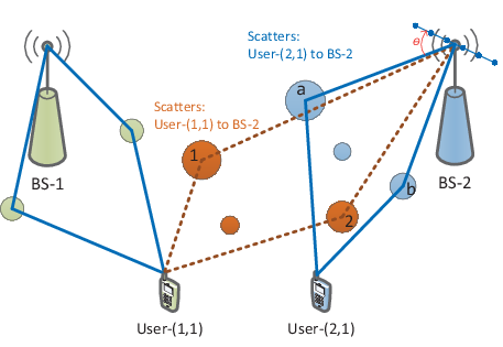
In order to characterize the spatial covariance among multiple receive antennas at the BSs, we adopt the multi-path spatial channel model (SCM) defined in [11] and [12], which is illustrated in Fig. 1. Each resolvable channel path corresponds to one independent scatterer including $Q$ sub-paths:

where the arriving angles: $\{\theta_{k,n,q}^{(l,b)}\}_{q=1}^{Q}$ of the sub-paths are uniformly distributed within the angle spread (AS) of this path, the phases: $\{\phi_{q}\}$ are drawn from a uniform distribution over $[0,2\pi]$, and the vector ${\bm{a}}(\theta)$ stands for the steering vector of the receive antenna array when the AoA of the incoming path is $\theta$. Assuming a uniform linear array (ULA), the steering vector can be expressed as:

where $D$ is the antenna spacing and $\lambda$ denotes the carrier wavelength. As $M\rightarrow\infty$, we can obtain one noticeable result as follows: $\forall\theta_{1}\neq\theta_{2}\in(0,\pi)$, as $D<\lambda/2$,

where we have assumed $\theta_{1}$ and $\theta_{2}$ are independent of $M$. This result indicates the asymptotic orthogonality of the paths arriving from different angles. In the following sections, we will take advantage of this important fact to design UL pilots.

Using the observation in (4), we can obtain the MMSE estimate for the channel between user-$(b,u)$ and the $m$-th antenna at BS-$b$ as follows:

where

contains the interference from the intra-cell users, and

includes the inter-cell interference. Note in the above derivation, we have assumed the channels among different users are independent.

Defining the channel estimation error as ${\bm{\epsilon}}:={{\bm{h}}}_{u,m}^{(b,b)}-\hat{{\bm{h}}}_{u,m}^{(b,b)}$, we can obtain its covariance as follows:

Without loss of generality, we let ${\bm{S}}_{u}^{(b)}{\bm{S}}_{u}^{(b)\dagger}={\bm{I}}$, i.e. the pilot sequence enjoys constant unit modulus. Then, we can rewrite (9) as

where $\tilde{\bm{\Delta}}_{1}={\bm{F}}^{\dagger}{\bm{S}}_{u}^{(b)\dagger}{\bm{\Delta}}_{1}{\bm{S}}_{u}^{(b)}{\bm{F}}$ and $\tilde{\bm{\Delta}}_{2}={\bm{F}}^{\dagger}{\bm{S}}_{u}^{(b)\dagger}{\bm{\Delta}}_{2}{\bm{S}}_{u}^{(b)}{\bm{F}}$. In the absence of interference, the corresponding MSE covariance can be computed accordingly as

To achieve the orthogonality between the received pilots from the interfering user-$(l,k)$ and the targeted user-$(b,u)$, from (10) and (11), we need to ensure ${\bm{S}}_{u}^{(b)}$ and ${\bm{S}}_{k}^{(l)}$ satisfy the following condition:

where ${\bm{\Theta}}:={\bm{F}}^{\dagger}{\bm{S}}_{u}^{(b)\dagger}{\bm{S}}_{k}^{(l)}{\bm{F}}$. From (12), we can establish the following requirement on the pilot sequences:
Proposition 1: To achieve orthogonality between the UL pilots from user-$(l,k)$ and user-$(b,u)$ at each receive antenna in the BS, the constant unit-modulus pilot sequences need to satisfy the following condition:

In the following discussions, we will assume the following pilot sequences as in the LTE UL [13]:

where $\tau_{l,k}$ is the amount of cyclic time shifts and ${\bm{S}}_{0}$ is the base unshifted sequence with constant modulus. With the above sequence designs, the matrix ${\bm{\Theta}}$ becomes unitary and circulant with the first column vector taking the following form:

where $\Delta\tau:=\tau_{l,k}-\tau_{b,u}$ refers to the amount of relative cyclic shifts between the two users. From (13), we obtain the corresponding requirement on $\Delta\tau$ as:

where $\tilde{\bm{P}}_{k}^{(l,b)}:={\bm{\Theta}}{\bm{P}}_{k}^{(l,b)}{\bm{\Theta}}^{\dagger}$ is the result of cyclicly shifting the diagonals of ${\bm{P}}_{k}^{(l,b)}$ by $-\Delta\tau$. The orthogonality condition in (16) simply states that, to ensure orthogonal pilots between two users, the amount of the relative cyclic shifts between the two users should be chosen such that the supports of the shifted PDPs are non-overlapping.

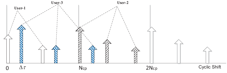
Conventional designs assume that the PDPs of all users are confined within the first $N_{cp}$ taps [13]. In order to ensure orthogonality in (16), we see up to $\frac{N}{N_{cp}}$ users¹¹ 1 Here we assume $N_{cp}$ divides $N$. Otherwise, we can do flooring: $\lfloor\frac{N}{N_{cp}}\rfloor$. can transmit pilots in the same OFDM symbol and the relative cyclic shift values among users are: $\Delta\tau=kN_{cp},k=0,1,...,N/N_{cp}-1$. In fact, from the general condition specified in (16), we can easily see that the amount of cyclic shifts required can be well below $N_{cp}$ when the PDPs are sparse in time (see also Fig. 2).

Even though we can exploit the channel sparsity and the proposed PDP alignment as illustrated in Fig. 2, it is clear that there are only a limited number of orthogonal pilot sequences available within the channel coherence time. Pilot contamination refers to the fact that, as $B\cdot K$ becomes large, we can not provide each user an orthogonal pilot sequence. Instead, a typical solution is to orthogonalize the users served by a common BS while allowing non-orthogonal pilot sequences among users served by different BSs. In the next section, we will examine a novel scheme applicable in the case of massive MIMO to reduce the inter-cell interference.

Assume the users $\{1,...,K_{l}\}$ served by BS-$l$ are assigned the cyclic shifts $\{\tau_{l,1},...,\tau_{l,K_{l}}\}$ in (14) and the orthogonality condition in (16) is met with these cyclic shifts. Since all the orthogonal cyclic shift resources are used to enable intra-cell orthogonality, the users served by different BSs have to reuse the same set of pilot sequences. From (4), we can have the following signal model at the $m$-th antenna of BS-$b$:

Then, we can obtain

where $\breve{\bm{h}}_{m}^{(l,b)}:=\sum_{k=1}^{K_{l}}\sqrt{\rho_{k}^{(l)}}{\bm{\Theta}}_{k}^{(l)}{\bm{h}}_{k,m}^{(l,b)}$ is the aggregate channel of all those $K_{l}$ non-interfering intra-cell orthogonal users served by BS-$l$, ${\bm{\Theta}}_{k}^{(l)}:={\bm{F}}^{\dagger}{\bm{S}}_{0}^{\dagger}{\bm{S}}_{k}^{(l)}{\bm{F}}$ is a circulant matrix with the first column vector defined as in (15) with $\Delta\tau=\tau_{l,k}$, and the noise term ${\bm{\omega}}_{m}^{(b)}$ has the same covariance as ${\bm{w}}_{m}^{(b)}$. Stacking the $n$-th taps of $\{{\bm{z}}_{m}^{(b)}\}_{m=1}^{M}$ into an $M\times 1$ vector as: ${\bm{g}}_{n}^{(b)}:=[{z}_{1}^{(b)}(n),...,{z}_{M}^{(b)}(n)]^{T}$, we can get

where ${\bm{h}}_{n}^{(l,b)}$ denotes the vector of the $n$-th taps in the aggregate channels from the orthogonal users served by BS-$l$ to BS-$b$, i.e. ${\bm{h}}_{n}^{(l,b)}:=[\breve{h}_{1}^{(l,b)}(n),...,\breve{h}_{M}^{(l,b)}(n)]^{T}$ and ${\bm{\omega}}^{(b)}:=[{\omega}_{1}^{(b)}(n),...,{\omega}_{M}^{(b)}(n)]^{T}$. Since the circulant matrix ${\bm{\Theta}}_{k}^{(l)}$ carries out cyclic shift operation, we have

Note that for channels of limited delay spread, only a few users will have non-zero contribution toward the aggregated channel tap in (20).

Denoting the spatial covariance matrix of the $n$-th taps in the aggregate channels from users in BS-$l$ to BS-$b$ across the $M$ BS antennas as ${\bm{C}}_{n}^{(l,b)}$, i.e. ${\bm{C}}_{n}^{(l,b)}:={\sf E}\left[{\bm{h}}_{n}^{(l,b)}{\bm{h}}_{n}^{(l,b)\dagger}\right]$, with the signal model in (19), we can derive the MMSE estimate of the desired channel ${\bm{h}}_{n}^{(b,b)}$ as:

The covariance of the estimation error vector: ${\bm{\epsilon}}_{n}^{(b,b)}:={\bm{h}}_{n}^{(b,b)}-\hat{\bm{h}}_{n}^{(b,b)}$ can be found as follows:

Let $\sum_{l=1,l\neq b}^{B}{\bm{C}}_{n}^{(l,b)}={\bm{U}}{\bm{\Sigma}}{\bm{U}}^{\dagger}$ and ${\bm{C}}_{n}^{(b,b)}={\bm{V}}{\bm{\Lambda}}{\bm{V}}^{\dagger}$, where $\bm{U}$ ($\bm{V}$) is an $M\times r$ ($M\times r^{\prime}$) matrix consisting of $r$ ($r^{\prime}$) eigenvectors and $\bm{\Sigma}$ ($\bm{\Lambda}$) is an $r\times r$ ($r^{\prime}\times r^{\prime}$) diagonal matrix consisting of $r$ ($r^{\prime}$) non-zero eigenvalues. From (22), we get

where the residual matrix ${\bm{R}}_{n}^{(b)}$ is of the following form

To obtain a reliable estimate of ${\bm{h}}_{n}^{(b,b)}$, we would like to make the subspaces spanned by the interference term and the signal term as orthogonal as possible. When ${\sf span}\{\bm{U}\}\perp{\sf span}\{\bm{V}\}$, we have ${\bm{R}}_{n}^{(b)}={\bm{0}}$ and achieve the interference-free estimation performance.

Channel taps (a.k.a. paths) of different time delays are originating from different scattering clusters. Similar to (7), when the angles of arrival (AoA) of two paths do not overlap, it has been shown that the associated covariance matrices span orthogonal subspaces asymptotically as $M\rightarrow\infty$ [5, 6, 14]. Notice that the estimation error due to non-orthogonal pilots in (24) depends on the set of cyclic shifts: $\{\tau_{l,k}\}$. Through exploiting the diversity in the covariance matrices of different paths, we can judiciously choose the set of cyclic shift values: $\{\tau_{l,k}\}$ in (14) to minimize the amount of extra estimation error due to inter-cell interference. This set of optimal cyclic shift values will align the PDPs of the users with non-orthogonal pilots in a way to mitigate the inter-cell pilot contamination. In Fig. 1, the composite AoAs of user-$(1,1)$ and user-$(2,1)$ at BS-$2$ are similar and the existing approaches in [5, 7] will not be able to separate them well. In other words, without alignment, there will be strong pilot contamination between the two users. However, after aligning path-$1$ to path-$b$ and path-$2$ to path-$a$, we can expect near interference-free performance in estimating the channels from user-$(2,1)$ to BS-$2$.

To optimize the overall system performance, we need to solve the following optimal PDP alignment problem:

where the constraint in (26) comes from the intra-cell orthogonality requirement in (16).

The PDP alignment problem in (25) requires exhaustive searches over all possible cyclic time shifts of all served users. It becomes too complex to be implemented in practice as the number of served users goes large. Low-complexity designs are worthwhile and will be discussed in Section V.

Summarizing, after aligning different users’ PDPs appropriately, we can achieve the following two benefits at the same time:

• •

  1). For sparse PDPs, more users served by a common BS can transmit orthogonal pilot sequences within one OFDM symbol;

• •

  2). When the aligned interfering paths have non-overlapping AoAs with the desired path, asymptotic inter-cell interference-free estimation performance can be achieved as the size of the massive antenna array goes large, i.e. $M\rightarrow\infty$.

The optimal solution of the optimization problem in (25) is hard to find due to the complex structure of the objective function. Instead, we can make some simplifications and try to solve easier problems. In the following discussions, we will assume that the delay spread of users’ channels is $N_{cp}$ chips.

In this section, we simulate the system as illustrated in Fig. 1, where there are two neighboring cell-edge users creating strong inter-cell interference. Other simulation parameters and assumptions are listed as follows:

1. 1.

   OFDM configurations²² 2 We follow the numerology in LTE [13].: $T=66.67\mu$s ($1/T=15$kHz), $N=128$, $N_{cp}=8$;

2. 2.

   Each BS is equipped with a ULA of size $M=50$ and antenna spacing $D=\lambda/2$. Each path toward the BS is generated according to the SCM defined in [11];

3. 3.

   Both uniform and exponential PDPs are simulated. For the uniform PDP, we have $P_{n}=P_{0},\forall n\in[1,N_{cp}]$. For the exponential PDP, we have $P_{n}=P_{0}e^{-0.6(n-1)}$, $\forall n\in[1,N_{cp}]$.

4. 4.

   User-$(1,1)$ and user-$(2,1)$ are close to each other but are served by different BSs. They share the same scatterers toward each BS, i.e. their visibility regions (VR) are overlapping [12];

5. 5.

   User-$(1,1)$ and user-$(2,1)$ are assigned to the same tone group as defined in Section V-B and the optimal PDP alignment is found by minimizing the cost function in (31).

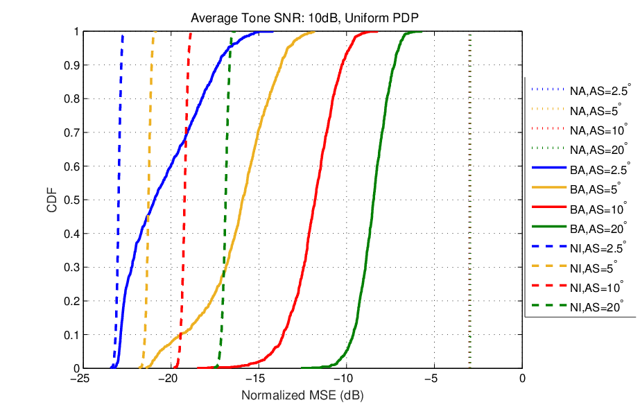
In Fig. 5, we show the cumulative distribution functions (CDF) of the normalized mean-square error (MSE)³³ 3 Normalized MSE is defined as: ${\tt NMSE}:=\frac{\sum_{l=1}^{2}\sum_{n=1}^{N_{cp}}\|\hat{\bm{h}}_{n}^{(l,l)}-{\bm{h}}_{n}^{(l,l)}\|^{2}}{\sum_{l=1}^{2}\sum_{n=1}^{N_{cp}}\|{\bm{h}}_{n}^{(l,l)}\|^{2}}$. of the estimated channels with and without PDP alignment. In each one of the $1000$ Monte-Carlo runs, the second-order statistics of the channel taps are randomly generated according to the SCM. The PDP alignment in (31) is based on the second-order statistics to mitigate the pilot contamination. From Fig. 5, we see the exponential PDP can provide better decontamination than the uniform PDP. Compared with the case without alignment, optimal PDP aligning can bring about $13$dB improvement in UL channel estimation at the median point, i.e. $50\%$ in the CDF curve.

In Fig. 6, we examine the PDP alignment performance for different AS values. From the plotted curves, we see the PDP alignment favors the scattering environment with a small AS. In Fig. 7, we compare the sum of DL spectral efficiency to the two users in Fig. 1 when the BSs formulate the DL matched-filter precoding vectors with the estimated UL channnels assuming TDD channel reciprocity. It can be observed that the achieved spectral efficiency after PDP aligning is pretty close to that without UL pilot contamination.

In this paper, relying on a realistic massive MIMO OFDM system model, we have addressed the issue of pilot contamination and proposed to rely on PDP aligning to mitigate this type of inter-cell pilot interference. On one hand, we have shown the UL pilots from the users served by one common BS can be made orthogonal through PDP aligning. On the other hand, due to the massive amount of antennas at the BS, we have shown that PDP alignment can also help to alleviate the pilot contamination thanks to the fact that different paths in time are originating from different AoAs. Numerical simulations validate that the pilot contamination can be significantly reduced through aligning the PDPs of the users served by different BSs appropriately. The proposed PDP aligning can serve as the new baseline design philosophy for the UL pilots in massive MIMO.

References

- [1] T. L. Marzetta, “Noncooperative cellular wireless with unlimited numbers of base station antennas,” IEEE Trans. Wireless Commun., vol. 9, no. 11, pp. 3590-3600, Nov. 2010.
- [2] E. G. Larsson, O. Edfors, F. Tufvesson, and T. L. Marzetta, “Massive MIMO for next generation wireless systems,” IEEE Commun. Mag., vol. 52, no. 2, pp. 186-195, Feb. 2014.
- [3] L. Lu, G. Y. Li, A. L. Swindlehurst, A. Ashikhmin, and R. Zhang, “An overview of Massive MIMO: Benefits and challenges,” IEEE J. Sel. Topics Signal Process., vol. 8, no. 5, pp. 742-758, Oct. 2014.
- [4] F. Rusek, D. Persson, B. K. Lau, E. G. Larsson, T. L. Marzetta, O. Edfors, and F. Tufvesson, “Scaling up MIMO: Opportunities and challenges with very large arrays ,” IEEE Signal Process. Mag., vol. 30, no. 1, pp. 40-60, Jan. 2013.
- [5] H. Yin, D. Gesbert, M. Filippou, and Y. Liu, “A coordinated approach to channel estimation in large-scale multiple-antenna systems,” IEEE. J. Sel. Areas. Commun., vol. 31, no. 2, pp. 264-273, Feb. 2013.
- [6] H. Yin, D. Gesbert, and L. Cottatellucci, “Dealing with interference in distributed large-scale MIMO systems: A statistical approach,” IEEE J. Sel. Topics Signal Process., vol. 8, no. 5, pp. 942-953, Oct. 2014.
- [7] H. Yin, L. Cottatellucci, D. Gesbert, and R. R. Muller, “Pilot decontamination using combined angular and amplitude based projections in massive MIMO systems,” in Proc. IEEE International Workshop on Signal Processing Advances in Wireless Communications (SPAWC), pp. 216-220, Stockholm, Sweden, Jun. 2015.
- [8] R. R. Muller, L, Cottatellucci, and M. Vehkapera, “Blind pilot decontamination,” IEEE J. Sel. Topics Signal Process., vol. 8, no. 5, pp. 773-786, Oct. 2014.
- [9] D. Hu, L. He, and X. Wang, “Semi-blind pilot decontamination for massive MIMO systems,” IEEE Trans. Wireless Commun., vol. 15, no. 1, pp. 525-536, Jan. 2016.
- [10] J. G. Proakis and M. Salehi, Digital Communications. New York, USA: McGraw-Hill, 2008.
- [11] 3GPP TR 25.996, Spatial channel model for Multiple Input Multiple Output (MIMO) simulations, v12.0.0, Sep. 2014.
- [12] L. Liu et al, “The COST 2100 MIMO channel model,” IEEE Wireless Commun., pp. 92-99, Dec. 2012.
- [13] S. Sesia, I. Toufik, and M. Baker, LTE - The UMTS Long Term Evolution: From Theory to Practice, John Wiley Sons Ltd., 2nd Ed., 2011.
- [14] A. Adhikary, J. Nam, J. Y. Ahn, and G. Caire, “Joint spatial division and multiplexing-The large-scale array regime,” IEEE. Trans. Inf. Theory, vol. 59, no. 10, pp. 6441-6463, Oct. 2013.