跳到论文正文
W Papers独立论文阅读器 arXiv:1607.07349 论文正文 计算阅读时间 · 0%
引用这篇论文根据当前论文元数据生成,正式投稿前建议核对。


License: arXiv.org perpetual non-exclusive license
arXiv:1607.07349v7 [math.CA] 09 Jan 2020

Integral representations for Horn’s H2H_{2} function
and Olsson’s FPF_{P} function

Enno Diekema    Tom H. Koornwinder
Abstract

We derive some Euler type double integral representations for hypergeometric functions in two variables. In the first part of this paper we deal with Horn’s H2H_{2} function, in the second part with Olsson’s FPF_{P} function. Our double integral representing the FPF_{P} function is compared with the formula for the same integral representing an H2H_{2} function by M. Yoshida (Hiroshima Math. J. 10 (1980), 329–335) and M. Kita (Japan. J. Math. 18 (1992), 25–74). As specified by Kita, their integral is defined by a homological approach. We present a classical double integral version of Kita’s integral, with outer integral over a Pochhammer double loop, which we can evaluate as H2H_{2} just as Kita did for his integral. Then we show that shrinking of the double loop yields a sum of two double integrals for FPF_{P}.

Key Words and Phrases: Appell, Horn and Olsson hypergeometric functions in two variables; double integral representations; Pochhammer double loop integral.
2010 Mathematics Subject Classification: 33C65, 33C05, 30E20.

1 Introduction

This paper deals with integral representations for two bivariate hypergeometric functions: on the one hand the H2H_{2} Horn function [9, (5.7.14)] which occurs in Horn’s list [13] of bivariate hypergeometric series of order two; on the other hand the FPF_{P} function which was introduced by Olsson [19], [20]. The integral representations under consideration will be integrals of classical type over two-dimensional real domains. Necessarily, because of convergence, this requires constraints on the allowed parameter values.

Horn [12] called a double power series ∑i,j=0∞A⁡(i,j)​xi​yj\sum_{i,j=0}^{\infty}A(i,j)x^{i}y^{j} hypergeometric if the two quotients A⁡(i+1,j)A⁡(i,j)\frac{A(i+1,j)}{A(i,j)} and A⁡(i,j+1)A⁡(i,j)\frac{A(i,j+1)}{A(i,j)} are rational functions of ii and jj. Write the two rational functions as quotients of polynomials in ii and jj without common factors:

A⁡(i+1,j)A⁡(i,j)=F⁡(i,j)F′​(i,j)andA⁡(i,j+1)A⁡(i,j)=G⁡(i,j)G′​(i,j).\frac{A(i+1,j)}{A(i,j)}=\frac{F(i,j)}{F^{\prime}(i,j)}\qquad{\rm and}\qquad\frac{A(i,j+1)}{A(i,j)}=\frac{G(i,j)}{G^{\prime}(i,j)}\,.

In addition it is assumed that F′​(i,j)F^{\prime}(i,j) contains the factor i+1i+1 and G′​(i,j)G^{\prime}(i,j) the factor j+1j+1. Then the highest degree in i,ji,j of the four polynomials F,F′,G,G′F,F^{\prime},G,G^{\prime} is called the order of the hypergeometric series.

Horn [13] listed all convergent bivariate hypergeometric series of order two. For the case that all polynomials F,F′,G,G′F,F^{\prime},G,G^{\prime} have degree two he obtains 14 items, which include Appell’s hypergeometric series F1F_{1}, F2F_{2}, F3F_{3} and F4F_{4}, dating back to 1880 [4], [5], [6], but also, among others, the H2H_{2} function. These bivariate hypergeometric series can be considered as the natural two-variable analogues of the Gauss hypergeometric series. Horn gives 20 further items which are confluent cases of the first 14 items. For the basics of hypergeometric functions of two variables see for instance [7, Ch. 9], [9, Sections 5.7–5.12], [10, Ch. 1] and [23, Ch. 8].

In [9, Section 5.9], for each function in Horn’s list a system of two partial differential equations (PDEs) is given which has this function as a solution. This follows a method already indicated by Horn in [12] and [13]. Some of these systems can be transformed into each other. This is for instance the case with the systems for F2F_{2}, F3F_{3} and H2H_{2}. Otherwise stated, F3F_{3} and H2H_{2}, when suitably adapted, occur as solutions of the system [9, 5.9(10)] for F2F_{2}. A comprehensive list of solutions of this F2F_{2} system was given by Olsson [21, p. 1289, Table I]. Each solution is in terms of the six bivariate functions F2F_{2}, F3F_{3}, H2H_{2}, FPF_{P}, FQF_{Q} and FRF_{R}. While FRF_{R} is not even a hypergeometric series in the sense of Horn, FPF_{P} and FQF_{Q} are hypergeometric series of order three.

Euler type double integral representations for the Appell hypergeometric functions F1,F2,F3F_{1},F_{2},F_{3} were already given by Appell [5, Chap. III] in 1882. Some such representations for other functions in Horn’s list are scattered through the literature. Kita [16, pp. 56–58] gives a long list of double integral representations, however with integrals defined by a homological approach. Single integral representations with one or two hypergeometric functions in the integrand can be found in the literature in more cases. Usually double integral representations imply such single integral representations.

When we concentrate on solutions of the F2F_{2} system, it is natural to ask if, beside F2F_{2} and F3F_{3}, also other solutions have an Euler type double integral representation. In this paper we obtain these for H2H_{2} and FPF_{P}. The integral representation we derive for H2H_{2} turned out to have been given earlier in a forgotten paper by Tuan & Kalla [24, (77)]. We show that our method of derivation gives rise to several variants of this formula.

The integral representation we derive for FPF_{P} is puzzling when compared with Yoshida [25, (0.10)] and Kita [16, p.57, item 9]. A straightforward rewriting of our integral as an integral over a triangular region is evaluated by these authors as an H2H_{2} function. However, as becomes clear from Kita’s paper, their double integral is defined by a homological approach, involving twisted cycles. While Kita gives, for instance, an integral of this type for F2F_{2} which can be immediately matched with Appell’s classical integral representation [9, 5.8(2)] (under suitable constraints on the parameter values), a similar relation apparently does not exist in the FPF_{P} case between Kita’s and our formula. In this paper we will not go into the technicalities of the homological approach (see for instance [16, §3], [3, §2.3], [27, Ch. IV]). Instead, we will show that the evaluation as H2H_{2} by Yoshida and Kita can also be achieved by a classical double integral, where the outer integral is taken over a Pochhammer double loop. Then it is clear that a branch point caused by an independent variable prevents the Pochhammer loop from being shrunk such that there results an integral over a segment. However, it is possible to do the shrinking in such a way that one arrives at a sum of two integrals over real intervals. Both integrals in this sum can be evaluated as an FPF_{P}. The resulting formula is a three-term relation [21, (53)] involving one H2H_{2} and two FPF_{P} terms. A similar phenomenon, but more simple, can already be illustrated for a variant of the Euler integral representation for the Gauss hypergeometric function. While it is quite standard to derive connection formulas by using the homological approach (see Remark 5.1), this does not seem to have been done before by using integrals over Pochhammer double loops.

The contents of this paper are as follows. In Section 2 we summarize the integral representations of the Gauss hypergeometric function. In Section 3 we derive some integral representations of the H2H_{2} function. We also indicate how to get many further integral representations of this function. In Section 4 we derive a double integral representation of the FPF_{P} function and we give some corollaries. In Section 5 we give another corollary of this double integral representation for FPF_{P}. We compare it with the Yoshida-Kita integral representation which uses the homological approach and yields H2H_{2}. Then we show that this H2H_{2} evaluation already occurs with a classical double integral, the outer one being over a Pochhammer double loop. Shrinking of the double loop leads to a known three-term relation. Finally, in Section 6 we briefly discuss how the obtained double integrals appear when written as integral representations of solutions of the system of PDEs for F2F_{2}.

Notation

For a∈ℂa\in\mathbb{C} and k∈ℤk\in\mathbb{Z} the Pochhammer symbol is defined by

(a)k:=Γ⁡(a+k)Γ⁡(a)={a⁡(a+1)​…​(a+k−1),k>0,1,k=0,(−1)k/(1−a)−k,k<0.(a)_{k}:=\frac{\Gamma(a+k)}{\Gamma(a)}=\begin{cases}a(a+1)\ldots(a+k-1),&k>0,\\ 1,&k=0,\\ (-1)^{k}/(1-a)_{-k}\,,&k<0.\end{cases}

2 Euler integral representations for the Gauss hypergeometric function

The Gauss hypergeometric function [2, Ch. 2] is defined as a power series by

2​F1​(a,bc,z):=∑k=0∞(a)k​(b)k(c)k​k!​zk(|z|<1).\,\mbox{}_{2}F_{1}\left(\genfrac{}{}{0.0pt}{}{a,b}{c};z\right):=\sum_{k=0}^{\infty}\frac{(a)_{k}(b)_{k}}{(c)_{k}\,k!}\,z^{k}\qquad(|z|<1). (2.1)

It has, as a function of zz, a one-valued analytic continuation to ℂ\[1,∞)\mathbb{C}\backslash[1,\infty), as is seen (at least under the given parameter restrictions) from the Euler integral representation

2​F1​(a,bc,z)\displaystyle\,\mbox{}_{2}F_{1}\left(\genfrac{}{}{0.0pt}{}{a,b}{c};z\right) =Γ⁡(c)Γ⁡(b)​Γ​(c−b)​∫01tb−1​(1−t)c−b−1​(1−z​t)−a​𝑑t\displaystyle=\frac{\Gamma(c)}{\Gamma(b)\Gamma(c-b)}\,\int_{0}^{1}t^{b-1}(1-t)^{c-b-1}(1-zt)^{-a}\,dt (2.2)
=Γ⁡(c)Γ⁡(b)​Γ​(c−b)​(1−z)c−a−b​∫01tc−b−1​(1−t)b−1​(1−z​t)a−c​𝑑t\displaystyle=\frac{\Gamma(c)}{\Gamma(b)\Gamma(c-b)}\,(1-z)^{c-a-b}\int_{0}^{1}t^{c-b-1}(1-t)^{b-1}(1-zt)^{a-c}\,dt (2.3)
=Γ⁡(c)Γ⁡(a)​Γ​(c−a)​∫01ta−1​(1−t)c−a−1​(1−z​t)−b​𝑑t\displaystyle=\frac{\Gamma(c)}{\Gamma(a)\Gamma(c-a)}\,\int_{0}^{1}t^{a-1}(1-t)^{c-a-1}(1-zt)^{-b}\,dt (2.4)
=Γ⁡(c)Γ⁡(a)​Γ​(c−a)​(1−z)c−a−b​∫01tc−a−1​(1−t)a−1​(1−z​t)b−c​𝑑t\displaystyle=\frac{\Gamma(c)}{\Gamma(a)\Gamma(c-a)}\,(1-z)^{c-a-b}\int_{0}^{1}t^{c-a-1}(1-t)^{a-1}(1-zt)^{b-c}\,dt (2.5)

with convergence conditions Re⁡c>Re⁡b>0\operatorname{Re}c>\operatorname{Re}b>0 for (2.2) and (2.3), and Re⁡c>Re⁡a>0\operatorname{Re}c>\operatorname{Re}a>0 for (2.4) and (2.5). Formula (2.2) is the usual formula for the Euler integral representation. Then (2.3) follows from (2.2) by the Euler transformation formula

2​F1​(a,bc,z)=(1−z)c−a−b​2​F1​(c−a,c−bc,z).\,\mbox{}_{2}F_{1}\left(\genfrac{}{}{0.0pt}{}{a,b}{c};z\right)=(1-z)^{c-a-b}\,\mbox{}_{2}F_{1}\left(\genfrac{}{}{0.0pt}{}{c-a,c-b}{c};z\right). (2.6)

Note its special case

2​F1​(a,ba,z)=(1−z)−b.\,\mbox{}_{2}F_{1}\left(\genfrac{}{}{0.0pt}{}{a,b}{a};z\right)=(1-z)^{-b}. (2.7)

Formulas (2.4) and (2.5) follow by the symmetry of (2.1) in aa and bb. The Pfaff transformation formula

2​F1​(a,bc,z)=(1−z)−a​2​F1​(a,c−bc,zz−1)\,\mbox{}_{2}F_{1}\left(\genfrac{}{}{0.0pt}{}{a,b}{c};z\right)=(1-z)^{-a}\,\mbox{}_{2}F_{1}\left(\genfrac{}{}{0.0pt}{}{a,c-b}{c};\frac{z}{z-1}\right) (2.8)

follows from (2.2) or (2.5) by the change of integration variable t→1−tt\rightarrow 1-t. Similarly, its variant

2​F1​(a,bc,z)=(1−z)−b​2​F1​(c−a,bc,zz−1)\,\mbox{}_{2}F_{1}\left(\genfrac{}{}{0.0pt}{}{a,b}{c};z\right)=(1-z)^{-b}\,\mbox{}_{2}F_{1}\left(\genfrac{}{}{0.0pt}{}{c-a,b}{c};\frac{z}{z-1}\right)

follows from (2.3) or (2.4). For generic values of the parameters, formulas (2.2)–(2.5) are the only integral representations of the Gauss hypergeometric function of the form

const.(1−z)λ​∫01tα​(1−t)β​(1−z​t)Γ​𝑑t,{\rm const.}\,(1-z)^{\lambda}\int_{0}^{1}t^{\alpha}(1-t)^{\beta}(1-zt)^{\Gamma}\,dt,

or else there would be other transformation formulas of the form (2.6).

On the right-hand side of (2.2) we can apply a one-parameter group of transformations of integration variable

ϕp:t⟼tp+(1−p)​t(p>0),\phi_{p}\colon t\longmapsto\frac{t}{p+(1-p)t}\qquad(p>0), (2.9)

which map the integration interval [0,1][0,1] onto itself. Note that ϕp∘ϕq=ϕp​q\phi_{p}\circ\phi_{q}=\phi_{pq} and ϕ1=id\phi_{1}=\operatorname{id}. The integral representation resulting from applying the transformation of integration variable ϕp\phi_{p} to (2.2) is

2​F1​(a,bc,z)\displaystyle\,\mbox{}_{2}F_{1}\left(\genfrac{}{}{0.0pt}{}{a,b}{c};z\right) =Γ⁡(c)Γ⁡(b)​Γ​(c−b)​p−b\displaystyle=\frac{\Gamma(c)}{\Gamma(b)\Gamma(c-b)}\,p^{-b}
×∫01tb−1​(1−t)c−b−1​(1−p−1p​t)a−c​(1−z+p−1p​t)−a​𝑑t\displaystyle\qquad\times\int_{0}^{1}t^{b-1}(1-t)^{c-b-1}\left(1-\frac{p-1}{p}t\right)^{a-c}\left(1-\frac{z+p-1}{p}t\right)^{-a}dt (2.10)
=p−b​F1​(b,c−a,a,c,p−1p,z+p−1p),\displaystyle=p^{-b}\,F_{1}\left(b,c-a,a,c;\frac{p-1}{p},\frac{z+p-1}{p}\right), (2.11)

where the constraints in (2.10) are the same as in (2.2), and where the second equality follows from the integral representation [9, 5.8(5)] for the Appell hypergeometric function F1F_{1}. Then (2.11) gives a reduction formula for F1​(a,b,c,b+c,x,y)F_{1}(a,b,c,b+c;x,y), which is [9, 5.10(1)] combined with (2.8).

Similarly, application of the transformation of integration variable

ψp​(t):=ϕp​(1−t)=1−t1−(1−p)​t(p>0)\psi_{p}(t):=\phi_{p}(1-t)=\frac{1-t}{1-(1-p)t}\qquad(p>0) (2.12)

to the right-hand side of (2.2) gives

2​F1​(a,bc,z)\displaystyle\,\mbox{}_{2}F_{1}\left(\genfrac{}{}{0.0pt}{}{a,b}{c};z\right) =Γ⁡(c)Γ⁡(b)​Γ​(c−b)​pc−b​(1−z)−a\displaystyle=\frac{\Gamma(c)}{\Gamma(b)\Gamma(c-b)}\,p^{c-b}(1-z)^{-a}
×∫01tc−b−1​(1−t)b−1​(1−(1−p)​t)a−c​(1−1−p−z1−z​t)−a​𝑑t\displaystyle\qquad\times\int_{0}^{1}t^{c-b-1}(1-t)^{b-1}\big(1-(1-p)t\big)^{a-c}\left(1-\frac{1-p-z}{1-z}t\right)^{-a}dt (2.13)
=pc−b​(1−z)−a​F1​(c−b,c−a,a,c,1−p,1−p−z1−z),\displaystyle=p^{c-b}(1-z)^{-a}\,F_{1}\left(c-b,c-a,a,c;1-p,\frac{1-p-z}{1-z}\right), (2.14)

again with the same constraints in (2.13) as in (2.2), and with (2.14) being the reduction formula [9, 5.10(1)] combined with (2.6). Note that the special case p=1p=1 of (2.13) or (2.14) gives (2.8).

Remark 2.1.

The same method of applying ϕp\phi_{p} or ψp\psi_{p} to the integration variable works for the single integral representation [9, 5.8(5)] for the Appell F1F_{1} function or, more generally, for the single integral representation [6, p.116, formula (8)] for the Lauricella FDF_{D} function in nn variables. For instance, in the Lauricella case the result is an integral representation for Lauricella FDF_{D} in n+1n+1 variables, by which we also obtain a reduction formula for Lauricella FDF_{D} with a dependence between the parameters.

3 Integral representations for the H2H_{2} function

We start with the double power series of the H2H_{2} function [9, 5.7(14) and (49)]

H2​(a,b,c,d,e,x,y)=H2​(x,y):=∑i,j=0∞(a)i−j​(b)i​(c)j​(d)j(e)i​i!​j!​xi​yjH_{2}(a,b,c,d,e;x,y)=H_{2}(x,y):=\sum_{i,j=0}^{\infty}\frac{(a)_{i-j}(b)_{i}(c)_{j}(d)_{j}}{(e)_{i}\,i!\,j!}\,x^{i}y^{j} (3.1)

with convergence region (see Figure 2)

Ω1:={(x,y)∈ℂ2||x|<1,|y|<(|x|+1)−1}.\Omega_{1}:=\big\{(x,y)\in\mathbb{C}^{2}\;\big|\;|x|<1,\;|y|<(|x|+1)^{-1}\big\}.

By inserting

(a)i−j=(−1)j​(a−j)i(1−a)j(a)_{i-j}=(-1)^{j}\,\frac{(a-j)_{i}}{(1-a)_{j}}

in (3.1) we get

H2​(a,b,c,d,e,x,y)\displaystyle H_{2}(a,b,c,d,e;x,y) =∑j=0∞(c)j​(d)j(1−a)j​j!​(−y)j​∑i=0∞(a−j)i​(b)i(e)i​i!​xi\displaystyle=\sum_{j=0}^{\infty}\frac{(c)_{j}(d)_{j}}{(1-a)_{j}\,j!}\,(-y)^{j}\sum_{i=0}^{\infty}\frac{(a-j)_{i}(b)_{i}}{(e)_{i}\,i!}\,x^{i}
=∑j=0∞(c)j​(d)j(1−a)j​j!​(−y)j​2​F1​(a−j,be,x)\displaystyle=\sum_{j=0}^{\infty}\frac{(c)_{j}(d)_{j}}{(1-a)_{j}\,j!}\,(-y)^{j}\,\mbox{}_{2}F_{1}\left(\genfrac{}{}{0.0pt}{}{a-j,b}{e};x\right) (3.2)

for (x,y)∈Ω1(x,y)\in\Omega_{1}. Specialization of (3.2) gives

H2​(a,b,c,d,e,0,y)=2​F1​(c,d1−a,−y),H_{2}(a,b,c,d,e;0,y)=\,\mbox{}_{2}F_{1}\left(\genfrac{}{}{0.0pt}{}{c,d}{1-a};-y\right), (3.3)

initially for |y|<1|y|<1, and after analytic continuation for complex yy outside (−∞,−1](-\infty,-1].

Substitution of Euler’s integral representation (2.2) in (3.2) gives

H2​(a,b,c,d,e,x,y)=∑j=0∞(c)j​(d)j(1−a)j​j!​(−y)j​Γ⁡(e)Γ⁡(b)​Γ​(e−b)​∫01ub−1​(1−u)e−b−1​(1−x​u)−a+j​𝑑uH_{2}(a,b,c,d,e;x,y)=\sum_{j=0}^{\infty}\frac{(c)_{j}(d)_{j}}{(1-a)_{j}\,j!}\,(-y)^{j}\,\frac{\Gamma(e)}{\Gamma(b)\Gamma(e-b)}\int_{0}^{1}u^{b-1}(1-u)^{e-b-1}(1-xu)^{-a+j}\,du

with condition 0<Re⁡b<Re⁡e0<\operatorname{Re}b<\operatorname{Re}e. Because, for (x,y)∈Ω1(x,y)\in\Omega_{1}, we have

∑j=0∞|(c)j​(d)j(1−a)j​j!​(−y)j|​∫01|ub−1​(1−u)e−b−1​(1−x​u)−a+j|​𝑑u≤const.∑j=0∞|(c)j​(d)j(1−a)j​j!|​|y|j​(|x|+1)j​∫01|ub−1​(1−u)e−b−1​(1−x​u)−a|​du<∞,\sum_{j=0}^{\infty}\,\left|\frac{(c)_{j}(d)_{j}}{(1-a)_{j}\,j!}\,(-y)^{j}\right|\int_{0}^{1}\left|u^{b-1}(1-u)^{e-b-1}(1-xu)^{-a+j}\right|\,du\\ \leq{\rm const.}\,\sum_{j=0}^{\infty}\,\left|\frac{(c)_{j}(d)_{j}}{(1-a)_{j}\,j!}\right|\;|y|^{j}\big(|x|+1\big)^{j}\int_{0}^{1}\left|u^{b-1}(1-u)^{e-b-1}(1-xu)^{-a}\right|\,du<\infty\,,

the sum and integral can be interchanged by dominated convergence. So

H2​(a,b,c,d,e,x,y)\displaystyle H_{2}(a,b,c,d,e;x,y)
=Γ⁡(e)Γ⁡(b)​Γ​(e−b)​∫01ub−1​(1−u)e−b−1​(1−x​u)−a​∑j=0∞(c)j​(d)j(1−a)j​j!​(−y)j​(1−x​u)j​𝑑u\displaystyle\qquad=\frac{\Gamma(e)}{\Gamma(b)\Gamma(e-b)}\int_{0}^{1}u^{b-1}(1-u)^{e-b-1}(1-xu)^{-a}\sum_{j=0}^{\infty}\frac{(c)_{j}(d)_{j}}{(1-a)_{j}\,j!}\,(-y)^{j}(1-xu)^{j}\,du
=Γ⁡(e)Γ⁡(b)​Γ​(e−b)​∫01ub−1​(1−u)e−b−1​(1−x​u)−a​2​F1​(d,c1−a,−y⁡(1−x​u))​𝑑u.\displaystyle\qquad=\frac{\Gamma(e)}{\Gamma(b)\Gamma(e-b)}\int_{0}^{1}u^{b-1}(1-u)^{e-b-1}(1-xu)^{-a}\,\mbox{}_{2}F_{1}\left(\genfrac{}{}{0.0pt}{}{d,c}{1-a};-y(1-xu)\right)du. (3.4)
Refer to caption
Figure 1: Convergence region Ω1∩ℝ2\Omega_{1}\cap\mathbb{R}^{2} of the H2H_{2} function.
Refer to caption
Figure 2: Region of analytic continuation Ω2∩ℝ2\Omega_{2}\cap\mathbb{R}^{2} of H2H_{2}.

The absolute value of the integrand of (3.4) is dominated by const.|ub−1​(1−u)e−b−1|{\rm const.}\,\big|u^{b-1}(1-u)^{e-b-1}\big|, uniformly for (x,y)(x,y) in compact subsets of the region

Ω2:={(x,y)∈ℂ2|x∉[1,∞)​ and ​∀u∈[0,1]​y​(x​u−1)∉[1,∞)}.\Omega_{2}:=\left\{\left(x,y\right)\in\mathbb{C}^{2}\,\big|\,x\notin[1,\infty)\,\mbox{ and }\;\forall u\in[0,1]\;y(xu-1)\notin[1,\infty)\right\}.

Therefore, under the constraints 0<Re⁡b<Re⁡e0<\operatorname{Re}b<\operatorname{Re}e, (3.4) provides an analytic continuation of H2​(x,y)H_{2}(x,y) for (x,y)∈Ω2(x,y)\in\Omega_{2}. The intersection of Ω2\Omega_{2} with ℝ2\mathbb{R}^{2} is

{(x,y)∈ℝ2|x≤0,(x−1)y<1∨  0<x<1,y>−1}\left\{(x,y)\in\mathbb{R}^{2}\;\big|\;x\leq 0,\;(x-1)y<1\;\;\vee\;\;0<x<1,\;y>-1\right\}

(see Figure 2), much larger than the convergence region for the power series (3.1) intersected with ℝ2\mathbb{R}^{2} (see Figure 2).

Substitution of Euler’s integral representation (2.2) in (3.4) gives

H2​(a,b,c,d,e,x,y)=Γ⁡(e)Γ⁡(b)​Γ​(e−b)​Γ⁡(1−a)Γ⁡(c)​Γ​(1−a−c)×∫01ub−1​(1−u)e−b−1​(1−x​u)−a​∫01vc−1​(1−v)−a−c​(1+y​v−x​y​u​v)−d​𝑑v​𝑑u,H_{2}(a,b,c,d,e;x,y)=\frac{\Gamma(e)}{\Gamma(b)\Gamma(e-b)}\,\frac{\Gamma(1-a)}{\Gamma(c)\Gamma(1-a-c)}\\ \times\int_{0}^{1}u^{b-1}(1-u)^{e-b-1}(1-xu)^{-a}\int_{0}^{1}v^{c-1}(1-v)^{-a-c}(1+yv-xyuv)^{-d}\,dv\,du, (3.5)

where we require moreover that 0<Re⁡c<Re⁡(1−a)0<\operatorname{Re}c<\operatorname{Re}(1-a). By Fubini’s theorem formula (3.5) can be rewritten as

H2​(a,b,c,d,e,x,y)=Γ⁡(e)Γ⁡(b)​Γ​(e−b)​Γ⁡(1−a)Γ⁡(c)​Γ​(1−a−c)×∫01∫01ub−1​vc−1​(1−u)e−b−1​(1−v)−a−c​(1−x​u)−a​(1+y​v−x​y​u​v)−d​𝑑u​𝑑v,H_{2}(a,b,c,d,e;x,y)=\frac{\Gamma(e)}{\Gamma(b)\Gamma(e-b)}\,\frac{\Gamma(1-a)}{\Gamma(c)\Gamma(1-a-c)}\\ \times\int_{0}^{1}\int_{0}^{1}u^{b-1}v^{c-1}(1-u)^{e-b-1}(1-v)^{-a-c}(1-xu)^{-a}(1+yv-xyuv)^{-d}\,du\,dv, (3.6)

because the absolute value of the integrand is dominated by const.|ub−1(1−u)e−b−1vc−1×{\rm const.}\,|u^{b-1}(1-u)^{e-b-1}v^{c-1}\times (1−v)−a−c|(1-v)^{-a-c}|, for which the integral over (u,v)∈[0,1]×[0,1](u,v)\in[0,1]\times[0,1] is finite. So formula (3.6) is valid for x∈Ω2x\in\Omega_{2} and 0<Re⁡b<Re⁡e0<\operatorname{Re}b<\operatorname{Re}e, 0<Re⁡c<Re⁡(1−a)0<\operatorname{Re}c<\operatorname{Re}(1-a).

Formula (3.3) was earlier given by Olsson [21, (44)]. The integral representation (3.6) was earlier given by Tuan & Kalla [24, (77)]. In both references the same constraints on the parameters are given as we have, but the region on which the integral representation is valid is not specified in these two references. For the proof of [24, (77)] Tuan & Kalla just mention that the formula follows by termwise integration of the double power series of the integrand. This is essentially the proof as given above.

For H2H_{2} we have the transformation formula

H2​(a,b,c,d,e,x,y)=(1−x)−a​H2​(a,e−b,c,d,e,xx−1,y⁡(1−x)),H_{2}(a,b,c,d,e;x,y)=(1-x)^{-a}H_{2}\left(a,e-b,c,d,e;\frac{x}{x-1},y(1-x)\right), (3.7)

which is a rewriting of [21, (25)]. Formula (3.7) also follows from (3.2) together with (2.8) or from (3.4) or (3.6) by the change of integration variable u→1−uu\rightarrow 1-u.

In the proof of (3.6) we have twice substituted Euler’s integral representation (2.2) for a F12{}_{2}F_{1}: after (3.2) and after (3.4). In both places we might have substituted one of the alternatives (2.3), (2.4) or (2.5) for (2.2). After (3.2) only the alternative (2.3) will be an option, because Re⁡(a−j)\operatorname{Re}(a-j) would not be positive for jj large enough and therefore the conditions for (2.4) and (2.5) would be violated.

After substitution in (3.2) of (2.3) we can proceed in the same way as above for the derivation of (2.5). We obtain:

H2​(a,b,c,d,e,x,y)=Γ⁡(e)Γ⁡(b)​Γ​(e−b)​(1−x)e−a−b\displaystyle H_{2}(a,b,c,d,e;x,y)=\frac{\Gamma(e)}{\Gamma(b)\Gamma(e-b)}\,(1-x)^{e-a-b}
×∫01ue−b−1​(1−u)b−1​(1−x​u)a−e​2​F1​(d,c1−a,y⁡(x−1)1−x​u)​𝑑u\displaystyle\qquad\qquad\qquad\qquad\times\int_{0}^{1}u^{e-b-1}(1-u)^{b-1}(1-xu)^{a-e}\,\mbox{}_{2}F_{1}\left(\genfrac{}{}{0.0pt}{}{d,c}{1-a};\frac{y(x-1)}{1-xu}\right)du (3.8)
=Γ⁡(e)Γ⁡(b)​Γ​(e−b)​Γ⁡(1−a)Γ⁡(c)​Γ​(1−a−c)​∫01∫01ue−b−1​(1−u)b−1​vc−1​(1−v)−a−c\displaystyle\qquad=\frac{\Gamma(e)}{\Gamma(b)\Gamma(e-b)}\,\frac{\Gamma(1-a)}{\Gamma(c)\Gamma(1-a-c)}\int_{0}^{1}\int_{0}^{1}u^{e-b-1}(1-u)^{b-1}v^{c-1}(1-v)^{-a-c}
×(1−x​u)a+d−e​(1−x​u+y⁡(1−x)​v)−d​d​u​d​v.\displaystyle\qquad\qquad\qquad\qquad\qquad\qquad\qquad\qquad\times(1-xu)^{a+d-e}\big(1-xu+y(1-x)v\big)^{-d}\,du\,dv. (3.9)

Formulas (3.7) and (3.8) give an analytic continuation of H2​(x,y)H_{2}(x,y) to the region

Ω3:={(x,y)∈ℂ2|x∉[1,∞)​ and ​∀u∈[0,1]​y⁡(x−1)1−x​u∉[1,∞)}\Omega_{3}:=\left\{(x,y)\in\mathbb{C}^{2}\,\big|\,x\notin[1,\infty)\;\mbox{ and }\;\forall u\in[0,1]\;\frac{y(x-1)}{1-xu}\notin[1,\infty)\right\}

(note that Ω3\Omega_{3} has the same intersection with ℝ2\mathbb{R}^{2} as Ω2\Omega_{2}). The parameter constraints for (3.8) and (3.9) are the same as those for (3.4) and (3.6), respectively.

We can obtain two other variants of the double integral representations (3.6) and (3.9) by substituting (2.3) in (3.4) and (3.8), respectively, but we omit the explicit formulas. On the other hand, nothing of interest comes out when we substitute (2.4) or (3.6) in (3.4) or (3.8). The resulting formulas only differ from the four earlier integral representations by interchange of cc and dd. This is the trivial symmetry which is obvious from (3.1).

We may also vary the four double integral representations for H2H_{2} by applying the change of integration variable ϕp\phi_{p} or ψp\psi_{p} (see (2.9), (2.12)) to uu or vv. As already remarked, ψ1\psi_{1} applied to uu corresponds to the transformation formula (3.7). Other cases possibly give specializations of double integral representations for hypergeometric functions of three variables (see also Remark 2.1). Indeed, ϕp\phi_{p} or ψp\psi_{p} applied to the uu variable in (3.6) would yield a double integral with a relation between the parameters which corresponds to the result of applying (2.11) or (2.14) to the F12{}_{2}F_{1} in (3.2). If we were next to substitute for the resulting F1F_{1} in (3.2) its double power series expansion then a hypergeometric triple series with a relation between the parameters would arise which is equal to H2H_{2}. The identities below, where we have omitted the constraints, give the explicit result for the case that ϕp\phi_{p} is applied.

H2​(a,b,c,d,e,x,y)=Γ⁡(e)Γ⁡(b)​Γ​(e−b)​Γ⁡(1−a)Γ⁡(c)​Γ​(1−a−c)​p−b​∫01∫01ub−1​vc−1​(1−u)e−b−1​(1−v)−a−c\displaystyle H_{2}(a,b,c,d,e;x,y)=\frac{\Gamma(e)}{\Gamma(b)\Gamma(e-b)}\,\frac{\Gamma(1-a)}{\Gamma(c)\Gamma(1-a-c)}\,p^{-b}\int_{0}^{1}\int_{0}^{1}u^{b-1}v^{c-1}(1-u)^{e-b-1}(1-v)^{-a-c}
×(1−(1−p−1)​u)a+d−e​(1−p−1​(x+p−1)​u)−a\displaystyle\qquad\qquad\qquad\qquad\qquad\qquad\qquad\qquad\times\big(1-(1-p^{-1})u\big)^{a+d-e}\big(1-p^{-1}(x+p-1)u\big)^{-a}
×(1−(1−p−1)​u+y​v−p−1​(x+p−1)​y​u​v)−d​d​u​d​v\displaystyle\qquad\qquad\qquad\qquad\qquad\qquad\qquad\qquad\times\big(1-(1-p^{-1})u+yv-p^{-1}(x+p-1)yuv\big)^{-d}du\,dv
=p−b​∑i,j,k=0∞(a)k−i​(b)j+k​(e−a)i+j​(c)i​(d)i(e)j+k​(e−a)i​i!​j!​k!​yi​(p−1p)j​(x+p−1p)k.\displaystyle\qquad\qquad\qquad\qquad=p^{-b}\sum_{i,j,k=0}^{\infty}\frac{(a)_{k-i}(b)_{j+k}(e-a)_{i+j}(c)_{i}(d)_{i}}{(e)_{j+k}(e-a)_{i}\,i!\,j!\,k!}\,y^{i}\left(\frac{p-1}{p}\right)^{j}\left(\frac{x+p-1}{p}\right)^{k}.

Quite possibly the second identity can be generalized to a case with less dependence between the parameters in the double integral and in the triple series.

4 Integral representations for the FPF_{P} function

The function FPF_{P} was first introduced by Olsson [19], [20] as a certain solution of the system of PDEs associated with Appell’s hypergeometric function F2F_{2} given in [9, 5.9(10)]. In [19] the notation Z1Z_{1} instead of FPF_{P} is used. The definitions [19, (4)] and [20, (1a)] of FPF_{P} are also different. But we can put together formulas for FPF_{P} in [19] and [20] as the following string of equalities:

FP​(a,b1,b2,c1,c2,x,y)\displaystyle F_{P}(a,b_{1},b_{2},c_{1},c_{2};x,y)
=∑i,j=0∞(a)i+j​(a−c2+1)i​(b1)i​(b2)j(a+b2−c2+1)i+j​(c1)i​i!​j!​xi​(1−y)j\displaystyle\qquad=\sum_{i,j=0}^{\infty}\frac{(a)_{i+j}(a-c_{2}+1)_{i}(b_{1})_{i}(b_{2})_{j}}{(a+b_{2}-c_{2}+1)_{i+j}(c_{1})_{i}\,i!\,j!}\,x^{i}(1-y)^{j} (4.1)
=∑i=0∞(a)i​(a−c2+1)i​(b1)i(c1)i​(a+b2−c2+1)i​i!​xi​2​F1​(a+i,b2a+b2−c2+1+i,1−y)\displaystyle\qquad=\sum_{i=0}^{\infty}\frac{(a)_{i}(a-c_{2}+1)_{i}(b_{1})_{i}}{(c_{1})_{i}(a+b_{2}-c_{2}+1)_{i}\,i!}\,x^{i}\,\mbox{}_{2}F_{1}\left(\genfrac{}{}{0.0pt}{}{a+i,b_{2}}{a+b_{2}-c_{2}+1+i};1-y\right) (4.2)
=y−a​∑i=0∞(a)i​(a−c2+1)i​(b1)i(c1)i​(a+b2−c2+1)i​i!​(xy)i​2​F1​(a+i,a−c2+1+ia+b2−c2+1+i,y−1y)\displaystyle\qquad=y^{-a}\sum_{i=0}^{\infty}\frac{(a)_{i}(a-c_{2}+1)_{i}(b_{1})_{i}}{(c_{1})_{i}(a+b_{2}-c_{2}+1)_{i}\,i!}\left(\frac{x}{y}\right)^{i}\,\mbox{}_{2}F_{1}\left(\genfrac{}{}{0.0pt}{}{a+i,a-c_{2}+1+i}{a+b_{2}-c_{2}+1+i};\frac{y-1}{y}\right) (4.3)
=y−a​∑i,j=0∞(a)i+j​(a−c2+1)i+j​(b1)i(a+b2−c2+1)i+j​(c1)i​i!​j!​(xy)i​(y−1y)j.\displaystyle\qquad=y^{-a}\sum_{i,j=0}^{\infty}\frac{(a)_{i+j}(a-c_{2}+1)_{i+j}(b_{1})_{i}}{(a+b_{2}-c_{2}+1)_{i+j}(c_{1})_{i}\,i!\,j!}\left(\frac{x}{y}\right)^{i}\left(\frac{y-1}{y}\right)^{j}. (4.4)

The double power series (4.1) and (4.4) are both of order three. By Horn’s rule for determination of the convergence region (see [9, Section 5.7.2]) the double power series (4.1) is absolutely convergent on the region |x|,|y−1|<1|x|,|y-1|<1 in ℂ2\mathbb{C}^{2}, while (4.4) is absolutely convergent on the region |x​y−1|+|1−y−1|<1|xy^{-1}|+|1-y^{-1}|<1 in ℂ2\mathbb{C}^{2}, which has intersection |x|<1|x|<1, y>12​(1+|x|)y>\tfrac{1}{2}(1+|x|) with ℝ2\mathbb{R}^{2}. Both convergence regions are neighborhoods of (0,1)(0,1). The equalities (4.1) = (4.2) and (4.3) = (4.4) on the respective convergence regions of (4.1) and (4.4) follow by rewriting the double series with an inner jj-sum and an outer ii-sum. The equality (4.2) = (4.3), which follows by Pfaff’s transformation (2.8), is initially valid on the intersection of the two convergence regions, but next yields an analytic continuation of FPF_{P} to the union of the two convergence regions. The intersection of this union with ℝ2\mathbb{R}^{2} is |x|<1∧y>0|x|<1\,\wedge\,y>0.

By using the double power series (4.1) it can be seen that FP​(a,b1,b2,c1,c2,x,y)F_{P}(a,b_{1},b_{2},c_{1},c_{2};x,y) is the solution of the system of PDEs for F2​(a,b1,b2,c1,c2,x,y)F_{2}(a;b_{1},b_{2};c_{1},c_{2};x,y) which is regular and equal to 11 at the point (0,1)(0,1).

In [20] and [21] Olsson takes (4.4) as a definition of FPF_{P}, while he starts in [19] with

FP​(a,b1,b2,c1,c2,x,y)=∑i=0∞(a)i​(b2)i(a+b2−c2+1)i​i!​(1−y)i​3​F2​(a+i,b1,a−c2+1c1,a+b2−c2+1+i,x)F_{P}(a;b_{1},b_{2};c_{1},c_{2};x,y)=\sum_{i=0}^{\infty}\frac{(a)_{i}(b_{2})_{i}}{(a+b_{2}-c_{2}+1)_{i}\,i!}\,(1-y)^{i}\,\mbox{}_{3}F_{2}\left(\genfrac{}{}{0.0pt}{}{a+i,b_{1},a-c_{2}+1}{c_{1},a+b_{2}-c_{2}+1+i};x\right) (4.5)

and then gives (4.1) and (4.2). Note that (4.5) follows on the convergence region of (4.1) by rewriting (4.1) with an inner jj-sum and an outer ii-sum.

The expression of FPF_{P} by the double power series (4.4) implies the symmetry for FPF_{P} which is given by the first equality in [21, (26)]. However, no immediate symmetry can be derived from (4.1) because the five parameters occur there in six shifted factorials.

We now state our main result on FPF_{P}: a double integral representation.

Theorem 4.1.

For Re⁡a,Re⁡(a−b2),Re⁡(b2+c1−a),Re⁡(b2−c2+1),Re⁡(c1+c2−a−1)>0\operatorname{Re}a,\operatorname{Re}(a-b_{2}),\operatorname{Re}(b_{2}+c_{1}-a),\operatorname{Re}(b_{2}-c_{2}+1),\operatorname{Re}(c_{1}+c_{2}-a-1)>0 and (x,y)∈ℂ2(x,y)\in\mathbb{C}^{2} such that x∉[1,∞)x\notin[1,\infty) and y∉(−∞,0]y\notin(-\infty,0], we have

FP​(a,b1,b2,c1,c2,x,y)=Γ⁡(a+b2−c2+1)​Γ​(c1)Γ⁡(a)​Γ​(a−c2+1)​Γ​(b2−c2+1)​Γ​(c1+c2−a−1)×y−b2​∫01∫01ua−1​(1−u)b2+c1−a−1​vb2−c2​(1−v)c1+c2−a−2​(1−x​u)−b1×(u+(1−u)​v​y−1)−b2​d​u​d​vF_{P}(a,b_{1},b_{2},c_{1},c_{2};x,y)=\frac{\Gamma(a+b_{2}-c_{2}+1)\Gamma(c_{1})}{\Gamma(a)\Gamma(a-c_{2}+1)\Gamma(b_{2}-c_{2}+1)\Gamma(c_{1}+c_{2}-a-1)}\\ \times y^{-b_{2}}\int_{0}^{1}\int_{0}^{1}u^{a-1}(1-u)^{b_{2}+c_{1}-a-1}v^{b_{2}-c_{2}}(1-v)^{c_{1}+c_{2}-a-2}(1-xu)^{-b_{1}}\\ \times\big(u+(1-u)vy^{-1}\big)^{-b_{2}}\,du\,dv (4.6)

with absolutely convergent double integral.

Remark 4.2.

In (4.6) the function of (x,y)(x,y) defined by the right-hand side is analytic on the given region and provides an analytic continuation of the left-hand side. A similar remark applies to the subsequent corollaries.

Before proving Theorem 4.1 we mention three immediate consequences, which are, in a sense, equivalent to (4.6). The last two of these give formulas occurring without proof in papers by Olsson. We postpone a further corollary, a rewritten form of (4.6) which is close to the Yoshida-Kita integral, to Section 5.

Corollary 4.3.

For Re⁡a,Re⁡(a−c2+1),Re⁡(b2+c1−a)>0\operatorname{Re}a,\operatorname{Re}(a-c_{2}+1),\operatorname{Re}(b_{2}+c_{1}-a)>0 and (x,y)∈ℂ2(x,y)\in\mathbb{C}^{2} such that x∉[1,∞)x\notin[1,\infty) and y∉(−∞,0]y\notin(-\infty,0], we have

FP​(a,b1,b2,c1,c2,x,y)=Γ⁡(c1)​Γ​(a+b2−c2+1)Γ⁡(a)​Γ​(a−c2+1)​Γ​(b2+c1−a)×y−b2​∫01ua−b2−1​(1−u)b2+c1−a−1​(1−x​u)−b1​2​F1​(b2,b2−c2+1−a+b2+c1,y−1​(1−u−1))​𝑑u.F_{P}(a,b_{1},b_{2},c_{1},c_{2};x,y)=\frac{\Gamma(c_{1})\Gamma(a+b_{2}-c_{2}+1)}{\Gamma(a)\Gamma(a-c_{2}+1)\Gamma(b_{2}+c_{1}-a)}\\ \times y^{-b_{2}}\int_{0}^{1}u^{a-b_{2}-1}(1-u)^{b_{2}+c_{1}-a-1}(1-xu)^{-b_{1}}\,\mbox{}_{2}F_{1}\left(\genfrac{}{}{0.0pt}{}{b_2,b_2-c_2+1}{-a+b_2+c_1};y^{-1}(1-u^{-1})\right)\,du. (4.7)

The integral representation (4.7) for FPF_{P} is different from two integral representations [21, (43), (48)] for FPF_{P} in terms of F12{}_{2}F_{1}. By (2.7) and (2.2) we obtain from (4.7) the specialization formula

FP(a,b1,b2,a,c2;0,y)=y−c2+12F1(b2−c2+1,a−c2+1a+b2−c2+1;1−y)(y∉(−∞,0]).F_{P}(a,b_{1},b_{2},a,c_{2};0,y)=y^{-c_{2}+1}\,\mbox{}_{2}F_{1}\left(\genfrac{}{}{0.0pt}{}{b_2-c_2+1,a-c_2+1}{a+b_2-c_2+1};1-y\right)\qquad(y\notin(-\infty,0]). (4.8)
Corollary 4.4.

With the assumptions of Theorem 4.1 we have

FP​(a,b1,b2,c1,c2,x,y)=Γ⁡(a+b2−c2+1)​Γ​(c1)​Γ​(b2+c1−a)Γ⁡(b2+c1)​Γ​(a−c2+1)​Γ​(b2−c2+1)​Γ​(c1+c2−a−1)×∫01v−c2​(1−v)c1+c2−a−2​F1​(a,b1,b2,b2+c1,x,v−yv)​𝑑v.F_{P}(a,b_{1},b_{2},c_{1},c_{2};x,y)=\frac{\Gamma(a+b_{2}-c_{2}+1)\Gamma(c_{1})\Gamma(b_{2}+c_{1}-a)}{\Gamma(b_{2}+c_{1})\Gamma(a-c_{2}+1)\Gamma(b_{2}-c_{2}+1)\Gamma(c_{1}+c_{2}-a-1)}\\ \times\int_{0}^{1}v^{-c_{2}}(1-v)^{c_{1}+c_{2}-a-2}F_{1}\left(a,b_{1},b_{2},b_{2}+c_{1};x,\frac{v-y}{v}\right)dv. (4.9)

Formula (4.9) was earlier stated without proof by Olsson11 1 In [21, (65)] the factor (c1+c2−a+1)(c_{1}+c_{2}-a+1) should be Γ⁡(c1+c2−a+1)\Gamma(c_{1}+c_{2}-a+1). [21, (65)].

Corollary 4.5.

With the assumptions of Theorem 4.1 and moreover Re⁡y>12\operatorname{Re}y>\frac{1}{2} we have

FP​(a,b1,b2,c1,c2,x,y)=Γ⁡(c1)​Γ​(a+b2−c2+1)Γ⁡(a−c2+1)​Γ​(b2+c1)​y−b2×∑j=0∞(b2)j​(b2+c1−a)j(b2+c1)j​j!​2​F1​(a,b1b2+c1+j,x)​2​F1​(−j,b2−c2+1b2+c1−a,y−1).F_{P}(a,b_{1},b_{2},c_{1},c_{2};x,y)=\frac{\Gamma(c_{1})\Gamma(a+b_{2}-c_{2}+1)}{\Gamma(a-c_{2}+1)\Gamma(b_{2}+c_{1})}\,y^{-b_{2}}\\ \times\sum_{j=0}^{\infty}\frac{(b_{2})_{j}(b_{2}+c_{1}-a)_{j}}{(b_{2}+c_{1})_{j}\,j!}\,\mbox{}_{2}F_{1}\left(\genfrac{}{}{0.0pt}{}{a,b_{1}}{b_{2}+c_{1}+j};x\right)\,\mbox{}_{2}F_{1}\left(\genfrac{}{}{0.0pt}{}{-j,b_{2}-c_{2}+1}{b_2+c_1-a};y^{-1}\right). (4.10)

Formula (4.10) was earlier stated without proof by Almström & Olsson [1, (22)]. See also [21, (55)].
Proof of Theorem 4.1. Denote the right-hand side of (4.6) by I⁡(a,b1,b2,c1,c2,x,y)I(a,b_{1},b_{2},c_{1},c_{2};x,y) and consider this under the given constraints for x,yx,y and the parameters. Then all occurring Gamma factors have argument with positive real part. Because

const.u≤|u+t⁡(1−u)​v​y−1|≤max⁡(|y|−1,1),{\rm const.}\,u\leq\big|u+t(1-u)vy^{-1}\big|\leq\max\big(|y|^{-1},1\big),

uniformly for yy in compact subsets of ℂ\mathbb{C} outside (−∞,0](-\infty,0], we see that the double integral converges absolutely, and that I⁡(x,y)I(x,y) is analytic for (x,y)(x,y) in the given region. Now restrict (x,y)(x,y) to −1<x<1-1<x<1 and y>0y>0. We will show that I⁡(x,y)I(x,y) is then equal to the series (4.2). Thus the functions given by (4.2) and by (4.1) on their initial domains will have analytic continuation to the domain of I⁡(x,y)I(x,y).

Expand the factor (1−x​u)−b1(1-xu)^{-b_{1}} in the integrand as binomial series and interchange the sum and the integrals by dominated convergence. We obtain

I⁡(a,b1,b2,c1,c2,x,y)=∑j=0∞(b1)jj!​xj​Ij​(a,b2,c1,c2,y)I(a,b_{1},b_{2},c_{1},c_{2};x,y)=\sum_{j=0}^{\infty}\frac{(b_{1})_{j}}{j!}\,x^{j}\,I_{j}(a,b_{2},c_{1},c_{2};y) (4.11)

with

Ij​(a,b2,c1,c2,y)=Ij​(y)=Γ⁡(a+b2−c2+1)​Γ​(c1)Γ⁡(a)​Γ​(a−c2+1)​Γ​(b2−c2+1)​Γ​(c1+c2−a−1)×∫01v−c2​(1−v)c1+c2−a−2​∫01ua+j−1​(1−u)b2+c1−a−1​(1−v−yv​u)−b2​du​dv.I_{j}(a,b_{2},c_{1},c_{2};y)=I_{j}(y)=\frac{\Gamma(a+b_{2}-c_{2}+1)\Gamma(c_{1})}{\Gamma(a)\Gamma(a-c_{2}+1)\Gamma(b_{2}-c_{2}+1)\Gamma(c_{1}+c_{2}-a-1)}\\ \times\int_{0}^{1}v^{-c_{2}}(1-v)^{c_{1}+c_{2}-a-2}\int_{0}^{1}u^{a+j-1}(1-u)^{b_{2}+c_{1}-a-1}\left(1-\frac{v-y}{v}u\right)^{-b_{2}}\,du\,dv.

The inner integral can be evaluated by (2.2). Then

Ij​(y)\displaystyle I_{j}(y) =Γ⁡(a+b2−c2+1)​Γ​(c1)​Γ​(b2+c1−a)Γ⁡(b2+c1)​Γ​(a−c2+1)​Γ​(b2−c2+1)​Γ​(c1+c2−a−1)​(a)j(b2+c1)j\displaystyle=\frac{\Gamma(a+b_{2}-c_{2}+1)\Gamma(c_{1})\Gamma(b_{2}+c_{1}-a)}{\Gamma(b_{2}+c_{1})\Gamma(a-c_{2}+1)\Gamma(b_{2}-c_{2}+1)\Gamma(c_{1}+c_{2}-a-1)}\,\frac{(a)_{j}}{(b_{2}+c_{1})_{j}}
×∫01v−c2​(1−v)c1+c2−a−2​2​F1​(b2,a+jb2+c1+j,v−yv)​𝑑v\displaystyle\qquad\qquad\qquad\qquad\times\int_{0}^{1}v^{-c_{2}}(1-v)^{c_{1}+c_{2}-a-2}\,\mbox{}_{2}F_{1}\left(\genfrac{}{}{0.0pt}{}{b_{2},a+j}{b_{2}+c_{1}+j};\frac{v-y}{v}\right)dv
=Γ⁡(a+b2−c2+1)​Γ​(c1)​Γ​(b2+c1−a)Γ⁡(b2+c1)​Γ​(a−c2+1)​Γ​(b2−c2+1)​Γ​(c1+c2−a−1)​(a)j(b2+c1)j​y1−c2\displaystyle=\frac{\Gamma(a+b_{2}-c_{2}+1)\Gamma(c_{1})\Gamma(b_{2}+c_{1}-a)}{\Gamma(b_{2}+c_{1})\Gamma(a-c_{2}+1)\Gamma(b_{2}-c_{2}+1)\Gamma(c_{1}+c_{2}-a-1)}\frac{(a)_{j}}{(b_{2}+c_{1})_{j}}y^{1-c_{2}}
×∫−∞1−y(1−w)a−c1​(1−y−w)c1+c2−a−2​2​F1​(b2,a+jb2+c1+j,w)​𝑑w.\displaystyle\qquad\qquad\qquad\qquad\times\int_{-\infty}^{1-y}(1-w)^{a-c_{1}}(1-y-w)^{c_{1}+c_{2}-a-2}\,\mbox{}_{2}F_{1}\left(\genfrac{}{}{0.0pt}{}{b_{2},a+j}{b_{2}+c_{1}+j};w\right)\,dw.

Now use [17, (4.11)]

∫−∞x(1−y)a+b−c​2​F1​(a,bc,y)​(x−y)μ−1Γ⁡(μ)​𝑑y=Γ⁡(c−a−μ)Γ⁡(c−a)​Γ⁡(c−b−μ)Γ⁡(c−b)​Γ⁡(c)Γ⁡(c−μ)​(1−x)a+b−c+μ​2​F1​(a,bc−μ,x),\int_{-\infty}^{x}(1-y)^{a+b-c}\,\mbox{}_{2}F_{1}\left(\genfrac{}{}{0.0pt}{}{a,b}{c};y\right)\frac{(x-y)^{\mu-1}}{\Gamma(\mu)}\,dy\\ =\frac{\Gamma(c-a-\mu)}{\Gamma(c-a)}\,\frac{\Gamma(c-b-\mu)}{\Gamma(c-b)}\,\frac{\Gamma(c)}{\Gamma(c-\mu)}\,(1-x)^{a+b-c+\mu}\,\mbox{}_{2}F_{1}\left(\genfrac{}{}{0.0pt}{}{a,b}{c-\mu};x\right),

with convergence conditions x<1x<1, Re⁡(c−a),Re⁡(c−b)>Re⁡(μ)>0\operatorname{Re}(c-a),\operatorname{Re}(c-b)>\operatorname{Re}(\mu)>0, in order to obtain

Ij​(y)=(a)j​(a−c2+1)j(c1)j​(a+b2−c2+1)j​2​F1​(a+j,b2a+b2−c2+1+j,1−y),I_{j}(y)=\frac{(a)_{j}(a-c_{2}+1)_{j}}{(c_{1})_{j}(a+b_{2}-c_{2}+1)_{j}}\,\mbox{}_{2}F_{1}\left(\genfrac{}{}{0.0pt}{}{a+j,b_{2}}{a+b_{2}-c_{2}+1+j};1-y\right),

with y>0y>0 and Re⁡(c1),Re⁡(a−c2+1),Re⁡(c1+c2−a−1)>0\operatorname{Re}(c_{1}),\operatorname{Re}(a-c_{2}+1),\operatorname{Re}(c_{1}+c_{2}-a-1)>0. These constraints are implied by what we had already assumed. Substitution in (4.11) and combination with (4.2) gives the desired result (4.6).∎
Proof of Corollary 4.3. First assume the conditions of Theorem 4.1. In the integrand of (4.6) extract the factor u−b2u^{-b_{2}} from (u+(1−u)​v​y−1)−b2(u+(1-u)vy^{-1})^{-b_{2}} and then substitute Euler’s integral (2.1) for the vv-integral. This yields (4.7). The conditions on the parameters in Corollary 4.3 are implied by those in Theorem 4.1 and they are sufficient for absolute convergence of the integral (use [9, 2.10(2)]). Hence, by analytic continuation in the parameters one can show that (4.7) holds under the given constraints.∎
Proof of Corollary 4.4. Rewriting of (4.6) gives

FP​(a,b1,b2,c1,c2,x,y)=Γ⁡(a+b2−c2+1)​Γ​(c1)Γ⁡(a)​Γ​(a−c2+1)​Γ​(b2−c2+1)​Γ​(c1+c2−a−1)×∫01v−c2​(1−v)c1+c2−a−2​∫01ua−1​(1−u)b2+c1−a−1​(1−x​u)−b1​(1−v−yv​u)−b2​du​dv.F_{P}(a,b_{1},b_{2},c_{1},c_{2};x,y)=\frac{\Gamma(a+b_{2}-c_{2}+1)\Gamma(c_{1})}{\Gamma(a)\Gamma(a-c_{2}+1)\Gamma(b_{2}-c_{2}+1)\Gamma(c_{1}+c_{2}-a-1)}\\ \times\int_{0}^{1}v^{-c_{2}}(1-v)^{c_{1}+c_{2}-a-2}\int_{0}^{1}u^{a-1}(1-u)^{b_{2}+c_{1}-a-1}(1-xu)^{-b_{1}}\left(1-\frac{v-y}{v}u\right)^{-b_{2}}\,du\,dv.

The inner integral is an F1F_{1} Appell function, see [9, 5.8(5)].∎
Proof of Corollary 4.5. Assume moreover Re⁡y>12\operatorname{Re}y>\frac{1}{2}. Then |1−v​y−1|≤v|1-vy^{-1}|\leq v. So we can expand (u+(1−u)​v​y−1)−b2=(1−(1−y−1​v)​(1−u))−b2(u+(1-u)vy^{-1})^{-b_{2}}=\big(1-(1-y^{-1}v)(1-u)\big)^{-b_{2}} in (4.6) as binomial series. By dominated convergence we obtain

FP​(a,b1,b2,c1,c2,x,y)=Γ⁡(a+b2−c2+1)​Γ​(c1)Γ⁡(a)​Γ​(a−c2+1)​Γ​(b2−c2+1)​Γ​(c1+c2−a−1)​y−b2×∑j=0∞(b2)jj!​∫01ua−1​(1−u)b2+c1−a−1+j​(1−x​u)−b1​∫01vb2−c2​(1−v)c1+c2−a−2​(1−y−1​v)j​𝑑u​𝑑vF_{P}(a,b_{1},b_{2},c_{1},c_{2};x,y)=\frac{\Gamma(a+b_{2}-c_{2}+1)\Gamma(c_{1})}{\Gamma(a)\Gamma(a-c_{2}+1)\Gamma(b_{2}-c_{2}+1)\Gamma(c_{1}+c_{2}-a-1)}\,y^{-b_{2}}\\ \times\sum_{j=0}^{\infty}\frac{(b_{2})_{j}}{j!}\int_{0}^{1}u^{a-1}(1-u)^{b_{2}+c_{1}-a-1+j}(1-xu)^{-b_{1}}\int_{0}^{1}v^{b_{2}-c_{2}}(1-v)^{c_{1}+c_{2}-a-2}(1-y^{-1}v)^{j}\,du\,dv

Then substitution of (2.2) or (2.4) gives the result.∎

5 The Yoshida-Kita integral for H2H_{2}

In this section we compare a rewritten version of the double integral representation (4.6) for FPF_{P} with Yoshida [25, (0.10)] and Kita [16, p.57, item 9], who, on first superficial view, seem to give an evaluation of this integral as an H2H_{2} function. The difference is caused because Kita’s integral is defined quite differently, by using homological methods involving twisted cycles, while we are integrating classically over a domain in ℝ2\mathbb{R}^{2}. We will consider a variant of our double integral (4.6) in which the outer integral is taken over a Pochhammer double loop. This turns out to have the same H2H_{2} evaluation as Kita’s integral. There is a branch point inside the double loop caused by an independent variable. This prevents shrinking of the double loop outer integral such that one arrives at the double integral (4.6).

For a better understanding we first discuss a comparable case of a double loop integral version of Euler’s integral repesentation for F12{}_{2}F_{1} which does not allow immediate shrinking. It turns out that there shrinking of the contour is possible to a sum of two Euler type integrals, by which we arrive at a standard three-term identity for F12{}_{2}F_{1}.

Then we do a similar, but more complicated, exercise for the double integral with double loop outer integral which has an evaluation as an H2H_{2} function. We will keep the inner integral as an ordinary integral over [0,1][0,1], and we will evaluate it by Euler’s integral (2.2). Then we are dealing with a double loop integral having a Gauss hypergeometric function in the integrand. After shrinking of the double loop this integral will split as a sum of two ordinary integrals over intervals. We will treat only one of the four occurring cases in more detail. It will turn out that both terms can be evaluated as an FPF_{P} function by means of (4.7). The resulting three-term indentity will now be an identity given by Olsson [21], involving two FPF_{P} terms and one H2H_{2} term.

5.1 Pochhammer’s double loop integral for the Gauss hypergeometic function

The notion of a double loop integral was introduced by Jordan [14, pp. 243–244] (1887) and Pochhammer [22] (1890). This means an integral over a contour in the complex tt-plane starting at some point t0t_{0} on the interval (0,1)(0,1), for which we assume that arg⁡t0=0\arg t_{0}=0 and arg⁡(1−t0)=0\arg(1-t_{0})=0, then making successively a loop around 1 in the positive sense, around 0 in the positive sense, around 1 in the negative sense, and around 0 in the negative sense, and finally returning at t0t_{0} (see picture, for instance, in [9, p.272]). The prototypical evaluation of such an integral was done by Pochhammer [22] for the generalized beta integral, see also [9, 1.6(7)]:

1(1−e2​π​i​a)​(1−e2​π​i​b)​∫(1+,0+,1−,0−)ta−1​(1−t)b−1​𝑑t=Γ⁡(a)​Γ​(b)Γ⁡(a+b)(a,b∈ℂ\ℤ).\frac{1}{(1-e^{2\pi ia})(1-e^{2\pi ib})}\int^{(1+,0+,1-,0-)}t^{a-1}(1-t)^{b-1}\,dt=\frac{\Gamma(a)\Gamma(b)}{\Gamma(a+b)}\qquad(a,b\in\mathbb{C}\backslash\mathbb{Z}). (5.1)

For Re⁡a,Re⁡b>0\operatorname{Re}a,\operatorname{Re}b>0 it can be reduced to the classical beta integral by shrinking the loops around 0 and 1.

Since the specifications for the loop are only of topological nature, the actual choice of the loop allows much freedom. However, a convenient standard form, in particular if we want to shrink the loop, is to take ε∈(0,12)\varepsilon\in(0,\frac{1}{2}), define Cε​(z)C_{\varepsilon}(z) as the circle of radius ε\varepsilon around z∈ℂz\in\mathbb{C}, and then let the loop be given as follows. Start at the pont ε\varepsilon on the interval [0,1][0,1]. First go to 1−ε1-\varepsilon along the interval, then turn around 1 along Cε​(1)C_{\varepsilon}(1) in the positive sense. Then go from 1−ε1-\varepsilon to ε\varepsilon and turn around 0 along Cε​(0)C_{\varepsilon}(0) in the positive sense. Then go from ε\varepsilon to 1−ε1-\varepsilon and turn around 1 along Cε​(1)C_{\varepsilon}(1) in the negative sense. Finally go from 1−ε1-\varepsilon to ε\varepsilon and turn around 0 along Cε​(0)C_{\varepsilon}(0) in the negative sense.

As already observed by Pochhammer [22], not just the beta integral can be extended to a wider parameter range by integrating over a double loop, see (5.1), but this similarly works for Euler’s integral representation (2.2) for the Gauss hypergeometric function, see [9, 2.1(13)]:

2​F1​(a,bc,z)\displaystyle\,\mbox{}_{2}F_{1}\left(\genfrac{}{}{0.0pt}{}{a,b}{c};z\right) =Γ⁡(c)Γ⁡(b)​Γ​(c−b)​1(1−e2​π​i​b)​(1−e2​π​i​(c−b))\displaystyle=\frac{\Gamma(c)}{\Gamma(b)\Gamma(c-b)}\,\frac{1}{(1-e^{2\pi ib})(1-e^{2\pi i(c-b)})}
×∫(1+,0+,1−,0−)tb−1​(1−t)c−b−1​(1−t​z)−a​𝑑t\displaystyle\qquad\qquad\times\int^{(1+,0+,1-,0-)}t^{b-1}(1-t)^{c-b-1}(1-tz)^{-a}\,dt (5.2)
(b,1−c,c−b∉ℤ>0,z−1∉[0,1]and z−1 outside the double loop).\displaystyle\quad(b,1-c,c-b\notin\mathbb{Z}_{>0},\;z^{-1}\notin[0,1]\;\mbox{and $z^{-1}$ outside the double loop}).

The proof is by reduction to (5.1), where we now assume that bb and c−bc-b avoid the integers completely and that |z|<1|z|<1. Indeed, deform the double loop such that |t​z|<1|tz|<1 for tt on the loop (allowed because z−1z^{-1} is outside the loop and |z−1|>1|z^{-1}|>1) and expand (1−t​z)−a(1-tz)^{-a} as a binomial series. Note also that, for Re⁡b,Re⁡(c−b)>0\operatorname{Re}b,\operatorname{Re}(c-b)>0 and with z−1∉[0,1]z^{-1}\notin[0,1] and fixed outside the double loop, we can shrink the loops around 0 and 1 in order to arrive at (2.2).

Now consider the double loop integral in (5.2) under the assumption that z∉[0,∞)z\notin[0,\infty), that z−1z^{-1} is not on the loop, and that there is a path connecting z−1z^{-1} with 0 which does not cross the double loop. Thus we consider

∫(1+,{z−1,0}+,1−,{z−1,0}−)tb−1​(1−t)c−b−1​(1−t​z)−a​𝑑t=(−z)−a​∫(1+,{z−1,0}+,1−,{z−1,0}−)tb−a−1​(1−t)c−b−1​(1−t−1​z−1)−a​𝑑t=:I⁡(z).\int^{(1+,\{z^{-1},0\}+,1-,\{z^{-1},0\}-)}t^{b-1}(1-t)^{c-b-1}(1-tz)^{-a}\,dt\\ =(-z)^{-a}\int^{(1+,\{z^{-1},0\}+,1-,\{z^{-1},0\}-)}t^{b-a-1}(1-t)^{c-b-1}(1-t^{-1}z^{-1})^{-a}\,dt=:I(z). (5.3)

Assume that moreover |z−1|<1|z^{-1}|<1 and that b−a,c−b∉ℤb-a,c-b\notin\mathbb{Z}. Then we can deform the double loop in I⁡(z)I(z) such that |t−1​z−1|<1|t^{-1}z^{-1}|<1 for tt on the loop. Binomial expansion, interchange of sum and integral by dominated convergence, and application of (5.1) gives that

I⁡(z)=Γ⁡(b−a)​Γ​(c−b)Γ⁡(c−a)​(1−e2​π​i​(b−a))​(1−e2​π​i​(c−b))​(−z)−a​∑k=0∞(a)k​(a−c+1)k(a−b+1)k​k!​z−k.I(z)=\frac{\Gamma(b-a)\Gamma(c-b)}{\Gamma(c-a)}\,(1-e^{2\pi i(b-a)})(1-e^{2\pi i(c-b)})(-z)^{-a}\sum_{k=0}^{\infty}\frac{(a)_{k}(a-c+1)_{k}}{(a-b+1)_{k}\,k!}\,z^{-k}.

Thus we have shown that

Γ⁡(c)​Γ​(b−a)Γ⁡(b)​Γ​(c−a)​(−z)−a​2​F1​(a,a−c+1a−b+1,z−1)=Γ⁡(c)Γ⁡(b)​Γ​(c−b)​1(1−e2​π​i​(b−a))​(1−e2​π​i​(c−b))\displaystyle\frac{\Gamma(c)\Gamma(b-a)}{\Gamma(b)\Gamma(c-a)}\,(-z)^{-a}\,\,\mbox{}_{2}F_{1}\left(\genfrac{}{}{0.0pt}{}{a,a-c+1}{a-b+1};z^{-1}\right)=\frac{\Gamma(c)}{\Gamma(b)\Gamma(c-b)}\,\frac{1}{(1-e^{2\pi i(b-a)})(1-e^{2\pi i(c-b)})}
×∫(1+,{z−1,0}+,1−,{z−1,0}−)tb−1​(1−t)c−b−1​(1−t​z)−a​𝑑t\displaystyle\qquad\qquad\qquad\qquad\qquad\times\int^{(1+,\{z^{-1},0\}+,1-,\{z^{-1},0\}-)}t^{b-1}(1-t)^{c-b-1}(1-tz)^{-a}\,dt (5.4)
(b−a,c−b∉ℤ,c∉ℤ≤0,z∉[0,∞),z−1 connected with 0 inside the double loop).\displaystyle\qquad(b-a,c-b\notin\mathbb{Z},\;c\notin\mathbb{Z}_{\leq 0},\;z\notin[0,\infty),\;\mbox{$z^{-1}$ connected with 0 inside the double loop}).

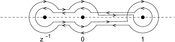
It is also possible to shrink the double loop in (5.4) and thus arrive at a sum of two classical Euler type integrals. For convenience assume that z<0z<0 and deform the double loop such that it consists of segments [z−1+ε,−ε][z^{-1}+\varepsilon,-\varepsilon], [ε,1−ε][\varepsilon,1-\varepsilon], circles of radius ε\varepsilon around z−1z^{-1} and 1, and two half circles of radius ε\varepsilon around 00, where each part is traversed various times and in different directions (see Figure 3). In Table 1 we list the arguments of the factors in the integrand for tt on the various parts of the double loop.
Refer to caption
Figure 3: Double loop prepared for shrinking in the integral in (5.4).
(0,1)⟶\genfrac{}{}{0.0pt}{}{(0,1)}{\longrightarrow} (0,1)⟵\genfrac{}{}{0.0pt}{}{(0,1)}{\longleftarrow} (z−1,0)⟵\genfrac{}{}{0.0pt}{}{(z^{-1},0)}{\longleftarrow} (z−1,0)⟶\genfrac{}{}{0.0pt}{}{(z^{-1},0)}{\longrightarrow} (0,1)⟶\genfrac{}{}{0.0pt}{}{(0,1)}{\longrightarrow} (0,1)⟵\genfrac{}{}{0.0pt}{}{(0,1)}{\longleftarrow} (z−1,0)⟵\genfrac{}{}{0.0pt}{}{(z^{-1},0)}{\longleftarrow} (z−1,0)⟶\genfrac{}{}{0.0pt}{}{(z^{-1},0)}{\longrightarrow}
arg⁡(t)\arg(t) 0 0 π\pi π\pi 2​π2\pi 2​π2\pi π\pi π\pi
arg⁡(1−t)\arg(1-t) 0 2​π2\pi 2​π2\pi 2​π2\pi 2​π2\pi 0 0 0
arg⁡(1−t​z)\arg(1-tz) 0 0 0 2​π2\pi 2​π2\pi 2​π2\pi 2​π2\pi 0
Table 1: Essential data while tt goes through the double loop.

Also assume that Re⁡a<1\operatorname{Re}a<1 and Re⁡c>Re⁡b>0\operatorname{Re}c>\operatorname{Re}b>0 with b−a,c−b∉ℤb-a,c-b\notin\mathbb{Z}, c∉ℤ≤0c\notin\mathbb{Z}_{\leq 0}. Then, as ε↓0\varepsilon\downarrow 0, the right-hand side of (5.4) tends to

Γ⁡(c)Γ⁡(b)​Γ​(c−b)​(∫01tb−1​(1−t)c−b−1​(1−t​z)−a​𝑑tCLOSE\displaystyle\frac{\Gamma(c)}{\Gamma(b)\Gamma(c-b)}\left(\int_{0}^{1}t^{b-1}(1-t)^{c-b-1}(1-tz)^{-a}\,dt\right.
−sin⁡(π​a)sin⁡(π⁡(a−b))∫z−10(−t)b−1(1−t)c−b−1(1−tz)−adt)\displaystyle\qquad\qquad\qquad\qquad\left.-\,\frac{\sin(\pi a)}{\sin(\pi(a-b))}\int_{z^{-1}}^{0}(-t)^{b-1}(1-t)^{c-b-1}(1-tz)^{-a}\,dt\right)
=2​F1​(a,bc,z)−Γ⁡(c)​Γ​(a−b)​Γ​(b−a+1)Γ⁡(b)​Γ​(c−b)​Γ​(a)​Γ​(1−a)​(−z)−b​∫01sb−1​(1−s)−a​(1−z−1​s)c−b−1​𝑑s\displaystyle=\,\mbox{}_{2}F_{1}\left(\genfrac{}{}{0.0pt}{}{a,b}{c};z\right)-\,\frac{\Gamma(c)\Gamma(a-b)\Gamma(b-a+1)}{\Gamma(b)\Gamma(c-b)\Gamma(a)\Gamma(1-a)}\,(-z)^{-b}\int_{0}^{1}s^{b-1}(1-s)^{-a}(1-z^{-1}s)^{c-b-1}\,ds
=2​F1​(a,bc,z)−Γ⁡(c)​Γ​(a−b)Γ⁡(a)​Γ​(c−b)​(−z)−b​2​F1​(b,b−c+1b−a+1,z−1),\displaystyle=\,\mbox{}_{2}F_{1}\left(\genfrac{}{}{0.0pt}{}{a,b}{c};z\right)-\,\frac{\Gamma(c)\Gamma(a-b)}{\Gamma(a)\Gamma(c-b)}\,(-z)^{-b}\,\mbox{}_{2}F_{1}\left(\genfrac{}{}{0.0pt}{}{b,b-c+1}{b-a+1};z^{-1}\right), (5.5)

where we used (2.2) and [9, 1.2(6)]. It follows that (5.5) is equal to (5.4), by which we have recovered [9, 2.10(2)].

Remark 5.1.

In the homological approach it is quite standard to prove connection formulas as above. See for instance Mimachi [18] for the more general case dealing with F23{}_{3}F_{2}.

5.2 A classical analysis version of Kita’s integral for H2H_{2}

We start with another corollary to Theorem 4.1.

Corollary 5.2.

For Re⁡a,Re⁡d,Re⁡(a+c),Re⁡(a+d),Re⁡(e−a−d)>0\operatorname{Re}a,\operatorname{Re}d,\operatorname{Re}(a+c),\operatorname{Re}(a+d),\operatorname{Re}(e-a-d)>0 and (x,y)∈ℂ2(x,y)\in\mathbb{C}^{2} such that x∉[1,∞)x\notin[1,\infty) and y∉[0,∞)y\notin[0,\infty), we have

Γ⁡(a+c)​Γ​(a+d)Γ⁡(a+c+d)​Γ​(a)​(−y)−c​FP​(a+c,b,c,e,c−d+1,x,−y−1)=Γ⁡(e)Γ⁡(e−a−d)​Γ​(a)​Γ​(d)\displaystyle\frac{\Gamma(a+c)\Gamma(a+d)}{\Gamma(a+c+d)\Gamma(a)}\,(-y)^{-c}F_{P}(a+c,b,c,e,c-d+1;x,-y^{-1})=\frac{\Gamma(e)}{\Gamma(e-a-d)\Gamma(a)\Gamma(d)}
×∫01∫01ua−1​(1−u)e−a−1​vd−1​(1−v)e−a−d−1​(1−u​x)−b​(1−(1−u)​u−1​v​y)−c​𝑑u​𝑑v\displaystyle\quad\times\int_{0}^{1}\int_{0}^{1}u^{a-1}(1-u)^{e-a-1}v^{d-1}(1-v)^{e-a-d-1}(1-ux)^{-b}\big(1-(1-u)u^{-1}vy\big)^{-c}\,du\,dv (5.6)
=Γ⁡(e)Γ⁡(e−a−d)​Γ​(a)​Γ​(d)​∫u=01∫v=0u−1−1ua+d−1​(1−u​x)−b​vd−1​(1−v​y)−c\displaystyle\qquad=\frac{\Gamma(e)}{\Gamma(e-a-d)\Gamma(a)\Gamma(d)}\,\int_{u=0}^{1}\int_{v=0}^{u^{-1}-1}u^{a+d-1}(1-ux)^{-b}v^{d-1}(1-vy)^{-c}
×(1−u−u​v)e−a−d−1​d​v​d​u\displaystyle\hskip 256.0748pt\times(1-u-uv)^{e-a-d-1}\,dv\,du (5.7)
=Γ⁡(e)Γ⁡(e−a−d)​Γ​(a)​Γ​(d)​∫u=01∫v=01−uua−1​(1−u​x)−b​vd−1​(1−u−1​v​y)−c\displaystyle\qquad=\frac{\Gamma(e)}{\Gamma(e-a-d)\Gamma(a)\Gamma(d)}\,\int_{u=0}^{1}\int_{v=0}^{1-u}u^{a-1}(1-ux)^{-b}v^{d-1}(1-u^{-1}vy)^{-c}
×(1−u−v)e−a−d−1​d​v​d​u.\displaystyle\hskip 256.0748pt\times(1-u-v)^{e-a-d-1}\,dv\,du. (5.8)

Proof. Formula (5.6) is a trivial rewriting of (4.6). We went from (5.6) to (5.7) by transforming (u,v)↦(u,u​v1−u)(u,v)\mapsto\big(u,\frac{uv}{1-u}\big) and from (5.7) to (5.8) by (u,v)↦(u,u−1​v)(u,v)\mapsto(u,u^{-1}v).∎
Expression (5.7) was evaluated as H2​(a,b,c,d,e,x,y)H_{2}(a,b,c,d,e;x,y) by Yoshida22 2 In [25, (0.10)] a power of −(u​v+u−1)-(uv+u-1) should be taken, because the integral is over a region with u​v+u−1≤0uv+u-1\leq 0. [25, (0.10)]. Kita [16, p.57, item 9] gave the same evaluation33 3 In [16, p.57, item 9] the second occurrence of z1z_{1} should be z2z_{2}. Also, on [16, p.27, line 3] the denominator Γ⁡(c)\Gamma(c) should be Γ⁡(γ)\Gamma(\gamma). for (5.8) as Yoshida gave for (5.7), but he specified that integration should be understood by the homological approach, which changes things drastically. Dwork & Loeser [8, p.105] also reproduce Yoshida’s formula, but without specification of the type of integral.

We will now show that we can reproduce Kita’s evaluation of (5.8) as H2H_{2} by working with classical integrals. For our purpose it is easier to work with a variant of the right-hand side of (5.6).

Theorem 5.3.

Let Re⁡d,Re⁡(e−a−d)>0\operatorname{Re}d,\operatorname{Re}(e-a-d)>0 and a,e−a∉ℤa,e-a\notin\mathbb{Z}. Then

H2(a,b,c,d;e,x,y)=Γ⁡(e)Γ⁡(e−a−d)​Γ​(a)​Γ​(d)1(1−e2​π​i​a)​(1−e2​π​i​(e−a))∫(1+,0+,1−,0−)×ua−1​(1−u)e−a−1​(1−u​x)−b​(∫01vd−1​(1−v)e−a−d−1​(1−(u−1−1)​v​y)−c​𝑑v)​𝑑u.H_{2}(a,b,c,d;e,x,y)=\frac{\Gamma(e)}{\Gamma(e-a-d)\Gamma(a)\Gamma(d)}\,\frac{1}{(1-e^{2\pi ia})(1-e^{2\pi i(e-a)})}\int^{(1+,0+,1-,0-)}\\ \times u^{a-1}(1-u)^{e-a-1}(1-ux)^{-b}\left(\int_{0}^{1}v^{d-1}(1-v)^{e-a-d-1}\big(1-(u^{-1}-1)vy\big)^{-c}\,dv\right)du. (5.9)

Here (x,y)∈ℂ2(x,y)\in\mathbb{C}^{2} and the double loop are such that u​x∉[1,∞)ux\notin[1,\infty) and (u−1−1)​y∉[1,∞)(u^{-1}-1)y\notin[1,\infty) for uu on the double loop.

Proof First choose x∈ℂx\in\mathbb{C} with |x|<1|x|<1. Then choose a double loop (1+,0+,1−,0−)(1+,0+,1-,0-) (as defined in the beginning of Section 5.1) such that x−1x^{-1} is not on the double loop and can be connected with ∞\infty without crossing the double loop. Then ua−1​(1−u)e−a−1​(1−u​x)−bu^{a-1}(1-u)^{e-a-1}(1-ux)^{-b} is well defined on the loop. Since the set {(u−1−1)v∣u∈(1+,0+,1−,0−),v∈[0,1]}\{(u^{-1}-1)v\mid u\in(1+,0+,1-,0-),\;v\in[0,1]\} is compact, we will have |(u−1−1)​v​y|<1|(u^{-1}-1)vy|<1 in the double integral (5.9) for |y||y| small enough. Thus, for such x,yx,y, the whole integrand is well defined, and so is the double integral.

Write the right-hand side of (5.9) as

Γ⁡(e)Γ⁡(e−a−d)​Γ​(a)​Γ​(d)​J.\frac{\Gamma(e)}{\Gamma(e-a-d)\Gamma(a)\Gamma(d)}\,J.

.In JJ we can expand (1−u​x)−b(1-ux)^{-b} and (1−(1−u)​u−1​v​y)−c\big(1-(1-u)u^{-1}vy\big)^{-c} as binomial series and interchange the double sum with the double integral by dominated convergence. We obtain that

J\displaystyle J =∑k,l=0∞(b)k​(c)lk!​l!​xk​yl​∫01vd+l−1​(1−v)e−a−d−1​𝑑v​∫(1+,0+,1−,0−)ua+k−l−1​(1−u)e−a+l−1​𝑑u\displaystyle=\sum_{k,l=0}^{\infty}\frac{(b)_{k}(c)_{l}}{k!\,l!}\,x^{k}y^{l}\,\int_{0}^{1}v^{d+l-1}(1-v)^{e-a-d-1}\,dv\int^{(1+,0+,1-,0-)}u^{a+k-l-1}(1-u)^{e-a+l-1}\,du
=∑k,l=0∞(a)k−l​(b)k​(c)l​(d)l(e)k​k!​l!​xk​yl=H2​(a,b,c,d,e,x,y).\displaystyle=\sum_{k,l=0}^{\infty}\frac{(a)_{k-l}(b)_{k}(c)_{l}(d)_{l}}{(e)_{k}k!\,l!}\,x^{k}y^{l}=H_{2}(a,b,c,d,e;x,y).

Analytic continuation in xx and yy with simultaneous deformation of the double loop is possible as long as u​x∉[1,∞)ux\notin[1,\infty) and (u−1−1)​y∉[1,∞)(u^{-1}-1)y\notin[1,\infty) for uu on the double loop.∎

5.3 The integral (5.9) as a solution of the F2F_{2} system and analytic continuation

We can rewrite (5.9) as

y−b2​H2​(a−b2,b1,b2,b2−c2+1,c1,x,−y−1)=Γ⁡(c1)Γ⁡(−a+c1+c2−1)​Γ​(a−b2)​Γ​(b2−c2+1)\displaystyle y^{-b_{2}}H_{2}(a-b_{2},b_{1},b_{2},b_{2}-c_{2}+1,c_{1};x,-y^{-1})=\frac{\Gamma(c_{1})}{\Gamma(-a+c_{1}+c_{2}-1)\Gamma(a-b_{2})\Gamma(b_{2}-c_{2}+1)}
×y−b2(1−e2​π​i​(a−b2))​(1−e2​π​i​(−a+b2+c1))​∫(1+,0+,1−,0−)ua−b2−1​(1−u)−a+b2+c1−1​(1−x​u)−b1\displaystyle\times\frac{y^{-b_{2}}}{(1-e^{2\pi i(a-b_{2})})(1-e^{2\pi i(-a+b_{2}+c_{1})})}\,\int^{(1+,0+,1-,0-)}u^{a-b_{2}-1}(1-u)^{-a+b_{2}+c_{1}-1}(1-xu)^{-b_{1}}
×(∫01vb2−c2​(1−v)−a+c1+c2−2​(1−y−1​(1−u−1)​v)−b2​𝑑v)​𝑑u=:I⁡(x,y),\displaystyle\qquad\qquad\quad\times\left(\int_{0}^{1}v^{b_{2}-c_{2}}(1-v)^{-a+c_{1}+c_{2}-2}\big(1-y^{-1}(1-u^{-1})v\big)^{-b_{2}}\,dv\right)du=:I(x,y), (5.10)

where Re⁡(b2−c1+1),Re⁡(−a+c1+c2−1)>0\operatorname{Re}(b_{2}-c_{1}+1),\operatorname{Re}(-a+c_{1}+c_{2}-1)>0 and a−b2,−a+b2+c1∉ℤa-b_{2},-a+b_{2}+c_{1}\notin\mathbb{Z}, while |x|<1|x|<1 and |y||y| is large enough, with the same branch choice for the two occurrences of y−b2y^{-b_{2}}. By [21, (14)] the left-hand side of (5.10) is a solution of the system [9, 5.9(10)] of pde’s for F2F_{2}. Actually, see also (3.1), it is the unique solution of this system of the form y−b2​∑i,j=0∞ci,j​xi​y−jy^{-b_{2}}\sum_{i,j=0}^{\infty}c_{i,j}x^{i}y^{-j} with c0,0=1c_{0,0}=1 which is analytic in a neigbourhood of (x,y)=(0,∞)(x,y)=(0,\infty).

The singular loci of the F2F_{2} system are the points around which the local solution space has dimension less than the generic dimension four. It is well known (and easily derived) that the singular loci are the lines x=0x=0, x=1x=1, y=0y=0, y=1y=1, x+y=1x+y=1 and (after one-point compactification of the two ℂ\mathbb{C}-factors of ℂ2\mathbb{C}^{2}) x=∞x=\infty, y=∞y=\infty. We conclude that the left-hand side of (5.10) can be certainly analytically extended to a one-valued analytic function on the regions in ℝ2\mathbb{R}^{2} given by y>1y>1, 1−y<x<11-y<x<1 and by x<1x<1, y<0y<0. We will show that this can also be read off from the right-hand side I⁡(x,y)I(x,y) of (5.10).

First we evaluate the inner integral in I⁡(x,y)I(x,y) as an Euler integral (2.2):

I⁡(x,y)=Γ⁡(c1)Γ⁡(a−b2)​Γ​(−a+b2+c1)​y−b2(1−e2​π​i​(a−b2))​(1−e2​π​i​(−a+b2+c1))\displaystyle I(x,y)=\frac{\Gamma(c_{1})}{\Gamma(a-b_{2})\Gamma(-a+b_{2}+c_{1})}\,\frac{y^{-b_{2}}}{(1-e^{2\pi i(a-b_{2})})(1-e^{2\pi i(-a+b_{2}+c_{1})})}
×∫(1+,0+,1−,0−)ua−b2−1​(1−u)−a+b2+c1−1​(1−x​u)−b1​2​F1​(b2,b2−c2+1−a+b2+c1,y−1​(1−u−1))​𝑑u.\displaystyle\times\int^{(1+,0+,1-,0-)}u^{a-b_{2}-1}(1-u)^{-a+b_{2}+c_{1}-1}(1-xu)^{-b_{1}}\,\mbox{}_{2}F_{1}\left(\genfrac{}{}{0.0pt}{}{b_2,b_2-c_2+1}{-a+b_2+c_1};y^{-1}(1-u^{-1})\right)\,du. (5.11)

Then the constraints Re⁡(b2−c1+1),Re⁡(−a+c1+c2−1)>0\operatorname{Re}(b_{2}-c_{1}+1),\operatorname{Re}(-a+c_{1}+c_{2}-1)>0 for (5.10) can be dropped, while the other constraints are still kept. For analytic continuation in (5.11) we can simultaneously bring (x,y)(x,y) to a larger region and deform the double loop. We will certainly have a one-valued analytic continuation as long as, for uu in the double loop, x​uxu and y−1​(1−u−1)y^{-1}(1-u^{-1}) do not cross the cut [1,∞)[1,\infty). For (x,y)∈ℝ2(x,y)\in\mathbb{R}^{2} and in the mentioned domains y>1y>1, 1−y<x<11-y<x<1 or x<1x<1, y<0y<0 of unique analytic continuation for y−b2​H2​(x,−y−1)y^{-b_{2}}H_{2}(x,-y^{-1}) we distinghuish four cases. We will see that in each case the two cuts are no obstruction for the double loop.

  1. 1.

    x≤0x\leq 0 and x+y>1x+y>1. Then uu has to remain outside (−∞,x−1](-\infty,x^{-1}] and [(1−y)−1,0][(1-y)^{-1},0], so uu can pass ℝ\mathbb{R} through the holes (1,∞)(1,\infty) and (x−1,(1−y)−1)(x^{-1},(1-y)^{-1}) (left from 0).

  2. 2.

    0≤x<10\leq x<1 and y>1y>1. Then uu has to remain outside [(1−y)−1,0][(1-y)^{-1},0] and [x−1,∞)[x^{-1},\infty), so uu can pass ℝ\mathbb{R} through the holes (1,x−1)(1,x^{-1}) and (−∞,(1−y)−1)(-\infty,(1-y)^{-1}) (left from 0).

  3. 3.

    x≤0x\leq 0 and y<0y<0. Then uu has to remain outside (−∞,x−1](-\infty,x^{-1}] and [0,(1−y)−1][0,(1-y)^{-1}], so uu can pass ℝ\mathbb{R} through the holes (1,∞)(1,\infty) and (x−1,0)(x^{-1},0).

  4. 4.

    0≤x<10\leq x<1 and y<0y<0. Then uu has to remain outside [0,(1−y)−1][0,(1-y)^{-1}] and [x−1,∞)[x^{-1},\infty), so uu can pass ℝ\mathbb{R} through the holes (1,x−1)(1,x^{-1}) and (−∞,0)(-\infty,0).

In a way depending on the case the double loop can be next shrunk, analogous to our treatment of (5.4). As an illustration we will only treat the first case.

5.4 Shrinking the double loop in (5.11)

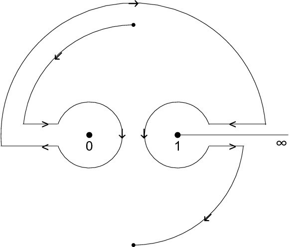
We will continue with case 1 above. Assume that x<0x<0 and x+y>1x+y>1. Deform the double loop in (5.11) such that it consists of segments [(1−y)−1+ε,−ε][(1-y)^{-1}+\varepsilon,-\varepsilon], [ε,1−ε][\varepsilon,1-\varepsilon], circles of radius ε\varepsilon around (1−y)−1(1-y)^{-1} and 1, and half circles of radius ε\varepsilon around 0, where each part is traversed various times and in different directions (see Figure 4). One has to do good bookkeeping of the arguments of uu, 1−u1-u and y−1​(1−u−1)y^{-1}(1-u^{-1}) while uu goes through the double loop, since these will affect the integrand. See Figure 5 for the orbit of (1−u−1)​y−1(1-u^{-1})y^{-1} while uu goes through the double loop. See Table 2 for the essential data associated with the double loop.

Refer to caption
Figure 4: Double loop prepared for shrinking in the integral in (5.11).
Refer to caption
Refer to caption

4

Figure 5: Orbits of (1−u−1)​y−1(1-u^{-1})y^{-1} during the first and second part of the double loop.
(0,1)⟶\genfrac{}{}{0.0pt}{}{(0,1)}{\longrightarrow} (0,1)⟵\genfrac{}{}{0.0pt}{}{(0,1)}{\longleftarrow} ((1−y)−1,0)+i​0⟵\genfrac{}{}{0.0pt}{}{((1-y)^{-1},0)+i0}{\longleftarrow} ((1−y)−1,0)−i​0⟶\genfrac{}{}{0.0pt}{}{((1-y)^{-1},0)-i0}{\longrightarrow}
arg⁡(u)=\arg(u)= 0 0 π\pi π\pi
arg⁡(1−u)=\arg(1-u)= 0 2​π2\pi 2​π2\pi 2​π2\pi
(1−u−1)​y−1∈(1-u^{-1})y^{-1}\in (−∞,0)(-\infty,0) (−∞,0)(-\infty,0) (1,∞)+i​0(1,\infty)+i0 (1,∞)−i​0(1,\infty)-i0
(0,1)⟶\genfrac{}{}{0.0pt}{}{(0,1)}{\longrightarrow} (0,1)⟵\genfrac{}{}{0.0pt}{}{(0,1)}{\longleftarrow} ((1−y)−1,0)−i​0⟵\genfrac{}{}{0.0pt}{}{((1-y)^{-1},0)-i0}{\longleftarrow} ((1−y)−1,0)+i​0⟶\genfrac{}{}{0.0pt}{}{((1-y)^{-1},0)+i0}{\longrightarrow}
arg⁡(u)=\arg(u)= 2​π2\pi 2​π2\pi π\pi π\pi
arg⁡(1−u)=\arg(1-u)= 2​π2\pi 0 0 0
(1−u−1)​y−1∈(1-u^{-1})y^{-1}\in (−∞,0)(-\infty,0) (−∞,0)(-\infty,0) (1,∞)−i​0(1,\infty)-i0 (1,∞)+i​0(1,\infty)+i0
Table 2: Essential data while uu goes through the double loop.

We already had the constraints a−b2,−a+b2+c1∉ℤa-b_{2},-a+b_{2}+c_{1}\notin\mathbb{Z}. In order to allow the shrinking as ε↓0\varepsilon\downarrow 0 we also need the constraints

  • •

    at u=1u=1: Re⁡(b2+c1−a)>0\operatorname{Re}(b_{2}+c_{1}-a)>0;

  • •

    at u=0u=0: Re⁡a,Re⁡(a−c2+1)>0\operatorname{Re}a,\operatorname{Re}(a-c_{2}+1)>0 (use [9, 2.10(2)]);

  • •

    at u=(1−y)−1u=(1-y)^{-1}: Re⁡(−a−b1+c1+c2)>0\operatorname{Re}(-a-b_{1}+c_{1}+c_{2})>0 (use [9, 2.10(1)]).

In the limit for ε↓0\varepsilon\downarrow 0 there will result the sum of an integral over u∈[0,1]u\in[0,1] and an integral over u∈[(1−y)−1,0]u\in[(1-y)^{-1},0]. For both integrals we collect four instances of the integrand in (5.11) with branch choices following Table 2. These four instances are added, where a term has positive sign if the arrow in Table 2 is in forward direction, and negative sign for an arrow in negative direction. We obtain (also use [9, 1.2(6)]):

I⁡(x,y)=I1​(x,y)+I2​(x,y)I(x,y)=I_{1}(x,y)+I_{2}(x,y) (5.12)

with

I1​(x,y)=Γ⁡(c1)Γ⁡(a−b2)​Γ​(−a+b2+c1)​y−b2​∫01ua−b2−1​(1−u)−a+b2+c1−1​(1−x​u)−b1×2​F1​(b2,b2−c2+1−a+b2+c1,y−1​(1−u−1))​d​uI_{1}(x,y)=\frac{\Gamma(c_{1})}{\Gamma(a-b_{2})\Gamma(-a+b_{2}+c_{1})}\,y^{-b_{2}}\int_{0}^{1}u^{a-b_{2}-1}(1-u)^{-a+b_{2}+c_{1}-1}(1-xu)^{-b_{1}}\\ \times\,\mbox{}_{2}F_{1}\left(\genfrac{}{}{0.0pt}{}{b_2,b_2-c_2+1}{-a+b_2+c_1};y^{-1}(1-u^{-1})\right)\,du (5.13)

and

I2​(x,y)=Γ⁡(c1)​Γ​(−a+b2+1)Γ⁡(−a+b2+c1)​y−b22​π​i​∫(1−y)−10(−u)a−b2−1​(1−u)−a+b2+c1−1​(1−x​u)−b1×(2​F1​(b2,b2−c2+1−a+b2+c1,y−1​(1−u−1)+i​0)−2​F1​(b2,b2−c2+1−a+b2+c1,y−1​(1−u−1)−i​0))​d​u.I_{2}(x,y)=\frac{\Gamma(c_{1})\Gamma(-a+b_{2}+1)}{\Gamma(-a+b_{2}+c_{1})}\,\frac{y^{-b_{2}}}{2\pi i}\int_{(1-y)^{-1}}^{0}(-u)^{a-b_{2}-1}(1-u)^{-a+b_{2}+c_{1}-1}(1-xu)^{-b_{1}}\\ \times\left(\,\mbox{}_{2}F_{1}\left(\genfrac{}{}{0.0pt}{}{b_2,b_2-c_2+1}{-a+b_2+c_1};y^{-1}(1-u^{-1})+i0\right)-\,\mbox{}_{2}F_{1}\left(\genfrac{}{}{0.0pt}{}{b_2,b_2-c_2+1}{-a+b_2+c_1};y^{-1}(1-u^{-1})-i0\right)\right)du. (5.14)

In (5.13) we can relax the parameter constraints to those given above at u=0u=0 and u=1u=1. By (4.7) we see that

I1​(x,y)=Γ⁡(a)​Γ​(a−c2+1)Γ⁡(a+b2−c2+1)​Γ​(a−b2)​FP​(a,b1,b2,c1,c2,x,y),I_{1}(x,y)=\frac{\Gamma(a)\Gamma(a-c_{2}+1)}{\Gamma(a+b_{2}-c_{2}+1)\Gamma(a-b_{2})}\,F_{P}(a,b_{1},b_{2},c_{1},c_{2};x,y), (5.15)

In (5.14) we can write the difference of the two F12{}_{2}F_{1} as one F12{}_{2}F_{1} in view of [9, 2.10(1)], and next apply Euler’s transformation (2.6):

12​π​i​(2​F1​(a,bc,x+i​0)−2​F1​(a,bc,x−i​0))\displaystyle\frac{1}{2\pi i}\left(\,\mbox{}_{2}F_{1}\left(\genfrac{}{}{0.0pt}{}{a,b}{c};x+i0\right)-\,\mbox{}_{2}F_{1}\left(\genfrac{}{}{0.0pt}{}{a,b}{c};x-i0\right)\right)
=Γ⁡(c)Γ⁡(a)​Γ​(b)​Γ​(c−a−b+1)​(x−1)c−a−b​2​F1​(c−a,c−bc−a−b+1,1−x)\displaystyle\qquad=\frac{\Gamma(c)}{\Gamma(a)\Gamma(b)\Gamma(c-a-b+1)}\,(x-1)^{c-a-b}\,\,\mbox{}_{2}F_{1}\left(\genfrac{}{}{0.0pt}{}{c-a,c-b}{c-a-b+1};1-x\right)
=Γ⁡(c)Γ⁡(a)​Γ​(b)​Γ​(c−a−b+1)x1−c(x−1)c−a−b2F1(1−a,1−bc−a−b+1;1−x)(x∈(1,∞)).\displaystyle\qquad=\frac{\Gamma(c)}{\Gamma(a)\Gamma(b)\Gamma(c-a-b+1)}\,x^{1-c}(x-1)^{c-a-b}\,\,\mbox{}_{2}F_{1}\left(\genfrac{}{}{0.0pt}{}{1-a,1-b}{c-a-b+1};1-x\right)\quad(x\in(1,\infty)).

Then (5.14) takes the form

I2​(x,y)=Γ⁡(c1)​Γ​(b2−a+1)Γ⁡(b2)​Γ​(b2−c2+1)​Γ​(c1+c2−a−b2)​yb2−c2​∫(1−y)−10(−u)a+b2−c2−1\displaystyle I_{2}(x,y)=\frac{\Gamma(c_{1})\Gamma(b_{2}-a+1)}{\Gamma(b_{2})\Gamma(b_{2}-c_{2}+1)\Gamma(c_{1}+c_{2}-a-b_{2})}\,y^{b_{2}-c_{2}}\int_{(1-y)^{-1}}^{0}(-u)^{a+b_{2}-c_{2}-1}
×(1+u⁡(y−1))c1+c2−a−b2−1​(1−x​u)−b1​2​F1​(c2−b2,1−b2c1+c2−a−b2,1−y−1​(1−u−1))​d​u\displaystyle\quad\times\big(1+u(y-1)\big)^{c_{1}+c_{2}-a-b_{2}-1}(1-xu)^{-b_{1}}\,\mbox{}_{2}F_{1}\left(\genfrac{}{}{0.0pt}{}{c_2-b_2,1-b_2}{c_1+c_2-a-b_2};1-y^{-1}(1-u^{-1})\right)\,du
=Γ⁡(c1)​Γ​(b2−a+1)Γ⁡(b2)​Γ​(b2−c2+1)​Γ​(c1+c2−a−b2)​(y−1)−a​(yy−1)b2−c2​∫01wa+b2−c2−1\displaystyle=\frac{\Gamma(c_{1})\Gamma(b_{2}-a+1)}{\Gamma(b_{2})\Gamma(b_{2}-c_{2}+1)\Gamma(c_{1}+c_{2}-a-b_{2})}\,(y-1)^{-a}\left(\frac{y}{y-1}\right)^{b_{2}-c_{2}}\int_{0}^{1}w^{a+b_{2}-c_{2}-1}
×(1−w)c1+c2−a−b2−1​(1−x​w1−y)−b1​2​F1​(c2−b2,1−b2c1+c2−a−b2,y−1y​(1−w−1))​d​w\displaystyle\quad\times(1-w)^{c_{1}+c_{2}-a-b_{2}-1}\left(1-\frac{xw}{1-y}\right)^{-b_{1}}\,\mbox{}_{2}F_{1}\left(\genfrac{}{}{0.0pt}{}{c_2-b_2,1-b_2}{c_1+c_2-a-b_2};\frac{y-1}{y}(1-w^{-1})\right)\,dw
=Γ⁡(b2−a+1)​Γ​(a)​Γ​(a−c2+1)Γ⁡(b2)​Γ​(a−b2+1)​Γ​(b2−c2+1)​(y−1)−a​FP​(a,b1,c2−b2,c1,c2,x1−y,yy−1).\displaystyle=\frac{\Gamma(b_{2}-a+1)\Gamma(a)\Gamma(a-c_{2}+1)}{\Gamma(b_{2})\Gamma(a-b_{2}+1)\Gamma(b_{2}-c_{2}+1)}\,(y-1)^{-a}\,F_{P}\left(a,b_{1},c_{2}-b_{2},c_{1},c_{2};\frac{x}{1-y},\frac{y}{y-1}\right). (5.16)

Here we have made the change of integration variable u=w​(1−y)−1u=w(1-y)^{-1} in the second equality, and we have used (4.7) in the third equality. Furthermore, we can relax in (5.16) the parameter constraints to those given above at u=0u=0 and u=(1−y)−1u=(1-y)^{-1}. These are in agreement with the parameter constraints in (4.7) (with b2b_{2} replaced by c2−b2c_{2}-b_{2}).

Remark 5.4.

The identity (5.12) with (5.10), (5.13), (5.16) substituted agrees with Olsson’s identity [21, (53)].

Remark 5.5.

If in the present section from (5.11) until here we make the specializations x=0x=0, c1=ac_{1}=a then the F12{}_{2}F_{1} in (5.11) specializes to (1−y−1​(1−u−1))c2−b2−1\big(1-y^{-1}(1-u^{-1})\big)^{c_{2}-b_{2}-1} by (2.7). The subsequent decomposition (5.12) (i.e., I⁡(0,y)=I1​(0,y)+I2​(0,y)I(0,y)=I_{1}(0,y)+I_{2}(0,y)) gives then another example of what we wrote in Section 5.1 starting with (5.3). There results a formula connecting three Gauss hypergometric functions (also seen by applying (3.3) and (4.8) to (5.10) and (5.15), (5.16), respectively) which is essentially the connection formula [9, 2.10(3)].

Remark 5.6.

Kato [15] also discusses the solutions of the F2F_{2} system at the various singular points, but he does not refer to Olsson [21], and he gives, apart from F2F_{2}, few explicit solutions. However, the first double power series in his Remark on p.330 can be recognized as FP​(a,b2,b1,c2,c1,y,x)F_{P}(a,b_{2},b_{1},c_{2},c_{1};y,x) expanded as (4.4). The three solutions I⁡(x,y)I(x,y), I1​(x,y)I_{1}(x,y) and I2​(x,y)I_{2}(x,y) of the F2F_{2} system occurring above in (5.10), (5.15), (5.16), respectively, can be matched up to a constant factor with the following solutions in [15]: I1​(x,y)I_{1}(x,y) with the first solution in §3.2.1, I2​(x,y)I_{2}(x,y) with the first solution in §3.3.5, and I⁡(x,y)I(x,y) with the third solution in §3.3.5. Kato gives many connection formulas, but apparently not the one connecting II, I1I_{1} and I2I_{2}.

Remark 5.7.

Kita’s integral representations for Appell F2F_{2} and F3F_{3} [16, p.56, items 2.2 and 3], which go back to Hattori & Kimura [11], and where the double integral is defined by the homological approach, remain valid if the double integral is defined classically, but then further constraints on the parameters are needed. It would be interesting to consider also the other new double integral representations given by Yoshida [25, (0.6)–(0.9)], which come back in Kita [16] (for Yoshida’s alternative F2F_{2}-integral [25, (0.6)] see also Yoshida [26, p.71]). Are these easy cases like the double integrals for F2F_{2} and F3F_{3} or would their classical counterparts be a sum of two integral representations?

6 Double integrals for solutions of the F2F_{2} system

Olsson’s list [21, p.1289, Table I] of solutions of the system of PDEs [9, 5.9(10)] for F2F_{2} includes, besides F2F_{2} itself, for instance functions expressible in terms of F3F_{3}, of H2H_{2}, and of FPF_{P}. It is interesting to rewrite the well-known double integral representations44 4 In [9, 5.8(3)], in the exponent of (1−u−v)(1-u-v), one should replace −γ-\gamma by γ\gamma. [9, 5.8(2),(3)] for F2F_{2} and F3F_{3} and our double integral representations (3.6) for H2H_{2} and (4.6) for FPF_{P} as integral representations for solutions of the F2F_{2} system. We obtain:

F2​(a,b1,b2,c1,c2,x,y)=Γ⁡(c1)​Γ​(c2)Γ⁡(b1)​Γ​(b2)​Γ​(c1−b1)​Γ​(c2−b2)\displaystyle F_{2}(a,b_{1},b_{2},c_{1},c_{2};x,y)=\frac{\Gamma(c_{1})\Gamma(c_{2})}{\Gamma(b_{1})\Gamma(b_{2})\Gamma(c_{1}-b_{1})\Gamma(c_{2}-b_{2})}
×x1−c1​y1−c2​∫u=0x∫v=0yub1−1​vb2−1​(1−u−v)−a​(x−u)c1−b1−1​(y−v)c2−b2−1​𝑑v​𝑑u\displaystyle\qquad\times x^{1-c_{1}}y^{1-c_{2}}\int_{u=0}^{x}\int_{v=0}^{y}u^{b_{1}-1}v^{b_{2}-1}(1-u-v)^{-a}(x-u)^{c_{1}-b_{1}-1}(y-v)^{c_{2}-b_{2}-1}\,dv\,du
(0<x<1−y⁡<1,Re⁡b1,Re⁡b2,Re⁡(c1−b1),Re⁡(c2−b2)>​0),\displaystyle\qquad\qquad\qquad\qquad\qquad(0<x<1-y<1,\;\operatorname{Re}b_{1},\operatorname{Re}b_{2},\operatorname{Re}(c_{1}-b_{1}),\operatorname{Re}(c_{2}-b_{2})>0), (6.1)
x−b1​y−b2​F3​(b1,b2,1+b1−c1,1+b2−c2,b1+b2−a+1,x−1,y−1)=Γ⁡(b1+b2−a+1)Γ⁡(b1)​Γ​(b2)​Γ​(1−a)\displaystyle x^{-b_{1}}y^{-b_{2}}F_{3}(b_{1},b_{2},1+b_{1}-c_{1},1+b_{2}-c_{2},b_{1}+b_{2}-a+1;x^{-1},y^{-1})=\frac{\Gamma(b_{1}+b_{2}-a+1)}{\Gamma(b_{1})\Gamma(b_{2})\Gamma(1-a)}
×x1−c1​y1−c2​∫v=01∫u=01−vub1−1​vb2−1​(1−u−v)−a​(x−u)c1−b1−1​(y−v)c2−b2−1​𝑑u​𝑑v\displaystyle\qquad\qquad\times x^{1-c_{1}}y^{1-c_{2}}\int_{v=0}^{1}\int_{u=0}^{1-v}u^{b_{1}-1}v^{b_{2}-1}(1-u-v)^{-a}(x-u)^{c_{1}-b_{1}-1}(y-v)^{c_{2}-b_{2}-1}\,du\,dv
(x,y>1,Re⁡b1,Re⁡b2,Re⁡(1−a)>0),\displaystyle\qquad\qquad\qquad\qquad\qquad\qquad\qquad\qquad\qquad\qquad(x,y>1,\;\operatorname{Re}b_{1},\operatorname{Re}b_{2},\operatorname{Re}(1-a)>0), (6.2)
y−b2​H2​(a−b2,b1,b2−c2+1,b2,c1,x,−y−1)=Γ⁡(b2−a+1)​Γ​(c1)Γ⁡(1−a)​Γ​(b2)​Γ​(b1)​Γ​(c1−b1)​x1−c1​y1−c2\displaystyle y^{-b_{2}}H_{2}(a-b_{2},b_{1},b_{2}-c_{2}+1,b_{2},c_{1};x,-y^{-1})=\frac{\Gamma(b_{2}-a+1)\Gamma(c_{1})}{\Gamma(1-a)\Gamma(b_{2})\Gamma(b_{1})\Gamma(c_{1}-b_{1})}\,x^{1-c_{1}}y^{1-c_{2}}
×∫u=0x∫v=01−uub1−1​vb2−1​(1−u−v)−a​(x−u)c1−b1−1​(y−v)c2−b2−1​𝑑v​𝑑u\displaystyle\qquad\qquad\qquad\times\int_{u=0}^{x}\int_{v=0}^{1-u}u^{b_{1}-1}v^{b_{2}-1}(1-u-v)^{-a}(x-u)^{c_{1}-b_{1}-1}(y-v)^{c_{2}-b_{2}-1}\,dv\,du
(0​<x⁡<1,y>​1,Re⁡(1−a),Re⁡b2,Re⁡b1,Re⁡(c1−b1)>​0),\displaystyle\qquad\qquad\qquad\qquad\qquad(0<x<1,\;y>1,\;\operatorname{Re}(1-a),\operatorname{Re}b_{2},\operatorname{Re}b_{1},\operatorname{Re}(c_{1}-b_{1})>0), (6.3)
|x|1−c1​y1−c2​FP​(a−c1−c2+2,b1−c1+1,b2−c2+1,2−c1,2−c2,x,y)\displaystyle|x|^{1-c_{1}}y^{1-c_{2}}F_{P}(a-c_{1}-c_{2}+2,b_{1}-c_{1}+1,b_{2}-c_{2}+1,2-c_{1},2-c_{2};x,y)
=Γ⁡(a+b2−c1−c2+2)​Γ​(2−c1)Γ⁡(a−c1−c2+2)​Γ​(a−c1+1)​Γ​(b2)​Γ​(1−a)​|x|1−c1​y1−c2​∫u=1∞∫v=1−u0ub1−1​(−v)b2−1\displaystyle\quad=\frac{\Gamma(a+b_{2}-c_{1}-c_{2}+2)\Gamma(2-c_{1})}{\Gamma(a-c_{1}-c_{2}+2)\Gamma(a-c_{1}+1)\Gamma(b_{2})\Gamma(1-a)}\,|x|^{1-c_{1}}y^{1-c_{2}}\int_{u=1}^{\infty}\int_{v=1-u}^{0}u^{b_{1}-1}(-v)^{b_{2}-1}
×(u+v−1)−a​(u−x)c1−b1−1​(y−v)c2−b2−1​d​v​d​u(x∈(−∞,0)∪(0,1),y>0CLOSE;\displaystyle\qquad\times(u+v-1)^{-a}(u-x)^{c_{1}-b_{1}-1}(y-v)^{c_{2}-b_{2}-1}\,dv\,du\quad\big(x\in(-\infty,0)\cup(0,1),y>0;
OPENRe⁡a<1,Re⁡b2>0,Re⁡(a−c1−c2+2),Re⁡(a−c1+1),Re⁡b2,Re⁡(1−a)>0).\displaystyle\qquad\quad\operatorname{Re}a<1,\;\operatorname{Re}b_{2}>0,\;\operatorname{Re}(a-c_{1}-c_{2}+2),\operatorname{Re}(a-c_{1}+1),\operatorname{Re}b_{2},\operatorname{Re}(1-a)>0\big). (6.4)

Here we have restricted to domains of (x,y)(x,y) in ℝ2\mathbb{R}^{2}. For going from (4.6) to (6.4) make the change of integration variables (u,v)→(u−1,v/(1−u))(u,v)\to(u^{-1},v/(1-u)).

Note that the right-hand sides of (6.1)–(6.4) all have the form

const.|x|1−c1​|y|1−c2​∫∫|u|b1−1​|v|b2−1​|1−u−v|−a​|x−u|c1−b1−1​|y−v|c2−b2−1​𝑑v​𝑑u,{\rm const.}\,|x|^{1-c_{1}}|y|^{1-c_{2}}\int\!\!\int|u|^{b_{1}-1}|v|^{b_{2}-1}|1-u-v|^{-a}|x-u|^{c_{1}-b_{1}-1}|y-v|^{c_{2}-b_{2}-1}\,dv\,du,

where the integral is over a suitable (u,v)(u,v) region. This will enable uniform proofs of such identities by showing that the right-hand sides are solutions of the system of pde’s for F2F_{2}, quite similar as was done in [17] in the one-variable case. In Chapter 6 of the PhD Thesis by the first author55 5 E. Diekema, The fractional orthogonal derivative for functions of one and two variables, PhD Thesis, University of Amsterdam, 2018; http://hdl.handle.net/11245.1/a6ed8a3f-0831-4f9a-9476-2661ec7e1f92 the double integrals (6.1)–(6.3) appear as integral kernels in certain approximations of two-dimensional fractional integrals.

Acknowledgements

The authors are very grateful to the referees. Their thoughtful comments about an earlier version of Section 5 (The Yoshida-Kita integral for H2H_{2}) helped us greatly to do a complete rewriting and extension of this section, providing a much deeper insight about the relationship between the Yoshida-Kita integral for H2H_{2} on the one hand and our double integral for FPF_{P} on the other. Comments about the subsequent version indicated an annoying error and led to a shortening of the proof of (5.16). Many smaller details could also be improved and important references could be added as a result of these comments.

References

  • [1] H. Almström and P. Olsson, Analytic properties of certain radial matrix elements, J. Math. Phys. 8 (1967), 2013–2021.
  • [2] G. E. Andrews, R. Askey and R. Roy, Special functions, Cambridge University Press, 1999.
  • [3] K. Aomoto and M. Kita, Theory of hypergeometric functions, Springer-Verlag, 2011.
  • [4] P. Appell, Sur les se´\acute{e}ries hypergéométriques de deux variables et sur des équations différentielles linéaires aux dérivées partielles, C. R. Acad. Sci. Paris 90 (1880), 296–298.
  • [5] P. Appell, Sur les fonctions hypergéométriques de deux variables, J. Math. Pures Appl. (3) 8 (1882), 173–216.
  • [6] P. Appell and M. J. Kampé de Fériet, Fonctions hypergéométriques et hypersphériques. Polynômes d’Hermite, Gauthier-Villars, 1926.
  • [7] W. N. Bailey, Generalized hypergeometric series, Cambridge University Press, 1935.
  • [8] B. Dwork and F. Loeser, Hypergeometric series, Japan. J. Math. 19 (1993), 81–129.
  • [9] A. Erdélyi, Higher transcendental functions, Vol. I, McGraw-Hill, 1953.
  • [10] H. Exton, Multiple hypergeometric functions and applications, Ellis Horwood, 1976.
  • [11] A. Hattori and T. Kimura, On the Euler integral representations of hypergeometric functions in several variables, J. Math. Soc. Japan 26 (1974), 1–16.
  • [12] J. Horn, Ueber die Convergenz der Hypergeometrische Reihen Zweier und Dreier Veränderlichen, Math. Ann. 34 (1889), 544–600.
  • [13] J. Horn, Hypergeometrische Funktionen Zweier Veränderlichen, Math. Ann. 105 (1931), 381–407.
  • [14] C. Jordan, Cours d’analyse de l’École Polytechnique, Tome III, Gauthier-Villars, Paris, 1887.
  • [15] M. Kato, Connection formulas and irreducibility conditions for Appell’s F2F_{2}, Kyushu J. Math. 66 (2012), 325–363.
  • [16] M. Kita, On hypergeometric functions in several variables, Japan. J. Math. 18 (1992), 25–74.
  • [17] T. H. Koornwinder, Fractional integral and generalized Stieltjes transforms for hypergeometric functions as transmutation operators, SIGMA 11 (2015), 074; arXiv:1504.08144.
  • [18] K. Mimachi, Connection matrices associated with the generalized hypergeometric function F23{}_{3}F_{2}, Funkcial. Ekvac. 51 (2008), 107–133.
  • [19] P. O. M. Olsson, The Laplace transform of a product of two Whittaker functions, Ark. Fys. B28 (1965), 113–120.
  • [20] P. O. M. Olsson, A hypergeometric function of two variables of importance in perturbation theory. I, Ark. Fys. B30 (1965), 187–191.
  • [21] P. O. M. Olsson, On the integration of the differential equations of five-parametric double hypergeometric functions of second order, J. Math. Phys. 18 (1977), 1285–1294.
  • [22] L. Pochhammer, Zur Theorie der Euler’schen Integrale, Math. Ann. 35 (1890), 495–526.
  • [23] L. J. Slater, Generalized hypergeometric functions, Cambridge University Press, 1966.
  • [24] V. K. Tuan and S. I. Kalla, Some transformations and integral representations of Horn’s functions, Rev. Técn. Fac. Ingr. Univ. Zulia 10 (1987), 81–94.
  • [25] M. Yoshida, Euler integral transformations of hypergeometric functions of two variables, Hiroshima Math. J. 10 (1980), 329–335.
  • [26] M. Yoshida, Fuchsian differential equations, Vieweg, 1987.
  • [27] M. Yoshida, Hypergeometric functions, my love. Modular interpretations of configuration spaces, Vieweg, 1997.

E. Diekema, Kooikersdreef 620, 7328 BS Apeldoorn, The Netherlands;
email: e.diekema@gmail.com
T. H. Koornwinder, Korteweg-de Vries Institute, University of Amsterdam,
P.O. Box 94248, 1090 GE Amsterdam, The Netherlands;
email: T.H.Koornwinder@uva.nl