Universality of Makespan
in Flowshop Scheduling Problem

We consider the flowshop scheduling problem of processing $N$ jobs on a belt conveyor and $M$ machines configured in a line. $x_{\mu,i}$ indicates the processing time, which includes the set-up time, of machine $\mu$ and job $i$, where $\mu=1,\cdots,M$ and $i=1,\cdots,N$, and the processing time depends on the workload of the particular job being processed and by the particular machine. For convenience, the processing time is independently and identically distributed according to a given probability distribution ${\rm Pr}(x)$. As the first step of our analytical research on flowshop scheduling, we assume that this processing system has no restriction on the due dates of the jobs. Further, $s_{\mu,i}$ and $t_{\mu,i}$ represent the starting time and terminate time of machine $\mu$ and job $i$, respectively, and satisfy the following relation:

Several different criteria for flowshop scheduling, for instance, average flow time, makespan, and average tardiness [1], have been discussed in the literature [8, 9, 10, 11], out of which the makespan under flowshop scheduling is focused on in the present paper. Here, makespan $C^{\max}$ means the total processing time of a processing system (e.g., a belt conveyor) and is defined as follows:

That is, the total processing time of the processing system is equal to the time difference between the starting time, $s_{1,1}$, and the terminate time, $t_{M,N}$, of the processing system.

One of the goals of the flowshop scheduling problem is to minimize the makespan under permutations of the job processing order, given the processing times of different jobs; however, even if the processing order is fixed, as mentioned below, since the makespan depends on the position of the scheduling fiducial machine (where herein fiducial machine means the first machine in the processing scheduling) within the processing system. Namely, before the most discussed topic in the previous works (which is permuting job processing order) is analyzed, we need to reveal in detail the relationship between makespan and the position of the scheduling fiducial machine in the processing system. Although we start off handling only one example, in tables 1 and 2, based on the results, for a fixed job processing order, the processing scheduling by starting at the center machine of this processing system gives a lower processing capacity for this processing system than does that by starting at the bottleneck machine. We need to systematically discuss this property of makespan in order to analyze the optimal processing capacity before examining permutations of job processing order using the dispatching rules which are widely discussed in previous works.

We here discuss the relationship between makespan and the position of the scheduling fiducial machine in the processing system using the Gantt chart of a small example system. Let $y_{\mu}$ be the sum of the necessary processing times of machine $\mu$ if other machines do not influence machine $\mu$, that is,

In accordance with common sense, the sum of processing times in practice of machine $\mu$ in the processing system is not smaller than the sum of necessary processing times $y_{\mu}$. From this, the bottleneck machine of this production system, as referred to in the literature on the theory of constraints, is determined by the following:

Typically, the bottleneck machine is uniquely determined (namely, it is the machine which maximize the sum of the necessary processing times) if the processing time table is randomly generated.

As shown in table 1, M3 is the bottleneck machine in this system. At the first step, the processing scheduling of the bottleneck machine is independently determined using the processing time table. At the next step, the processing scheduling of the nearest neighbors of the bottleneck machine, here M2(previous machine in the processing system) and M4 (next machine), is uniquely assigned and depends only on the processing schedules of the bottleneck machine. In the same way, at the third step, the processing scheduling of M1, M5, M6, and M7 is decided in sequence. As a result, the Gantt chart of the bottleneck machine is as shown in Fig. 4. When the other machines are fiducial as the starting machine in scheduling, the Gantt charts are as shown in Figs. 2, 2, and 4 to 7. From these figures, we can see that the makespan of the bottleneck machine, here M3, is not smallest among the machines. Rather, the makespans of M1 and M7 (as well as M5 and M6), which are the first and last machines in this processing system, are minimal, whereas the makespan of M4, which is the center machine of this system, is maximal. This result conflicts with the canons of the theory of constraints, that is, the processing of the bottleneck machine is the constraint condition in this processing system and/or improvement (of the processing scheduling) of the bottleneck machine is most important. Our goal in this paper is to analyze the typical behaviors of makespan with respect to the position of the fiducial machine in the processing system.

In the previous subsection, makespan of each machine in the processing system was discussed for an example of a small processing system. Here, the forward scheduling procedure is introduced in detail.

With respect to machine $\mu$, after the starting and terminate times of machine $\mu-1$ have been determined, the starting and terminate times of machine $\mu$ and job $i$, $s_{\mu,i}$ and $t_{\mu,i}$, are assigned as follows:

where the starting time $s_{\mu,i}$ is decided as the larger of the terminate time of machine $\mu$ and job $i-1$ and that of machine $\mu-1$ and job $i$, and the terminate time $t_{\mu,i}$ is assessed using equation (1) or (6).

In a similar way to those in previous subsections, the backward scheduling procedure is explained in detail as follows. With respect to machine $\mu$, after those of machine $\mu+1$ have been assigned, the terminate and starting times of machine $\mu$ and job $i$, $t_{\mu,i}$ and $s_{\mu,i}$, are calculated as follows:

where the terminate time $t_{\mu,i}$ is evaluated as the smaller of the starting time of machine $\mu$ and job $i+1$ and that of machine $\mu+1$ and job $i$, and the starting time $s_{\mu,i}$ is assessed using equation (1) or (8).

Summarizing our explanations in the previous subsections, the algorithm for evaluating makespan with each choice of fiducial machine (the starting machine in terms of scheduling) in the processing system is organized as follows:

Step 0:

The processing time of machine $\mu$ and job $i$, $x_{\mu,i}$, is randomly assigned according to probability distribution ${\rm Pr}(x)$ to create a processing time table matrix $X=\left\{x_{\mu,i}\right\}\in\mathbb{R}^{M\times N}$. Initially, the number of the fiducial machine is $\nu=1$.

Step 1:

With respect to fiducial machine $\nu$, the starting time of job $1$ is $s_{\nu,1}(\nu)=0$ by assumption. Moreover, since the starting and terminate times of the fiducial machine do not depend on the processing operation schedules of the other machines, the starting and terminate times of fiducial machine $\nu$ and job $i$ are determined in accordance with the following relations:

	$\displaystyle t_{\nu,i}(\nu)$	$\displaystyle=$	$\displaystyle s_{\nu,i}(\nu)+x_{\nu,i},$		(9)
	$\displaystyle s_{\nu,i+1}(\nu)$	$\displaystyle=$	$\displaystyle t_{\nu,i}(\nu).$		(10)

In Step 1, $s_{\nu,1}(\nu),t_{\nu,1}(\nu),\cdots,s_{\nu,N}(\nu),t_{\nu,N}(\nu)$ are uniquely determined. Note that hereafter we use $s_{\mu,i}(\nu)$ and $t_{\mu,i}(\nu)$ to denote the starting and terminate times instead of $s_{\mu,i}$ and $t_{\mu,i}$, since they strongly depend on constraint conditions influenced by fiducial machine $\nu$.

Step 2:

(Forward Scheduling) With respect to machine $\mu(\nu<\mu\leq M)$ of the processing system, starting and terminate times of this machine for job $i$ are uniquely determined by the following relations:

	$\displaystyle s_{\mu,i}(\nu)$	$\displaystyle=$	$\displaystyle\max\left(t_{\mu,i-1}(\nu),t_{\mu-1,i}(\nu)\right),$		(11)
	$\displaystyle t_{\mu,i}(\nu)$	$\displaystyle=$	$\displaystyle s_{\mu,i}(\nu)+x_{\mu,i}.$		(12)

In Step 2, $s_{\nu+1,1}(\nu),t_{\nu+1,1}(\nu),\cdots,s_{\nu+1,N}(\nu),t_{\nu+1,N}(\nu),$ $\cdots,s_{M,1}(\nu),t_{M,1}(\nu),$ $\cdots,s_{M,N}(\nu),t_{M,N}(\nu)$ are uniquely derived in sequence.

Step 3:

(Backward Scheduling) With respect to machine $\mu(1\leq\mu<\nu)$ of the processing system, the starting and terminate times of this machine for job $i$ are uniquely determined by the following relations:

	$\displaystyle t_{\mu,i}(\nu)$	$\displaystyle=$	$\displaystyle\min\left(s_{\mu,i+1}(\nu),s_{\mu+1,i}(\nu)\right),$		(13)
	$\displaystyle s_{\mu,i}(\nu)$	$\displaystyle=$	$\displaystyle t_{\mu,i}(\nu)-x_{\mu,i}.$		(14)

In Step 3, $s_{1,1}(\nu),t_{1,1}(\nu),\cdots,s_{1,N}(\nu),t_{1,N}(\nu),\cdots,$ $s_{\nu-1,1}(\nu),t_{\nu-1,1}(\nu),\cdots,$ $s_{\nu-1,N}(\nu),t_{\nu-1,N}(\nu)$ are easily determined.

Step 4:

We estimate the makespan of fiducial machine $\nu$ as follows:

$\displaystyle C^{\max}(\nu)$

$\displaystyle=$

$\displaystyle t_{M,N}(\nu)-s_{1,1}(\nu).$

(15)

Step 5:

If $\nu<M$, we replace $\nu$ by $\nu+1$ and return to Step 1, otherwise this algorithm stops.

As mentioned above, when the processing time table $X=\left\{x_{\mu,i}\right\}\in{\bf R}^{M\times N}$ is given as a function of the position of the fiducial machine in the processing system, the makespan is uniquely determined, since the processing time is independently and identically distributed according to the probability distribution ${\rm Pr}(x)$. Thus, we need to average the makespan over multiple randomly generated processing time tables $X$, that is, estimate ${\rm E}_{X}[C^{\max}(\nu)]$, in order to examine the typical behavior of a particular statistic measure of the processing performance of the processing system.

Two points should be noticed here. First, from the definitions of forward scheduling and backward scheduling, because of system symmetry, ${\rm E}_{X}[C^{\max}(1)]={\rm E}_{X}[C^{\max}(M)]$, ${\rm E}_{X}[C^{\max}(2)]={\rm E}_{X}[C^{\max}(M-1)]$, and ${\rm E}_{X}[C^{\max}(3)]={\rm E}_{X}[C^{\max}(M-2)]$ are symmetrically and statistically satisfied, that is,

Next we define the expected terminate time function $h(\nu)$ as

Then

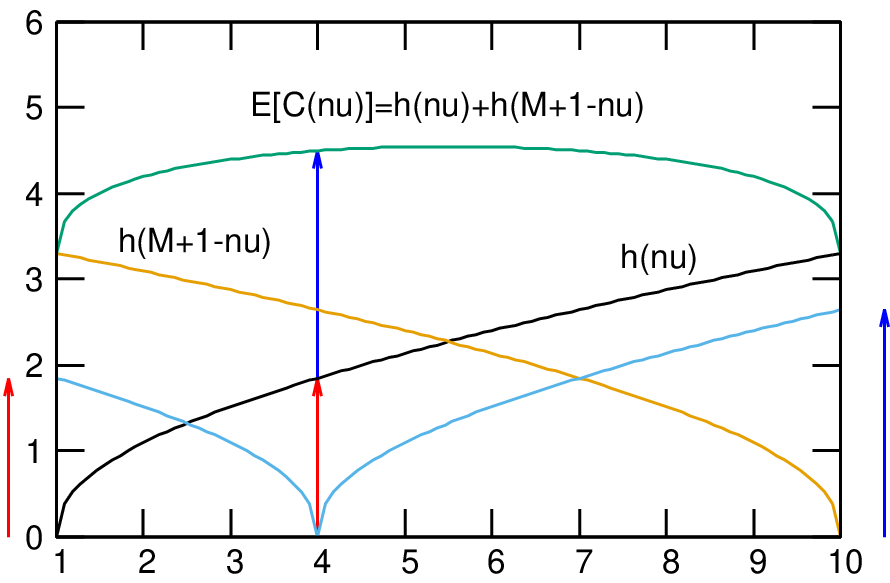
is obtained, and the expectation of makespan can be decomposed into the sum of two terms as follows:

where $\l={\rm E}_{X}[X_{\mu,i}]$. Here we replace $L-t_{M,N}(\nu)=s^{\prime}_{1,1}(M+1-\nu)$ and $L-s_{\nu,1}(\nu)=t^{\prime}_{M+1-\nu,N}(M+1-\nu)$ using an appropriate constant $L$, and ${\rm E}_{X}[t_{M,N}(\nu)-s_{\nu,1}(\nu)]={\rm E}_{X}[t^{\prime}_{M+1-\nu,N}(M+1-\nu)-s^{\prime}_{1,1}(M+1-\nu)]=h(M+1-\nu)$ is obtained by symmetry. The decomposition of ${\rm E}_{X}[C^{\max}(\mu)]$ in Eq.(19) is sketched in Fig. 8.

If $M$ and $N$ are sufficiently large, we can prove some properties of $h(\nu)$, such as concavity, regardless of the probability distribution of $x_{\mu,i}$. Furthermore, an explicit form of function $h(\nu)$ can be obtained for some classes of probability distributions. We will present these results in detail in section 4.

In Fig. 8, an example of the expected terminate time $h(\nu)$ is depicted as a concave function. We can prove that indeed if $M$ and $N$ are sufficiently large, $h(\nu)$ will be a concave function regardless of the probability distribution of $X_{\mu,i}$. However, we will first discuss the relationship between the expectation of makespan and the position of the fiducial machine in the processing system when the processing time is independently and identically distributed according to an exponential distribution. In this discussion, the following representation of the exponential distribution is used:

where $\l$ is the scale parameter and is such that ${\rm E}_{X}[X_{\mu,i}]=\l$ and ${\rm Var}[X_{\mu,i}]={\rm E}_{X}[X^{2}_{\mu,i}]-({\rm E}_{X}[X_{\mu,i}])^{2}=\l^{2}$.

Here we apply $\l=2$ in numerical experiments, the number of machines in this system is $M=1000$, and the number of jobs processed in the processing system is $N=200,400,600$, or $800$. These results for the average of makespan with respect to the index of fiducial machine $\nu$ are shown in Figs. 10 to 12, respectively. The horizontal and vertical axes in these figures indicate the index of the fiducial machine $\nu$ and the average of the makespan ${\rm E}_{X}[C^{\max}(\nu)]$ as evaluated by numerical experiments, respectively. Specifically, the symbols and error bars are results from evaluating $100$ random processing time tables. As shown, the behavior of the mean makespan depends not on the position of the bottleneck machine but on the position of the fiducial machine in this system because the bottleneck machine equivalently exists in the processing system. Moreover using equation (19), the fitting function (solid lines in these figures) is assumed as

where $B=2b+c(M-1)-N{\rm E}_{X}[X_{\nu,i}]$. This equation corresponds to the expected terminate time functions $h(\nu)=A(\nu-1)^{\alpha}+b+c(\nu-1)$ and $h(M+1-\nu)=A(M-\nu)^{\alpha}+b+c(M-\nu)$ already used. These figures show that the results of numerical experiments and fitting functions are consistent with each other. These estimates of parameters are listed in table 3. From this table, it is expected that $\alpha$ is constant with respect to the number of jobs in the case of this exponential distribution; that is, the assumption in equation (19) that the mean of the makespan can be expressed by two expected terminate time functions is satisfied.

Lastly, we compare the above flowshop scheduling results with those using two of the most discussed and applied dispatching rules, shortest processing time (SPT) and longest processing time (LPT). For the case $N=800$ and $M=1000$, the results of applying the two dispatching rules are given in terms of the processing times of machine $1$ in Figs. 14 and 14. As shown, the behaviors of the expectation of makespan for the normal rule scheduling and those of SPT rule scheduling are statistically consistent with each other because the processing time is independently and identically distributed between jobs and machines in the case of large systems, which results in attempts at optimization being canceled out by the randomness of processing time, causing the expected effect of these dispatching rules to be negligible. In fact, $\mathop{\min}_{\nu}({\rm E}_{X}[C^{\max}_{SPT}(\nu)]-{\rm E}_{X}[C^{\max}(\nu)])/{\rm E}_{X}[C^{\max}(\nu)]\simeq-0.0047$ and $\mathop{\max}_{\nu}({\rm E}_{X}[C^{\max}_{SPT}(\nu)]-{\rm E}_{X}[C^{\max}(\nu)])/{\rm E}_{X}[C^{\max}(\nu)]\simeq 0.0012$, where $C^{\max}_{SPT}(\nu)$ and $C^{\max}(\nu)$ are the makespans under the SPT rule and the normal rule, respectively, so that the expected improvement effect is only $0.47\%$, and thus intuitively it is not cost-effective to try to obtain an improvement using the dispatching rule. In contrast, as shown in Figs. 14 and 14, the makespan under LPT scheduling which is not optimal is larger than that under normal scheduling. However, $\mathop{\min}_{\nu}({\rm E}_{X}[C^{\max}_{LPT}(\nu)]-{\rm E}_{X}[C^{\max}(\nu)])/{\rm E}_{X}[C^{\max}(\nu)]\simeq 0.027$ and $\mathop{\max}_{\nu}({\rm E}_{X}[C^{\max}_{LPT}(\nu)]-{\rm E}_{X}[C^{\max}(\nu)])/{\rm E}_{X}[C^{\max}(\nu)]\simeq 0.077$, where $C^{\max}_{LPT}(\nu)$ is the makespan under the LPT rule, so LPT is at most $7.7\%$ worse than normal scheduling.

Next, we also discuss the relationship between the expectation of makespan and the position of the fiducial machine in this system when the processing time is independently and identically distributed according to a discrete uniform distribution, specifically, the following distribution:

which is such that ${\rm E}_{X}[X_{\mu,i}]=7$ and ${\rm Var}[X_{\mu,i}]={\rm E}_{X}[X^{2}_{\mu,i}]-({\rm E}_{X}[X_{\mu,i}])^{2}=14$. As in the previous subsection, the number of machines is $M=1000$ and the number of jobs is $N=200,400,600$, or $800$. The results are shown in Fig. 16 to Fig. 18. As shown, the expectation of makespan under this distribution behaves similarly to the case of an exponential distribution. The estimated parameters in equation (23) for the numerical experiments are listed in table 4.

Next, in order to be able to make a comparison with the previous discrete uniform case, we consider a continuous uniform distribution having the same mean and variance, that is, the density function

is used and is such that ${\rm E}_{X}[X_{\mu,i}]=7$ and ${\rm Var}[X_{\mu,i}]={\rm E}_{X}[X^{2}_{\mu,i}]-({\rm E}_{X}[X_{\mu,i}])^{2}=14$.

Fig. 20 to Fig. 22 show plots of the expectations of makespan for the cases of $N=200,400,600$, and $800$ with $M=1000$. The parameter estimates are listed in table 5. Comparing table 4 and table 5, it is clear that the behaviors of makespan for the two cases are similar up to a statistical fluctuation.

Lastly, the relationship between the average of makespan and the position of the fiducial machine in the processing system is examined for the case that the processing time is independently and identically distributed according to the chi-squared distribution

where ${\rm E}_{X}[X_{\mu,i}]=k$ and ${\rm Var}[X_{\mu,i}]={\rm E}_{X}[X^{2}_{\mu,i}]-({\rm E}_{X}[X_{\mu,i}])^{2}=2k$. If $k=7$, then the mean and variance are consistent with those for the previous uniform distributions. Fig. 24 to Fig. 26 show that the expectation of makespan is concave for this case and similar to the other distributions considered up to a statistical fluctuation. Namely, from these numerical experiments, we can assume that the asymptotical behavior of makespan is universal, that is, it does not depend on the distribution of processing time. The next section will discuss this universality mathematically.

Let discuss the forward scheduling Eq.(5) and Eq.(6). The following argument for forward scheduling can be applied to backward scheduling, by symmetry. Set $T_{0,0}=0$. Then for $(m,n)\in\mathbb{Z}_{\geq 0}^{2}$, we can show

Here, $\{(0,0)\rightsquigarrow(m,n)\}$ means the set of the shortest paths in the square grid graph connecting $(0,0)$ and $(m,n)$. This relation can be derived from Eq.(5) and Eq.(6) by induction.

If $X_{\mu,i}\in\mathbb{R}$ for $\mu,i\in\mathbb{Z}_{\geq 0}$ is sampled i.i.d. from a probability distribution $F$, then the model above is known as the two-dimensional last-passage directed site percolation. This name comes from the problem of finding the time of last-passage of a particle which starts from the origin and moves only in the “right” or “up” direction for a lattice with weights (time required to pass through) on its vertices (rather than its edges). Last-passage directed site percolation has been studied mainly in mathematics and physics [13, 14, 15], and it is also referred to as zero-temperature directed polymer in a random environment when used as a polymer model.

Asymptotic properties of $T_{m,n}$ have been reported (see [15]). Throughout the present paper, we assume ${\rm E}_{X}[X_{\mu,i}]<\infty$ and that $X_{\mu,i}$ is non-degenerate, i.e., ${\rm Var}[X_{\mu,i}]>0$ for any $\mu$ and $i$. There exists a function $g(\vec{v})$ on $\mathbb{R}^{2}_{\geq 0}$ as an almost sure asymptotic limit of $T$: for every $\vec{v}=(v_{1},v_{2})\in\mathbb{R}^{2}_{\geq 0}$,

as $N\rightarrow\infty$. The convergence in $L_{1}$ also holds:

Here, $\displaystyle\mathop{\rightarrow}^{\rm a.s.}$ means almost sure convergence (in other words, convergence with probability one) and $\lfloor\cdot\rfloor$ is the floor function. The function $g(v_{1},v_{2})$ is called a shape function or is sometimes known as a time constant. Note that the existence of such a function $g$ is not obvious but can be proved using Kingman’s subadditive ergodic theorem (see [15]).

Let $\lambda$ be the mean of random variable $X_{\mu,i}$ and $F(X_{\mu,i})$ be its cumulative distribution function. To make the argument simpler, we will use the normalization $\tilde{X}_{\mu,i}=X_{\mu,i}-\lambda$. The corresponding $T_{m,n}$ becomes

Therefore, the corresponding shape function $\tilde{g}$ is represented as

Next we derive makespan for the algorithm in Section 2.5. Assume $M$, the number of machines, and $\nu$, the index of the fiducial machine, are proportional to $N$ in the following sense:

and

for some $\kappa\geq 0$ and $\tau\in[0,1]$. The following theorem states that the normalized makespan is asymptotically represented by the sum of two shape functions.

The proof is in A.

From this theorem, the asymptotic values of the normalized makespan are obtained as

and we can prove the following property of $h_{\kappa}$.

The proof is in B.

For only a few types of distributions $F$ are the shape functions $g$ known. The following theorem is based on the results proved in [14].

References

- [1] Malakooti, B., 2013. Operations and Production Systems with Multiple Objectives. John Wiley & Sons.
- [2] Johnson, S., 1954. Optimal Two- and Three-stage Production Schedules with Setup Times Included, Naval Research Logistics Quarterly, 1(1), pp. 61-68.
- [3] French, S., 1982. Sequencing and Scheduling: An Introduction to the Mathematics of the Job-shop, Horwood, Chichester, UK.
- [4] Garey, M. R., Johnson, D. S., Sethi, R., 1976. The Complexity of Flowshop and Jobshop Scheduling, Mathematics of Operations Research, 1(2), pp. 117-129.
- [5] Nowicki, E., Smutnicki, C. 1996. A Fast Tabu Search Algorithm for the Permutation Flow-shop Problem, European Journal of Operational Research, 91(1), pp. 160-175.
- [6] Osman, I. H., Potts, C. N., 1989. Simulated Annealing for Permutation Flow-shop Scheduling, Omega, 17(6), pp. 551-557.
- [7] Bierwirth, C., Stppler, S., 1992. The Application of a Parallel Genetic Algorithm to the Flowshop Problem, pp.161-175, in New Directions for Operations Research in Manufacturing, edited by Fandel, G., Gulledge T., Jones, A., Springer Verlag.
- [8] Nawaz, M., Enscore, Jr., E. E. and Ham, I., 1983. A Heuristic Algorithm for the -Machine, -Job Flow-shop Sequencing Problem, Omega, 11(1), pp. 91-95.
- [9] Ho, J. C. and Chang, Y.-L., 1991. A New Heuristic for the -Job, -Machine Flow-shop Problem, European Journal of Operational Research, 52(2), pp. 194-202.
- [10] Widmer, M. and Hertz, A., 1989. A New Heuristic Method for the Flow Shop Sequencing Problem, European Journal of Operational Research, 41(2), pp. 186-193.
- [11] Hoos, H. H. and Sttzle, T., 2004. Stochastic Local Search: Foundations and Applications, Morgan Kaufmann.
- [12] Goldratt, E., 1984. The Goal. A Process of Ongoing Improvement. North River Press.
- [13] Corwin, I., 2012. The Kardar-Parisi-Zhang Equation and Universality Class. Random Matrices: Theory and Applications, 1(1), 1130001.
- [14] Johansson, K., 2000. Shape Fluctuations and Random Matrices. Communications in Mathematical Physics. 209(2), pp. 437-476.
- [15] Martin, J. B., 2004. Limiting Shape for Directed Percolation Models. Annals of Probability, 32(4), pp. 2908-2937.
- [16] Rost, H., 1981. Non-equilibrium Behaviour of a Many Particle Process: Density Profile and Local Equilibria. Zeitschrift fur Wahrscheinlichkeitstheorie und Verwandte Gebiete. 58(1), pp. 41-53.