Worst-case Redundancy of Optimal
Binary AIFV Codes and their Extended Codes

In this section, we introduce the definition of a binary AIFV code proposed in [5]. A binary AIFV code uses two binary code trees, denoted by $T_{0}$ and $T_{1}$, in such a way that the code is uniquely decodable and the decoding delay is at most two bits. As conventional FV codes, a source symbol is assigned to a node of the code trees and a code symbol is assigned to an edge of the trees. We begin with a list of properties satisfied by the trees of a binary AIFV code.

1. 1.

   Incomplete internal nodes (nodes with one child) are divided into two categories, master nodes and slave nodes.

2. 2.

   Source symbols are assigned to either master nodes or leaves.

3. 3.

   The child of a master node must be a slave node, and the master node is connected to its grandchild by code symbols ‘00’.

4. 4.

   The root of $T_{1}$ has two children. The child connected by ‘0’ from the root is a slave node. The slave node is connected by ‘1’ to its child.

Fig. 1 illustrates an example of a binary AIFV code for $\mathcal{X}=\{a,b,c,d\}$, where slave nodes are marked with squares. It is easy to see that the trees satisfy all the properties of a binary AIFV code.

Given a source sequence $x_{1}x_{2}x_{3}\cdots$, an encoding procedure of a binary AIFV code goes as follows.

Using a binary AIFV code of Fig. 1, a source sequence ‘$acdbaca$’ is encoded to ‘0.11.1100.10.0.11.01’, where dots ‘.’ are inserted for the sake of human readability, but they are not necessary in the actual codeword sequences. The code trees are visited in the order of $T_{0}\rightarrow T_{0}\rightarrow T_{1}\rightarrow T_{0}\rightarrow T_{0}\rightarrow T_{0}\rightarrow T_{1}$.

A codeword sequence $y_{1}y_{2}y_{3}\cdots\in\{0,1\}^{*}$ is decoded as follows.

The decoding procedure is guaranteed to visit the code trees in the same order as the corresponding encoding process does [5]. The codeword sequence ‘01111001001101’ is indeed decoded to the original source sequence ‘$acdbaca$’, using a sequence of trees in the order of $T_{0}\rightarrow T_{0}\rightarrow T_{1}\rightarrow T_{0}\rightarrow T_{0}\rightarrow T_{0}\rightarrow T_{1}$. When all source symbols are assigned to leaves of $T_{0}$, a binary AIFV code reduces to an instantaneous FV code.

The following defines the average code length of a binary AIFV code, denoted by $L_{\rm AIFV}$.

where $P(T_{0})$ (resp. $P(T_{1})$) is a stationary probability of $T_{0}$ (resp. $T_{1}$), and $L_{T_{0}}$ (resp. $L_{T_{1}}$) is the average code length of $T_{0}$ (resp. $T_{1}$). Consider for instance, a source $\mathcal{X}=\{a,b,c,d\}$ with probabilities $P(a)=0.45,\ P(b)=0.3,\ P(c)=0.2,\ P(d)=0.05$. Fig. 1 depicts an example of binary AIFV code trees for this source. It follows from the encoding procedure 1 that the transition probabilities $P(T_{1}|T_{0})$ and $P(T_{0}|T_{1})$ are given by $0.2$ and $0.8$, respectively. Therefore, the stationary probabilities $P(T_{0})$ and $P(T_{1})$ are calculated as 0.8 and 0.2, respectively. Thus, we get $L_{{\rm AIFV}}=1.65\cdot 0.8+2.1\cdot 0.2=1.74$. On the other hand, it is easy to see that the average code length of the corresponding Huffman code is 1.8. In this example, we see that the binary AIFV code outperforms the Huffman code in terms of compression ratio.

It is worth noting that the root of $T_{0}$ is allowed to be a master node, to which a source symbol is assigned. Fig. 2 illustrates an example of a binary AIFV code for $\mathcal{X}=\{a,b,c\}$, where $a$ is assigned to the root of $T_{0}$. The code trees again satisfy all the properties of a binary AIFV code. Using the binary AIFV code of Fig. 2, a source sequence ‘$aabac$’ is encoded to ‘$\lambda$.1.000.$\lambda$.011’, where $\lambda$ is the null codeword corresponding to the root of $T_{0}.$ The code trees are visited in the order of $T_{0}\rightarrow T_{1}\rightarrow T_{0}\rightarrow T_{0}\rightarrow T_{1}$. We see that in binary AIFV codes, source symbols are sometimes encoded with $\lambda$, i.e., via pure tree transitions without outputting any code symbol. It is easy to confirm that the codeword sequence ‘1000011’ is decoded to the original source sequence and decoding procedure visits the code trees in the same order as the encoding procedure does. Note that since the first codeword ‘1’ on the code sequence cannot be traced on $T_{0}$ of Fig. 2, we output ‘$a$’, which is assigned to the root of $T_{0}$.

Lastly, we define the redundancy of optimal binary AIFV codes. Let $L_{{\rm OPT}}$ be the average code length of the optimal binary AIFV code for a given source. Then the redundancy of optimal binary AIFV codes denoted by $r_{{\rm AIFV}}$ is defined as

where $X$ is a random variable corresponding to the source and $H(X)$ is the source entropy. It is shown in [5] how we can obtain the optimal binary AIFV code trees for a given source.

Sibling property was first introduced in [6] as a structural characterization of Huffman codes. Consider a $K$-ary source and let $T_{\rm H}$ denote the corresponding Huffman tree. Let the weight of a leaf be the probability of corresponding source symbol. Also, let the weight of an internal node be defined recursively as the sum of the weights of the children. There are $2K-2$ nodes (except the root) on $T_{\rm H}$. Let $q_{1},q_{2},\dots,q_{2K-2}$ be the weights of the nodes sorted in a non-increasing order, so that $q_{1}\geq q_{2}\geq\cdots\geq q_{2K-2}$. By a slight abuse of notation, we identify $q_{k}$ with the corresponding node itself in the rest of the paper.

We state the sibling property of Huffman codes, which will play an important role in the later proofs of the redundancy of optimal binary AIFV codes.

It is well-known that the worst-case redundancy of Huffman codes is 1. Meanwhile, numerous studies have shown that better bounds on the redundancy can be obtained when a source satisfies some predefined conditions. One such condition concerns with the value of $p_{\max}$ [6]–[10], where $p_{\max}$ is the probability of the most likely source symbol. The following is proved by Gallager [6].

In Fig. 3, we summarize the upper bound results for Huffman codes in terms of $p_{\max}$ [11]. For $p_{\max}\geq\frac{1}{6}$, the bound is shown to coincide with the worst-case redundancy of the codes in terms of $p_{\rm max}$. We see from Fig. 3 that the redundancy upper bound of Huffman codes approaches to its worst-case redundancy, 1, only when source probabilities are extremely biased.

We start with redefining a ‘slave node’ and a ‘master node’ that were defined in Section II-A.

In the later figures, slave nodes are marked by square nodes. To distinguish two kinds of slave nodes, a slave-1 (resp. slave-0) node is marked by a white (resp. black) square node.

In contrast to the previous definition of master nodes provided in Section II-A, we note that the new definition of master nodes includes leaves. Fig. 4 illustrates a master node of degree $k\geq 1$. The master node in Section II-A corresponds to a master node of degree 1 in Definition 3.

Let $m$ be a natural number. As an extension of the original binary AIFV code, we define a binary AIFV-$m$ code, which uses $m$ code trees and decoding delay is at most $m$ bits. The code trees $T_{0},\ T_{1},\ \dots,T_{m-1}$ of a binary AIFV-$m$ code are defined by the following properties.

1. 1.

   Any node in the code trees is either a slave node, a master node, or a complete internal node. Conforming to Definitions 2 and 3, source symbols are only assigned to master nodes.

2. 2.

   The degree $k$ of master nodes must satisfy $0\leq k\leq m-1.$

3. 3.

   $T_{i},\ 1\leq i\leq m-1$, has a node connected to the root by $\underbrace{00\cdots 0}_{i}$ and it is a slave-1 node.

We proceed to explain encoding and decoding procedures of the binary AIFV-$m$ codes. Given a source sequence $x_{1}x_{2}x_{3}\cdots$, the encoding procedure is described as follows.

A codeword sequence $y_{1}y_{2}y_{3}\cdots\in\{0,1\}^{*}$ is decoded as follows.

In this procedure, the source symbol at a master node of degree $k\geq 1$ is decoded after reading subsequent $k+1$ code symbols. Thus, the decoding delay of binary AIFV-$m$ codes is at most $m$ bits.

In the following, we show two examples of binary AIFV-$m$ codes to demonstrate how the codes work.

The root of $T_{i},\ i\neq 1$, can also be a master node. Example 2 shows this case.

We show a lemma, which is crucial to prove the unique decodability of binary AIFV-$m$ codes in Theorem 3.

We prove by induction that for all $2\leq\ell\leq m$, when the encoding procedure starts from the root of $T_{i},~1\leq i\leq\ell-1$, the code sequence does not start with $\underbrace{00\cdots 0}_{i+1}$.

The base case $(\ell=2)$ holds since the root of $T_{1}$ cannot be a master node and any codewords of $T_{1}$ do not have prefix ‘00’.

Suppose that the induction hypothesis holds for some $\ell$ such that $2\leq\ell\leq m-1$. Our goal is to show that the induction hypothesis also holds for $\ell+1$. To this end, it is sufficient to show that when the encoding procedure starts from the root of $T_{\ell}$, the code sequence does not start with $\underbrace{00\cdots 0}_{\ell+1}$. We consider the following two cases.

1. 1.

   The first symbol in the source sequence is not assigned to a node connected by a sequence of 0’s from the root of $T_{\ell}$.

2. 2.

   The first symbol in the source sequence is assigned to a master node (which we denote as $M$) connected by $\underbrace{00\cdots 0}_{j}$, $0\leq j\leq\ell-2$, from the root of $T_{\ell}$.

To begin with, consider the first case. It follows from property 3) of binary AIFV-$m$ code trees that any codewords of $T_{\ell}$ do not have prefix $\underbrace{00\cdots 0}_{\ell+1}$. Hence, the encoding procedure would not output a codeword sequence that starts with $\underbrace{00\cdots 0}_{\ell+1}$.

We then consider the second case. It follows from Definition 3 that the degree of $M$ (which we denote as $k$) must satisfy $1\leq k\leq\ell-j-1$. When the source symbol assigned to $M$ in $T_{\ell}$ is encoded, the encoding procedure would output codeword $\underbrace{00\cdots 0}_{j}$ and then use $T_{k}$ for the next code tree. By the induction hypothesis, when the encoding procedure starts from the root of $T_{k}$, the codeword sequence does not start with $\underbrace{00\cdots 0}_{k+1}$. Therefore, the concatenated codeword sequence does not start with $\underbrace{00\cdots 0}_{j}\underbrace{00\cdots 0}_{k+1}$, which implies that the sequence does not start with $\underbrace{00\cdots 0}_{\ell}$.

In both cases, when the encoding procedure starts from the root of $T_{\ell}$, the code sequence does not start with $\underbrace{00\cdots 0}_{\ell+1}$. $\Box$

Let $x_{1}x_{2}x_{3}\cdots$ be a source sequence and let $x^{\prime}_{1}x^{\prime}_{2}x^{\prime}_{3}\cdots$ be the recovered source sequence. Also, let $i_{p}$ (resp. $j_{p}$) be a position on codeword sequence $(y_{1}y_{2}y_{3}\cdots)$ from which encoding (resp. decoding) of $x_{p}$ starts, and let $T^{p}_{{\rm enc}}$ (resp. $T^{p}_{{\rm dec}}$) be a code tree used to encode (resp. decode) $x_{p}.$ We prove by induction that $i_{p}=j_{p}$ and $T^{p}_{{\rm enc}}=T^{p}_{{\rm dec}}$ hold for every $p\geq 1.$

The base case $(p=1)$ clearly holds since $i_{1}=j_{1}=1$ and $T^{1}_{{\rm enc}}=T^{1}_{{\rm dec}}=T_{0}$.

Suppose that $i_{p}=j_{p}$ and $T^{p}_{{\rm enc}}=T^{p}_{{\rm dec}}$ hold for a given $p\geq 1$. Our goal is to prove $i_{p+1}=j_{p+1}$ and $T^{p+1}_{{\rm enc}}=T^{p+1}_{{\rm dec}}$. We note that $x_{p}$ is assigned to a master node. First, suppose that $x_{p}$ is assigned to a master node of degree 0, i.e., a leaf. Then, the decoding procedure straightforwardly recovers $x_{p}$ with no decoding delay. Thus, $x^{\prime}_{p}=x_{p}$ holds and so does $i_{p+1}=j_{p+1}$. Then, both the encoder and decoder visit $T_{0}$ for the next source symbol $x_{p+1}$. Hence, $T^{p+1}_{{\rm enc}}=T^{p+1}_{{\rm dec}}$ holds. Next, suppose that $x_{p}$ is assigned to a master node of degree $k\geq 1$ (which we denote as $M$). Then, the encoding procedure visits $T_{k}$ for the next symbol $x_{p+1}$. We note from Lemma 1 that the code sequence does not start with $\underbrace{00\cdots 0}_{k+1}$, when the encoding procedure starts from the root of $T_{k}$. On the other hand, since $M$ is a master node of degree $k$, we see from Definition 3 that the prefix of all codeword sequences on $T_{{\rm enc}}^{p}$ starting from $M$ is $\underbrace{00\cdots 0}_{k+1}$. Thus, the decoding procedure cannot trace any codeword starting from $M$. Therefore, the decoding procedure decodes a source symbol at $M$, which leads the decoder to use $T_{k}$ for the next source symbol $x_{p+1}$. Hence, $x_{p}=x^{\prime}_{p},\ i_{p+1}=j_{p+1}$ and $T^{p+1}_{{\rm enc}}=T^{p+1}_{{\rm dec}}$ hold. In either cases, $i_{p+1}=j_{p+1}$ and $T^{p+1}_{{\rm enc}}=T^{p+1}_{{\rm dec}}$ hold.

From the above induction, we have that $i_{p}=j_{p}$ and $T^{p}_{{\rm enc}}=T^{p}_{{\rm dec}}$ and hence $x_{p}$ = $x^{\prime}_{p}$, which means that binary AIFV-$m$ codes are uniquely decodable. $\Box$

We proceed to define an average code length $L_{{\rm AIFV}}$ and redundancy $r_{{\rm AIFV}}$ of binary AIFV-$m$ code.

Redundancy of optimal binary AIFV-$m$ codes is defined in the same way as (2).

Based on Definition 4, we show how to calculate the average code length of binary AIFV-$m$ code. For example, consider the code trees in Fig. 5 for a source $\mathcal{X}=\{a,b,c,d\}$ with probabilities $P(a)=0.65,\ P(b)=0.2,\ P(c)=0.1$ and $P(d)=0.05.$ The transition matrix $R$ is given by

where $R_{ij}$ denotes the transition probability $P(T_{j}|T_{i})$ from $T_{i}$ to $T_{j}$. The vector $\mbox{\boldmath$p$}=(P(T_{0}),P(T_{1}),\dots,P(T_{m-1}))^{\top}$ of stationary probabilities satisfies

Therefore, $p$ is the normalized left eigenvector of $R$ with eigenvalue of 1. Hence, we get $P(T_{0})=\frac{100}{111},\ P(T_{1})=\frac{10}{111}$ and $P(T_{2})=\frac{1}{111}.$ By Definition 4, the average code length $L_{{\rm AIFV}}$ is calculated as

We proceed to show the calculation of the average code length of the code in Fig. 6 for a source with probabilities $P(a)=0.98,\ P(b)=0.01,$ and $P(c)=0.01$. The transition matrix $R$ is obtained as

Hence, we get the stationary probabilities as $P(T_{0})=\frac{2500}{7351}\approx 0.340,\ P(T_{1})=\frac{2401}{7351}\approx 0.327,$ and $P(T_{2})=\frac{2450}{7351}\approx 0.333$. From (3), the average code length $L_{{\rm AIFV}}$ is calculated as

Note that average code lengths of $T_{0}$ and $T_{2}$ are much smaller than 1. This is because the most likely source symbol ‘$a$’ is assigned to the roots of the trees. Compared with Fig. 2, which uses only two code trees, the binary AIFV-3 code shown in Fig. 6 uses an additional code tree $T_{2}$. The introduction of $T_{2}$ enables the extended code to compress the source better than the original binary AIFV code in Fig. 2.

Fig. 7 compares the worst-case redundancy given by Theorems 2 and 4. We see that the worst-case redundancy of optimal binary AIFV codes is smaller than that of Huffman codes for every $p_{\max}\geq\frac{1}{2}$.

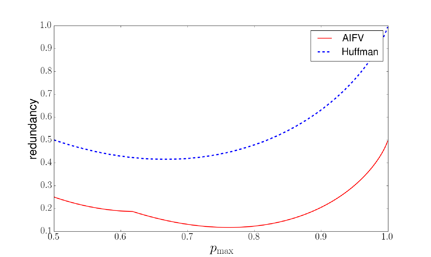
We also get Theorem 5, covering the case of $p_{\max}<\frac{1}{2}$.

The bound given by Theorem 5 may not be tight for each $p_{\rm max}\in\left(0,\frac{1}{2}\right)$ and does not necessarily coincide with the worst-case redundancy of optimal binary AIFV codes for sources with $p_{\rm max}\in\left(0,\frac{1}{2}\right)$. Yet, the derived bound is sufficient to prove Corollary 1, which follows immediately from Theorems 4 and 5.

Note that the worst-case redundancy given in Corollary 1 is the same as that of Huffman codes constructed for $\mathcal{X}^{2}$. It is also empirically shown that for some sources, optimal binary AIFV codes can beat Huffman codes for $\mathcal{X}^{2}$ [5]. Meanwhile, in terms of memory efficiency, a binary AIFV code only requires $\mathcal{O}(K)$ for storing code trees, while a Huffman code for $\mathcal{X}^{2}$ needs $\mathcal{O}(K^{2})$, where $K=|\mathcal{X}|$. These suggest that binary AIFV codes are more memory-efficient than Huffman codes for $\mathcal{X}^{2}$, while attaining comparable compression performance both empirically and theoretically.

Do binary AIFV-$m$ codes provide further compression improvement over the original binary AIFV codes? In the following, we obtain the worst-case redundancy of optimal binary AIFV-$m$ codes for $m=3$ and 4. These results suggest that binary AIFV-$m$ codes can benefit from the use of more code trees.

Although the above theorems provide the worst-case redundancy of optimal binary AIFV-$m$ codes for the case of $m=3$ and 4, we conjecture that for any natural number $m$, the worst-case redundancy of optimal AIFV-$m$ codes is also $\frac{1}{m}$. Our justification for the conjecture is as follows. Huffman codes and the optimal AIFV-$m$ codes for $m\leq 4$ have the worst-case redundancy when $p_{\max}\to 1$. Thus, it is natural to assume that the same property also holds for $m\geq 5$. If this assumption is true, then the worst-case redundancy is $\frac{1}{m}$ from Theorem 9, although it is an open question whether this assumption holds or not.

References

- [1] L. G. Kraft, “A device for quanitizing, grouping and coding amplitude modulated pulses,” Master thesis, Department of Electrical Engineering, MIT, 1949.
- [2] B. McMillan, “Two inequalities implied by unique decipherability,” Inform. Theory, IRE Trans., vol. IT-2, no. 4, pp. 115–116, 1956.
- [3] D. A. Huffman, “A method for the construction of minimum redundancy codes,” Proceedings of the IRE, vol. 40, no. 9, pp. 1098–1101, 1952.
- [4] H. Yamamoto and X. Wei, “Almost instantaneous FV codes,” in Proceedings of the 2013 IEEE ISIT, Istanbul, Turkey, 2013, pp. 1759–1763.
- [5] H. Yamamoto, M. Tsuchihashi, and J. Honda, “Almost instantaneous fixed-to-variable length codes,” IEEE Trans. Inform. Theory, vol. 61, no. 12, pp. 6432–6443, 2015.
- [6] R. G. Gallager, “Variations on a theme by Huffman,” IEEE Trans. Inform. Theory, vol. IT-24, no. 6, pp. 668–674, 1978.
- [7] B. L. Montgomery and J. Abrahams, “On the redundancy of optimal binary prefix-condition codes for finite and infinite sources,” IEEE Trans. Inform. Theory, vol. 33, no. 1, pp. 156–160, 1987.
- [8] D. Manstetten, “Tight bounds on the redundancy of Huffman codes,” IEEE Trans. Inform. Theory, vol. 38, no. 1, pp. 144–151, 1992.
- [9] R. M. Capocelli and A. D. Santis, “Tight upper bounds on the redundancy of Huffman codes,” IEEE Trans. Inform. Theory, vol. 35, no. 5, pp. 1084–1091, 1989.
- [10] O. Johnsen, “On the redundancy of binary Huffman codes,” IEEE Trans. Inform. Theory, vol. IT-26, no. 2, pp. 220–222, 1980.
- [11] C. Ye and R. W. Yeung, “A simple upper bound on the redundancy of Huffman codes,” IEEE Trans. Inform. Theory, vol. 48, no. 7, pp. 2132–2138, 2002.
- [12] W. Szpankowski, “Asymptotic average redundancy of Huffman (and other) block codes,” IEEE Trans. Inform. Theory, vol. 46, no. 7, pp. 2434–2443, 2000.