A one-particle quantum system in a pure state is described by a unit vector in some Hilbert space (or to be precise, by the projection onto the corresponding line). For multi-particle systems, the associated Hilbert space is simply given by the tensor product of the individual ones. Its dimension thus grows exponentially with the number of subsystems, making the classical modelling of quantum systems practically unfeasible as soon as more than a few particles are involved.

One way around this curse of dimensionality is to make use of any extra information which may be held, a priori, on the state of the system under consideration. One could know, for instance, that the latter has certain symmetries, and exploit the reduction in the effective number of degrees of freedom that this fact implies. The archetypical example is the following: Assume that a system is composed of $n$ indistinguishable particles (meaning that their labelling is irrelevant), with associated finite-dimensional Hilbert space $\mathrm{H}$. Then, a pure state of such system actually lives in the symmetric subspace $\mathrm{Sym}^{n}(\mathrm{H})$ of $\mathrm{H}^{\otimes n}$, whose dimension is only polynomial, rather than exponential, in $n$.

On the other hand, one should not conclude too quickly that having to deal with high dimensional objects is necessarily a misfortune. Indeed, it may also be the case that, as the dimension grows, certain universal behaviours emerge. This is precisely what asymptotic geometric analysis and random matrix theory teach us. In quantum information theory, these subfields of mathematics can serve at least two main purposes. First of all, they may be used as a tool to determine what are the properties that big quantum systems, subject to whatever relevant restrictions, are expected to exhibit. More concretely, one could be interested in knowing what are the typical characteristics of either quantum states or quantum transformations, under several types of constraints such as locality, noise, energy etc. Second of all, they may help in proving the existence of objects having a given property. In this context, the paradigmatic idea is that constructing the latter explicitly might be harder than asserting that a suitably chosen random one will do with overwhelming probability. And with both aims in view, high dimension of the underlying space is an asset, what makes average features become generic.

The purpose of this thesis is therefore clearly two-sided: in some places the focus is on how to reduce the study of large (or even infinite) dimensional situations to that of lower dimensional ones, while in some others the goal is precisely to understand the typical aspects which may arise as the dimension of the studied object grows. The latter objective is clearly the underlying motivation of Part III. As for the former objective, two different routes can be taken to achieve it. The first approach, which is the one followed in Part II, consists in trying to compress the initial data set as much as possible while still preserving the essential information it contains. The second approach consists in exploiting potential additional knowledge on the initial data to argue that they already belong, effectively, to a much smaller set. This is the spirit of Part IV.

All the questions posed here initially arise from quantum information theory. But in order to solve them, several fields of pure mathematics had to get heavily involved. For a start, random matrix theory plays undeniably a prominent role in all our work. Nevertheless, we are not so much preoccupied with the asymptotic study of random matrices, as (free) probabilists usually are, but rather with the non-asymptotic one. Indeed, for the applications we have in mind, knowing that a certain behaviour emerges almost surely in the regime where the size of the matrix goes to infinity is not so useful: we need instead to understand, for a large but finite size, what is the probability that the properties of the matrix do not deviate too much from their limiting ones. This is where concentration of measure enters the picture, allowing us to assert that, if the function we are looking at is regular enough, then it should be close to its expected value with overwhelming probability as the size of its random input grows. We exploit this key phenomenon under multiple forms throughout these pages. It however appears clear that, before even trying to bound the deviation probability of a given function (and more often than not, also as an end in itself), we have to be able to estimate its average value. For that purpose, we usually call in geometric and probabilistic techniques in Banach space theory. Besides, taking advantage of the symmetries of our problem, is an idea that we try to apply whenever possible. With that goal in view, information theory tools, both classical and quantum, are crucial to us. They are in fact what makes it for instance possible to relate in a quantitative way exchangeability and independence.

Each chapter revolves around a piece of work which either already led to a paper (sometimes published yet, sometimes in preprint form still) or should lead to one shortly. In each case though, modifications have been done on the original version. Occasionally it is just a matter of notation or presentation, to simply fit better with the rest of the manuscript (unfortunately, it is likely that neither complete non-redundancy nor absolute style unity have been achieved between the chapters). But here and there further developments, that were investigated only afterwards, have also been added.

The remainder of this introductory part is dedicated to setting the common ground and tools on which subsequent parts develop. If it achieves the goal it was designed for, Chapter 2 could be renamed “Everything you need to know about quantum physics if you are a mathematician willing to read this manuscript”. As for Chapters 3 and 4, they can be seen as the two toolboxes in which we will regularly dig: in Chapter 3 for all the basics about permutation-symmetry, and in Chapter 4 for all the basics about high dimensional convex geometry and deviation inequalities.

As already mentioned, the core scientific material in this thesis is then divided into three parts. Let us try to summarize in a few words the content of each of them, even though the needed definitions in order to do so in a satisfactory way have not been introduced yet (see Chapter 2 for most of them). Precisely for that matter, it is only at the beginning of each part that a proper account is made of its objectives, its main achievements (and techniques to reach them), its non-ignorable difficulties etc.

The main theme of Part II is that of approximating complex processes by simpler ones. In Chapter 5 the question which is investigated is: given a quantum channel, to how much can its number of Kraus operators be brought down, with the constraint that each input state is still sent close to its original output state? In some sense, Chapter 6 deals with a similar issue. Nevertheless, the channels which are now considered are quantum-classical channels (aka quantum measurements), and the approximation requirement is completely different: namely that, for each input state, outcome statistics close to its original ones are obtained. Our objective in both cases is to exhibit universal schemes which attain the maximum doable compression.

The goal of Part III is to study several properties of quantum states (more specifically, entanglement-related properties of multipartite quantum states), and see how (un)common they become as the size of the quantum system grows. Chapter 7 is in line with Chapter 6 since it also focusses on the issue of distinguishing quantum states from their measurement outcome statistics. But this time the question is: how well can local observers, having access only to their own subsystem, typically perform in this task? Then, in both Chapters 8 and 9, the aim is to quantify the average strength of certain semidefinite relaxations of separability. In Chapter 8, stress is put on exporting entanglement detection tools from the bipartite setting, relying on positive maps, to certify genuinely multipartite entanglement. Oppositely, the interest in Chapter 9 is in a purely bipartite and not positive map based separability criterion (more precisely, a complete hierarchy of necessary conditions for bi-separability build on symmetric extensions).

This opens naturally the route to Part IV, where symmetries are exploited to their maximum, with the purpose of reducing the understanding of permutation-invariant scenarios to that of i.i.d. ones. Hence, a major difference with Part II is that we are now making extensive use of the specificities of the situation we have at hand in order to get a highly problem-dependent simplification. Chapter 10 is dedicated to setting a very general and adaptable framework in which one can indeed do so. As a consequence, several quantities arising in quantum information theory can be shown to exhibit a multiplicative behaviour. Chapter 11 is then entirely devoted to seeing through one important application of the previously developed machinery, namely to the parallel repetition problem for multi-player non-local games.

Perhaps now is the time to fleetingly elaborate on the choice of the thesis title. There are two distinct ways in which we are principally dealing with “high dimension”: either because we are looking at one system whose underlying dimension is large, or because we are looking at many copies of a system. Yet, in both situations “symmetries” play a central role. To attack the first problem, it is usually tools from asymptotic geometric analysis that we call on for help. This field of mathematics can be seen as a middle ground between geometry (which traditionally deals with small-dimensional objects) and functional analysis (which traditionally deals with infinite-dimensional objects). And its whole purpose is to identify and exploit approximate symmetries that escaped both the too rigid area of geometry and the too qualitative area of functional analysis. As for the second issue, it is usually tackled via information theory techniques. And it is more often than not making use of the permutation-symmetry of the multi-copy scenario which allows relating asymptotic performances to single-shot ones, and hence get an understanding of them.

This manuscript essentially puts together the material appearing in the following publications or preprints:

• •

  C. Lancien. Quantum channel compression.
  In preparation. (cf. Chapter 5)
  

• •

  G. Aubrun and C. Lancien. Zonoids and sparsification of quantum measurements.
  Positivity, 20(1):1–23, 2016. arXiv[quant-ph]:1309.6003 (cf. Chapter 6)
  

• •

  G. Aubrun and C. Lancien. Locally restricted measurements on a multipartite quantum system: data hiding is generic.
  Quant. Inf. Comput., 15(5–6):512–540, 2014. arXiv[quant-ph]:1406.1959. (cf. Chapter 7)
  

• •

  O. Gühne, M. Huber, C. Lancien and R. Sengupta. Relaxations of separability in multipartite systems: semidefinite programs, witnesses and volumes.
  J. Phys. A: Math. Theor., 48(505302), 2015. arXiv[quant-ph]:1504.01029. (cf. Chapter 8)
  

• •

  C. Lancien. k-extendibility of high-dimensional bipartite quantum states.
  Preprint. arXiv[quant-ph]:1504.06459. (cf. Chapter 9)
  

• •

  C. Lancien and A. Winter. Flexible constrained de Finetti reductions and applications.
  Preprint. arXiv[quant-ph]:1605.09013. (cf. Chapter 10)
  

• •

  C. Lancien and A. Winter. Parallel repetition and concentration for (sub-)no-signalling games via a flexible constrained de Finetti reduction.
  Preprint. arXiv[quant-ph]:1506.07002. (cf. Chapter 11)
  

Other publications or preprints on which this manuscript does not focus:

• •

  C. Lancien and A. Winter. Distinguishing multi-partite states by local measurements.
  Commun. Math. Phys., 323:555–573, 2013. arXiv[quant-ph]:1206.2884.
  

• •

  G. Adesso, S. Di Martino, M. Huber, C. Lancien, M. Piani and A. Winter. Should entanglement measures be monogamous or faithful?
  Preprint. arXiv[quant-ph]:1604.02189.
  

Here is a list of notation that shall be used repeatedly throughout the whole manuscript (it might happen though that some are recalled as the text goes). Oppositely, notation which are needed more sporadically will be introduced only in due time.

Given a complex Hilbert space $\mathrm{H}$, we denote by $\mathcal{L}(\mathrm{H})$ the space of all linear operators on $\mathrm{H}$. When $\mathrm{H}\equiv\mathbf{C}^{d}$ is finite-dimensional (which will almost always be the case we will be dealing with), we identify $\mathcal{L}(\mathrm{H})$ with the space of $d\times d$ complex matrices. Important subsets of $\mathcal{L}(\mathrm{H})$ include: the group of unitary operators on $\mathrm{H}$, which we denote by $\mathcal{U}(\mathrm{H})$, the space of Hermitian operators on $\mathrm{H}$, which we denote by $\mathcal{H}(\mathrm{H})$, the cone of positive semidefinite operators on $\mathrm{H}$, which we denote by $\mathcal{H}_{+}(\mathrm{H})$. The notation $\mathrm{Id}$ (or $\mathrm{Id}_{\mathrm{H}}$ if there is a risk of confusion) stands for the identity operator on $\mathrm{H}$, while the notation $\mathcal{I\!d}$ (or $\mathcal{I\!d}_{\mathrm{H}}$) is used for the identity (super-)operator on $\mathcal{L}(\mathrm{H})$. Also, for any $X\in\mathcal{L}(\mathrm{H})$, we denote by $X^{\dagger}$ its adjoint (i.e. transpose conjugate) and by $|X|=\sqrt{X^{\dagger}X}$ its absolute value.

For each $p\in[1,+\infty]$, we define $\|\cdot\|_{p}$ as the Schatten $p$-norm on $\mathcal{L}(\mathrm{H})$, i.e.

Particular instances of interest are the trace class norm $\|\cdot\|_{1}$, the Hilbert–Schmidt norm $\|\cdot\|_{2}$ (which is nothing else than the Euclidean norm arising from the Hilbert–Schmidt inner product $\langle X,Y\rangle\mapsto\tr\left(X^{\dagger}Y\right)$ on $\mathcal{L}(\mathrm{H})$), and the operator norm $\|\cdot\|_{\infty}$. Most of the time, we will look at Schatten $p$-norms not on the full space $\mathcal{L}(\mathrm{H})$ but in restriction to its subspace $\mathcal{H}(\mathrm{H})$. We denote by $B_{p}(\mathrm{H})$, resp. $S_{p}(\mathrm{H})$, the corresponding unit ball, resp.  sphere, in $\mathcal{H}(\mathrm{H})$. In the special case $p=2$, we may also use the notation $B_{HS}(\mathrm{H})$ and $S_{HS}(\mathrm{H})$ instead.

We denote by $\|\cdot\|_{p}$ as well the $p$-norms on $\mathbf{R}^{d}$ or $\mathbf{C}^{d}$. One exception is again the Euclidean norm $\|\cdot\|_{2}$, for which we shall usually simply use the notation $\|\cdot\|$, while $S^{d-1}$ and $S_{\mathbf{C}^{d}}$ stand for the corresponding Euclidean unit spheres in $\mathbf{R}^{d}$ and $\mathbf{C}^{d}$, respectively.

The notation $|\cdot|$ stands both for the cardinality when applied to a finite set and for the dimension when applied to a finite-dimensional Hilbert space.

Given $n\in\mathbf{N}$, we may use the shorthand notation $[n]$ for $\{1,\ldots,n\}$, and we denote by $\mathfrak{S}(n)$, resp. $\mathfrak{P}(n)$, the set of permutations, resp. partitions, of $[n]$.

In the remainder of this manuscript, we are often interested in the asymptotic regime, when the dimensions of the underlying finite-dimensional Hilbert spaces tend to infinity. In that setting, the letters $C,c,c_{0},\ldots$ will always denote (non-negative) numerical constants, independent from any other parameters such as the dimension. The value of these constants may change from occurrence to occurrence. Similarly $c(\varepsilon)$ denotes a constant depending only on the parameter $\varepsilon$. Also, given functions $f,g$ of the underlying dimension $d$, we will write $f=O(g)$, resp. $f=\Omega(g)$, if there exists $C>0$ such that, for all $d\in\mathbf{N}$, $f(d)\leqslant Cg(d)$, resp. $f(d)\geqslant g(d)/C$, and we will write $f=\Theta(g)$ if both $f=O(g)$ and $f=\Omega(g)$ hold.

When working with a random variable $X$, we will use the notation $\mathbf{P}(\mathcal{E}(X))$ to denote the probability of the event $\mathcal{E}(X)$, and the notation $\E\left(f(X)\right)$ to denote the expectation of the function $f(X)$.

More quantum information orientated notation include (see Chapter 2, Sections 2.1 and 2.2, for the corresponding definitions): $\mathcal{D}(\mathrm{H})$ for the set of quantum states on the Hilbert space $\mathrm{H}$, $\mathcal{S}(\mathrm{H}_{1}{:}\cdots{:}\mathrm{H}_{k})$ for the set of separable quantum states on the tensor product Hilbert space $\mathrm{H}_{1}\otimes\cdots\otimes\mathrm{H}_{k}$ (across the $k$-partite cut $\mathrm{H}_{1}{:}\cdots{:}\mathrm{H}_{k}$).

In quantum mechanics, the state of a system is described by a unit vector $\psi$ in a complex separable Hilbert space $(\mathrm{H},\langle\cdot|\cdot\rangle)$. The physical picture is then the following: There exists a distinguished orthonormal basis $\{e_{i},\ i\in I\}$ of $\mathrm{H}$, where $I$ is countable (finite or infinite) and labels the possible “levels” of the system. If $\psi=e_{i}$ for some $i\in I$, then (as one would expect) the system is said to be in level $i$. But in general, $\psi$ is in a superposition of the basis vectors, i.e.

And the only thing that one can tell is that the probability of obtaining outcome $i\in I$ when measuring its level is given by $|\langle e_{i}|\psi\rangle|^{2}$. We already see with this description that, for any $\alpha\in\mathbf{C}$ such that $|\alpha|^{2}=1$, states $\psi$ and $\alpha\psi$ cannot be distinguished. It is therefore more accurate to say that the state of the quantum system is characterized by the rank-$1$ projection $|\psi\rangle\!\langle\psi|$ on $\mathrm{H}$, which reads

And hence, simply rewriting what we just explained, the probability of obtaining outcome $i\in I$ when measuring its level is given by $\tr\left(|e_{i}\rangle\!\langle e_{i}||\psi\rangle\!\langle\psi|\right)$.

This describes well the situation where the physical system under consideration can be perfectly prepared and kept in any given target state $\psi$. Such scenario is of course completely idealistic, and in a more realistic framework noise has to be taken into account. The latter may arise either from imprecisions in the preparation procedure or from interactions of the system of interest with its environment. In both cases, one can only assign probabilities $\{p_{x},\ x\in X\}$ to the system being in one amongst the so-called pure states $\{|\psi_{x}\rangle\!\langle\psi_{x}|,\ x\in X\}$. And the true state of the system is the so-called mixed state $\rho$ defined as

Here again, the formula for the probability of getting outcome $i\in I$ when measuring the system’s level reads $\tr\left(|e_{i}\rangle\!\langle e_{i}|\rho\right)$.

Hence, probabilities appear at two very distinct stages in quantum mechanics: Just as in classical mechanics, they model our ignorance of the precise state in which the system is. But they also occur, more fundamentally, because even having perfect knowledge of the system’s state, we cannot (in general) predict with certainty which value a measurement performed on it will yield. That is why the measurement process, as a transition from possibilities to facts, plays such a central role in the quantum theory.

Up to now, we mentioned only one specific measurement, namely the one performed in the canonical basis of $\mathrm{H}$, which determines the level of the system. Its action on a state $\rho$ consists in sending it on one amongst the pure states $\{|e_{i}\rangle\!\langle e_{i}|,\ i\in I\}$, with respective probabilities $\left\{\tr\left(|e_{i}\rangle\!\langle e_{i}|\rho\right),\ i\in I\right\}$. Still looking at this particular measurement, one could however consider the case where it cannot be performed with such perfect accuracy. For instance, it could be that levels which are too close to one another are simply seen as being the same, or that certain outcomes are sometimes mistaken for one another. The resulting “blurred” measurement gives outcomes labelled by $j\in J$, and its action on a state $\rho$ consists in sending it on one amongst the mixed states $\{M_{j}/\tr M_{j},\ j\in J\}$, with respective probabilities $\{\tr(M_{j}\rho),\ j\in J\}$, where for each $j\in J$, there exists a probability distribution $\{p_{j,i},\ i\in I\}$ such that $M_{j}=\sum_{i\in I}p_{j,i}|e_{i}\rangle\!\langle e_{i}|$.

Let us summarize and formalize the above discussion, focussing for simplicity on the finite-dimensional case, which is the one we shall almost exclusively consider in the sequel. The Hilbert space associated to a $d$-level quantum system can simply be identified with $\mathbf{C}^{d}$, equipped with its canonical inner product. The state of such quantum system is entirely characterized by a density operator $\rho$ on $\mathbf{C}^{d}$, which is nothing else than a convex combination (or mixture) of rank-$1$ projectors on $\mathbf{C}^{d}$ (or pure states on $\mathbf{C}^{d}$). Equivalently, $\rho$ has to satisfy the two properties of being positive semidefinite and having trace $1$. Denoting by $\mathcal{H}(\mathbf{C}^{d})$ the set of Hermitian operators on $\mathbf{C}^{d}$, the set of density operators on $\mathbf{C}^{d}$ is thus defined as

Besides, a measurement on such quantum system is described by a Positive Operator-Valued Measure (POVM), which is a resolution of the identity on $\mathbf{C}^{d}$, i.e. a set of positive semidefinite operators summing to the identity on $\mathbf{C}^{d}$.

Understanding the geometry of the set $\mathcal{D}(\mathbf{C}^{d})$ and of certain of its subsets is a wide topic, upon which we shall touch in several places of this manuscript (see [27] or [14], Chapters 2 and 9, for a comprehensive exposition). For now, let us just state some immediate facts. $\mathcal{D}(\mathbf{C}^{d})$ is a compact convex set whose extreme points are exactly the pure states, i.e. the rank-$1$ states. It is included in $\{M\in\mathcal{H}(\mathbf{C}^{d}),\ \tr M=1\}$, hyperplane of $\mathcal{H}(\mathbf{C}^{d})$, where it has non-empty interior. $\mathcal{D}(\mathbf{C}^{d})$ is therefore a convex body of real dimension $d^{2}-1$ (recall that $\mathcal{H}(\mathbf{C}^{d})$ has real dimension $d^{2}$). Its center of mass is the so-called maximally mixed state $\mathrm{Id}/d$.

Assume now that the quantum system under consideration is composed of $k$ subsystems, with associated Hilbert spaces $\mathrm{H}_{1},\ldots,\mathrm{H}_{k}$. Then, the Hilbert space associated to the global $k$-partite system is simply the tensor product Hilbert space $\mathrm{H}=\mathrm{H}_{1}\otimes\cdots\otimes\mathrm{H}_{k}$. A state $\rho$ on $\mathrm{H}$ is called separable if it can be written as a convex combination of product states, i.e. states of the form $\rho_{1}\otimes\cdots\otimes\rho_{k}$ where $\rho_{1},\ldots,\rho_{k}$ are states on $\mathrm{H}_{1},\ldots,\mathrm{H}_{k}$ respectively. Otherwise, it is called entangled.

As we shall later see on several occasions, the dichotomy between separability and entanglement is fundamental in quantum information theory (see in particular Chapters 7, 8, 9 and 10). So let us start here with a few basic observations. If a pure state is separable, then it is necessarily product, which means that its local subsystems are completely uncorrelated. In the general mixed case, a separable state may have local subsystems which exhibit correlations, but classical ones only (in the sense that such state can always be prepared by local parties sharing just common randomness).

In the finite-dimensional case, the set of separable states on $\mathbf{C}^{d_{1}}\otimes\cdots\otimes\mathbf{C}^{d_{k}}\equiv\mathbf{C}^{d}$ (i.e. $d=d_{1}\times\cdots\times d_{k}$) is thus defined as

And the extreme points of $\mathcal{S}(\mathbf{C}^{d_{1}}{:}\cdots{:}\mathbf{C}^{d_{k}})$ are actually easy to characterize: these are precisely the pure separable states, i.e. the pure product states. Just as $\mathcal{D}(\mathbf{C}^{d})$, $\mathcal{S}(\mathbf{C}^{d_{1}}{:}\cdots{:}\mathbf{C}^{d_{k}})$ has real dimension $d^{2}-1$ and its center of mass is the maximally mixed state $\mathrm{Id}/d$ (here again, see [27] or [14], Chapters 2 and 9, for a much more exhaustive presentation).

For the sake of clarity, let us focus for now on the bipartite case $\mathrm{H}=\mathrm{H}_{1}\otimes\mathrm{H}_{2}$. Given a state $\rho$ on $\mathrm{H}$, we can define its reduced state on the first subsystem $\rho_{1}=\tr_{2}\rho$, which is the state on $\mathrm{H}_{1}$ characterized by the property that, for any operator $M_{1}$ on $\mathrm{H}_{1}$, $\tr(\rho_{1}M_{1})=\tr(\rho\,M_{1}\otimes\mathrm{Id}_{2})$. Conversely, given a state $\rho_{1}$ on $\mathrm{H}_{1}$, we say that a state $\rho$ on $\mathrm{H}$ is an extension of $\rho_{1}$ if $\tr_{2}\rho=\rho_{1}$, and that it is more precisely a purification of $\rho_{1}$ if it is additionally pure. For any state $\rho_{2}$ on $\mathrm{H}_{2}$, the state $\rho_{1}\otimes\rho_{2}$ is obviously an extension of $\rho_{1}$, and when the latter is pure its extensions are in fact necessarily of this product form (see e.g. [51], Chapter 2). This means in other words that a system in a pure state cannot share any kind of correlations (not even classical ones) with another system.

When talking about the time evolution of a physical system (classical or quantum), two cases have to be distinguished: that of closed systems and that of open systems. A closed system is one which is considered perfectly isolated from the outside world, and thus undergoes reversible dynamics only. On the contrary, when studying an open system, one takes into account that it may interact with its surrounding, so that irreversibility may arise from this coupling (it is only the system of interest accompanied by its environment which is seen as a whole as closed).

Let us see how these ideas are mathematically formalized when looking at a quantum system, with associated Hilbert space $\mathrm{H}$. If the system is considered closed, the evolutions it may undergo are unitary transformations. This means that there exists a unitary operator $U$ on $\mathrm{H}$ such that, if it is in the initial state $\rho$, then it is brought in the final state $U\rho U^{\dagger}$. If this time the system is considered open, coupled with some ancilla Hilbert space $\mathrm{K}$, it is the global system $\mathrm{H}\otimes\mathrm{K}$ which is subject to a unitary transformation. Hence, there exist a unitary operator $U$ on $\mathrm{H}\otimes\mathrm{K}$ and a pure state $|\psi\rangle\!\langle\psi|$ on $\mathrm{K}$ such that, at the level of the system of interest, if it is in the initial state $\rho$, then it is brought in the final state $\tr_{\mathrm{K}}\left(U\rho\otimes|\psi\rangle\!\langle\psi|U^{\dagger}\right)$.

A crucial observation is that these two situations can be encompassed into one common description, by saying that the evolution of a quantum system is, in full generality, characterized by a so-called completely positive and trace preserving (CPTP) map [169]. Let us explain what this means. A linear map $\mathcal{N}$ from operators on $\mathrm{H}$ to operators on $\mathrm{H}^{\prime}$ is positive (P) if, for any positive semidefinite operator $X$ on $\mathrm{H}$, $\mathcal{N}(X)$ is a positive semidefinite operator on $\mathrm{H}^{\prime}$. And it is completely positive (CP) if, for any $\mathrm{K}$, the linear map $\mathcal{N}\otimes\mathcal{I\!d}$ from operators on $\mathrm{H}\otimes\mathrm{K}$ to operators on $\mathrm{H}^{\prime}\otimes\mathrm{K}$ is positive. Besides, it is called trace preserving (TP) if, as the name suggests, for any trace-class operator $X$ on $\mathrm{H}$, $\tr\mathcal{N}(X)=\tr X$. A CPTP map $\mathcal{N}$ is therefore usually referred to as a quantum channel, transforming the input state $\rho$ into the output state $\mathcal{N}(\rho)$.

These definitions will be crucial to us in Chapter 5, and to some extent also in Chapter 10. Note that the measurement procedure described before falls into this category: a POVM is a particular type of quantum channel, which maps quantum states to probability distributions, and is thus sometimes called a quantum-classical (QC) channel. These QC channels will be thoroughly studied in Chapters 6 and 7. Oppositely, a preparation procedure, which consists in mapping a probability distribution to a mixture of quantum states, is sometimes called a classical-quantum (CQ) channel. And the fully classical analogue of these notions is simply that of a stochastic map (aka conditional probability distribution), which will play a central role in Chapter 11.

Already in the bipartite case, deciding whether a given state is entangled or separable is known to be, in general, a hard task, both from a mathematical and computational point of view. In fact, even the weak membership problem for separability (i.e. deciding if the state under consideration is far away from or close to the set of separable states) is a NP-hard problem [90, 80]. There exist necessary conditions for separability, though, which are much easier to check. A whole family of them is based on the following easy observation: if $\rho$ is a separable state on $\mathrm{H}_{1}\otimes\mathrm{H}_{2}$, then for any positive map $\mathcal{N}_{1}$ from operators on $\mathrm{H}_{1}$ to operators on $\mathrm{H}^{\prime}_{1}$, $\mathcal{N}_{1}\otimes\mathcal{I\!d}_{2}(\rho)$ is a positive semidefinite operator on $\mathrm{H}_{1}\otimes\mathrm{H}_{2}$.

Widely studied and used examples of positive (yet not completely positive) maps, giving rise to a corresponding (non trivial) necessary condition for separability, include:

• •

  The transposition map $\mathcal{T}:X\in\mathcal{L}(\mathrm{H})\mapsto X^{T}\in\mathcal{L}(\mathrm{H})$ [147, 108].
  

• •

  The reduction map $\mathcal{R}:X\in\mathcal{L}(\mathrm{H})\mapsto(\tr X)\mathrm{Id}-X\in\mathcal{L}(\mathrm{H})$ [107].
  

• •

  The Choi map $\mathcal{C}:X\in\mathcal{L}(\mathrm{H})\mapsto-X+(|\mathrm{H}|-1)\Delta(X)+\Delta^{\prime}(X)\in\mathcal{L}(\mathrm{H})$, where the action of $\Delta$ and $\Delta^{\prime}$ on any $X\in\mathcal{L}(\mathrm{H})$ is defined by, for each $1\leqslant i,j\leqslant|\mathrm{H}|$, $\Delta(X_{i,j})=\delta_{i,j}X_{i,i}$ and $\Delta^{\prime}(X_{i,j})=\delta_{i,j}X_{i-1,i-1}$ [47].

Taken altogether, these separability tests based on positive maps actually define a necessary and sufficient condition for separability: a state $\rho$ on $\mathrm{H}_{1}\otimes\mathrm{H}_{2}$ is separable if and only if, for all positive maps $\mathcal{N}_{1}$ from operators on $\mathrm{H}_{1}$ to operators on $\mathrm{H}^{\prime}_{1}$, $\mathcal{N}_{1}\otimes\mathcal{I\!d}_{2}(\rho)$ is a positive semidefinite operator on $\mathrm{H}_{1}^{\prime}\otimes\mathrm{H}_{2}$ [46]. This result is a fundamental one in quantum information theory. It translates in the language of so-called entanglement witnesses as follows: If a state $\rho$ on $\mathrm{H}_{1}\otimes\mathrm{H}_{2}$ is entangled, then there exists a block-positive operator $M$ on $\mathrm{H}_{1}\otimes\mathrm{H}_{2}$ such that $\tr(\rho M)<0$ [108]. $M$ is thus said to witness the entanglement of $\rho$, since for any separable state $\sigma$ on $\mathrm{H}_{1}\otimes\mathrm{H}_{2}$, we have $\tr(\sigma M)\geqslant 0$. In other words, the operator $M$ defines a hyperplane in $\mathcal{H}(\mathrm{H}_{1}\otimes\mathrm{H}_{2})$ which separates the convex body $\mathcal{S}(\mathrm{H}_{1}{:}\mathrm{H}_{2})$ from the point $\rho$. One given entanglement witness can only detect the entanglement in a small fraction of states (those on the same side as $\rho$ of the hyperplane it defines). However, entanglement witnesses carry the advantage of being experimentally easily accessible.

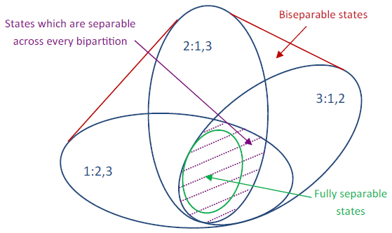
In the multipartite case, the picture becomes even more complex. Indeed, checking separability of a given state across all bipartite splitting of the subsystems is not enough to guarantee that it is fully separable. Motivated by this easy observation, one can define a hierarchy of relaxations of the latter notion: a state on $\mathrm{H}_{1}\otimes\cdots\otimes\mathrm{H}_{k}$ is $\ell$-separable, where $2\leqslant\ell\leqslant k$, if it is a convex combination of states, each of which is separable across a given splitting of the $k$ subsystems into $\ell$ groups (note that, in general, there is no splitting of the $k$ subsystems into $\ell$ groups across which an $\ell$-separable state is separable). $k$-separability is then just full separability, while a state which is not $2$-separable is called genuinely multipartite entangled. These various notions of separability are illustrated in the tripartite case $\mathrm{H}=\mathrm{H}_{1}\otimes\mathrm{H}_{2}\otimes\mathrm{H}_{3}$ in Figure 2.1 (where $x\,{:}\,y,z$ denotes the set of states on $\mathrm{H}$ which are separable across the bipartite cut $\mathrm{H}_{x}{:}\mathrm{H}_{y}\otimes\mathrm{H}_{z}$).

All these notions concerning entanglement detection will be crucial in several places of this manuscript, most notably in Chapters 8 and 9, but also to a lesser extent in Chapters 7 and 10.

Classical information theory is concerned with quantifying the amount of information and correlations present in probability distributions. By analogy, quantum information theory is concerned with doing the same for density operators. We gather here some basic definitions and facts from the quantum Shannon theory that we shall later need here and there. The reader is for instance referred to the book [178], Chapter 11, for a complete expounding of these notions.

The von Neumann entropy of a quantum state $\rho$ is defined as

It is always non-negative, and equal to $0$ if and only if $\rho$ is a pure state. In the case where the underlying Hilbert space $\mathrm{H}$ is finite-dimensional, it is upper-bounded by $\log|\mathrm{H}|$, with equality if and only if $\rho$ is the maximally mixed state $\mathrm{Id}/|\mathrm{H}|$.

The mutual information of a state $\rho$, on a bipartite Hilbert space $\mathrm{H}_{1}\otimes\mathrm{H}_{2}$, is defined as

By sub-additivity of the quantum entropy [5], it is always non-negative, and equal to $0$ if and only if $\rho=\rho_{1}\otimes\rho_{2}$, i.e.  if and only if there is no correlation (not even classical ones) between the two subsystems.

The conditional mutual information of a state $\rho$, on a tripartite Hilbert space $\mathrm{H}_{1}\otimes\mathrm{H}_{2}\otimes\mathrm{H}_{3}$, is defined as

By strong sub-additivity of the quantum entropy [135], it is always non-negative.

Finally, the relative entropy between states $\rho$ and $\sigma$ is defined as

It is always non-negative, and infinite whenever the support of $\rho$ and the orthogonal of the support of $\sigma$ have a non-zero intersection. For a state $\rho$ on a bipartite Hilbert space $\mathrm{H}_{1}\otimes\mathrm{H}_{2}$, we have the notable property that $D(\rho\|\rho_{1}\otimes\rho_{2})=I(\mathrm{H}_{1}{:}\mathrm{H}_{2})(\rho)$.

The main reason why we shall later be interested in these entropic quantities is because several measures of the amount of entanglement present in multipartite quantum systems can be built from them. We will need all these definitions chiefly in Chapters 5 and 10.

Let $\mathrm{H}$ be a Hilbert space and $\{|i\rangle,\ 1\leqslant i\leqslant|\mathrm{H}|\}$ be an orthonormal basis of $\mathrm{H}$ (with the convention that $\{1,\ldots,|\mathrm{H}|\}=\mathbf{N}$ whenever $\mathrm{H}$ is infinite-dimensional). For any $n\in\mathbf{N}$ and any permutation $\pi\in\mathfrak{S}(n)$, denote by $U(\pi)\in\mathcal{U}(\mathrm{H}^{\otimes n})$ the associated permutation unitary on $\mathrm{H}^{\otimes n}$, characterized by

Note that this definition is actually independent of the basis. The $n$-symmetric subspace of $\mathrm{H}^{\otimes n}$ can then be defined as the simultaneous $+1$-eigenspace of all $U(\pi)$’s,

The orthogonal projector onto $\Sym^{n}\left(\mathrm{H}\right)$ may thus be written as

where for each $1\leqslant i_{1}\leqslant\cdots\leqslant i_{n}\leqslant|\mathrm{H}|$, $|\psi_{i_{1},\ldots,i_{n}}\rangle$ denotes the unit vector having same direction as $|v_{i_{1},\ldots,i_{n}}\rangle$. In the case where $\mathrm{H}$ is finite-dimensional, this can also be re-written as

where $\mathrm{d}\psi$ stands for the uniform probability measure on the unit sphere $S_{\mathrm{H}}$ of $\mathrm{H}$. This is due to Schur’s Lemma, since $\Sym^{n}\left(\mathrm{H}\right)$ is an irreducible representation of the commutant action of $\{U(\pi),\ \pi\in\mathfrak{S}(n)\}$, which is that of the local unitaries $\{U^{\otimes n},\ U\in\mathcal{U}(\mathrm{H})\}$ (see e.g. [166] for more group representation background).

A state $\rho$ on $\mathrm{H}^{\otimes n}$ is said to be permutation-invariant if it satisfies $U(\pi)\rho U(\pi)^{\dagger}=\rho$ for all $\pi\in\mathfrak{S}(n)$. This condition is actually equivalent to the existence of a unit vector $|\psi\rangle\in\Sym^{n}\left(\mathrm{H}\otimes\mathrm{H}^{\prime}\right)$, where $\mathrm{H}^{\prime}\equiv\mathrm{H}$, such that $\rho=\tr_{\mathrm{H}^{\prime}}|\psi\rangle\!\langle\psi|$. That is why permutation-invariant states are also sometimes simply referred to as symmetric states.

The permutation-invariant states on $(\mathbf{C}^{d})^{\otimes 2}$ are the so-called Werner states. These are mixtures of the (fully) symmetric state $\pi_{s}$ and the (fully) antisymmetric state $\pi_{a}$ on $(\mathbf{C}^{d})^{\otimes 2}$ (which are defined as the renormalized projectors onto the symmetric and antisymmetric subspaces of $(\mathbf{C}^{d})^{\otimes 2}$, respectively). Concretely, set

We then have the orthogonal direct sum decomposition

The two states $\pi_{s}$ and $\pi_{a}$ on $(\mathbf{C}^{d})^{\otimes 2}$ are therefore defined as

And we define next, for each $0\leqslant\lambda\leqslant 1$, the Werner state $\rho_{\lambda}:=\lambda\pi_{s}+(1-\lambda)\pi_{a}$ on $(\mathbf{C}^{d})^{\otimes 2}$.

This one-parameter family of states was introduced in [177] in order to understand the relation between entanglement and violation of Bell inequalities. It has received considerable interest since then. Indeed, due to their symmetry property, quantities which may be hard to compute in general become much easier to analyze for Werner states. And still, permutation-invariance is an assumption which is more often than not natural to make, so that they encompass a wide enough range of situations. For instance, separability vs entanglement is simple to characterize for Werner states, because it coincides with their being positive under partial transposition or not (see Chapter 2, Section 2.4, for definitions). The result is that $\rho_{\lambda}$ is separable for $1/2\leqslant\lambda\leqslant 1$ and entangled for $0\leqslant\lambda<1/2$ [177].

The motivation behind all de Finetti type theorems is to reduce the study of permutation-invariant scenarios to that of i.i.d. ones. This is precisely what the seminal classical finite de Finetti theorem, proved by Diaconis and Freedman in [60], enables. Indeed, it tells us that the marginal probability distribution (in a few random variables) of an exchangeable probability distribution (in a lot of random variables) is well-approximated by a convex combination of product probability distributions. More precisely, we have the quantitative error-bound provided by Theorem 3.3.1 below.

The first quantum analogue of this result was established by Christandl, König, Mitchison and Renner in [48]. The statement is of similar spirit: the reduced state (on a few subsystems) of a permutation-invariant state (on a lot of subsystems) is well-approximated by a convex combination of product states. Again, the worst-case error can be quantitatively upper-bounded, which is the content of Theorem 3.3.2 below.

Note that the main difference between these two theorems is that the classical one applies to probability distributions on an infinite size alphabet while the quantum one only applies to quantum states on a finite-dimensional Hilbert space. And it is known that the appearance of the dimension in the upper bound is not an artefact of the proof techniques: there actually exist permutation-invariant states $\rho^{(n)}$ on $(\mathbf{C}^{d})^{\otimes n}$ which are such that the distance of $\rho^{(k)}$ to the set of separable states on $(\mathbf{C}^{d})^{\otimes k}$ scales as $kd/n$ (see [48], Section C, or [144], Section III, for such examples).

In Chapter 9, a hierarchy of necessary conditions for separability, based on symmetric extensions, is studied in extensive depth. And it is Theorem 3.3.2 under this precise form which allows to prove that this hierarchy converges to separability. However, in many applications, one does not actually need such a strong approximation result: knowing only that the considered permutation-invariant state can be upper bounded by a convex combination of tensor power states (up to some multiplicative factor $C$) is enough. Indeed, assume that you have such an operator-ordering, and that you know that a given order-preserving linear form $f$ satisfies $f\leqslant\epsilon$, for some $0<\epsilon<1$, on $1$-particle states. Then, you can conclude that $f^{\otimes n}\leqslant C\epsilon^{n}$ on permutation-invariant $n$-particle states, which decays exponentially to $0$ with $n$. These de Finetti results of different kind are usually referred to as de Finetti reductions or post-selection lemmas. Establishing and applying appropriate variants of them is at the heart of Chapters 10 and 11.

The standard convex geometry concepts expounded in this section will be crucial tools in (at least part of) Chapters 6, 7, 8 and 9. The reader is e.g. referred to the lecture notes [20] or [175] for a detailed and accessible presentation.