Another one grinds the dust: Variability of the planetary debris disc at the white dwarf SDSS J104341.53+085558.2
Abstract
We report nine years of optical spectroscopy of the metal-polluted white dwarf SDSS J104341.53+085558.2, which presents morphological variations of the line profiles of the 8600 Å Ca ii triplet emission from the gaseous component of its debris disc. Similar changes in the shape of the Ca ii triplet have also been observed in two other systems that host a gaseous disc, and are likely related to the same mechanism. We report the Mg, Si, and Ca abundances of the debris detected in the photosphere of SDSS J1043+0855, place upper limits on O and Fe, and derive an accretion rate of - gs-1, consistent with those found in other systems with detected debris discs. The Mg/Si ratio and the upper limit on the Fe/Si ratio of the accreted material broadly agree with those found for the crust of the Earth. We also review the range of variability observed among white dwarfs with planetary debris discs.
Keywords:
Stars: individual: SDSS J104341.53+085558.2 – white dwarfs – Circumstellar matter – accretion, accretion discs – line: profiles.1 Introduction
The detection of metal pollution in white dwarf atmospheres provides strong evidence that 25-50 per cent of white dwarfs host remnants of planetary systems (Zuckerman et al., 2003; Koester et al., 2014; Koester & Kepler, 2015). The survival of planets through the post main-sequence evolution of their host star is further supported by the detection of more than 35 dusty debris discs at white dwarfs with metal pollution (Kilic et al., 2006; Farihi et al., 2008; Farihi et al., 2009; Jura et al., 2009; Debes et al., 2011; Hoard et al., 2013; Bergfors et al., 2014; Rocchetto et al., 2015), and is also predicted by theoretical studies (Villaver & Livio, 2007; Veras & Gänsicke, 2015).
Debris discs around white dwarfs are thought to be produced by the tidal disruption of asteroids (or comets) scattered onto a highly eccentric orbit by planets in the system (Graham et al., 1990; Jura, 2003). While recent simulations have begun to explore the formation and evolution of these discs; from the initial disruption of the planetesimal and the shrinking of its orbit (Debes et al., 2012; Veras et al., 2014; Veras et al., 2015), to the dynamics and interactions of the debris within the disc (Rafikov, 2011; Metzger et al., 2012), many aspects remain poorly understood.
Over the last decade, gaseous debris discs have been detected around eight white dwarfs, all of which also host circumstellar dust and have metal polluted photospheres (Gänsicke et al., 2006; Gänsicke et al., 2007; Gänsicke et al., 2008; Gänsicke, 2011; Farihi et al., 2012; Melis et al., 2012; Wilson et al., 2014; Guo et al., 2015). These systems were identified by the detection of Ca ii 8498.02 Å, 8542.09 Å, 8662.14 Å emission lines (henceforth the Ca ii triplet, air wavelengths are given).

| Date | Telescope/Instrument | Wavelength Range [Å] | Resolution [Å] | Exposure Time [s] a |
|---|---|---|---|---|
| 2003 April 05 | SDSS | 3800 – 9200 | 2.9 | 2900 |
| 2007 February 03 | WHT/ISIS | 7400 – 9200 | 2.0 | 4800 |
| 2009 February 16 | WHT/ISIS | 6000 – 8900 | 3.7 | 3950 |
| 2010 April 22 | WHT/ISIS | 8100 – 8850 | 1.1 | 7200 |
| 2011 January 29 | VLT/X-Shooter | 2990 – 10400 | 1.12 | 2950 / 2840 |
| 2011 May 30 | VLT/X-Shooter | 2990 – 10400 | 1.15 | 2950 / 2840 |
| 2012 January 03 | SDSS | 3602 – 10353 | 3.2 | 2702 |
So far only four of these eight gas disc systems have multi-epoch spectroscopy over time scales of years, three of which show variability in the Ca ii emission of the gaseous disc; either as significant changes in the morphology of the Ca ii triplet (Wilson et al., 2015; Manser et al., 2016), or as a decrease in strength of the lines (Wilson et al., 2014). It is thought that the gaseous components of the debris discs in these systems are tracers of dynamic activity (Gänsicke et al., 2008; Wilson et al., 2014; Wilson et al., 2015; Manser et al., 2016).
The gaseous disc around SDSS J104341.53+085558.2 (henceforth SDSS J1043+0855) was discovered by Gänsicke et al. (2007) via the detection of Ca ii triplet emission. An infrared excess was detected by Melis et al. (2010) and Brinkworth et al. (2012), confirming the presence of a dusty disc in SDSS J1043+0855. Here, we report nine years of spectroscopic observations of SDSS J1043+0855 that reveal a change in the morphology of the Ca ii triplet, similar to those seen in other gaseous disc systems (SDSS J122859.93+104032.9 and SDSS J084539.17+225728.0, henceforth SDSS J1228+1040 and SDSS J0845+2257, Wilson et al. 2015; Manser et al. 2016). We also present the accretion rates of the debris onto the white dwarf and the metal abundances of the debris.
2 Observations
We obtained optical spectroscopy of SDSS J1043+0855 from 2003 to 2012 with several instruments: X-Shooter (Vernet et al., 2011) on the ESO Very Large Telescope (VLT); the 2.5 m Sloan Digital Sky Survey telescope (SDSS, data retrieved from DR7 and DR9, Gunn et al. 2006; Abazajian et al. 2009; Eisenstein et al. 2011; Ahn et al. 2014; Smee et al. 2013); and the Intermediate dispersion Spectrograph and Imaging System (ISIS) on the William Herschel Telescope (WHT). A log of the observations is summarised in Table 1. The X-Shooter data were reduced within the reflex †† † Documentation and software for reflex can be obtained from http://www.eso.org/sci/software/reflex/ reduction work flow using the standard settings and optimising the slit integration limits (Freudling et al., 2013). The sky spectrum of each observation was used to determine the spectral resolution. The first ISIS spectrum of SDSS J1043+0855 was reported in Gänsicke et al. (2007), the additional ISIS spectra were obtained with a similar setup, and were reduced in the same fashion (see Farihi et al. 2012 and Wilson et al. 2014 for additional details). We removed the telluric lines present in the VIS arm of the X-Shooter spectra using the X-Shooter Spectral Library (XSL) provided by Chen et al. (2014), and applying the method outlined in Manser et al. (2016).

3 Evolution of the calcium emission profile
3.1 Double peaked emission from a disc
The characteristic emission profile from a gaseous disc with a radially symmetric intensity distribution and circular orbit is a symmetric, double-peaked emission profile (see Figure 1 of Horne & Marsh 1986). The width of the profile arises from the wide range of velocities projected along the line of sight and can reveal details about the structure and geometry of the gaseous disc. The largest velocities correspond to material at the inner disc radius, which can hence be determined from the full width at zero intensity, i.e. the point at which the emission drops to the continuum level, and with knowledge of the inclination, , using , where and denote the actual and observed radii respectively. We define the maximum red/blue-shifted velocities to represent the red/blue inner edges of the disc. The outer radius can be estimated from the peak separation in the double peaked profile.
Any departure from a radially symmetric, circular disc will manifest itself as asymmetries in the double peaked emission profile. An eccentric disc of uniform intensity, for example, would generate an asymmetric double-peaked profile if viewed along the semi-minor axis, as there is an asymmetry in the velocity distribution of the material, as well as in the total red and blue-shifted light emitted from the disc. We use this insight below to discuss the changes in the line profiles observed at SDSS J1043+0855.
3.2 Variation of the Calcium emission lines
The Ca ii triplet in SDSS J1043+0855 changes in morphology over a time scale of nine years (Figure 2). All three components of the triplet vary in the same manner and are henceforth referred to in singular.
The initial three spectra are noisy and of low resolution, showing a broad line profile. In contrast, finer features appear in the higher resolution 2010 WHT spectrum, namely a sharp red-shifted peak and a gradual drop off to blueward wavelengths, revealing a clear asymmetry in the red and blue inner edges of the disc. This asymmetry decreases in the 2011 January spectrum, and vanishes in the 2011 May spectrum. The second SDSS spectrum obtained in 2012 shows no sign of any sharp departures from symmetry, although it is of relatively low spectral resolution. In Section 5 we discuss the similarities, and the possible origin, of the observed variations with those seen in other systems.
3.3 Inclination of the disc
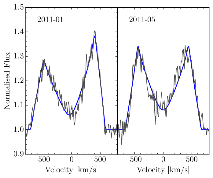
In the 2011 January and May spectra, the ‘valley’ in between the two peaks of the emission profiles almost reaches the continuum level, which suggests that the debris disc is optically thick and seen at a large inclination. Horne & Marsh (1986) have shown that in an optically thick accretion disc, line emission is more likely to escape along paths of largest velocity gradient provided by Keplerian shear flow, which is at a minimum for purely tangential or radial emission through the disc. For an observer looking through the disc at an inclination of 90∘ (edge on), material travelling perpendicular to the line of sight (emission in the ‘valley’) will be emitting along the radial direction of the disc and will therefore be suppressed.
While the formulation described in Horne & Marsh (1986) was developed for circular orbits, it was expanded to include eccentric orbits in order to model the emission profile of SDSS J1228+1040 obtained in 2006 (Gänsicke et al., 2006), and we give additional details on this extension in Appendix A. We fit the emission profiles of the 2011 January and May spectra of SDSS J1043+0855 in the same manner (see Figure 3), and obtain an inclination of 76∘ and 72∘ respectively, leading to an average inclination of 74∘. The statistical uncertainty obtained for the two inclinations was 0.5∘, which is probably an underestimate, and a more realistic uncertainty is taken to be 5∘.
4 Metal abundances in the photosphere of SDSS J1043+0855
We fitted the two SDSS spectra with DA (hydrogen dominated) white dwarf model atmospheres using the methods described in Gänsicke et al. (2012) and Koester et al. (2014), and find = 17879 195 K, and = 8.124 0.033, corresponding to = 0.693 0.020 and = 0.0120 0.0003 (see Table 2). Using the initial-to-final mass relation of Casewell et al. (2009), Kalirai et al. (2008), Catalán et al. (2008), and Williams et al. (2009), we estimate the mass of the white dwarf progenitor to be 2.76 0.04 .
We note that while the atmospheric parameters derived here are consistent with previous measurements (Eisenstein et al., 2006; Gänsicke et al., 2007; Tremblay et al., 2011; Kleinman et al., 2013) the photometry suggests a lower effective temperature, even when allowing for the maximum reddening along the line of sight obtained from Schlafly & Finkbeiner (2011). This discrepancy is likely due to a higher amount of extinction, either by a denser patch in the interstellar medium that remains unresolved in the dust maps, or by circumstellar dust. We speculate that there could be additional dust in the system, which may not be associated with the dusty component of the debris disc at SDSS J1043+0855 (Melis et al., 2010; Brinkworth et al., 2012), and could possibly be the cause of the observed reddening.
| Name | Type | Features | ref | |||||
| (g cm-2) | (K) | () | (Myr) | ( g s-1) | ||||
| SDSS J0738+1835 | DB | 8.4 (0.2) | 13950 (100) | 0.841 (0.131) | 477 (160) | e | 1 | |
| SDSS J0845+2257 | DB | 8.18 (0.20) | 19780 (250) | 0.73 (0.11) | 122 (44) | e, v | 2 | |
| SDSS J0959–0200 | DA | 8.06 (0.03) | 13280 (20) | 0.64 (0.02) | 324 (17) | e, v | 3, 4 | |
| SDSS J1043+0855 | DA | 8.124 (0.033) | 17879 (195) | 0.693 (0.020) | 153 (10) | (2.5 - 12) | e, v | 5, 6, 7 |
| WD 1144+0529 | DA | 7.74 (0.03) | 23027 (219) | 0.49 (0.03) | 21.2 (1.9) | - | e | 8 |
| SDSS J1228+1040 | DA | 8.150 (0.089) | 20713 (281) | 0.705 (0.051) | 100 (5) | e, a, v | 6, 9, 10, 11, 12 | |
| HE 1349–2305 | DA | 8.133 | 18173 | 0.673 | 149.4 | e | 13, 14, 15 | |
| SDSS J1617+1620 | DA | 8.11 (0.08) | 13520 (200) | 0.68 (0.05) | 350 (50) | - | e, v | 16 |
| PG 0843+516 | DA | 7.902 (0.089) | 22412 (304) | 0.577 (0.047) | 42 (4) | a | 11 | |
| WD 1054–226 | DA | 8.04 (0.03) | 7903 (16) | - | 1255 (92) | - | a | 17 |
| WD 1124–293 | DA | 8.1 | 9700 | 0.66 | 843 | a | 18, 19 | |
| WD 1145+017 | DB | - | 15900 (500) | - | 175 (75) | a, v | 20, 21 |
| Element | [h] | [g s-1] | Bulk Earth mass fraction [per cent] a | Inferred total [g s-1] | |
|---|---|---|---|---|---|
| 8 O | 65.0 | 32.4 | |||
| 12 Mg | (0.15) | 26.5 | 15.8 | ||
| 14 Si | (0.15) | 13.8 | 17.1 | ||
| 20 Ca | (0.20) | 18.6 | 1.6 | ||
| 26 Fe | 11.1 | 28.8 |
Using the system parameters, the metal absorption lines detected in the spectra of SDSS J1043+0855 were modelled (see Figure 4) to measure abundances relative to hydrogen which are given in Table 3, along with the diffusion time scales and accretion fluxes. The abundance by number of Mg, Ca, and an upper limit for Fe relative to Si were found to be (Mg/Si) = , (Ca/Si) = , and (Fe/Si) . From Figure 7 of Jura & Young (2014), the ratios of Mg and Fe to Si are broadly consistent with those found for the crust of the Earth, and imply the accreted object is processed rather than having a ’chondritic’ composition (Zuckerman et al., 2007; Xu et al., 2013; Xu et al., 2014). This is also supported by the relatively low number abundance of Mg with respect to Ca, (Mg/Ca) = , when compared to a sample of 60 externally polluted white dwarfs (see Figure 1 of Jura & Xu 2013). Similarly low (Mg/Ca) ratios have also observed at other white dwarfs that are thought to accrete crust material, such as NLTT 43806 and NLTT 19868 (Zuckerman et al., 2011; Kawka & Vennes, 2016).
We also note that the Ca K 3934 Å feature shows clear emission in the averaged, normalised X-Shooter spectra (Figure 4). Similar emission is seen at SDSS J1228+1040, which also revealed a difference in morphology between the Ca H & K profiles and the Ca ii triplet, although the signal-to-noise of the current SDSS 1043+0855 spectra is not high enough to determine this (Manser et al., 2016).
We estimate the total accretion rate for each element from the mass flow rates given in Table 3, assuming a bulk Earth composition and the respective mass fractions of each element (from Allègre et al. 2001). The resulting range from Mg, Si, and Ca, gs-1, reflects the uncertainty in the bulk abundances of the planetary debris, but agrees well with the distribution of accretion rates inferred for 19 other metal-polluted DA white dwarfs with dusty discs (Bergfors et al., 2014). For reference, the total accretion rate of SDSS J1228+1040 (where accretion fluxes for all major elements were measured from HST/COS ultraviolet spectra) is (Gänsicke et al., 2012).

| Date | Equivalent width [Å] |
|---|---|
| 2003–04 | -27 (3) |
| 2007–02 | -22 (1) |
| 2009–02 | -15 (1) |
| 2010–04 | -13 (1) |
| 2011–01 | -18 (1) |
| 2011–05 | -20 (1) |
| 2012–01 | -19 (1) |
5 Discussion
Up until the last decade, debris discs around white dwarfs have appeared static in nature, with no significant detections of variability in the properties of the disc itself or in the strength of the absorption lines in metal polluted systems. Due to the short diffusion time scales at the majority of these systems (Koester et al., 2014), any change in the strength of the absorption lines would imply a change in the accretion rate onto the white dwarf. von Hippel & Thompson (2007) claimed changes in the equivalent width of the photospheric Ca ii K line over a time scale of days at GD 29–38, however additional observations obtained by Debes & López-Morales (2008) did not confirm such variation, and they concluded further data were required to determine the possible variable nature of the accretion onto the white dwarf.
In recent years, the spectroscopic monitoring of gaseous discs has revealed variability that gives us insight into their formation and dynamics. Table 2 lists the stellar parameters of the eight published gas disc systems. Other than SDSS J1043+0855, there are four gaseous disc systems with multi-epoch spectroscopy: SDSS J161717.04+162022.4 (Wilson et al. 2014, henceforth SDSS J1617+1620), SDSS J0845+2257 (Gänsicke et al., 2008; Wilson et al., 2015), SDSS J1228+1040 (Manser et al., 2016), and SDSS J073842.56+183509.6 (Gänsicke 2011; Dufour et al. 2012, henceforth SDSS J0738+1835).
SDSS J0845+2257, SDSS J1228+1040, and SDSS J1617+1620 all show variations on a time scale of years, but follow two distinct types of evolution. In SDSS J1617+1620 the Ca ii triplet emission gradually decreased in strength over a time scale of eight years while not undergoing noticeable changes in the line profile shape (Wilson et al., 2014). In contrast, the changes seen in SDSS J0845+2257 and SDSS J1228+1040 are of a morphological nature, analogous to the changes we present here for SDSS J1043+0855. Table 4 lists the equivalent widths (subject to systematic uncertainties related to the method used in continuum fitting, as well as the statistical uncertainties given in Table 4) of the Ca ii emission lines in SDSS J1043+0855, which do not show any long term decay of the equivalent width of the Ca ii triplet such as seen at SDSS J1617+1620. Only SDSS J0738+1835 has displayed no changes in the shape and strength of the Ca ii triplet over a period of six years, although only three epochs are available, with two of them spaced only a year apart.
Manser et al. (2016) showed that the variable Ca ii triplet line profiles of SDSS J1228+1040 could be interpreted as the emission from a fixed intensity pattern that precesses over a time scale of decades, possibly indicating a young debris disc that still has eccentric orbits and has not fully circularised. General relativistic precession will cause the debris to precess with a radially dependent period, causing orbits to cross one another and inducing collisions which produces the observed gaseous component to the debris disc.
While the evolution of the emission from SDSS J1043+0855 appears to be remarkably similar to SDSS J1228+1040 and SDSS J0845+2257, the data have a lower signal to noise and have fewer epochs, and thus, while it is likely that the same physical mechanism is responsible for the evolution of the line profiles observed in all three systems, regular spectroscopic monitoring of all gas discs is necessary to develop a more detailed understanding of the dynamical processes present in planetary debris discs around white dwarfs.
Variability of debris discs is not only limited to the Ca ii triplet line profile. The dusty disc around SDSS J0959–0200 was observed to significantly decrease in infrared flux by Xu & Jura (2014), who propose two mechanisms by which the disc could be depleted; a recent planetesimal impact on the disc, or instability near the inner edge. We suggest an additional scenario of a vertically extended cloud of dust, generated from an asteroid colliding with a pre-existing disc (Jura, 2008). Such an optically thin cloud would temporarily add to the infrared emission of the optically thick disc, but the overall infrared emission from the system would decrease as the dust cloud settled into the disc.
In Table 2 we also include four additional systems where circumstellar absorption of gaseous material has been detected around the host white dwarf, including WD 1145+017, which is orbited by highly-dynamic debris, transiting the white dwarf with periods of 4.5 hr (Vanderburg et al., 2015; Xu et al., 2016; Gänsicke et al., 2016; Rappaport et al., 2016). WD 1145+017 is unequivocally a highly dynamical and evolving system with a planetesimal currently undergoing disruption, and also hosts circumstellar gas absorption (Xu et al., 2016). Curiously, the detection of absorption due to circumstellar gas does not correlate with the presence of Ca ii triplet emission: SDSS 1228+1040 is so far the only system in which both have been detected (Gänsicke et al., 2012). We note that circumstellar gas has been detected also around a number of hot and young white dwarfs, their origin is probably diverse in nature and not unambiguously associated with evolved planetary systems (Dickinson et al., 2012; Barstow et al., 2014).
6 Conclusions
We report here the morphological variability of the Ca ii triplet in SDSS J1043+0855 on a time scale of nine years. The evolution of the Ca ii triplet reported here is similar to that of two other systems, SDSS J1228+1040 and SDSS J0845+2257.
We have also analysed the optical spectra of SDSS J1043+0855 to determine its stellar parameters and the photospheric metal abundance. The Mg/Si and (upper limit to the) Fe/Si ratios of the planetary debris that has been accreted onto the white dwarf are broadly consistent with those of the crust of the Earth.
The recent detection of the ’real time’ disruption of a planetesimal at WD 1145+017, along with the dynamical evolution seen at the gaseous discs SDSS J1043+0855, SDSS J1228+1040, SDSS J1617+1620, and SDSS J0845+2257 reveals that variability at planetary systems around white dwarfs is more common than was initially thought. Additional spectroscopic and photometric monitoring of all the gaseous discs known so far is key to developing a more detailed understanding of the dynamical processes present in planetary debris discs at white dwarfs.
Acknowledgements
The research leading to these results has received funding from the European Research Council under the European Union’s Seventh Framework Programme (FP/2007-2013) / ERC Grant Agreement n. 320964 (WDTracer). We would like to thank Yan-Ping Chen and Scott Trager for sharing their X-Shooter telluric template library. We thank the anonymous referee for a timely and constructive report.
Based on observations made with ESO Telescopes at the La Silla Paranal Observatory under programme IDs: 087.D-0139 and 386.C-0218. This work has made use of observations from the SDSS-III, funding for which has been provided by the Alfred P. Sloan Foundation, the Participating Institutions, the National Science Foundation, and the U.S. Department of Energy Office of Science. The SDSS-III web site is http://www.sdss3.org/. Based on observations made with the WHT operated on the island of La Palma by the Isaac Newton Group in the Spanish Observatorio del Roque de los Muchachos of the Instituto de Astrofísica de Canarias.
References
- Abazajian et al. (2009) Abazajian K. N., et al., 2009, ApJS, 182, 543
- Ahn et al. (2014) Ahn C. P., et al., 2014, ApJ, 211, 17
- Allègre et al. (2001) Allègre C., Manhès G., Lewin E., 2001, Earth and Planetary Science Letters, 185, 49
- Barstow et al. (2014) Barstow M. A., Barstow J. K., Casewell S. L., Holberg J. B., Hubeny I., 2014, MNRAS, 440, 1607
- Bergfors et al. (2014) Bergfors C., Farihi J., Dufour P., Rocchetto M., 2014, MNRAS, 444, 2147
- Brinkworth et al. (2012) Brinkworth C. S., Gänsicke B. T., Girven J. M., Hoard D. W., Marsh T. R., Parsons S. G., Koester D., 2012, ApJ, 750, 86
- Casewell et al. (2009) Casewell S. L., Dobbie P. D., Napiwotzki R., Burleigh M. R., Barstow M. A., Jameson R. F., 2009, MNRAS, 395, 1795
- Catalán et al. (2008) Catalán S., Isern J., García-Berro E., Ribas I., Allende Prieto C., Bonanos A. Z., 2008, A&A, 477, 213
- Chen et al. (2014) Chen Y.-P., Trager S. C., Peletier R. F., Lançon A., Vazdekis A., Prugniel P., Silva D. R., Gonneau A., 2014, A&A, 565, A117
- Debes & López-Morales (2008) Debes J. H., López-Morales M., 2008, ApJ Lett., 677, L43
- Debes et al. (2011) Debes J. H., Hoard D. W., Wachter S., Leisawitz D. T., Cohen M., 2011, ApJS, 197, 38
- Debes et al. (2012) Debes J. H., Walsh K. J., Stark C., 2012, ApJ, 747, 148
- Dickinson et al. (2012) Dickinson N. J., Barstow M. A., Welsh B. Y., Burleigh M., Farihi J., Redfield S., Unglaub K., 2012, MNRAS, 423, 1397
- Dufour et al. (2012) Dufour P., Kilic M., Fontaine G., Bergeron P., Melis C., Bochanski J., 2012, ApJ, 749, 6
- Eisenstein et al. (2006) Eisenstein D. J., et al., 2006, ApJS, 167, 40
- Eisenstein et al. (2011) Eisenstein D. J., et al., 2011, AJ, 142, 72
- Farihi et al. (2008) Farihi J., Zuckerman B., Becklin E. E., 2008, ApJ, 674, 431
- Farihi et al. (2009) Farihi J., Jura M., Zuckerman B., 2009, ApJ, 694, 805
- Farihi et al. (2012) Farihi J., Gänsicke B. T., Steele P. R., Girven J., Burleigh M. R., Breedt E., Koester D., 2012, MNRAS, 421, 1635
- Freudling et al. (2013) Freudling W., Romaniello M., Bramich D. M., Ballester P., Forchi V., García-Dabló C. E., Moehler S., Neeser M. J., 2013, A&A, 559, A96
- Gänsicke (2011) Gänsicke B. T., 2011, in Schuh S., Drechsel H., Heber U., eds, American Institute of Physics Conference Series Vol. 1331, American Institute of Physics Conference Series. pp 211–214 (arXiv:1101.3946), doi:10.1063/1.3556202
- Gänsicke et al. (2006) Gänsicke B. T., Marsh T. R., Southworth J., Rebassa-Mansergas A., 2006, Science, 314, 1908
- Gänsicke et al. (2007) Gänsicke B. T., Marsh T. R., Southworth J., 2007, MNRAS, 380, L35
- Gänsicke et al. (2008) Gänsicke B. T., Koester D., Marsh T. R., Rebassa-Mansergas A., Southworth J., 2008, MNRAS, 391, L103
- Gänsicke et al. (2012) Gänsicke B. T., Koester D., Farihi J., Girven J., Parsons S. G., Breedt E., 2012, MNRAS, 424, 333
- Gänsicke et al. (2016) Gänsicke B. T., et al., 2016, ApJ, 818, L7
- Graham et al. (1990) Graham J. R., Matthews K., Neugebauer G., Soifer B. T., 1990, ApJ, 357, 216
- Gunn et al. (2006) Gunn J. E., et al., 2006, AJ, 131, 2332
- Guo et al. (2015) Guo J., Tziamtzis A., Wang Z., Liu J., Zhao J., Wang S., 2015, ApJ, 810, L17
- Hoard et al. (2013) Hoard D. W., Debes J. H., Wachter S., Leisawitz D. T., Cohen M., 2013, ApJ, 770, 21
- Horne & Marsh (1986) Horne K., Marsh T. R., 1986, MNRAS, 218, 761
- Jura (2003) Jura M., 2003, ApJ Lett., 584, L91
- Jura (2008) Jura M., 2008, AJ, 135, 1785
- Jura & Xu (2013) Jura M., Xu S., 2013, ApJ, 145, 30
- Jura & Young (2014) Jura M., Young E. D., 2014, Annual Review of Earth and Planetary Sciences, 42, 45
- Jura et al. (2009) Jura M., Farihi J., Zuckerman B., 2009, AJ, 137, 3191
- Kalirai et al. (2008) Kalirai J. S., Hansen B. M. S., Kelson D. D., Reitzel D. B., Rich R. M., Richer H. B., 2008, ApJ, 676, 594
- Kawka & Vennes (2016) Kawka A., Vennes S., 2016, MNRAS, 458, 325
- Kilic et al. (2006) Kilic M., von Hippel T., Leggett S. K., Winget D. E., 2006, ApJ, 646, 474
- Kleinman et al. (2013) Kleinman S. J., et al., 2013, ApJS, 204, 5
- Koester & Kepler (2015) Koester D., Kepler S. O., 2015, A&A, 583, A86
- Koester & Wilken (2006) Koester D., Wilken D., 2006, A&A, 453, 1051
- Koester et al. (2005) Koester D., Rollenhagen K., Napiwotzki R., Voss B., Christlieb N., Homeier D., Reimers D., 2005, A&A, 432, 1025
- Koester et al. (2014) Koester D., Gänsicke B. T., Farihi J., 2014, A&A, 566, A34
- Manser et al. (2016) Manser C. J., et al., 2016, MNRAS, 455, 4467
- Melis et al. (2010) Melis C., Jura M., Albert L., Klein B., Zuckerman B., 2010, ApJ, 722, 1078
- Melis et al. (2012) Melis C., et al., 2012, ApJ Lett., 751, L4
- Metzger et al. (2012) Metzger B. D., Rafikov R. R., Bochkarev K. V., 2012, MNRAS, 423, 505
- Rafikov (2011) Rafikov R. R., 2011, MNRAS, 416, L55
- Rappaport et al. (2016) Rappaport S., Gary B. L., Kaye T., Vanderburg A., Croll B., Benni P., Foote J., 2016, MNRAS,
- Rocchetto et al. (2015) Rocchetto M., Farihi J., Gänsicke B. T., Bergfors C., 2015, MNRAS, 449, 574
- Schlafly & Finkbeiner (2011) Schlafly E. F., Finkbeiner D. P., 2011, ApJ, 737, 103
- Smee et al. (2013) Smee S. A., et al., 2013, AJ, 146, 32
- Tremblay et al. (2011) Tremblay P.-E., Bergeron P., Gianninas A., 2011, ApJ, 730, 128
- Vanderburg et al. (2015) Vanderburg A., et al., 2015, Nature, 526, 546
- Vennes & Kawka (2013) Vennes S., Kawka A., 2013, ApJ, 779, 70
- Veras & Gänsicke (2015) Veras D., Gänsicke B. T., 2015, MNRAS, 447, 1049
- Veras et al. (2014) Veras D., Leinhardt Z. M., Bonsor A., Gänsicke B. T., 2014, MNRAS, 445, 2244
- Veras et al. (2015) Veras D., Leinhardt Z. M., Eggl S., Gänsicke B. T., 2015, MNRAS, 451, 3453
- Vernet et al. (2011) Vernet J., et al., 2011, A&A, 536, A105
- Villaver & Livio (2007) Villaver E., Livio M., 2007, ApJ, 661, 1192
- Voss et al. (2007) Voss B., Koester D., Napiwotzki R., Christlieb N., Reimers D., 2007, A&A, 470, 1079
- Williams et al. (2009) Williams K. A., Bolte M., Koester D., 2009, ApJ, 693, 355
- Wilson et al. (2014) Wilson D. J., Gänsicke B. T., Koester D., Raddi R., Breedt E., Southworth J., Parsons S. G., 2014, MNRAS, 445, 1878
- Wilson et al. (2015) Wilson D. J., Gänsicke B. T., Koester D., Toloza O., Pala A. F., Breedt E., Parsons S. G., 2015, MNRAS, 451, 3237
- Xu & Jura (2014) Xu S., Jura M., 2014, ApJ, 792, L39
- Xu et al. (2013) Xu S., Jura M., Klein B., Koester D., Zuckerman B., 2013, ApJ, 766, 132
- Xu et al. (2014) Xu S., Jura M., Koester D., Klein B., Zuckerman B., 2014, ApJ, 783, 79
- Xu et al. (2016) Xu S., Jura M., Dufour P., Zuckerman B., 2016, ApJ, 816, L22
- Zuckerman et al. (2003) Zuckerman B., Koester D., Reid I. N., Hünsch M., 2003, ApJ, 596, 477
- Zuckerman et al. (2007) Zuckerman B., Koester D., Melis C., Hansen B. M., Jura M., 2007, ApJ, 671, 872
- Zuckerman et al. (2011) Zuckerman B., Koester D., Dufour P., Melis C., Klein B., Jura M., 2011, ApJ, 739, 101
- von Hippel & Thompson (2007) von Hippel T., Thompson S. E., 2007, ApJ, 661, 477
Appendix A Velocities and velocity gradients in an eccentric disc
Horne & Marsh (1986) show that line photons travelling through an optically thick disc are more likely to escape along paths of the greatest velocity gradient. We derive and list here the equations needed to calculate the radial velocity and velocity gradient at any point in an elliptical disc of constant orbital eccentricity, and constant orientation of its semi-major axes, . This expands the formulation for modelling emission line profiles from circular discs described by Horne & Marsh (1986). We first set up the basic components of an eccentric orbit, of which some are shown in Figure 5.
A.1 Equations of an elliptical orbit
The polar equation for an ellipse is given as
| (1) |
where is the semi-latus rectum, and is the angle measured from the point of periastron, usually called the “true anomaly”. Conservation of angular momentum in a central force field means that
| (2) |
where , the specific angular momentum, is constant. This therefore leads to the true anomaly as a function of time being determined by the following equation
| (3) |
Making the substitution and setting
| (4) |
where is the eccentric anomaly (see Figure 5), we get
| (5) |
When , we get and , so then we can write
| (6) |
where is the mean angular velocity and is given by
| (7) |

Equation 6 is Kepler’s equation of elliptical motion and can easily be solved numerically, and the true anomaly, , follows from
| (8) |
can be constructed geometrically by putting a circle radius centred on the ellipse, and drawing a line perpendicular to the major axis through any point on the ellipse. The angle subtended by the point on the circle where the perpendicular line cuts it is . Using this, or the above equation, one can show that
| (9) |
Since and always lie within the same range; to or to , this equation is sufficient to determine . Related useful expressions are
| (10) | |||||
| (11) |
Assuming that the ellipse is oriented with the focus at the origin and the semi-major axis parallel to the -axis (pointing left so that the periastron lies on the positive -axis giving the standard orientation for in 2D polar coordinates, see Figure 5), then the velocity at any point is given by
| (12) | |||||
| (13) |
where
| (14) |
and
| (15) |
where
| (16) |
and
| (17) |
The equation for can be reduced to
| (18) |
or, equivalently,
| (19) |
giving the following alternative expressions for the two components of velocity (radial and azimuthal)
| (20) |
and
| (21) |
We are now in a position to consider orbits and radial velocities, and their derivatives.
A.2 Velocity gradients in a confocal elliptical flow
If a point in the disc is viewed by an observer at angle defined so that when looking along the positive -axis and increasing anti-clockwise (see Figure A), then its radial velocity is given by
| (22) |
Horne & Marsh (1986) showed that the velocity gradient is also required to fully model the emission profile of an accretion disc, which using the notation , is given by
| (23) | |||||
| (24) |
| (25) | |||||
| (26) | |||||
| (27) | |||||
| (28) |
One can show that
| (29) | |||||
| (30) |
| (31) | |||||
| (32) | |||||
| (33) | |||||
| (34) |
From Equation 1 we can obtain,
| (35) | |||||
| (36) |
where
| (37) | |||||
| (38) |
and from Kepler’s third law, assuming the mass of the orbiting material to be negligible,
| (39) |
where is the gravitational constant and is the mass of the host star, we finally get the last unknowns,
| (40) | |||||
| (41) |
which now allows one to calculate the velocity derivatives.