跳到论文正文
W Papers独立论文阅读器 arXiv:1607.06534 论文正文 计算阅读时间 · 0%
引用这篇论文根据当前论文元数据生成,正式投稿前建议核对。


License: arXiv.org perpetual non-exclusive license
arXiv:1607.06534v3 [stat.ML] 14 Jan 2017

The Landscape of Empirical Risk for Non-convex Losses

Song Mei Note: Institute for Computational and Mathematical Engineering, Stanford University    Yu Bai Note: Department of Statistics, Stanford University    Andrea Montanari Note: Department of Electrical Engineering and Department of Statistics, Stanford University
Abstract

Most high-dimensional estimation and prediction methods propose to minimize a cost function (empirical risk) that is written as a sum of losses associated to each data point (each example). In this paper we focus on the case of non-convex losses, which is practically important but still poorly understood. Classical empirical process theory implies uniform convergence of the empirical (or sample) risk to the population risk. While –under additional assumptions– uniform convergence implies consistency of the resulting M-estimator, it does not ensure that the latter can be computed efficiently.

In order to capture the complexity of computing M-estimators, we propose to study the landscape of the empirical risk, namely its stationary points and their properties. We establish uniform convergence of the gradient and Hessian of the empirical risk to their population counterparts, as soon as the number of samples becomes larger than the number of unknown parameters (modulo logarithmic factors). Consequently, good properties of the population risk can be carried to the empirical risk, and we are able to establish one-to-one correspondence of their stationary points. We demonstrate that in several problems such as non-convex binary classification, robust regression, and Gaussian mixture model, this result implies a complete characterization of the landscape of the empirical risk, and of the convergence properties of descent algorithms.

We extend our analysis to the very high-dimensional setting in which the number of parameters exceeds the number of samples, and provide a characterization of the empirical risk landscape under a nearly information-theoretically minimal condition. Namely, if the number of samples exceeds the sparsity of the unknown parameters vector (modulo logarithmic factors), then a suitable uniform convergence result takes place. We apply this result to non-convex binary classification and robust regression in very high-dimension.

1 Introduction

M-estimation is arguably the most popular approach to high-dimensional estimation. Given data-points {𝒛1,𝒛2,…,𝒛n}\{{\bm{z}}_{1},{\bm{z}}_{2},\dots,{\bm{z}}_{n}\}, 𝒛i∈ℝd{\bm{z}}_{i}\in{\mathbb{R}}^{d}, we estimate a parameter vector 𝜽∈ℝp{\bm{\theta}}\in{\mathbb{R}}^{p} via

𝜽^n\displaystyle\hat{\bm{\theta}}_{n} =arg⁡min𝜽∈Θn,p​R^n​(𝜽),\displaystyle=\arg\min_{{\bm{\theta}}\in\Theta_{n,p}}\widehat{R}_{n}({\bm{\theta}})\,, (1)
R^n​(𝜽)\displaystyle\widehat{R}_{n}({\bm{\theta}}) ≡1n​∑i=1nℓ⁡(𝜽,𝒛i).\displaystyle\equiv\frac{1}{n}\sum_{i=1}^{n}\ell({\bm{\theta}};{\bm{z}}_{i})\,. (2)

Here ℓ:ℝp×ℝd→ℝ\ell:{\mathbb{R}}^{p}\times{\mathbb{R}}^{d}\to{\mathbb{R}} is a loss function, and Θn,p\Theta_{n,p} is a constraint set. Prominent examples of this general framework include maximum likelihood (ML) estimation [Fis22] and empirical risk minimization [Vap98].

Once the objective (1) is formed, it remains to define a computationally efficient scheme to approximate it. Gradient descent is the most frequently applied idea. Assuming –for the moment– Θn,p=ℝp\Theta_{n,p}={\mathbb{R}}^{p}, this takes the form

𝜽^n(k+1)=𝜽^n(k)−hk∇R^n(𝜽^n(k)).\displaystyle\hat{\bm{\theta}}_{n}(k+1)=\hat{\bm{\theta}}_{n}(k)-h_{k}\,\nabla\widehat{R}_{n}(\hat{\bm{\theta}}_{n}(k))\,. (3)

While a large number of variants and refinements have been developed over the years (projected gradient, accelerated gradient [Nes13b], stochastic gradient [RM51], distributed gradient [TBA84], and so on), these share many of the strengths and weaknesses of the elementary iteration (3).

If gradient descent is adopted, the only freedom is in the choice of the loss function ℓ⁡(⋅,⋅)\ell(\,\cdot\,;\,\cdot\,). Convexity has been a major guiding principle in this respect. If the function ℓ⁡(⋅,𝒛):ℝp→ℝ\ell(\,\cdot\,;{\bm{z}}):{\mathbb{R}}^{p}\to{\mathbb{R}} is convex, then the empirical risk R^n​(⋅)\widehat{R}_{n}(\,\cdot\,) is convex as well and hence gradient descent is globally convergent to an M-estimator (the latter is unique under strict convexity). Also, strong convexity of R^n​(⋅)\widehat{R}_{n}(\,\cdot\,) can be used to prove optimal statistical guarantees for the M-estimator 𝜽^n\hat{\bm{\theta}}_{n}. This line of thought can be traced back as far as Fisher’s argument for the asymptotic efficiency of maximum likelihood estimators [Fis22, Fis25], and originated many beautiful contributions. In recent years, a flourishing line of research addresses the very high-dimensional regime p≫np\gg n, by leveraging on suitable restricted strong convexity assumptions [CT05, CT07, BRT09, NRWY12].

Despite these successes, many problems of practical interest call for non-convex loss functions. Let us briefly mention a few examples of non-convex M-estimators that are often preferred by practitioners to their convex counterparts. We will revisit these examples in Section 4.

In binary linear classification we are given nn pairs 𝒛1=(y1,𝒙1),…,𝒛n=(yn,𝒙n){\bm{z}}_{1}=(y_{1},{\bm{x}}_{1}),\dots,{\bm{z}}_{n}=(y_{n},{\bm{x}}_{n}) with yi∈{0,1}y_{i}\in\{0,1\}, 𝒙i∈ℝd{\bm{x}}_{i}\in{\mathbb{R}}^{d}, and would like to learn a model of the form ℙ⁡(Yi=1|𝑿i=𝒙)=σ⁡(⟨𝜽0,𝒙⟩){\mathbb{P}}(Y_{i}=1|{\bm{X}}_{i}={\bm{x}})=\sigma(\langle{\bm{\theta}}_{0},{\bm{x}}\rangle) with 𝜽0∈ℝd{\bm{\theta}}_{0}\in{\mathbb{R}}^{d} a parameter vector and σ:ℝ→[0,1]\sigma:{\mathbb{R}}\to[0,1] a threshold function. The non-linear square loss ℓ⁡(𝜽,y,𝒙)=(y−σ⁡(⟨𝜽,𝒙⟩))2\ell({\bm{\theta}};y,{\bm{x}})=(y-\sigma(\langle{\bm{\theta}},{\bm{x}}\rangle))^{2} is commonly used in practice

R^n​(𝜽)≡1n​∑i=1n(yi−σ⁡(⟨𝜽,𝒙i⟩))2.\widehat{R}_{n}({\bm{\theta}})\equiv\frac{1}{n}\sum_{i=1}^{n}\Big(y_{i}-\sigma(\langle{\bm{\theta}},{\bm{x}}_{i}\rangle)\Big)^{2}\,. (4)

Several empirical studies [CDT+09, WL12, NS13] demonstrate superior robustness and classification accuracy of non-convex losses in contrast to convex losses (e.g. hinge or logistic loss). The same loss function is commonly used used in neural-network models [LBH15].

A similar scenario arises in robust regression. In this case, we are given nn pairs 𝒛1=(y1,𝒙1){\bm{z}}_{1}=(y_{1},{\bm{x}}_{1}),…,𝒛n=(yn,𝒙n){\bm{z}}_{n}=(y_{n},{\bm{x}}_{n}) with yi∈ℝy_{i}\in{\mathbb{R}}, 𝒙i∈ℝd{\bm{x}}_{i}\in{\mathbb{R}}^{d}, and we assume the linear model yi=⟨𝜽0,𝒙i⟩+εiy_{i}=\langle{\bm{\theta}}_{0},{\bm{x}}_{i}\rangle+\varepsilon_{i}, where the noise terms εi\varepsilon_{i} are i.i.d. with mean zero. Since Huber’s seminal work [Hub73], M-estimators are the method of choice for this problem:

R^n​(𝜽)≡1n​∑i=1nρ⁡(yi−⟨𝜽,𝒙i⟩).\widehat{R}_{n}({\bm{\theta}})\equiv\frac{1}{n}\sum_{i=1}^{n}\rho\big(y_{i}-\langle{\bm{\theta}},{\bm{x}}_{i}\rangle\big)\,. (5)

Robustness naturally suggests to investigate the use of a non-convex function ρ:ℝ→ℝ\rho:{\mathbb{R}}\to{\mathbb{R}}, either bounded or increasing slowly at infinity.

Finally, missing data problems famously lead to non-convex optimization formulations. Consider for instance a mixture-of-Gaussians problems in which we are given data points 𝒛1,…,𝒛n∈ℝd{\bm{z}}_{1},\dots,{\bm{z}}_{n}\in{\mathbb{R}}^{d}, 𝒛i∼∑a=1ki​i​d⁡pa​𝖭​(𝜽a,Id×d){\bm{z}}_{i}\sim_{iid}\sum_{a=1}^{k}p_{a}{\sf N}({\bm{\theta}}_{a},{\rm I}_{d\times d}) (for the sake of simplicity we assume identity covariance and known proportions). The maximum-likelihood problem requires to minimize11 1 Here and below ϕd(𝒙)≡exp{−∥𝒙∥22/2}/(2π)d/2\phi_{d}({\bm{x}})\equiv\exp\{-\|{\bm{x}}\|_{2}^{2}/2\}/(2\pi)^{d/2} denotes the dd-dimensional standard Gaussian density.

R^n(𝜽)≡−1n∑i=1nlog(∑a=1kpaϕd(𝒛i−𝜽a)),\widehat{R}_{n}({\bm{\theta}})\equiv-\frac{1}{n}\sum_{i=1}^{n}\log\left(\sum_{a=1}^{k}p_{a}\;\phi_{d}\big({\bm{z}}_{i}-{\bm{\theta}}_{a}\big)\right)\,, (6)

with respect to the cluster centers 𝜽=(𝜽1,…,𝜽k)∈ℝd×k{\bm{\theta}}=({\bm{\theta}}_{1},\dots,{\bm{\theta}}_{k})\in{\mathbb{R}}^{d\times k}. Other examples include low-rank matrix completion [KOM09], phase retrieval [SQW16], tensor estimation problems [MR14], and so on.

M-estimation with non-convex loss functions ℓ⁡(⋅,𝒛):ℝp→ℝ\ell(\,\cdot\,;{\bm{z}}):{\mathbb{R}}^{p}\to{\mathbb{R}} is far less understood than in the convex case. Empirical process theory guarantees uniform convergence of the sample risk R^n​(⋅)\widehat{R}_{n}(\,\cdot\,) to the population risk R⁡(𝜽)≡𝔼⁡[R^n​(𝜽)]R({\bm{\theta}})\equiv{\mathbb{E}}[\widehat{R}_{n}({\bm{\theta}})] [BLM13]. However, this does not provide a computationally practical scheme, since gradient descent can get stuck in stationary points that are not global minimizers.

In this paper, we present several general results on non-convex M-estimation and apply them to develop new analysis in each of the three problems mentioned above. We next overview our main results and the paper’s organization, referring to Section 2 for a discussion of related work.

Uniform convergence of gradient and Hessian.

We prove that, under technical conditions on the loss function ℓ⁡(⋅,⋅)\ell(\,\cdot\,;\,\cdot\,), sup𝜽‖∇R^n​(𝜽)−∇R​(𝜽)‖2≲p⁡(log⁡n)/n\sup_{{\bm{\theta}}}\|\nabla\widehat{R}_{n}({\bm{\theta}})-\nabla R({\bm{\theta}})\|_{2}\lesssim\sqrt{p(\log n)/n} and sup𝜽‖∇2R^n​(𝜽)−∇2R​(𝜽)‖op≲p⁡(log⁡n)/n\sup_{{\bm{\theta}}}\|\nabla^{2}\widehat{R}_{n}({\bm{\theta}})-\nabla^{2}R({\bm{\theta}})\|_{{\rm op}}\lesssim\sqrt{p(\log n)/n} (we use ≲\lesssim to hide constant factors). We refer to Section 3.1 for formal statements.

These results complement the classical analysis that implies uniform convergence of the risk itself, but allow us to control the behavior of stationary points. Note that they guarantee uniform convergence of the gradient and Hessian provided n,p→∞n,p\to\infty with p⁡(log⁡p)/n→0p(\log p)/n\to 0. Apart from logarithmic factors, this is the optimal condition.

(In this paper we will refer to the asymptotics n,p→∞n,p\to\infty with nn roughly of the same order as pp as high-dimensional regime22 2 The specific asymptotics n,p→∞n,p\to\infty with n/pn/p converging to a constant is also known as ‘Kolmogorov asymptotics’ [Ser13]., to contrast it with the low-dimensional analysis for n≫pn\gg p. We will refer to the asymptotics n≪pn\ll p under sparsity assumptions as very high-dimensional regime.)

Topology of the empirical risk.

As an immediate consequence of the previous result, the structure of the empirical risk function 𝜽↦R^n​(𝜽){\bm{\theta}}\mapsto\widehat{R}_{n}({\bm{\theta}}) is –in many cases– surprisingly simple. Recall that a Morse function is a twice differentiable function whose stationary points are non-degenerate (i.e. have an invertible Hessian). In particular, stationary points are isolated, and have a well-defined index. Assume that the population risk R⁡(𝜽)R({\bm{\theta}}) is strongly Morse (i.e., at any stationary point 𝜽{\bm{\theta}}, all the eigenvalues of the Hessian are bounded away from zero |λi​(∇2R​(𝜽))|≥δ|\lambda_{i}(\nabla^{2}R({\bm{\theta}}))|\geq\delta). Then, for n≳p​log⁡pn\gtrsim p\log p, the stationary points of the empirical risk R^n​(𝜽)\widehat{R}_{n}({\bm{\theta}}) are in one-to-one correspondence with those of the population risk and have the same index (minima correspond to minima, saddles to saddles, and so on). Weaker conditions ensure this correspondence for local minima alone.

Very high-dimensional regime.

We then extend the above picture to the case in which the number of parameters pp exceeds the number of samples nn, under the assumption that the true parameter vector 𝜽0{\bm{\theta}}_{0} is s0s_{0}-sparse. This setting is relevant to a large number of applications, ranging from genomics [PZB+10] to signal processing [Don06]. In order to promote sparse estimates, we study the following ℓ1\ell_{1}-regularized non-convex problem, cf. Section 3.2:

minimize\displaystyle\mbox{\rm minimize} R^n​(𝜽)+λn​‖𝜽‖1,\displaystyle\widehat{R}_{n}({\bm{\theta}})+\lambda_{n}\|{\bm{\theta}}\|_{1}\,, (7)
subject to\displaystyle\mbox{\rm subject to} ‖𝜽‖2≤r.\displaystyle\|{\bm{\theta}}\|_{2}\leq r\,.

We introduce a generalized gradient linearity condition on the loss function ℓ⁡(⋅,⋅)\ell(\,\cdot\,,\,\cdot\,) and prove that – under this condition– the above problem has a unique local minimum for n≳s0​log⁡pn\gtrsim s_{0}\log p. Again this is a nearly optimal scaling since no consistent estimation is possible when n≲s0n\lesssim s_{0}.

Applications.

Given a particular M-estimation problem with a suitable statistical model, we combine the above results with an analysis of the population risk R⁡(𝜽)R({\bm{\theta}}) to derive precise characterizations of the empirical risk. In Section 4 we demonstrate that this program can be carried out by studying the three problems outlined below:

  1. 1.

    Binary linear classification. We prove that, for33 3 Recall that, in this case, the number of parameters pp is equal to the ambient dimension dd. n≳d​log⁡dn\gtrsim d\log d, the empirical risk has a unique local minimum, that is also the global minimum. Further, gradient descent converges exponentially to this minimizer: ‖𝜽^n​(k)−𝜽^n‖2≤C​‖𝜽^​(0)−𝜽^n‖2​(1−h/C)k\|\hat{\bm{\theta}}_{n}(k)-\hat{\bm{\theta}}_{n}\|_{2}\leq C\|\hat{\bm{\theta}}(0)-\hat{\bm{\theta}}_{n}\|_{2}\,(1-h/C)^{k}, and enjoys nearly optimal estimation error guarantees: ‖𝜽^n−𝜽0‖2≤C​(d​log⁡n)/n\|\hat{\bm{\theta}}_{n}-{\bm{\theta}}_{0}\|_{2}\leq C\sqrt{(d\log n)/n}. If the true parameter 𝜽0{\bm{\theta}}_{0} is s0s_{0}-sparse, for n≳s0​log⁡dn\gtrsim s_{0}\log d, the ℓ1\ell_{1}-regularized empirical risk has a unique local minimum, that is also the global minimum. The minimizer enjoys nearly optimal estimation error guarantees: ‖𝜽^n−𝜽0‖2≤C​(s0​log⁡n)/n\|\hat{\bm{\theta}}_{n}-{\bm{\theta}}_{0}\|_{2}\leq C\sqrt{(s_{0}\log n)/n}.

  2. 2.

    Robust regression. We establish similar results for the robust regression model, under technical assumptions on the loss function ρ:ℝ→ℝ\rho:{\mathbb{R}}\to{\mathbb{R}} and on the distribution of the noise εi\varepsilon_{i}. Namely, we prove that the empirical risk has a unique local minimum, that can be found efficiently via gradient descent, provided n≳d​log⁡dn\gtrsim d\log d. If the true parameter 𝜽0{\bm{\theta}}_{0} is s0s_{0}-sparse, for n≳s0​log⁡dn\gtrsim s_{0}\log d, the ℓ1\ell_{1}-regularized empirical risk has a unique local minimum.

  3. 3.

    Mixture of Gaussians. We consider the special case of two Gaussians with equal proportions, i.e. k=2k=2 with p1=p2=1/2p_{1}=p_{2}=1/2. We prove that, for n≳d​log⁡dn\gtrsim d\log d, the empirical risk has two global minima that are related by exchange of the two Gaussian components (𝜽^1,𝜽^2)(\hat{\bm{\theta}}_{1},\hat{\bm{\theta}}_{2}) and (𝜽^2,𝜽^1)(\hat{\bm{\theta}}_{2},\hat{\bm{\theta}}_{1}), connected via saddle points. The trust region algorithm converges to one of these two minima when initialized at random. Also the two minima are within nearly optimal statistical errors from the true centers.

1.1 Notations

We use normal font for scalars (e.g. a,b,c​…a,b,c\dots) and boldface for vectors (𝒙,𝒘,…{\bm{x}},{\bm{w}},\dots). We will typically reserve capital letters for random variables (and capital bold for random vectors). Given 𝒖,𝒗∈ℝm{\bm{u}},{\bm{v}}\in{\mathbb{R}}^{m}, their standard scalar product is denoted by ⟨𝒖,𝒗⟩≡∑i=1mui​vi\langle{\bm{u}},{\bm{v}}\rangle\equiv\sum_{i=1}^{m}u_{i}v_{i}. The ℓp\ell_{p} norm of a vector is –as usual– indicated by ‖𝒙‖p\|{\bm{x}}\|_{p}. The m×mm\times m identity matrix is denoted by Im×m{\rm I}_{m\times m}.

Given a matrix 𝑴∈ℝm×m{\bm{M}}\in{\mathbb{R}}^{m\times m}, we denote by λi​(𝑴)\lambda_{i}({\bm{M}}), i∈{1,…,m}i\in\{1,\dots,m\} its eigenvalues in decreasing order, and by ‖𝑴‖op=max⁡{λ1​(𝑴),−λm​(𝑴)}\|{\bm{M}}\|_{{\rm op}}=\max\{\lambda_{1}({\bm{M}}),-\lambda_{m}({\bm{M}})\} its operator norm. Finally, we shall occasionally consider third order tensors 𝑻∈ℝm×m×m{\bm{T}}\in{\mathbb{R}}^{m\times m\times m}. In this case the operator (or injective) norm is defined as ‖𝑻‖op=max⁡{|⟨𝑻,𝒙⊗3⟩|:‖𝒙‖2=1}\|{\bm{T}}\|_{{\rm op}}=\max\{|\langle{\bm{T}},{\bm{x}}^{\otimes 3}\rangle|\;:\;\;\|{\bm{x}}\|_{2}=1\}, where ⟨𝑻,𝒙⊗3⟩=∑i,j,kTi​j​k​xi​xj​xk\langle{\bm{T}},{\bm{x}}^{\otimes 3}\rangle=\sum_{i,j,k}T_{ijk}x_{i}x_{j}x_{k}.

We let 𝖡qd​(𝒂,ρ)≡{𝒙∈ℝd:‖𝒙−𝒂‖q≤ρ}{\sf B}_{q}^{d}({\bm{a}},\rho)\equiv\{{\bm{x}}\in{\mathbb{R}}^{d}:\;\|{\bm{x}}-{\bm{a}}\|_{q}\leq\rho\} be the ℓq\ell_{q} ball in ℝd{\mathbb{R}}^{d} with center 𝒂{\bm{a}} and radius ρ\rho. We will often omit the dimension superscript dd when clear from the context, the subscript qq when q=2q=2, and the center 𝒂{\bm{a}} when 𝒂=𝟎{\bm{a}}={\bm{0}}. In particular 𝖡⁡(ρ){\sf B}(\rho) is the euclidean ball of radius ρ\rho. For any set D⊂ℝdD\subset\mathbb{R}^{d}, we let ∂D\partial D be the boundary of the set.

We will generally use upper case letters for random variables and lower case for deterministic values (unless the latter are matrices).

2 Related literature

While developing a theory on non-convex M-estimators is an outstanding challenge, several important facts are by now well understood thanks to a stream of beautiful works. We will provide a necessarily incomplete summary in the next paragraphs.

Uniform convergence of the empirical risk. Let R⁡(𝜽)=𝔼​R^n​(𝜽)R({\bm{\theta}})={\mathbb{E}}\widehat{R}_{n}({\bm{\theta}}) denote the population risk. Under mild conditions on the loss function ℓ\ell and on the sample size, it is known that with high probability

sup𝜽∈Θn,p|R^n​(𝜽)−R⁡(𝜽)|≤εn,\displaystyle\sup_{{\bm{\theta}}\in\Theta_{n,p}}\big|\widehat{R}_{n}({\bm{\theta}})-R({\bm{\theta}})\big|\leq\varepsilon_{n}\,, (8)

for some small εn→0\varepsilon_{n}\to 0 [VdG00, BLM13]. This immediately implies guarantees for the M-estimator 𝜽^\hat{\bm{\theta}} in ℓ\ell-loss (or prediction error). Under additional conditions on the population risk R⁡(𝜽)R({\bm{\theta}}), bounds in estimation error can be derived as well.

For general non-convex losses, uniform convergence results of the form (8) do not preclude the existence of multiple local minima of the sample risk R^n​(𝜽)\widehat{R}_{n}({\bm{\theta}}). Hence, this theory does not provide –by itself– computationally practical methods to compute 𝜽^\hat{\bm{\theta}}.

Algorithmic convergence to the ‘statistical neighborhood’. In general, gradient descent and other local optimization procedures are expected to converge to local minima of the empirical risk R^n​(𝜽)\widehat{R}_{n}({\bm{\theta}}). In several cases, it is proved that every local minimizer 𝜽^loc\hat{\bm{\theta}}^{\rm loc} is ‘statistically good’. More precisely, the estimation error (e.g. the ℓ2\ell_{2} error ‖𝜽^loc−𝜽0‖2\|\hat{\bm{\theta}}^{\rm loc}-{\bm{\theta}}_{0}\|_{2}) is within a constant from the minimax rate for the problem at hand. Also, gradient descent converges to such a neighborhood of the true 𝜽0{\bm{\theta}}_{0} within a small number of iterations. Results of this type have been proved, among others, for linear regression with noisy covariates [LW12], generalized linear models with non-convex regularizers [LW13], robust regression [LM13], and sparse regression [YWL+15].

While these results are very important, they are not completely satisfactory. For instance, one natural question is whether the statistical error might be improved by finding a better local minimum. If, for instance, the estimation error could be improved by a factor 22 by finding a better local minimum, it would be worth in many applications to restart gradient descent at multiple initializations. Also, since convergence to a fixed point is not guaranteed, these approaches come without a clear stopping criterion. Finally these proofs make use of the restricted strong convexity (RSC) assumption introduced [NRWY12, LW13], but do not provide any general tool to establish this condition. In contrast, we prove uniform convergence results that can be used to ensure a condition similar to RSC.

To the best of our knowledge, the only proof of unique local minimum of the regularized empirical risk is obtained in a recent paper by Po-Ling Loh [Loh15]. This works assumes the linear regression model yi=⟨𝜽,𝒙i⟩+εiy_{i}=\langle{\bm{\theta}},{\bm{x}}_{i}\rangle+\varepsilon_{i}, and establishes uniqueness for penalized regression with a certain class of bounded regularizers. This result is comparable to our Theorem 7, see Section 4.4, which uses ℓ1\ell_{1} regularization instead. Note that, in [Loh15], the sample size is required to scale quadratically in the sparsity: n≳s02n\gtrsim s_{0}^{2}. Our proof technique is substantially different from the one of [Loh15], and we only require n≳s0​log⁡dn\gtrsim s_{0}\log d.

Hybrid optimization methods. It is often difficult to ensure global convergence to a minimizer of the sample risk R^n​(⋅)\widehat{R}_{n}(\,\cdot\,) or even to a statistical neighborhood of the true parameters. Several papers develop two-stage procedures to overcome this problem. The first stage constructs a smart initialization 𝜽^​(0)\hat{\bm{\theta}}(0) that is within a certain large neighborhood of the true parameters. Spectral methods are often used to implement this step. In the second stage, the estimate is refined by gradient descent (or another local procedure) initialized at 𝜽^​(0)\hat{\bm{\theta}}(0). This general approach was studied in a number of problems including matrix completion [KOM09], phase retrieval [CC15], tensor decomposition [AGJ15].

In some cases, the local optimization stage is only proved to converge to a statistical neighborhood of 𝜽0{\bm{\theta}}_{0}, and hence this style of analysis shares the shortcomings emphasized in the previous paragraph. In others, it is proven to converge to a single point. Further, in practice, the smart initialization is often not needed, and descent algorithms converge from random initialization as well. Finally, as mentioned above, these analyses are typically carried on in a case-by-case manner.

3 Uniform convergence results

In this section we develop our key tools, that are uniform convergence results on the gradient and Hessian of the empirical risk. We also establish some of the direct implications of our results. Throughout, the data consists of the i.i.d. random variables {𝒁1,…,𝒁n}\{{\bm{Z}}_{1},\dots,{\bm{Z}}_{n}\}. We will use {𝒛1,…,𝒛n}\{{\bm{z}}_{1},\dots,{\bm{z}}_{n}\} if we want to refer to the corresponding realization. The empirical risk is defines by Eq. (2) and the corresponding population risk is R⁡(𝜽)=𝔼​R^n​(𝜽)=𝔼​ℓ​(𝜽,𝒁)R({\bm{\theta}})={\mathbb{E}}\widehat{R}_{n}({\bm{\theta}})={\mathbb{E}}\ell({\bm{\theta}};{\bm{Z}}). The true parameter vector 𝜽0{\bm{\theta}}_{0} satisfies the condition ∇R​(𝜽0)=𝔼⁡[∇ℓ​(𝜽0,𝒁)]=𝟎\nabla R({\bm{\theta}}_{0})={\mathbb{E}}[\nabla\ell({\bm{\theta}}_{0};{\bm{Z}})]={\bm{0}}.

We consider two regimes, a high dimensional regime in which the number of parameters pp is allowed to diverge roughly in proportion with the number of samples nn, and a very high-dimensional regime in which the true parameters’ vector 𝜽0{\bm{\theta}}_{0} is sparse and the number of parameters pp can be much larger than nn. We treat these two cases separately because the theory is simpler and more general in the first regime.

3.1 High-dimensional regime

In order to avoid technical complications, we will limit optimization to a bounded set, i.e. we will let Θn,p=𝖡p​(r)≡{𝜽∈ℝp,‖𝜽‖2≤r}\Theta_{n,p}={\sf B}^{p}(r)\equiv\{{\bm{\theta}}\in{\mathbb{R}}^{p},\;\|{\bm{\theta}}\|_{2}\leq r\} to be the Euclidean ball in pp dimensions.

We begin by stating our assumptions. Assumptions 1 and 2 below quantify the amount of statistical noise in the gradient and Hessian of the loss function.

Assumption 1 (Gradient statistical noise).

The gradient of the loss is τ2\tau^{2}-sub-Gaussian. Namely, for any 𝝀∈ℝp{\bm{\lambda}}\in{\mathbb{R}}^{p}, and 𝜽∈𝖡p​(r){\bm{\theta}}\in{\sf B}^{p}(r)

𝔼⁡{exp⁡(⟨𝝀,∇ℓ​(𝜽,𝒁)−𝔼⁡[∇ℓ​(𝜽,𝒁)]⟩)}≤exp⁡(τ2​‖𝝀‖222).\displaystyle{\mathbb{E}}\Big\{\exp\Big(\langle{\bm{\lambda}},\nabla\ell({\bm{\theta}};{\bm{Z}})-{\mathbb{E}}[\nabla\ell({\bm{\theta}};{\bm{Z}})]\rangle\Big)\Big\}\leq\exp\left(\frac{\tau^{2}\|{\bm{\lambda}}\|_{2}^{2}}{2}\right)\,. (9)
Assumption 2 (Hessian statistical noise).

The Hessian of the loss, evaluated on a unit vector, is τ2\tau^{2}-sub-exponential. Namely, for any 𝝀∈𝖡p​(1){\bm{\lambda}}\in{\sf B}^{p}(1), and 𝜽∈𝖡p​(r){\bm{\theta}}\in{\sf B}^{p}(r)

𝒵𝝀,𝜽≡⟨𝝀,∇2ℓ​(𝜽,𝒁)​𝝀⟩,\displaystyle{\mathcal{Z}}_{{\bm{\lambda}},{\bm{\theta}}}\equiv\langle{\bm{\lambda}},\nabla^{2}\ell({\bm{\theta}};{\bm{Z}}){\bm{\lambda}}\rangle\,, (10)
𝔼⁡{exp⁡(1τ2​|𝒵𝝀,𝜽−𝔼​𝒵𝝀,𝜽|)}≤2.\displaystyle{\mathbb{E}}\left\{\exp\Big(\frac{1}{\tau^{2}}\big|{\mathcal{Z}}_{{\bm{\lambda}},{\bm{\theta}}}-{\mathbb{E}}{\mathcal{Z}}_{{\bm{\lambda}},{\bm{\theta}}}\big|\Big)\right\}\leq 2\,. (11)

Our third assumption requires the Hessian of the loss to be a Lipschitz function of the vector of parameters 𝜽{\bm{\theta}}.

Assumption 3 (Hessian regularity).

The Hessian of the population risk is bounded at one point. Namely, there exists θ∗∈𝖡p​(r)\theta_{*}\in{\sf B}^{p}(r) and HH such that ‖∇2R​(𝜽∗)‖op≤H\|\nabla^{2}R({\bm{\theta}}_{*})\|_{{\rm op}}\leq H.

Further, the Hessian of the loss function is Lipschitz continuous with integrable Lipschitz constant. Namely, there exists J∗J_{*} (potentially diverging polynomially in pp) such that

J⁡(𝒛)≡\displaystyle J({\bm{z}})\equiv sup𝜽1≠𝜽2∈𝖡p​(r)‖∇2ℓ​(𝜽1,𝒛)−∇2ℓ​(𝜽2,𝒛)‖op‖𝜽1−𝜽2‖2,\displaystyle\sup_{{\bm{\theta}}_{1}\neq{\bm{\theta}}_{2}\in{\sf B}^{p}(r)}\frac{\big\|\nabla^{2}\ell({\bm{\theta}}_{1};{\bm{z}})-\nabla^{2}\ell({\bm{\theta}}_{2};{\bm{z}})\big\|_{{\rm op}}}{\|{\bm{\theta}}_{1}-{\bm{\theta}}_{2}\|_{2}}\,, (12)
𝔼⁡{J⁡(𝒁)}≤J∗.\displaystyle{\mathbb{E}}\big\{J({\bm{Z}})\big\}\leq J_{*}\,. (13)

Further, there exists a constant chc_{h} such that H≤τ2​pchH\leq\tau^{2}p^{c_{h}}, J∗≤τ3​pchJ_{*}\leq\tau^{3}p^{c_{h}}.

Remark 1.

Note that ∇ℓ\nabla\ell has the same units44 4 By this we mean that the two quantities behave in the same way under a rescaling of the parameters 𝛉{\bm{\theta}}. as 1/r1/r, and ∇2ℓ\nabla^{2}\ell has the same units as 1/r21/r^{2}. Thus, τ\tau has the same units as 1/r1/r, HH has the same units as τ2\tau^{2}, and J∗J_{*} has the same units as τ3\tau^{3}. This is the reason why we bound HH and J∗J_{*} in the form as in Assumption 3. In this way, (r⋅τ)(r\cdot\tau) and chc_{h} are dimensionless.

Discrete loss functions (e.g. the 0−10-1 loss) are common within the statistical learning literature, but do not satisfy the above assumption because the gradient and Hessian are not defined everywhere. Note however that these can be well approximated by differentiable losses, with little –if any– practical difference.

We are now in position to state our uniform convergence result.

Theorem 1.

Under Assumptions 1, 2, and 3 stated above, there exists a universal constant C0C_{0}, such that letting C=C0⋅(ch∨log⁡(r​τ/δ)∨1)C=C_{0}\cdot(c_{h}\vee\log(r\tau/\delta)\vee 1), the following hold:

  1. (a)(a)

    The sample gradient converges uniformly to the population gradient in Euclidean norm. Namely, if n≥C​p​log⁡pn\geq Cp\log p, we have

    ℙ⁡(sup𝜽∈𝖡p​(r)‖∇R^n​(𝜽)−∇R​(𝜽)‖2≤τ​C​p​log⁡nn)≥1−δ.\displaystyle\mathbb{P}\left(\sup_{{\bm{\theta}}\in{\sf B}^{p}(r)}\big\|\nabla\widehat{R}_{n}({\bm{\theta}})-\nabla R({\bm{\theta}})\big\|_{2}\leq\tau\sqrt{\frac{Cp\log n}{n}}\right)\geq 1-\delta\,. (14)
  2. (b)(b)

    The sample Hessian converges uniformly to the population Hessian in operator norm. Namely, if n≥C​p​log⁡pn\geq Cp\log p, we have

    ℙ⁡(sup𝜽∈𝖡p​(r)‖∇2R^n​(𝜽)−∇2R​(𝜽)‖op≤τ2​C​p​log⁡nn)≥1−δ.\displaystyle\mathbb{P}\left(\sup_{{\bm{\theta}}\in{\sf B}^{p}(r)}\big\|\nabla^{2}\widehat{R}_{n}({\bm{\theta}})-\nabla^{2}R({\bm{\theta}})\big\|_{{\rm op}}\leq\tau^{2}\sqrt{\frac{Cp\log n}{n}}\right)\geq 1-\delta\,. (15)

The above theorem immediately implies that the structure of stationary points of the sample risk R^n​(⋅)\widehat{R}_{n}(\,\cdot\,) must reflect that of the population risk. In order to formalize this intuition, we introduce the notion of strongly Morse function. Given a differentiable function F:𝖡d​(r)→ℝF:{\sf B}^{d}(r)\to{\mathbb{R}}, we say that 𝒙{\bm{x}} in the interior of the ball 𝖡d​(r){\sf B}^{d}(r) is critical (or stationary) if ∇F​(𝒙)=0\nabla F({\bm{x}})=0.

Recall that a twice differentiable function F:ℝd→ℝF:{\mathbb{R}}^{d}\to{\mathbb{R}} is Morse if all its critical points are non-degenerate, i.e. have an invertible Hessian. In other words ∇F​(𝒙)=0\nabla F({\bm{x}})=0 implies λi​(∇2F​(𝒙))≠0\lambda_{i}(\nabla^{2}F({\bm{x}}))\neq 0 for all i∈{1,…,d}i\in\{1,\dots,d\}. Our next definition provides a quantitative version of this notion.

Definition 1.

We say that a twice differentiable function F:𝖡d​(r)→ℝF:{\sf B}^{d}(r)\to{\mathbb{R}} is (ε,η)(\varepsilon,\eta)-strongly Morse if ‖∇F​(𝒙)‖2>ε\|\nabla F({\bm{x}})\|_{2}>\varepsilon for ‖𝒙‖2=r\|{\bm{x}}\|_{2}=r and, for any 𝒙∈ℝd{\bm{x}}\in{\mathbb{R}}^{d}, ‖𝒙‖2<r\|{\bm{x}}\|_{2}<r, the following holds

‖∇F​(𝒙)‖2≤ε⇒mini∈[d]⁡|λi​(∇2F​(𝒙))|≥η.\displaystyle\big\|\nabla F({\bm{x}})\big\|_{2}\leq\varepsilon\;\;\;\Rightarrow\;\;\;\min_{i\in[d]}\big|\lambda_{i}\big(\nabla^{2}F({\bm{x}})\big)\big|\geq\eta\,. (16)

Note that, analogously to a Morse function on a compact domain, a strongly Morse function can have only a finite number of critical points which are in the interior of 𝖡d​(r){\sf B}^{d}(r). Also recall that the index of a non-degenerate critical point 𝒙{\bm{x}} is the number of negative eigenvalues of the Hessian at 𝒙{\bm{x}} (assuming FF to be twice differentiable).

Theorem 2.

Under Assumptions 1, 2, and 3, let n≥4​C​p​log⁡n⋅((τ2/ε2)∨(τ4/η2))n\geq 4Cp\log n\cdot((\tau^{2}/\varepsilon^{2})\vee(\tau^{4}/\eta^{2})), where C=C⁡(τ2,δ,r,ch)C=C(\tau^{2},\delta,r,c_{h}) is as in the statement of Theorem 1. Then the following happens with probability at least 1−δ1-\delta.

If the population risk R:𝛉→R⁡(𝛉)R:{\bm{\theta}}\to R({\bm{\theta}}) is (ε,η)(\varepsilon,\eta)-strongly Morse in 𝖡p​(r){\sf B}^{p}(r), then the sample risk R^n:𝛉↦R^n​(𝛉)\widehat{R}_{n}:{\bm{\theta}}\mapsto\widehat{R}_{n}({\bm{\theta}}) is (ε/2,η/2)(\varepsilon/2,\eta/2)-strongly Morse in 𝖡p​(r){\sf B}^{p}(r). Further there is a one-to-one correspondence between the set of critical points of R⁡(⋅)R(\,\cdot\,), 𝒞={𝛉(1),…,𝛉(k)}{\mathcal{C}}=\{{\bm{\theta}}^{(1)},\dots,{\bm{\theta}}^{(k)}\} and the set of critical points of R^n​(⋅)\widehat{R}_{n}(\,\cdot\,), 𝒞n={𝛉^n(1),…,𝛉^n(k)}{\mathcal{C}}_{n}=\{\hat{\bm{\theta}}_{n}^{(1)},\dots,\hat{\bm{\theta}}_{n}^{(k)}\} such that (letting 𝛉^n(j)\hat{\bm{\theta}}_{n}^{(j)} be the point in correspondence with 𝛉(j){\bm{\theta}}^{(j)}, for any j∈[k]j\in[k])

  1. (a)(a)

    The index of 𝜽^n(j)\hat{\bm{\theta}}_{n}^{(j)} coincides with the index of 𝜽(j){\bm{\theta}}^{(j)}. (In particular, local minima correspond to local minima, and saddles to saddles.)

  2. (b)(b)

    If we further let L=sup𝜽∈𝖡p​(r)‖∇3R​(𝜽)‖opL=\sup_{{\bm{\theta}}\in{\sf B}^{p}(r)}\|\nabla^{3}R({\bm{\theta}})\|_{{\rm op}}, and assume n≥4​C​p​log⁡n/η∗2n\geq 4Cp\log n/\eta_{*}^{2} where η∗2=(ε2/τ2)∧(η2/τ4)∧(η4/(L2​τ2))\eta_{*}^{2}=(\varepsilon^{2}/\tau^{2})\wedge(\eta^{2}/\tau^{4})\wedge(\eta^{4}/(L^{2}\tau^{2})), we have, for each j∈{1,…,k}j\in\{1,\dots,k\},

    ‖𝜽^n(j)−𝜽(j)‖2≤2​τη​C​p​log⁡nn.\displaystyle\|\hat{\bm{\theta}}_{n}^{(j)}-{\bm{\theta}}^{(j)}\|_{2}\leq\frac{2\tau}{\eta}\sqrt{\frac{Cp\log n}{n}}\,. (17)

The strong Morse assumption imposes conditions on all the eigenvalues of the Hessian ∇2R​(𝜽)\nabla^{2}R({\bm{\theta}}) at near-critical points, and implies a detailed characterization of the empirical risk. If only weaker properties can be established for the population risk, Theorem 1 can nevertheless be very useful. For instance, in Section 4.5 we consider an example in which near critical points have a Hessian whose smallest eigenvalue is either positive or negative, but in both cases bounded away from 00. This weaker condition is sufficient to obtain a characterization of the local minima of the empirical risk.

3.2 Very high-dimensional regime

In the very-high dimensional regime n≪pn\ll p, we will solve the ℓ1\ell_{1}-penalized risk minimization problem

minimize\displaystyle\mbox{\rm minimize} R^n​(𝜽)+λn​‖𝜽‖1,\displaystyle\widehat{R}_{n}({\bm{\theta}})+\lambda_{n}\|{\bm{\theta}}\|_{1}\,, (18)
subject to\displaystyle\mbox{\rm subject to} ‖𝜽‖2≤r.\displaystyle\|{\bm{\theta}}\|_{2}\leq r\,.

We need some additional assumptions. It is fairly straightforward to check them in specific cases, see e.g. Section 4.1. The first assumption is mainly technical, and not overly restrictive: it requires the loss function to have almost surely bounded gradient, in a suitable sense.

Assumption 4 (Gradient bounds).

There exists a constant T∗T_{*} such that 𝒁{\bm{Z}}-almost surely, for all 𝜽∈𝖡2p​(r){\bm{\theta}}\in{\sf B}^{p}_{2}(r),

‖∇ℓ​(𝜽,𝒁)‖∞\displaystyle\big\|\nabla\ell({\bm{\theta}};{\bm{Z}})\big\|_{\infty} ≤T∗.\displaystyle\leq T_{*}\,. (19)

Our key structural assumption is stated next. It requires the gradient of the loss function to depend on the parameters only through a linear function of 𝜽{\bm{\theta}}, possibly dependent on the feature vector 𝒛{\bm{z}}. Note that 𝜽0{\bm{\theta}}_{0} is regarded here as fixed, and hence omitted from the arguments.

Assumption 5 (Generalized gradient linearity).

There exist functions g:ℝ×ℝd→ℝg:{\mathbb{R}}\times{\mathbb{R}}^{d}\to{\mathbb{R}}, (t,𝒛)↦g⁡(t,𝒛)(t,{\bm{z}})\mapsto g(t;{\bm{z}}) and 𝝍:ℝd→ℝp{\bm{\psi}}:{\mathbb{R}}^{d}\to{\mathbb{R}}^{p}, 𝒛↦𝝍2​(𝒛){\bm{z}}\mapsto{\bm{\psi}}_{2}({\bm{z}}), such that

⟨∇ℓ​(𝜽,𝒛),𝜽−𝜽0⟩=g⁡(⟨𝜽−𝜽0,𝝍⁡(𝒛)⟩,𝒛).\displaystyle\langle\nabla\ell({\bm{\theta}};{\bm{z}}),{\bm{\theta}}-{\bm{\theta}}_{0}\rangle=g(\langle{\bm{\theta}}-{\bm{\theta}}_{0},{\bm{\psi}}({\bm{z}})\rangle;{\bm{z}})\,. (20)

In addition, g⁡(t,𝒛)g(t;{\bm{z}}) is L∗L_{*}-Lipschitz to its first argument, g⁡(0,𝒛)=0g(0;{\bm{z}})=0, and 𝝍⁡(𝒁){\bm{\psi}}({\bm{Z}}) is mean-zero and τ2\tau^{2}-sub-Gaussian.

As an example, in the case of binary linear classification and robust regression, the data is given as a pair 𝒛=(y,𝒙){\bm{z}}=(y,{\bm{x}}), and there exists a function f⁡(t,𝒛)f(t;{\bm{z}}) such that ∇ℓ​(𝜽,𝒛)=f⁡(⟨𝜽−𝜽0,𝒙⟩,𝒛)​𝒙\nabla\ell({\bm{\theta}};{\bm{z}})=f(\langle{\bm{\theta}}-{\bm{\theta}}_{0},{\bm{x}}\rangle;{\bm{z}}){\bm{x}}. Assumption 5 is satisfied with g⁡(t,𝒛)=t​f​(t,𝒛)g(t;{\bm{z}})=t\,f(t;{\bm{z}}) provided the latter is Lipschitz as a function of t∈ℝt\in{\mathbb{R}}.

Theorem 3.

Under Assumptions 2, 3, 4 and 5 stated above, there exists a constant C1C_{1} that depends on (r,τ2,ch,δ)(r,\tau^{2},c_{h},\delta), and a universal constant C0C_{0} such that letting C2=C0⋅(ch∨log⁡(r​τ/δ)∨1)C_{2}=C_{0}\cdot(c_{h}\vee\log(r\tau/\delta)\vee 1), the following hold:

  1. (a)(a)

    The sample directional gradient converges uniformly to the population directional gradient, along the direction (𝜽−𝜽0)({\bm{\theta}}-{\bm{\theta}}_{0}). Namely, we have

    ℙ⁡(sup𝜽∈𝖡2p​(r)∖{𝟎}|⟨∇R^n​(𝜽)−∇R​(𝜽),𝜽−𝜽0⟩|‖𝜽−𝜽0‖1≤(T∗+L∗​τ)​C1​log⁡(n​p)n)≥1−δ.\displaystyle\mathbb{P}\left(\sup_{{\bm{\theta}}\in{\sf B}_{2}^{p}(r)\setminus\{{\bm{0}}\}}\frac{\big|\big\langle\nabla\widehat{R}_{n}({\bm{\theta}})-\nabla R({\bm{\theta}}),{\bm{\theta}}-{\bm{\theta}}_{0}\big\rangle\big|}{\|{\bm{\theta}}-{\bm{\theta}}_{0}\|_{1}}\leq(T_{*}+L_{*}\tau)\sqrt{\frac{C_{1}\log(np)}{n}}\right)\geq 1-\delta\,. (21)
  2. (b)(b)

    The sample restricted Hessian converges uniformly to the population restricted Hessian in the set 𝖡2p​(r)∩𝖡0p​(s0){\sf B}_{2}^{p}(r)\cap{\sf B}_{0}^{p}(s_{0}) for any s0≤ps_{0}\leq p. Namely, as n≥C2​s0​log⁡(n​p)n\geq C_{2}s_{0}\log(np) we have

    ℙ⁡(sup𝜽∈𝖡2p​(r)∩𝖡0p​(s0),𝒗∈𝖡2p​(1)∩𝖡0p​(s0)|⟨𝒗,(∇2R^n​(𝜽)−∇2R​(𝜽))​𝒗⟩|≤τ2​C2​s0​log⁡(n​p)n)≥1−δ.\displaystyle\mathbb{P}\left(\sup_{{\bm{\theta}}\in{\sf B}_{2}^{p}(r)\cap{\sf B}_{0}^{p}(s_{0}),{\bm{v}}\in{\sf B}_{2}^{p}(1)\cap{\sf B}_{0}^{p}(s_{0})}\left|\left\langle{\bm{v}},\left(\nabla^{2}\widehat{R}_{n}({\bm{\theta}})-\nabla^{2}R({\bm{\theta}})\right){\bm{v}}\right\rangle\right|\leq\tau^{2}\sqrt{\frac{C_{2}s_{0}\log(np)}{n}}\right)\geq 1-\delta\,. (22)

4 Applications

4.1 Binary linear classification: High dimensional regime

Refer to caption
(a)
Refer to caption
(b)
Figure 1: Binary linear classification: (a)(a) Population risk for d=2d=2. (b)(b) A realization of the empirical risk for d=2d=2, and n/d=20n/d=20.

As mentioned in the introduction, in this case we are given nn pairs 𝒛1=(y1,𝒙1),…,𝒛n=(yn,𝒙n){\bm{z}}_{1}=(y_{1},{\bm{x}}_{1}),\dots,{\bm{z}}_{n}=(y_{n},{\bm{x}}_{n}) with yi∈{0,1}y_{i}\in\{0,1\}, 𝒙i∈ℝd{\bm{x}}_{i}\in{\mathbb{R}}^{d}, whereby ℙ⁡(Yi=1|𝑿i=𝒙)=σ⁡(⟨𝜽0,𝒙⟩){\mathbb{P}}(Y_{i}=1|{\bm{X}}_{i}={\bm{x}})=\sigma(\langle{\bm{\theta}}_{0},{\bm{x}}\rangle) (hence p=dp=d in this case). We estimate 𝜽0{\bm{\theta}}_{0} by minimizing the non-linear square loss (4), which we copy here for the reader’s convenience:

minimize\displaystyle\mbox{\rm minimize} R^n​(𝜽)≡1n​∑i=1n(yi−σ⁡(⟨𝜽,𝒙i⟩))2,\displaystyle\widehat{R}_{n}({\bm{\theta}})\equiv\frac{1}{n}\sum_{i=1}^{n}\Big(y_{i}-\sigma(\langle{\bm{\theta}},{\bm{x}}_{i}\rangle)\Big)^{2}\,, (23)
subject to\displaystyle\mbox{\rm subject to} ‖𝜽‖2≤r.\displaystyle\|{\bm{\theta}}\|_{2}\leq r\,.

This can be regarded as a smooth version of the 0−10-1 loss.

We collect below the technical assumptions on this model.

Assumption 6 (Binary linear classification).
  1. (a)(a)

    The activation z↦σ⁡(z)z\mapsto\sigma(z) is three times differentiable with σ′​(z)>0\sigma^{\prime}(z)>0 for all zz, and has bounded first, second and third derivatives. Namely, for some constant Lσ>0L_{\sigma}>0:

    max⁡{‖σ′‖∞,‖σ′′‖∞,‖σ′′′‖∞}≤Lσ.\max\Big\{\|\sigma^{\prime}\|_{\infty},\|\sigma^{\prime\prime}\|_{\infty},\|\sigma^{\prime\prime\prime}\|_{\infty}\Big\}\leq L_{\sigma}\,. (24)
  2. (b)(b)

    The feature vector 𝑿{\bm{X}} has zero mean and is τ2\tau^{2}-sub-Gaussian, that is 𝔼⁡[e⟨𝝀,𝑿⟩]≤eτ2​‖𝝀‖222{\mathbb{E}}[e^{\langle{\bm{\lambda}},{\bm{X}}\rangle}]\leq e^{\frac{\tau^{2}\|{\bm{\lambda}}\|_{2}^{2}}{2}} for all 𝝀∈ℝd{\bm{\lambda}}\in\mathbb{R}^{d}.

  3. (c)(c)

    The feature vector 𝑿{\bm{X}} spans all directions in ℝd\mathbb{R}^{d}, that is, 𝔼⁡[𝑿​𝑿𝖳]⪰γ¯​τ2​Id×d{\mathbb{E}}[{\bm{X}}{\bm{X}}^{{\sf T}}]\succeq{\underline{\gamma}}\tau^{2}{\rm I}_{d\times d} for some 0<γ¯<10<{\underline{\gamma}}<1.

Assumption 6.(a)(a) is satisfied by many classical activation functions, a prominent example being the logistic (or sigmoid) function σL​(z)=(1+e−z)−1\sigma_{L}(z)=(1+e^{-z})^{-1}.

Our main results on binary linear classification are summarized in the theorem below.

Theorem 4.

Under Assumption 6, further assume ‖𝛉0‖2≤r/3\|{\bm{\theta}}_{0}\|_{2}\leq r/3. There exist positive constants C1C_{1}, C2C_{2} and hmaxh_{\max} depending on parameters (Lσ,r,τ2,γ¯,δ)(L_{\sigma},r,\tau^{2},{\underline{\gamma}},\delta) and the activation function σ⁡(⋅)\sigma(\cdot), but independent of nn and dd, such that, if n≥C1​d​log⁡dn\geq C_{1}d\log d, the following hold with probability at least 1−δ1-\delta:

  • (a)(a)

    The empirical risk function 𝜽↦R^n​(𝜽){\bm{\theta}}\mapsto\widehat{R}_{n}({\bm{\theta}}) has a unique local minimizer in 𝖡d​(𝟎,r){\sf B}^{d}({\bm{0}},r), that is the global minimizer 𝜽^n\hat{\bm{\theta}}_{n}.

  • (b)(b)

    Gradient descent with fixed step size hk=h≤hmaxh_{k}=h\leq h_{\max} converges exponentially fast to the global minimizer, for any initialization 𝜽s∈𝖡d​(𝜽0,2​r/3){\bm{\theta}}_{s}\in{\sf B}^{d}({\bm{\theta}}_{0},2r/3): ‖𝜽^n​(k)−𝜽^n‖2≤C1​‖𝜽s−𝜽^n‖2​(1−h/C1)k\|\hat{\bm{\theta}}_{n}(k)-\hat{\bm{\theta}}_{n}\|_{2}\leq C_{1}\|{\bm{\theta}}_{s}-\hat{\bm{\theta}}_{n}\|_{2}\,(1-h/C_{1})^{k}.

  • (c)(c)

    We have ‖𝜽^n−𝜽0‖2≤C2​(d​log⁡n)/n\|\hat{\bm{\theta}}_{n}-{\bm{\theta}}_{0}\|_{2}\leq C_{2}\sqrt{(d\log n)/n}.

The proof of this theorem can be found in Appendix E.1, and is based on the following two-step strategy. First, we study the population risk R⁡(𝜽)R({\bm{\theta}}), and establish its qualitative properties using analysis. Second, we use our uniform convergence result (Theorem 1) to prove that the same properties carry over to the sample risk R^n​(𝜽)\widehat{R}_{n}({\bm{\theta}}). Figure 1 presents a small numerical example that illustrates how the qualitative features of the population risk apply to the empirical risk as well.

A few remarks are in order. First of all, the convergence rate of gradient descent (at point (b)(b)) is independent of the dimension dd and number of samples nn. In other words, O⁡(log⁡(1/ε))O(\log(1/\varepsilon)) iterations are sufficient to converge within distance ε\varepsilon from the global minimizer. Classical theory of empirical risk minimization only concerns the statistical properties of the optimum, but does not provide efficient algorithms.

Next, note that our condition on the sample size nn is nearly optimal. Indeed, it is information-theoretically impossible to estimate 𝜽0{\bm{\theta}}_{0} from less than n<dn<d binary samples. Finally, the convergence rate at point (c)(c) also nearly matches the optimal (parametric) rate d/n\sqrt{d/n}.

4.2 Binary linear classification: Very high-dimensional regime

As in the previous section, we are given nn pairs 𝒛1=(y1,𝒙1),…,𝒛n=(yn,𝒙n){\bm{z}}_{1}=(y_{1},{\bm{x}}_{1}),\dots,{\bm{z}}_{n}=(y_{n},{\bm{x}}_{n}) with yi∈{0,1}y_{i}\in\{0,1\}, 𝒙i∈ℝd{\bm{x}}_{i}\in{\mathbb{R}}^{d}, and ℙ⁡(Yi=1|𝑿i=𝒙)=σ⁡(⟨𝜽0,𝒙⟩){\mathbb{P}}(Y_{i}=1|{\bm{X}}_{i}={\bm{x}})=\sigma(\langle{\bm{\theta}}_{0},{\bm{x}}\rangle). However 𝜽0{\bm{\theta}}_{0} is assumed to be sparse, and the number of samples nn is allowed to be much smaller than the ambient dimension d=pd=p. We adopt again the non-linear square loss (4), but now use a ℓ2\ell_{2}-constrained ℓ1\ell_{1}-regularized risk minimization, as per Eq. (18), which we rewrite here explicitly for the reader’s ease

minimize\displaystyle\mbox{\rm minimize} 1n​∑i=1n(yi−σ⁡(⟨𝜽,𝒙i⟩))2+λn​‖𝜽‖1,\displaystyle\frac{1}{n}\sum_{i=1}^{n}\Big(y_{i}-\sigma(\langle{\bm{\theta}},{\bm{x}}_{i}\rangle)\Big)^{2}+\lambda_{n}\|{\bm{\theta}}\|_{1}\,, (25)
subject to\displaystyle\mbox{\rm subject to} ‖𝜽‖2≤r.\displaystyle\|{\bm{\theta}}\|_{2}\leq r\,.

The very high-dimensional regime d≫nd\gg n is of interest in many contexts. In machine learning, the number of parameters pp can increase when a large number of additional features are added to the model (for instance, nonlinear functions of an original set of features). In signal processing, 𝜽0{\bm{\theta}}_{0} represents an unknown signal, of which we measure noisy random linear projections ⟨𝒙i,𝜽0⟩\langle{\bm{x}}_{i},{\bm{\theta}}_{0}\rangle, i∈[n]i\in[n], quantized to one single bit. This scenario is relevant to group testing [AS12] and analog-to-digital conversion [LWYB11, LB12], and has been studied under the name of ‘one-bit compressed sensing’; see [PV13a] and references therein.

In the very high-dimensional regime we need additional assumptions on the distribution of 𝑿{\bm{X}} as well as the activation function σ\sigma.

Assumption 7 (Fast-decaying activation).

The activation function σ\sigma satisfy supt∈ℝ{|σ′​(t)​t|,|σ′′​(t)​t|}≤Cσ\sup_{t\in\mathbb{R}}\{|\sigma^{\prime}(t)t|,|\sigma^{\prime\prime}(t)t|\}\leq C_{\sigma} for some absolute constant CσC_{\sigma}.

Assumption 8 (Continuous and bounded features).

The feature vector 𝑿{\bm{X}} has a density p⁡(⋅)p(\,\cdot\,) in ℝd\mathbb{R}^{d}, that is, ℙ⁡(𝑿∈A)=∫Ap⁡(𝒙)​𝑑𝒙\mathbb{P}({\bm{X}}\in A)=\int_{A}p({\bm{x}})\,{\rm d}{\bm{x}} for all Borel sets A⊆ℝdA\subseteq\mathbb{R}^{d}. In addition, the feature vector is bounded: ‖𝑿‖∞≤M​τ\|{\bm{X}}\|_{\infty}\leq M\tau, and |⟨𝑿,𝜽0/‖𝜽0‖2⟩|≤M​τ|\langle{\bm{X}},{\bm{\theta}}_{0}/\|{\bm{\theta}}_{0}\|_{2}\rangle|\leq M\tau almost surely. Here MM is a dimensionless constant greater than 11.

Remark 2.

Assumption 7 holds popular examples of activation functions, such as the logistic σL​(z)=(1+e−z)−1\sigma_{L}(z)=(1+e^{-z})^{-1} or probit σP​(z)=Φ​(z)\sigma_{P}(z)=\Phi(z). For unbounded sub-Gaussian feature vectors, the next theorem can be supplemented by a truncation argument at level M=C​log⁡(n​d)M=C\sqrt{\log(nd)}. Hence, the conclusions of this theorem hold, with an additional log⁡(n​d)\log(nd) factor.

In the statement of the following theorem, for convenience, we will also assume n≤d100n\leq d^{100}. This is a technical assumption so that we can bound log⁡(n​d)≤101​log⁡(d)\log(nd)\leq 101\log(d). And since we are considering the very high dimensional regime, it is not meaningful to discuss n>d100n>d^{100}.

Theorem 5.

Under Assumptions 6, 7 and 8, further assume ‖𝛉0‖0≤s0\|{\bm{\theta}}_{0}\|_{0}\leq s_{0}, ‖𝛉0‖2≤r/2\|{\bm{\theta}}_{0}\|_{2}\leq r/2, and n≤d100n\leq d^{100}. Then there exist constants CnC_{n}, CλC_{\lambda}, CsC_{s}, and ε0\varepsilon_{0} depending on (Lσ,Cσ,r,τ2,γ¯,δ)(L_{\sigma},C_{\sigma},r,\tau^{2},{\underline{\gamma}},\delta) and the activation function σ⁡(⋅)\sigma(\cdot), but independent of nn, dd, s0s_{0}, and MM, such that as n≥Cn​s0​log⁡dn\geq C_{n}\,s_{0}\,\log d and λn≥Cλ​M​(log⁡d)/n\lambda_{n}\geq C_{\lambda}M\sqrt{(\log d)/n}, the following hold with probability at least 1−δ1-\delta:

  1. (a)(a)

    Any stationary point of problem (25) is in 𝖡2d​(𝜽0,Cs​(M2​s0​log⁡d)/n+s0​λn2){\sf B}_{2}^{d}({\bm{\theta}}_{0},C_{s}\sqrt{(M^{2}s_{0}\log d)/n+s_{0}\lambda_{n}^{2}}).

  2. (b)(b)

    As long as nn is large enough such that n≥Cn​s0​log2​dn\geq C_{n}\,s_{0}\,\log^{2}d and Cs​(M2​s0​log⁡d)/n+s0​λn2≤ε0C_{s}\sqrt{(M^{2}s_{0}\log d)/n+s_{0}\lambda_{n}^{2}}\leq\varepsilon_{0}, the problem has a unique local minimizer 𝜽^n\hat{\bm{\theta}}_{n} which is also the global minimizer.

As in the previous section, our proof makes a crucial use of the sparse uniform convergence result, Theorem 3, together with an analysis of the population risk.

Remark 3.

Let us emphasize that Theorem 5 leaves open the existence of a fast algorithm to find the global optimizer 𝛉^n\hat{\bm{\theta}}_{n}. However [Nes13a, Theorem 3] implies that, by running kk steps of projected gradient descent, we can find an estimate 𝛉^n​(k)\hat{\bm{\theta}}_{n}(k) which has a subgradient of order O⁡(1/k)O(1/k). While we expect this sequence to converge to 𝛉^n\hat{\bm{\theta}}_{n}, we defer this question to future work.

Theorem 5 establishes a nearly optimal upper bound on the ℓ2\ell_{2} estimation error ‖𝜽^n−𝜽0‖2\|\hat{\bm{\theta}}_{n}-{\bm{\theta}}_{0}\|_{2}. Indeed this error is within a logarithmic factor from the error achieved by an oracle estimator that is given the exact support of 𝜽0{\bm{\theta}}_{0}. For comparison, [PV13a, PV13b] proves ‖𝜽^nLP−𝜽0‖2≲(s0/n)1/4​(log⁡p/s0)1/4\|\hat{\bm{\theta}}^{\mbox{\tiny\rm LP}}_{n}-{\bm{\theta}}_{0}\|_{2}\lesssim(s_{0}/n)^{1/4}(\log p/s_{0})^{1/4} for a linear programming formulation, under the more restrictive assumption of Gaussian feature vectors 𝒙i∼𝖭⁡(𝟎,Id×d){\bm{x}}_{i}\sim{\sf N}({\bm{0}},{\rm I}_{d\times d}). This analysis was generalized in [ALPV14] to feature vectors with i.i.d. entries, although with the same estimation error bound. The optimal rate ‖𝜽^ncvx−𝜽0‖2≲(s0/n)​log⁡(p/s0)\|\hat{\bm{\theta}}^{\mbox{\tiny\rm cvx}}_{n}-{\bm{\theta}}_{0}\|_{2}\lesssim(s_{0}/n)\log(p/s_{0}) was obtained only recently in [PVY14], again for standard Gaussian feature vectors.

Let us finally emphasize that the estimator defined here uses a bounded loss function and is potentially more robust to outliers than other approaches that use a convex loss (e.g. logistic loss).

4.3 Robust regression: High-dimensional regime

In robust regression we are given data 𝒛1=(y1,𝒙1),…,𝒛n=(yn,𝒙n){\bm{z}}_{1}=(y_{1},{\bm{x}}_{1}),\dots,{\bm{z}}_{n}=(y_{n},{\bm{x}}_{n}) with yi∈ℝy_{i}\in{\mathbb{R}}, 𝒙i∈ℝd{\bm{x}}_{i}\in{\mathbb{R}}^{d}, and we assume the linear model yi=⟨𝜽0,𝒙i⟩+εiy_{i}=\langle{\bm{\theta}}_{0},{\bm{x}}_{i}\rangle+\varepsilon_{i}, where the noise terms εi\varepsilon_{i} are i.i.d. with mean zero. Also in this case we have p=dp=d. We use the loss (5), which we copy here for the reader’s convenience:

minimize\displaystyle\mbox{\rm minimize} 1n​∑i=1nρ⁡(yi−⟨𝜽,𝒙i⟩),\displaystyle\frac{1}{n}\sum_{i=1}^{n}\rho\big(y_{i}-\langle{\bm{\theta}},{\bm{x}}_{i}\rangle\big)\,, (26)
subject to\displaystyle\mbox{\rm subject to} ‖𝜽‖2≤r.\displaystyle\|{\bm{\theta}}\|_{2}\leq r\,.

Classical choices for loss function t↦ρ⁡(t)t\mapsto\rho(t) are the Huber loss [Hub73] which is convex with ρHuber​(t)=|t|−const.\rho_{\mbox{\rm\tiny Huber}}(t)=|t|-{\rm const.} for tt large enough, and Tukey’s bisquare loss, which is bounded and defined as

ρTukey​(t)={1−(1−(t/t0)2)3 for |t|≤t0,1 for |t|≥t0.\displaystyle\rho_{\mbox{\rm\tiny Tukey}}(t)=\begin{cases}1-\big(1-(t/t_{0})^{2})^{3}\,\;\;&\mbox{ for $|t|\leq t_{0}$,}\\ 1\;\;&\mbox{ for $|t|\geq t_{0}$.}\end{cases} (27)

It is common to define the associated score function as ψ​(t)=ρ′​(t)\psi(t)=\rho^{\prime}(t).

We next formulate our assumptions.

Assumption 9 (Robust regression).
  1. (a)(a)

    The score function z↦ψ⁡(z)z\mapsto\psi(z) is twice differentiable and odd in zz with ψ⁡(z)≥0\psi(z)\geq 0 for all z≥0z\geq 0, and has bounded zero, first, and second derivatives. Namely, for some constant Lψ>0L_{\psi}>0:

    max⁡{‖ψ‖∞,‖ψ′‖∞,‖ψ′′‖∞}≤Lψ.\max\Big\{\|\psi\|_{\infty},\|\psi^{\prime}\|_{\infty},\|\psi^{\prime\prime}\|_{\infty}\Big\}\leq L_{\psi}\,. (28)
  2. (b)(b)

    The noise ε\varepsilon has a symmetric distribution, i.e. is such that ε\varepsilon is distributed as −ε-\varepsilon. Further, defining g⁡(z)≡𝔼ε​{ψ⁡(z+ε)}g(z)\equiv{\mathbb{E}}_{\varepsilon}\{\psi(z+\varepsilon)\} we have g⁡(z)>0g(z)>0 for all z>0z>0, as well as g′​(0)>0g^{\prime}(0)>0.

  3. (c)(c)

    The feature vector 𝑿{\bm{X}} has zero mean and is τ2\tau^{2}-sub-Gaussian, that is 𝔼⁡[e⟨𝝀,𝑿⟩]≤eτ2​‖𝝀‖222{\mathbb{E}}[e^{\langle{\bm{\lambda}},{\bm{X}}\rangle}]\leq e^{\frac{\tau^{2}\|{\bm{\lambda}}\|_{2}^{2}}{2}} for all 𝝀∈ℝd{\bm{\lambda}}\in\mathbb{R}^{d}.

  4. (d)(d)

    The feature vector 𝑿{\bm{X}} spans all directions in ℝd\mathbb{R}^{d}, that is, 𝔼⁡[𝑿​𝑿𝖳]⪰γ¯​τ2​Id×d{\mathbb{E}}[{\bm{X}}{\bm{X}}^{{\sf T}}]\succeq{\underline{\gamma}}\tau^{2}{\rm I}_{d\times d} for some 0<γ¯<10<{\underline{\gamma}}<1.

Note that the condition g⁡(z)≡𝔼ε​{ψ⁡(z+ε)}>0g(z)\equiv{\mathbb{E}}_{\varepsilon}\{\psi(z+\varepsilon)\}>0 for all z>0z>0 and g′​(0)>0g^{\prime}(0)>0 are quite mild, and holds –for instance– if the noise has a density that is strictly positive for all ε\varepsilon, and decreasing for ε>0\varepsilon>0.

Theorem 6.

Under Assumption 9, further assume ‖𝛉0‖2≤r/3\|{\bm{\theta}}_{0}\|_{2}\leq r/3. Then there exist positive constants C1C_{1}, C2C_{2} and hmaxh_{\max} depending on parameters (Lψ,r,τ2,γ¯,δ)(L_{\psi},r,\tau^{2},{\underline{\gamma}},\delta), the loss function ρ⁡(⋅)\rho(\cdot), and the law of noise ℙε\mathbb{P}_{\varepsilon} but independent of nn and dd, such that as n≥C1​d​log⁡dn\geq C_{1}d\log d, the robust regression estimator satisfies the following with probability at least 1−δ1-\delta:

  1. (a)(a)

    The empirical risk function 𝒘↦R^n​(𝜽){\bm{w}}\mapsto\widehat{R}_{n}({\bm{\theta}}) has a unique local minimizer in 𝖡d​(r){\sf B}^{d}(r), that is the global minimizer 𝜽^n\hat{\bm{\theta}}_{n}.

  2. (b)(b)

    Gradient descent with fixed step size hk=h≤hmaxh_{k}=h\leq h_{\max} converges exponentially fast to the global minimizer, for any initialization 𝜽s∈𝖡d​(𝜽0,2​r/3){\bm{\theta}}_{s}\in{\sf B}^{d}({\bm{\theta}}_{0},2r/3): ‖𝜽^n​(k)−𝜽^n‖2≤C1​‖𝜽s−𝜽^n‖2​(1−h/C1)k\|\hat{\bm{\theta}}_{n}(k)-\hat{\bm{\theta}}_{n}\|_{2}\leq C_{1}\|{\bm{\theta}}_{s}-\hat{\bm{\theta}}_{n}\|_{2}\,(1-h/C_{1})^{k}.

  3. (c)(c)

    We have ‖𝜽^n−𝜽0‖2≤C2​(d​log⁡n)/n\|\hat{\bm{\theta}}_{n}-{\bm{\theta}}_{0}\|_{2}\leq C_{2}\sqrt{(d\log n)/n}.

4.4 Robust regression: Very high-dimensional regime

As in the previous section, we are given nn pairs 𝒛1=(y1,𝒙1),…,𝒛n=(yn,𝒙n){\bm{z}}_{1}=(y_{1},{\bm{x}}_{1}),\dots,{\bm{z}}_{n}=(y_{n},{\bm{x}}_{n}) with yi∈ℝy_{i}\in{\mathbb{R}}, 𝒙i∈ℝd{\bm{x}}_{i}\in{\mathbb{R}}^{d}, and we assume the linear model yi=⟨𝜽0,𝒙i⟩+εiy_{i}=\langle{\bm{\theta}}_{0},{\bm{x}}_{i}\rangle+\varepsilon_{i}, where the noise terms εi\varepsilon_{i} are i.i.d. with mean zero. However 𝜽0{\bm{\theta}}_{0} is assumed to be sparse, while the number of samples nn is much smaller than the ambient dimension d=pd=p. We adopt again the loss (5), but now use a ℓ2\ell_{2}-constrained ℓ1\ell_{1}-regularized risk minimization, as per Eq. (18), which we rewrite here explicitly for the reader’s ease

minimize\displaystyle\mbox{\rm minimize} 1n​∑i=1nρ⁡(yi−⟨𝜽,𝒙i⟩)+λn​‖𝜽‖1,\displaystyle\frac{1}{n}\sum_{i=1}^{n}\rho\big(y_{i}-\langle{\bm{\theta}},{\bm{x}}_{i}\rangle\big)+\lambda_{n}\|{\bm{\theta}}\|_{1}\,, (29)
subject to\displaystyle\mbox{\rm subject to} ‖𝜽‖2≤r.\displaystyle\|{\bm{\theta}}\|_{2}\leq r\,.

Like the case of very high dimensional binary classification, we also need continuous and bounded feature assumptions, i.e. Assumption 8, and need a fast decaying assumption on ψ=ρ′\psi=\rho^{\prime}.

Assumption 10 (Fast-decaying score function).

The score function ψ\psi satisfies supt∈ℝ{|ψ⁡(t)​t|}≤Cψ\sup_{t\in\mathbb{R}}\{|\psi(t)t|\}\leq C_{\psi} for some absolute constant CψC_{\psi}.

Theorem 7.

Under Assumptions 6, 8 and 10, further assume ‖𝛉0‖0≤s0\|{\bm{\theta}}_{0}\|_{0}\leq s_{0}, ‖𝛉0‖2≤r/2\|{\bm{\theta}}_{0}\|_{2}\leq r/2, and n≤d100n\leq d^{100}. Then there exist constants CnC_{n}, CλC_{\lambda}, CsC_{s}, and ε0\varepsilon_{0} depending on (Lψ,Cψ,r,τ2,γ¯,δ)(L_{\psi},C_{\psi},r,\tau^{2},{\underline{\gamma}},\delta), the loss function ρ\rho, and the law of noise ℙε\mathbb{P}_{\varepsilon}, but independent of nn, dd, s0s_{0} and MM, such that as n≥Cn​s0​log⁡dn\geq C_{n}\,s_{0}\,\log d and λn≥Cλ​M​(log⁡d)/n\lambda_{n}\geq C_{\lambda}M\sqrt{(\log d)/n}, the following hold with probability at least 1−δ1-\delta:

  1. (a)(a)

    Any stationary point of problem (29) is in 𝖡2d​(𝜽0,Cs​(M2​s0​log⁡d)/n+s0​λn2){\sf B}_{2}^{d}({\bm{\theta}}_{0},C_{s}\sqrt{(M^{2}s_{0}\log d)/n+s_{0}\lambda_{n}^{2}}).

  2. (b)(b)

    As long as nn is large enough such that n≥Cn​s0​log2​dn\geq C_{n}\,s_{0}\,\log^{2}d and Cs​(M2​s0​log⁡d)/n+s0​λn2≤ε0C_{s}\sqrt{(M^{2}s_{0}\log d)/n+s_{0}\lambda_{n}^{2}}\leq\varepsilon_{0}, the problem has a unique local minimizer 𝜽^n\hat{\bm{\theta}}_{n} which is also the global minimizer.

The proof of this theorem is almost the same as the proof of Theorem 5. We will omit the proof to avoid redundancies.

4.5 Gaussian mixture model

In the applications considered so far, the population risk has a unique stationary point which is also the global minimum. We used our uniform convergence theorems to prove that the empirical risk has the same property and hence can be optimized efficiently.

In order to illustrate our approach on an example with multiple local minima, we consider clustering within a simple Gaussian mixture model. We are given data points 𝒛1,…,𝒛n∈ℝd{\bm{z}}_{1},\dots,{\bm{z}}_{n}\in{\mathbb{R}}^{d}, with 𝒛i{\bm{z}}_{i} drawn from a mixture of two Gaussians, in equal proportions, 𝒛i∼(1/2)​𝖭​(𝜽0,1,Id×d)+(1/2)​𝖭​(𝜽0,2,Id×d){\bm{z}}_{i}\sim(1/2){\sf N}({\bm{\theta}}_{0,1},{\rm I}_{d\times d})+(1/2){\sf N}({\bm{\theta}}_{0,2},{\rm I}_{d\times d}). Define the separation parameter D=‖𝜽0,2−𝜽0,1‖2/2D=\|{\bm{\theta}}_{0,2}-{\bm{\theta}}_{0,1}\|_{2}/2. We want to estimate the centers 𝜽0,1{\bm{\theta}}_{0,1}, 𝜽0,2{\bm{\theta}}_{0,2} by solving the maximum likelihood problem (here 𝜽=(𝜽1,𝜽2)∈ℝ2​d{\bm{\theta}}=({\bm{\theta}}_{1},{\bm{\theta}}_{2})\in\mathbb{R}^{2d})

minimize\displaystyle\mbox{\rm minimize} R^n(𝜽)≡−1n∑i=1nlog(∑a=12ϕd(𝒛i−𝜽a)).\displaystyle\widehat{R}_{n}({\bm{\theta}})\equiv-\frac{1}{n}\sum_{i=1}^{n}\log\left(\sum_{a=1}^{2}\;\phi_{d}\big({\bm{z}}_{i}-{\bm{\theta}}_{a}\big)\right). (30)

In this case, the population risk has at least two global minima related by the symmetry under exchange of the two components: 𝜽+=(𝜽0,1,𝜽0,2){\bm{\theta}}_{+}=({\bm{\theta}}_{0,1},{\bm{\theta}}_{0,2}) and 𝜽−=(𝜽0,2,𝜽0,1){\bm{\theta}}_{-}=({\bm{\theta}}_{0,2},{\bm{\theta}}_{0,1}), as well as a saddle point 𝜽s=((𝜽0,1+𝜽0,2)/2,(𝜽0,1+𝜽0,2)/2){\bm{\theta}}_{s}=(({\bm{\theta}}_{0,1}+{\bm{\theta}}_{0,2})/2,({\bm{\theta}}_{0,1}+{\bm{\theta}}_{0,2})/2). This is a common phenomenon: symmetries lead to multiple minima of the risk function. In a recent paper, Xu, Hsu and Maleki [XHM16] prove that these are the only critical points. See Figure 2 for an illustration.

Refer to caption
(a)
Refer to caption
(b)
Figure 2: Gaussian mixture model: (a)(a) Population risk for d=1d=1. (b)(b) A realization of the empirical risk for d=1d=1, and n=30n=30.
Theorem 8.

Let R^n​(𝛉)\widehat{R}_{n}({\bm{\theta}}) be the empirical risk for an equal-proportion mixture of two Gaussians. Then there exist constants C1C_{1}, C2C_{2}, and C3C_{3} depending on (D,δ)(D,\delta) but independent of nn and dd, such that as n≥C1​d​log⁡dn\geq C_{1}\,d\log d, the following holds with probability at least 1−δ1-\delta:

  1. (a)(a)

    In side 𝖡2​d​(𝜽s,C2){\sf B}^{2d}({\bm{\theta}}_{s},C_{2}), the empirical risk has exactly two local minima 𝜽^+\hat{\bm{\theta}}_{+}, 𝜽^−\hat{\bm{\theta}}_{-} related by an exchange of the two classes.

  2. (b)(b)

    For any initialization 𝜽^0∈𝖡2​d​(𝜽s,C2)\hat{\bm{\theta}}_{0}\in{\sf B}^{2d}({\bm{\theta}}_{s},C_{2}), the trust region algorithm will converge to one of the local minima.

  3. (c)(c)

    The local minima satisfy

    ‖𝜽^+−𝜽+‖2≤C3​d​log⁡nn,‖𝜽^−−𝜽−‖2≤C3​d​log⁡nn.\displaystyle\|\hat{\bm{\theta}}_{+}-{\bm{\theta}}_{+}\|_{2}\leq C_{3}\sqrt{\frac{d\log n}{n}},\quad\|\hat{\bm{\theta}}_{-}-{\bm{\theta}}_{-}\|_{2}\leq C_{3}\sqrt{\frac{d\log n}{n}}. (31)

5 Numerical experiments

We carried out extensive numerical experiments in order to verify how accurate is our theory. Sections 5.1 to 5.4 present simulations for the models studied in Section 4. Sections 5.5 and 5.6 present illustrations with real data.

5.1 Binary linear classification: high-dimensional regime

Figures 3(a), 3(b), 4(a), 4(b) report our results for the non-convex binary classification model of Section 4.1.

Refer to caption
(a)
Refer to caption
(b)
Figure 3: Binary linear classification, high dimensional: (a)(a) Success rate versus n/(d​log⁡d)n/(d\log d) for several ambient dimensions dd, with ‖𝜽0‖2=3\|{\bm{\theta}}_{0}\|_{2}=3 (dashed lines are empirical averages, continuous lines are a smoothed version); (b)(b) Estimation error E^​[‖𝜽^n−𝜽0‖2]\widehat{\rm E}[\|\hat{\bm{\theta}}_{n}-{\bm{\theta}}_{0}\|_{2}] versus n/dn/d, for ‖𝜽0‖2=1\|{\bm{\theta}}_{0}\|_{2}=1.

We consider i.i.d. predictors 𝑿i∼𝖭⁡(𝟎,Id×d){\bm{X}}_{i}\sim{\sf N}({\bm{0}},{\rm I}_{d\times d}), and generate labels Yi∈{0,1}Y_{i}\in\{0,1\} with ℙ⁡(Yi=1|𝑿i=𝒙)=σ⁡(⟨𝜽0,𝒙⟩){\mathbb{P}}(Y_{i}=1|{\bm{X}}_{i}={\bm{x}})=\sigma(\langle{\bm{\theta}}_{0},{\bm{x}}\rangle) where σ⁡(u)=σL​(u)=(1+e−u)−1\sigma(u)=\sigma_{L}(u)=(1+e^{-u})^{-1} is the logistic activation. We perform gradient descent, cf. Eq (3) to minimize the empirical risk (4), with a minor revision in practice: we will project the points back into 𝖡d​(r){\sf B}^{d}(r) if the iteration points fall out of the ball, with r=3​‖𝜽0‖2r=3\|{\bm{\theta}}_{0}\|_{2}. The step size is fixed to be h=1h=1.

In order to test the hypothesis that the landscape is simple (i.e. it has a unique local minimum), we run projected gradient descent starting from multiple random initializations 𝜽s∼𝖭⁡(𝟎,Id×d/d){\bm{\theta}}_{s}\sim{\sf N}({\bm{0}},{\rm I}_{d\times d}/d). If the landscape is simple, we expect the iterates 𝜽^n​(k)\hat{\bm{\theta}}_{n}(k) to converge to the same global minimizer with no dependence on the initialization. If the landscape is rough, projected gradient descent will converge to different points depending on the initialization. Given a maximum number of iterations kmaxk_{\max}, we define the following quantity, depending on the data (𝒀,𝑿)≡{(Yi,𝑿i)}1≤i≤n({\bm{Y}},{\bm{X}})\equiv\{(Y_{i},{\bm{X}}_{i})\}_{1\leq i\leq n},

S𝒀,𝑿=Tr⁡(Var^init​(𝜽^n​(kmax)|𝒀,𝑿)),\displaystyle S_{{\bm{Y}},{\bm{X}}}=\sqrt{{\rm Tr}(\widehat{{\rm Var}}_{\text{init}}(\hat{\bm{\theta}}_{n}(k_{\max})|{\bm{Y}},{\bm{X}}))}\,, (32)

where the variance is taken over the random initializations 𝜽s{\bm{\theta}}_{s}. In words, S𝒀,𝑿S_{{\bm{Y}},{\bm{X}}} is the spread of the limit points of projected gradient descent, for the instance (𝒀,𝑿)({\bm{Y}},{\bm{X}}). We then define the empirical success probability as

P^succ≡ℙ^​(S𝒀,𝑿≤ε).\displaystyle{\widehat{\rm P}_{\rm succ}}\equiv\widehat{{\mathbb{P}}}(S_{{\bm{Y}},{\bm{X}}}\leq\varepsilon)\,. (33)

In Figure 3(a), we plot our results for the empirical success rate, for several values of nn, dd. In this experiment, we take ‖𝜽0‖2=3\|{\bm{\theta}}_{0}\|_{2}=3. For each pair (n,d)(n,d), we generate 100100 instances (Yi,𝑿i)(Y_{i},{\bm{X}}_{i}) and run projected gradient descent from 1010 random initializations. We use kmax=104k_{\max}=10^{4} iterations and tolerance ε=10−2\varepsilon=10^{-2} though results seem to be fairly insensitive to these parameters. For each dimension dd, the success rate goes rapidly from 00 to 11 as the number of samples nn crosses a threshold. We plot the success probability as function of the rescaled number of samples n/(d​log⁡d)n/(d\log d). On this scale, curves for different dimension cross each other, and become steeper as dd increases. This is consistent with Theorem 4. This also suggests a sharp phase transition at n∗​(d)n_{*}(d) which is roughly of order d​log⁡dd\log d. It is a fascinating open question whether a sharp threshold actually exists55 5 When convergence to a single global minimum fails, we observe that often projected gradient actually convergence to the boundary of 𝖡d​(r){\sf B}^{d}(r)..

Figure 3(b) illustrates the behavior of the estimation error ‖𝜽^n−𝜽0‖2\|\hat{\bm{\theta}}_{n}-{\bm{\theta}}_{0}\|_{2} achieved by gradient descent. In all the following experiments, we will take ‖𝜽0‖2=1\|{\bm{\theta}}_{0}\|_{2}=1. We plot the estimation error (averaged over 100100 random instances) E^​[‖𝜽^n−𝜽0‖2]\widehat{\rm E}[\|\hat{\bm{\theta}}_{n}-{\bm{\theta}}_{0}\|_{2}] versus n/dn/d. Curves for different dimensions collapse, and are consistent with the optimal rate ‖𝜽^n−𝜽0‖2=Θ⁡(d/n)\|\hat{\bm{\theta}}_{n}-{\bm{\theta}}_{0}\|_{2}=\Theta(\sqrt{d/n}).

Refer to caption
(a)
Refer to caption
(b)
Figure 4: Binary linear classification, high dimensional: (a)(a) The convergence of the gradient descent algorithm. Here ‖𝜽0‖2=1\|{\bm{\theta}}_{0}\|_{2}=1, n/d=20n/d=20. The y-axis is on a log-scale; (b)(b) Minimum number of iterations needed to achieve average distance 10−410^{-4} from the global optimizer.

Figure 4(a) shows the convergence of gradient descent for several values of nn and dd, for fixed n/d=20n/d=20. Namely, we plot the distance from the global minimizer as a function of the number of iterations kk, estimated using 100100 realizations (𝒀,𝑿)({\bm{Y}},{\bm{X}}). Since there is a small probability that gradient descent fails to find unique minimizer, we average the distance from the global minimizer over the results between the (0.05,0.95)(0.05,0.95) quantiles of these 100100 instances. Convergence to the global minimizer appears to be exponential as predicted by Theorem 4. Also, convergence is fairly independent of the dimension for fixed n/dn/d.

Finally, Figure 4(b) shows the number of iterations needed to achieve the ε=10−4\varepsilon=10^{-4} optimization error. We run 100100 instances, and we plot the expected number of iteration, by averaging the results between the (0.05,0.95)(0.05,0.95) quantiles of these 100100 instances. When n/dn/d is small, the landscape is not very smooth, and convergence is slower. When n/dn/d grows, the number of iterations decreases and converges to a constant. This is also predicted by Theorem 4: the landscape of empirical risk will be as smooth as the landscape of population risk, as n≥C​d​log⁡dn\geq C\,d\log d.

5.2 Binary linear classification: very high-dimensional regime

In Figures 5, 6(a), 6(b), we present our results on non-convex binary linear classification in the very high-dimensional regime. Data (Yi,𝑿i)(Y_{i},{\bm{X}}_{i}) were generated as in the previous section, with 𝜽0{\bm{\theta}}_{0} a vector kk non-zero entries all of size 1/k1/\sqrt{k}. We use proximal gradient descent to solve problem (18) with r=10r=10.

Refer to caption
Figure 5: Binary linear classification, very high-dimensional. The standard deviation of each iteration point with respect to random initialization.

In Figure 5, we use random initializations 𝜽s∼𝖭⁡(𝟎,Id×d/d){\bm{\theta}}_{s}\sim{\sf N}({\bm{0}},{\rm I}_{d\times d}/d), and plot the empirical standard deviation of the resulting iterates std⁡(𝜽^n​(i))=Tr​(Var^​(𝜽^n​(i)))1/2{\rm std}(\hat{\bm{\theta}}_{n}(i))={\rm Tr}(\widehat{\rm Var}(\hat{\bm{\theta}}_{n}(i)))^{1/2}. Note that the variance is taken over the random initializations, for a same realization of the data (𝒀,𝑿)({\bm{Y}},{\bm{X}}), and hence captures smoothness (or roughness) of the empirical risk landscape. The standard deviation appears to converge exponentially fast to 00, confirming that indeed proximal gradient is converging to the unique local minimizer, as anticipated by Theorem 5.

Refer to caption
(a)
Refer to caption
(b)
Figure 6: Binary linear classification, very high-dimensional regime: (a)(a) The convergence of proximal gradient descent. Here ‖𝜽0‖2=1\|{\bm{\theta}}_{0}\|_{2}=1, and n/(k​log2⁡(d))=20n/(k\log^{2}(d))=20, and λn=1/100⋅log2⁡(d)/n\lambda_{n}=1/100\cdot\sqrt{\log^{2}(d)/n} . (b)(b) Convergence of the statistical error.

In Figure 6(a), we plot the expected distance from the global minimizer 𝜽^n\hat{\bm{\theta}}_{n} for each iterates. Proximal gradient appears to converge exponentially fast for n≫k​log2​(d)n\gg k\log^{2}(d).

5.3 Robust linear regression

In Figures 7, 8(a), 8(b) we present simulations for robust regression. We generated random covariates 𝑿i∼𝖭⁡(𝟎,Id×d){\bm{X}}_{i}\sim{\sf N}({\bm{0}},{\rm I}_{d\times d}) and responses Yi=⟨𝜽0,𝑿i⟩+εiY_{i}=\langle{\bm{\theta}}_{0},{\bm{X}}_{i}\rangle+\varepsilon_{i}, where ‖𝜽0‖2=1\|{\bm{\theta}}_{0}\|_{2}=1. Again, we used projected gradient descent to solve the optimization problem (26) with r=10r=10. For the loss function we used Tukey’s loss (27) with t0=4.685t_{0}=4.685.

Refer to caption
Figure 7: Robust regression. The standard deviation of each iteration point with respect to random initialization.

In Fig. 7, we plot the standard deviation of the iterates std⁡(𝜽^n​(i))=Tr​(Var^​(𝜽^n​(i)))1/2{\rm std}(\hat{\bm{\theta}}_{n}(i))={\rm Tr}(\widehat{\rm Var}(\hat{\bm{\theta}}_{n}(i)))^{1/2} over random initializations 𝜽s∼𝖭⁡(𝟎,25​Id×d/d){\bm{\theta}}_{s}\sim{\sf N}({\bm{0}},25\,{\rm I}_{d\times d}/d). In this case εi∼𝖭⁡(0,1)\varepsilon_{i}\sim{\sf N}(0,1). Again, this standard deviation converges exponentially fast to 00 supporting the claim that proximal gradient descent converges to a unique global minimum irrespective of the initialization.

Refer to caption
(a)
Refer to caption
(b)
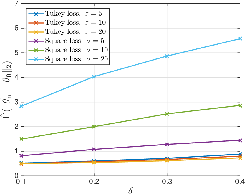
Figure 8: Robust regression: (a)(a) The standard deviation of each iteration point with respect to random initialization, for different proportion of contamination. (b)(b) The robustness of the global minimum between linear regression and Tukey regression.

In Figures 8(a), 8(b) we study the a contaminated model for the noise, namely εi∼(1−δ)​𝖭​(0,1)+δ​𝖭​(0,σ2)\varepsilon_{i}\sim(1-\delta){\sf N}(0,1)+\delta{\sf N}(0,\sigma^{2}). In Figure 8(a) we plot the standard deviation of the estimates obtained with random initializations 𝜽s∼𝖭⁡(𝟎,25​Id×d/d){\bm{\theta}}_{s}\sim{\sf N}({\bm{0}},25\,{\rm I}_{d\times d}/d), for n=480n=480, d=80d=80. Convergence rate remains exponential even for large contamination fraction. In Figure 8(b) we investigated the dependence of the estimation error on the contamination fraction, and the scale of outliers. Tukey’s regression is fairly insensitive to outliers, while the least squares regression deteriorates as expected.

5.4 Gaussian mixture model

Refer to caption
(a)
Refer to caption
(b)
Figure 9: Gaussian mixture model: (a)(a) The convergence of statistical error. Here we use ‖𝜽0,1−𝜽0,2‖2=3\|{\bm{\theta}}_{0,1}-{\bm{\theta}}_{0,2}\|_{2}=3, and n/d=6n/d=6; (b)(b) The convergence of the gradient descent algorithm.

In Figures 9(a) and 9(b) we consider the Gaussian mixture model of Section 4.5. We use an equal mixture proportion with ‖𝜽0,1−𝜽0,2‖2=3\|{\bm{\theta}}_{0,1}-{\bm{\theta}}_{0,2}\|_{2}=3 and compute the maximum likelihood estimator (30). Instead of using trust region method as suggested in Theorem 8, we used gradient descent here. We observed that there are only two local minimizers. In Figure 9(a) we plot the convergence of the statistical error, and in Figure 9(b) the convergence of the gradient descent algorithm to one of the only two local minimizers. These results are consistent with Theorem 8.

5.5 Australian credit data

Refer to caption
Figure 10: Australian credit data: the standard deviation of each iteration point with respect to random initialization.

In Figure 10 we consider the Australian credit dataset from Statlog [Lic13]. The data set contains n=690n=690 entries. Each entries has a binary label, with 307307 entries labeled 11 and 383383 labeled 00. Each entry also comprises d=14d=14 attributes including both categorical and continuous variables. These variables are normalized with zero mean and unit standard deviation.

We fit a model of the form ℙ⁡(Yi=1|𝑿i=𝒙)=σ⁡(⟨𝜽0,𝒙⟩)\mathbb{P}(Y_{i}=1|{\bm{X}}_{i}={\bm{x}})=\sigma(\langle{\bm{\theta}}_{0},{\bm{x}}\rangle) with σ​(u)=σL​(u)\sigma(u)=\sigma_{L}(u) the logistic function, by using the non-convex approach (23) and gradient descent. We also used logistic regression for comparison. Let us emphasize here that our focus here is not on the accuracy of the predictive model, but rather on showing that the non-convex approach is a viable alternative to the standard logistic regression. In particular, the M-estimator appears to be efficiently computable.

In Figure 10, we plot the standard deviation of the estimate 𝜽^n​(i)\hat{\bm{\theta}}_{n}(i), over random initializations 𝜽s∼𝖭⁡(𝟎,Id×d/d){\bm{\theta}}_{s}\sim{\sf N}({\bm{0}},{\rm I}_{d\times d}/d). As for the simulations in the previous section, the standard deviation decreases exponentially fast, suggesting that indeed the optimization problem has a unique local minimum.

5.6 Colon cancer data

Refer to caption
(a)
Refer to caption
(b)
Figure 11: Colon cancer data: (a)(a) The standard deviation of each iteration point with respect to random initialization, for different regularization parameter. (b)(b) Number of non-zero elements of logistic Lasso and non-convex logistic Lasso.

In Figures 11(a), 11(b) we consider a gene-expression dataset from [ABN+99]. The data set contains expression levels of of 2,0002,000 genes in 2222 normal and 4040 tumor colon tissues, hence n=62n=62 data points. Expression levels are normalized as in [ABN+99] to have zero mean and unit standard deviation. We use the expression levels to form feature vectors 𝒙i∈ℝd{\bm{x}}_{i}\in{\mathbb{R}}^{d}, d=2000d=2000 and encode the type of tissue using a binary label yi=1y_{i}=1 (tumor) or yi=0y_{i}=0 (no tissue).

We fit a model of the form ℙ⁡(Yi=1|𝑿i=𝒙)=σ⁡(⟨𝜽0,𝒙⟩){\mathbb{P}}(Y_{i}=1|{\bm{X}}_{i}={\bm{x}})=\sigma(\langle{\bm{\theta}}_{0},{\bm{x}}\rangle) with σ​(u)=σL​(u)\sigma(u)=\sigma_{L}(u) the logistic function, by using the non-convex approach (25) and proximal gradient. We also used ℓ1\ell_{1}-regularized logistic regression, for comparison. Let us emphasize here that our focus here is not on the accuracy of the predictive model, but rather on showing that the non-convex approach is a viable alternative to the more standard regularized logistic regression.

In Figure 11(a), we plot the standard deviation of the estimate 𝜽^n​(i)\hat{\bm{\theta}}_{n}(i), over random initializations 𝜽s∼𝖭⁡(𝟎,Id×d/d){\bm{\theta}}_{s}\sim{\sf N}({\bm{0}},{\rm I}_{d\times d}/d). As for the simulations in the previous section, the standard deviation decreases exponentially fast, suggesting that indeed the optimization problem has a unique local minimum. In Figure 11(b) we compare the model selected by the non-convex approach (25) to the one from ℓ1\ell_{1}-regularized logistic regression, and also plot the number of overlaps of their selected variables. Note that most of the covariates selected by the non-convex regression method also appear in logistic regression. This suggests that the model produced by the non-convex approach is comparable to that produced by ℓ1\ell_{1}-regularized logistic regression.

Acknowledgments

A.M. was partially supported by the NSF grant CCF-1319979. S.M. was supported by Office of Technology Licensing Stanford Graduate Fellowship.

Appendix A Some useful tools

In this section we collect some well-known definitions and tools from high-dimensional probability, for the reader’s convenience.

A.1 Properties of sub-Gaussian and sub-exponential random variables

Let us first recall the definition of (not necessarily mean zero) sub-Gaussian and sub-exponential random variables in ℝd\mathbb{R}^{d}:

Definition 2.

A random variable 𝑿∈ℝd{\bm{X}}\in\mathbb{R}^{d} is τ2\tau^{2}-sub-Gaussian if for any 𝝀∈ℝd{\bm{\lambda}}\in\mathbb{R}^{d},

𝔼⁡[e⟨𝝀,𝑿−𝔼⁡[𝑿]⟩]≤e‖𝝀‖22​τ22.{\mathbb{E}}[e^{\langle{\bm{\lambda}},{\bm{X}}-{\mathbb{E}}[{\bm{X}}]\rangle}]\leq e^{\frac{\|{\bm{\lambda}}\|_{2}^{2}\tau^{2}}{2}}. (34)
Definition 3.

A random variable 𝑿∈ℝd{\bm{X}}\in\mathbb{R}^{d} is KK-sub-exponential if for any 𝝀∈ℝd{\bm{\lambda}}\in\mathbb{R}^{d}, ‖⟨𝝀,𝑿−𝔼⁡[𝑿]⟩‖ψ1≤K​‖𝝀‖2\|\langle{\bm{\lambda}},{\bm{X}}-{\mathbb{E}}[{\bm{X}}]\rangle\|_{\psi_{1}}\leq K\|{\bm{\lambda}}\|_{2}, where ∥⋅∥ψ1\|\cdot\|_{\psi_{1}} is the Orlicz ψ1\psi_{1}-norm:

‖X‖ψ1:=supk≥11k​𝔼​[|X−𝔼⁡(X)|k]1/k.\|X\|_{\psi_{1}}\mathrel{\mathop{:}}=\sup_{k\geq 1}\frac{1}{k}{\mathbb{E}}[|X-{\mathbb{E}}(X)|^{k}]^{1/k}. (35)

Note: we can also define sub-Gaussian random variables via the Orlicz ψ2\psi_{2}-norm. We choose to follow the more classic definition there so as to make sub-Gaussian concentration inequalities clearer.

Proofs of our main theorems rely on some properties about sub-Gaussian and sub-exponential random variables that are well known in the literature, for example [BLM13, Ver12]. We summarize them here for reference.

Lemma 1.

Assume 𝐗∈ℝd{\bm{X}}\in\mathbb{R}^{d} has mean zero and is τ2\tau^{2}-sub-Gaussian, then

  1. (a)(a)

    There exists numerical constants C2​k∈(0,∞)C_{2k}\in(0,\infty) for all integers k≥1k\geq 1 such that

    𝔼⁡[|⟨𝒖,𝑿⟩|2​k]≤C2​k​‖𝒖‖22​k​τ2​k{\mathbb{E}}[|\langle{\bm{u}},{\bm{X}}\rangle|^{2k}]\leq C_{2k}\|{\bm{u}}\|_{2}^{2k}\tau^{2k} (36)

    for all 𝒖∈ℝd{\bm{u}}\in\mathbb{R}^{d}. In particular, C2=1C_{2}=1, and we can take C2​k=2k+1​k!C_{2k}=2^{k+1}k!.

  2. (b)(b)

    Higher moments of ‖𝑿‖2\|{\bm{X}}\|_{2} are controlled, that is, for all integers k≥1k\geq 1,

    𝔼⁡[‖𝑿‖22​k]≤C2​k​dk​τ2​k,{\mathbb{E}}[\|{\bm{X}}\|_{2}^{2k}]\leq C_{2k}d^{k}\tau^{2k}, (37)

    where C2​kC_{2k} is the same as in (a)(a).

  3. (c)(c)

    ‖𝑿‖22\|{\bm{X}}\|_{2}^{2} is 4​τ24\tau^{2}-sub-exponential. In particular

    𝔼⁡[e‖𝑿‖224​τ2]≤2d2<ed2.{\mathbb{E}}[e^{\frac{\|{\bm{X}}\|_{2}^{2}}{4\tau^{2}}}]\leq 2^{\frac{d}{2}}<e^{\frac{d}{2}}. (38)
  4. (d)(d)

    If X∈ℝX\in\mathbb{R} is zero-mean and τ2\tau^{2}-sub-Gaussian and α\alpha is a random variable (that can depend on XX) with |α|≤1|\alpha|\leq 1, then there exists some absolute constant Cs​g≤64C_{sg}\leq 64 such that α​X\alpha X is Cs​g​τ2C_{sg}\tau^{2}-sub-Gaussian.

  5. (e)(e)

    If X∈ℝX\in\mathbb{R} is zero-mean KK-sub-exponential and β\beta is a random variable (that can depend on XX) with |β|≤1|\beta|\leq 1, then there exists some absolute constant Cs​e≤2C_{se}\leq 2 such that β​X\beta X is Cs​e​KC_{se}K-sub-exponential.

  6. (f)(f)
    𝔼⁡[‖𝑿‖∞]≤2​τ2​log⁡(2​d).{\mathbb{E}}[\|{\bm{X}}\|_{\infty}]\leq\sqrt{2\tau^{2}\log(2d)}. (39)
Proof.
  1. (a)(a)

    This is known in the literature, for example Theorem 2.1 in [BLM13].

  2. (b)(b)

    This is a direct consequence of part (a)(a). From the generalized mean inequality, we have

    𝔼⁡[‖𝑿‖22​k]=𝔼⁡[(∑j=1dXj2)k]≤dk−1​𝔼​[∑j=1dXj2​k].{\mathbb{E}}[\|{\bm{X}}\|_{2}^{2k}]={\mathbb{E}}\Big[(\sum_{j=1}^{d}X_{j}^{2})^{k}\Big]\leq d^{k-1}{\mathbb{E}}\Big[\sum_{j=1}^{d}X_{j}^{2k}\Big]. (40)

    Applying part (a)(a) with the standard basis 𝒆j∈ℝd{\bm{e}}_{j}\in\mathbb{R}^{d}, we get 𝔼⁡[Xj2​k]≤C2​k​τ2​k{\mathbb{E}}[X_{j}^{2k}]\leq C_{2k}\tau^{2k}. Summing over jj gives 𝔼⁡[‖𝑿‖22​k]≤dk​C2​k​τ2​k{\mathbb{E}}[\|{\bm{X}}\|_{2}^{2k}]\leq d^{k}C_{2k}\tau^{2k}.

  3. (c)(c)

    We can assume τ2=1\tau^{2}=1 by scale invariance. Let 𝑾∼𝖭⁡(0,Id×d){\bm{W}}\sim{\sf N}(0,{\rm I}_{d\times d}) be independent of 𝑿{\bm{X}}. It is known that 𝔼⁡[eλ​Z2]=11−2​λ{\mathbb{E}}[e^{\lambda Z^{2}}]=\frac{1}{\sqrt{1-2\lambda}} for Z∼𝖭⁡(0,1)Z\sim{\sf N}(0,1) and λ<12\lambda<\frac{1}{2}, so we have

    𝔼⁡[eλ​‖𝑾‖22]=∏i=1d𝔼⁡[eλ​Wi2]=1(1−2​λ)d/2{\mathbb{E}}[e^{\lambda\|{\bm{W}}\|_{2}^{2}}]=\prod_{i=1}^{d}{\mathbb{E}}[e^{\lambda W_{i}^{2}}]=\frac{1}{(1-2\lambda)^{d/2}} (41)

    for any λ<12\lambda<\frac{1}{2}.

    Now, for λ>0\lambda>0, we evaluate the quantity 𝔼⁡[e2​λ​⟨𝑿,𝑾⟩]{\mathbb{E}}[e^{\sqrt{2\lambda}\langle{\bm{X}},{\bm{W}}\rangle}] in two ways. We have

    𝔼⁡[e2​λ​⟨𝑿,𝑾⟩]=𝔼⁡[𝔼⁡[e2​λ​⟨𝑿,𝑾⟩|𝑿]]=𝔼⁡[e‖2​λ​𝑿‖222]=𝔼⁡[eλ​‖𝑿‖22].{\mathbb{E}}[e^{\sqrt{2\lambda}\langle{\bm{X}},{\bm{W}}\rangle}]={\mathbb{E}}\Big[{\mathbb{E}}[e^{\sqrt{2\lambda}\langle{\bm{X}},{\bm{W}}\rangle}|{\bm{X}}]\Big]={\mathbb{E}}\Big[e^{\frac{\|\sqrt{2\lambda}{\bm{X}}\|_{2}^{2}}{2}}\Big]={\mathbb{E}}[e^{\lambda\|{\bm{X}}\|_{2}^{2}}]. (42)

    On the other hand, we have

    𝔼⁡[e2​λ​⟨𝑿,𝑾⟩]=𝔼⁡[𝔼⁡[e⟨2​λ​𝑾,𝑿⟩|𝑾]]≤𝔼⁡[e‖2​λ​𝑾‖222]=𝔼⁡[eλ​‖𝑾‖22]=1(1−2​λ)d/2,{\mathbb{E}}[e^{\sqrt{2\lambda}\langle{\bm{X}},{\bm{W}}\rangle}]={\mathbb{E}}\Big[{\mathbb{E}}[e^{\langle\sqrt{2\lambda}{\bm{W}},{\bm{X}}\rangle}|{\bm{W}}]\Big]\leq{\mathbb{E}}[e^{\frac{\|\sqrt{2\lambda}{\bm{W}}\|_{2}^{2}}{2}}]={\mathbb{E}}[e^{\lambda\|{\bm{W}}\|_{2}^{2}}]=\frac{1}{(1-2\lambda)^{d/2}}, (43)

    the last equality holding for λ<12\lambda<\frac{1}{2}. Combining (42) and (43) and taking λ=14\lambda=\frac{1}{4}, we get

    𝔼⁡[e‖𝑿‖224]≤2d/2<ed/2.{\mathbb{E}}[e^{\frac{\|{\bm{X}}\|_{2}^{2}}{4}}]\leq 2^{d/2}<e^{d/2}. (44)
  4. (d)(d)

    By Theorem 2.1 in [BLM13], we have 𝔼⁡[|X|2​k]≤k!​(4​τ2)k{\mathbb{E}}[|X|^{2k}]\leq k!(4\tau^{2})^{k}. Consequently, 𝔼⁡[|α​X|2​k]≤k!​(4​τ2)k{\mathbb{E}}[|\alpha X|^{2k}]\leq k!(4\tau^{2})^{k}, since |α|≤1|\alpha|\leq 1. Now we introduce (α′,X′)(\alpha^{\prime},X^{\prime}) that is an independent copy of (α,X)(\alpha,X), then

    𝔼⁡[|α​X−α′​X′|2​k]≤22​k−1​𝔼​[|α​X|2​k+|α′​X′|2​k]=22​k​𝔼​[|α​X|2​k]≤k!​(16​τ2)k.{\mathbb{E}}[|\alpha X-\alpha^{\prime}X^{\prime}|^{2k}]\leq 2^{2k-1}{\mathbb{E}}[|\alpha X|^{2k}+|\alpha^{\prime}X^{\prime}|^{2k}]=2^{2k}{\mathbb{E}}[|\alpha X|^{2k}]\leq k!(16\tau^{2})^{k}. (45)

    We apply the converse statement in [BLM13, Theorem 2.1], to conclude that α​X−α′​X′\alpha X-\alpha^{\prime}X^{\prime} is 64​τ264\tau^{2}-sub-Gaussian. Finally, as eλ⁡(a−t)e^{\lambda(a-t)} is convex in tt, we have

    𝔼⁡[eλ⁡(α​X−𝔼⁡[α​X])]=𝔼⁡[eλ⁡(α​X−𝔼⁡[α′​X′])]≤𝔼⁡[eλ⁡(α​X−α′​X′)],{\mathbb{E}}[e^{\lambda(\alpha X-{\mathbb{E}}[\alpha X])}]={\mathbb{E}}[e^{\lambda(\alpha X-{\mathbb{E}}[\alpha^{\prime}X^{\prime}])}]\leq{\mathbb{E}}[e^{\lambda(\alpha X-\alpha^{\prime}X^{\prime})}], (46)

    and thus α​X\alpha X is also 64​τ264\tau^{2}-sub-Gaussian.

  5. (e)(e)

    By Remark 5.18 in [Ver12], we have

    ‖β​X−𝔼⁡[β​X]‖ψ1≤2​‖β​X‖ψ1≤2​‖X‖ψ1.\|\beta X-{\mathbb{E}}[\beta X]\|_{\psi_{1}}\leq 2\|\beta X\|_{\psi_{1}}\leq 2\|X\|_{\psi_{1}}\,. (47)
  6. (f)(f)

    It suffices to work with τ=1\tau=1. For any λ>0\lambda>0, we have

    𝔼⁡[eλ​‖𝑿‖∞]=𝔼⁡[eλ​maxj∈[d]​{Xj,−Xj}]≤∑j=1d𝔼⁡[eλ​Xj]+∑j=1d𝔼⁡[e−λ​Xj]≤2​d​eλ22.{\mathbb{E}}[e^{\lambda\|{\bm{X}}\|_{\infty}}]={\mathbb{E}}[e^{\lambda\max_{j\in[d]}\{X_{j},-X_{j}\}}]\leq\sum_{j=1}^{d}{\mathbb{E}}[e^{\lambda X_{j}}]+\sum_{j=1}^{d}{\mathbb{E}}[e^{-\lambda X_{j}}]\leq 2de^{\frac{\lambda^{2}}{2}}.

    Applying Jensen’s inequality on the function t↦eλ​tt\mapsto e^{\lambda t}, we get

    𝔼⁡[‖X‖∞]≤1λ​log⁡𝔼⁡[eλ​‖𝑿‖∞]≤1λ​(λ22+log⁡(2​d)).{\mathbb{E}}[\|X\|_{\infty}]\leq\frac{1}{\lambda}\log{\mathbb{E}}[e^{\lambda\|{\bm{X}}\|_{\infty}}]\leq\frac{1}{\lambda}\Big(\frac{\lambda^{2}}{2}+\log(2d)\Big).

    Optimizing the RHS gives λ∗=2​log⁡(2​d)\lambda^{*}=\sqrt{2\log(2d)} and an upper bound 2​log⁡(2​d)\sqrt{2\log(2d)}.

∎

Lemma 2.

There exists a universal constant CsC_{s}, such that the sum of two dependent sub-Gaussian random variables with parameters τ12\tau_{1}^{2} and τ22\tau_{2}^{2} is Cs​(τ12+τ22)C_{s}(\tau_{1}^{2}+\tau_{2}^{2})-sub-Gaussian, and the sum of two dependent sub-exponential random variables with parameters τ12\tau_{1}^{2} and τ22\tau_{2}^{2} is Cs​(τ12+τ22)C_{s}(\tau_{1}^{2}+\tau_{2}^{2})-sub-exponential.

Proof.

This lemma follows directly from the equivalent form of definition of sub-Gaussian and sub-exponential random variables using Orlicz norms. ∎

Theorem 9 (Bernstein inequality for subexponential random variables).

Let X1,…​XnX_{1},\dots X_{n} be independent sub-exponential random variables with ‖Xi‖ψ1≤b\|X_{i}\|_{\psi_{1}}\leq b, and define Sn≡∑i=1n(Xi−𝔼​Xi)S_{n}\equiv\sum_{i=1}^{n}\big(X_{i}-{\mathbb{E}}X_{i}\big). Then there exists a universal constant cc such that, for all t>0t>0,

ℙ⁡(Sn≥t)≤exp⁡{−c​min⁡(t2n​b2,tb)}.\displaystyle{\mathbb{P}}\big(S_{n}\geq t\big)\leq\exp\Big\{-c\min\Big(\frac{t^{2}}{nb^{2}},\frac{t}{b}\Big)\Big\}\,. (48)

A.2 Bounding norms via ε\varepsilon-covers

In this section we state two simple technical lemmas that are useful for our proofs. Their proofs of these lemmas can be found in [Ver12].

Lemma 3.

Let a∈ℝda\in\mathbb{R}^{d} and Vε={𝐯1,…,𝐯N}V_{\varepsilon}=\{{\bm{v}}_{1},\dots,{\bm{v}}_{N}\} be an ε\varepsilon-cover of 𝖡d​(𝟎,1){\sf B}^{d}({\bm{0}},1), then

‖𝒂‖2≤11−ε​sup𝒗∈Vε⟨𝒗,𝒂⟩.\|{\bm{a}}\|_{2}\leq\frac{1}{1-\varepsilon}\sup_{{\bm{v}}\in V_{\varepsilon}}\langle{\bm{v}},{\bm{a}}\rangle. (49)
Lemma 4.

Let 𝐌∈ℝd×d{\bm{M}}\in\mathbb{R}^{d\times d} be a symmetric d×dd\times d matrix and Vε={𝐯1,…,𝐯N}V_{\varepsilon}=\{{\bm{v}}_{1},\dots,{\bm{v}}_{N}\} be an ε\varepsilon-cover of 𝖡d​(𝟎,1){\sf B}^{d}({\bm{0}},1), then

‖𝑴‖op≤11−2​ε​sup𝒗∈Vε|⟨𝒗,𝑴​𝒗⟩|.\|{\bm{M}}\|_{\rm op}\leq\frac{1}{1-2\varepsilon}\sup_{{\bm{v}}\in V_{\varepsilon}}|\langle{\bm{v}},{\bm{M}}{\bm{v}}\rangle|. (50)

Appendix B Proof of Theorem 1: High-dimensional regime

B.1 Proof of Theorem 1.(a)(a): Uniform convergence of gradient

Step 1. Decompose the bad events using ε\varepsilon-nets.

Let NεN_{\varepsilon} be the ε\varepsilon-covering number of the ball 𝖡p​(𝟎,r){\sf B}^{p}({\bm{0}},r). It is known that log⁡Nε≤p​log⁡(3​r/ε)\log N_{\varepsilon}\leq p\log(3r/\varepsilon) [Ver12]. Let Θε={𝜽1,…,𝜽N}\Theta_{\varepsilon}=\{{\bm{\theta}}_{1},\ldots,{\bm{\theta}}_{N}\} be a corresponding ε\varepsilon-cover with N=NεN=N_{\varepsilon} elements. For any 𝜽∈𝖡p​(𝟎,r){\bm{\theta}}\in{\sf B}^{p}({\bm{0}},r), let j⁡(𝜽)=arg​minj∈[N]⁡‖𝜽−𝜽j‖2j({\bm{\theta}})=\argmin_{j\in[N]}\|{\bm{\theta}}-{\bm{\theta}}_{j}\|_{2}. Then ‖𝜽−𝜽j⁡(𝜽)‖2≤ε\|{\bm{\theta}}-{\bm{\theta}}_{j({\bm{\theta}})}\|_{2}\leq\varepsilon for all 𝜽∈𝖡p​(𝟎,r){\bm{\theta}}\in{\sf B}^{p}({\bm{0}},r).

Observe that ∇R^n​(𝜽)=1n​∑i=1n∇ℓ​(𝜽,𝒁i)\nabla\widehat{R}_{n}({\bm{\theta}})=\frac{1}{n}\sum_{i=1}^{n}\nabla\ell({\bm{\theta}};{\bm{Z}}_{i}), and ∇R​(𝜽)=𝔼⁡[∇ℓ​(𝜽,𝒁)]\nabla R({\bm{\theta}})={\mathbb{E}}[\nabla\ell({\bm{\theta}};{\bm{Z}})]. Thus, for any 𝜽∈𝖡p​(𝟎,r){\bm{\theta}}\in{\sf B}^{p}({\bm{0}},r), we have

‖∇R^n​(𝜽)−∇R​(𝜽)‖2≤\displaystyle\Big\|\nabla\widehat{R}_{n}({\bm{\theta}})-\nabla R({\bm{\theta}})\Big\|_{2}\leq ‖1n​∑i=1n[∇ℓ​(𝜽,𝒁i)−∇ℓ​(𝜽j⁡(𝜽),𝒁i)]‖2\displaystyle\Big\|\frac{1}{n}\sum_{i=1}^{n}\Big[\nabla\ell({\bm{\theta}};{\bm{Z}}_{i})-\nabla\ell({\bm{\theta}}_{j({\bm{\theta}})};{\bm{Z}}_{i})\Big]\Big\|_{2} (51)
+‖1n​∑i=1n∇ℓ​(𝜽j⁡(𝜽),𝒁i)−𝔼⁡[∇ℓ​(𝜽j⁡(𝜽),𝒁)]‖2\displaystyle+\Big\|\frac{1}{n}\sum_{i=1}^{n}\nabla\ell({\bm{\theta}}_{j({\bm{\theta}})};{\bm{Z}}_{i})-{\mathbb{E}}[\nabla\ell({\bm{\theta}}_{j({\bm{\theta}})};{\bm{Z}})]\Big\|_{2}
+‖𝔼⁡[∇ℓ​(𝜽j⁡(𝜽),𝒁)]−𝔼⁡[∇ℓ​(𝜽,𝒁)]‖2.\displaystyle+\Big\|{\mathbb{E}}[\nabla\ell({\bm{\theta}}_{j({\bm{\theta}})};{\bm{Z}})]-{\mathbb{E}}[\nabla\ell({\bm{\theta}};{\bm{Z}})]\Big\|_{2}.

Hence, we have

ℙ⁡(sup𝜽∈𝖡p​(𝟎,r)‖∇R^n​(𝜽)−∇R​(𝜽)‖2≥t)≤ℙ⁡(At)+ℙ⁡(Bt)+ℙ⁡(Ct),\mathbb{P}\left(\sup_{{\bm{\theta}}\in{\sf B}^{p}({\bm{0}},r)}\left\|\nabla\widehat{R}_{n}({\bm{\theta}})-\nabla R({\bm{\theta}})\right\|_{2}\geq t\right)\leq\mathbb{P}(A_{t})+\mathbb{P}(B_{t})+\mathbb{P}(C_{t}),

where the events AtA_{t}, BtB_{t}, and CtC_{t} are defined as

At=\displaystyle A_{t}= {sup𝜽∈𝖡p​(𝟎,r)‖1n∑i=1n[∇ℓ(𝜽;𝒁i)−∇ℓ(𝜽j⁡(𝜽);𝒁i)]‖2≥t3},\displaystyle\left\{\sup_{{\bm{\theta}}\in{\sf B}^{p}({\bm{0}},r)}\left\|\frac{1}{n}\sum_{i=1}^{n}\Big[\nabla\ell({\bm{\theta}};{\bm{Z}}_{i})-\nabla\ell({\bm{\theta}}_{j({\bm{\theta}})};{\bm{Z}}_{i})\Big]\right\|_{2}\geq\frac{t}{3}\right\},
Bt=\displaystyle B_{t}= {supj∈[N]‖1n∑i=1n∇ℓ(𝜽j;𝒁i)−𝔼[∇ℓ(𝜽j;𝒁)]‖2≥t3},\displaystyle\left\{\sup_{j\in[N]}\left\|\frac{1}{n}\sum_{i=1}^{n}\nabla\ell({\bm{\theta}}_{j};{\bm{Z}}_{i})-{\mathbb{E}}[\nabla\ell({\bm{\theta}}_{j};{\bm{Z}})]\right\|_{2}\geq\frac{t}{3}\right\},
Ct=\displaystyle C_{t}= {sup𝜽∈𝖡p​(𝟎,r)∥𝔼[∇ℓ(𝜽j⁡(𝜽);𝒁)]−𝔼[∇ℓ(𝜽;𝒁)]∥2≥t3}.\displaystyle\left\{\sup_{{\bm{\theta}}\in{\sf B}^{p}({\bm{0}},r)}\Big\|{\mathbb{E}}[\nabla\ell({\bm{\theta}}_{j({\bm{\theta}})};{\bm{Z}})]-{\mathbb{E}}[\nabla\ell({\bm{\theta}};{\bm{Z}})]\Big\|_{2}\geq\frac{t}{3}\right\}.

Step 2. Upper bound ℙ⁡(Bt)\mathbb{P}(B_{t}).

Let V1/2V_{1/2} be a (1/2)(1/2)-cover of 𝖡p​(𝟎,1){\sf B}^{p}({\bm{0}},1) with log⁡|V1/2|≤p​log⁡6\log|V_{1/2}|\leq p\log 6. From Lemma 3 we know that

‖1n​∑i=1n∇ℓ​(𝜽j,𝒁i)−𝔼⁡[∇ℓ​(𝜽j,𝒁)]‖2≤2​sup𝒗∈V1/2⟨𝒗,1n​∑i=1n∇ℓ​(𝜽j,𝒁i)−𝔼⁡[∇ℓ​(𝜽j,𝒁)]⟩.\left\|\frac{1}{n}\sum_{i=1}^{n}\nabla\ell({\bm{\theta}}_{j};{\bm{Z}}_{i})-{\mathbb{E}}[\nabla\ell({\bm{\theta}}_{j};{\bm{Z}})]\right\|_{2}\leq 2\sup_{{\bm{v}}\in V_{1/2}}\Big\langle{\bm{v}},\frac{1}{n}\sum_{i=1}^{n}\nabla\ell({\bm{\theta}}_{j};{\bm{Z}}_{i})-{\mathbb{E}}[\nabla\ell({\bm{\theta}}_{j};{\bm{Z}})]\Big\rangle.

Taking union bounds over Θε\Theta_{\varepsilon} and V1/2V_{1/2} yields

ℙ⁡(Bt)≤\displaystyle\mathbb{P}(B_{t})\leq ℙ⁡(supj∈[N],𝒗∈V1/2{1n​∑i=1n⟨∇ℓ​(𝜽j,𝒁i)−𝔼⁡[∇ℓ​(𝜽j,𝒁)],𝒗⟩}≥t6)\displaystyle\mathbb{P}\left(\sup_{j\in[N],{\bm{v}}\in V_{1/2}}\left\{\frac{1}{n}\sum_{i=1}^{n}\Big\langle\nabla\ell({\bm{\theta}}_{j};{\bm{Z}}_{i})-{\mathbb{E}}[\nabla\ell({\bm{\theta}}_{j};{\bm{Z}})],{\bm{v}}\Big\rangle\right\}\geq\frac{t}{6}\right)
≤\displaystyle\leq ep​log⁡3​rε+p​log⁡6​supj∈[N],𝒗∈V1/2ℙ⁡(1n​∑i=1n⟨∇ℓ​(𝜽j,𝒁i)−𝔼⁡[∇ℓ​(𝜽j,𝒁)],𝒗⟩≥t6).\displaystyle e^{p\log\frac{3r}{\varepsilon}+p\log 6}\sup_{j\in[N],{\bm{v}}\in V_{1/2}}\mathbb{P}\left(\frac{1}{n}\sum_{i=1}^{n}\Big\langle\nabla\ell({\bm{\theta}}_{j};{\bm{Z}}_{i})-{\mathbb{E}}[\nabla\ell({\bm{\theta}}_{j};{\bm{Z}})],{\bm{v}}\Big\rangle\geq\frac{t}{6}\right).

Fixing any jj and 𝒗{\bm{v}}, according to Assumption 1, we have ⟨∇ℓ​(𝜽j,𝒁i)−𝔼⁡[∇ℓ​(𝜽j,𝒁)],𝒗⟩\langle\nabla\ell({\bm{\theta}}_{j};{\bm{Z}}_{i})-{\mathbb{E}}[\nabla\ell({\bm{\theta}}_{j};{\bm{Z}})],{\bm{v}}\rangle is τ2\tau^{2}-sub-Gaussian. Hence 1n​∑i=1n⟨∇ℓ​(𝜽j,𝒁i)−𝔼⁡[∇ℓ​(𝜽j,𝒁)],𝒗⟩\frac{1}{n}\sum_{i=1}^{n}\Big\langle\nabla\ell({\bm{\theta}}_{j};{\bm{Z}}_{i})-{\mathbb{E}}[\nabla\ell({\bm{\theta}}_{j};{\bm{Z}})],{\bm{v}}\Big\rangle is τ2/n\tau^{2}/n-sub-Gaussian random variable. This gives

ℙ⁡(1n​∑i=1n⟨∇ℓ​(𝜽j,𝒁i)−𝔼⁡[∇ℓ​(𝜽j,𝒁)],𝒗⟩≥t6)≤e−n​t2144​τ2.\mathbb{P}\left(\frac{1}{n}\sum_{i=1}^{n}\Big\langle\nabla\ell({\bm{\theta}}_{j};{\bm{Z}}_{i})-{\mathbb{E}}[\nabla\ell({\bm{\theta}}_{j};{\bm{Z}})],{\bm{v}}\Big\rangle\geq\frac{t}{6}\right)\leq e^{-\frac{nt^{2}}{144\tau^{2}}}.

As a result,

ℙ⁡(Bt)≤exp⁡(−n​t2144​τ2+p​log⁡18​rε).\mathbb{P}(B_{t})\leq\exp\left(-\frac{nt^{2}}{144\tau^{2}}+p\log\frac{18r}{\varepsilon}\right).

Thus,

t>144​τ2​(p​log⁡18​rε+log⁡2δ)nt>\sqrt{\frac{144\tau^{2}(p\log\frac{18r}{\varepsilon}+\log\frac{2}{\delta})}{n}}

ensures that ℙ⁡(Bt)≤δ/2\mathbb{P}(B_{t})\leq\delta/2.

Step 3. Upper bound ℙ⁡(At)\mathbb{P}(A_{t}) and ℙ⁡(Ct)\mathbb{P}(C_{t}).

Let us look at the deterministic event CtC_{t} first. We have

sup𝜽∈𝖡p​(𝟎,r)‖𝔼⁡[∇ℓ​(𝜽,𝒁)−∇ℓ​(𝜽j⁡(𝜽),𝒁)]‖2\displaystyle\sup_{{\bm{\theta}}\in{\sf B}^{p}({\bm{0}},r)}\left\|{\mathbb{E}}[\nabla\ell({\bm{\theta}};{\bm{Z}})-\nabla\ell({\bm{\theta}}_{j({\bm{\theta}})};{\bm{Z}})]\right\|_{2}
≤\displaystyle\leq sup𝜽∈𝖡p​(𝟎,r)‖𝔼⁡[∇ℓ​(𝜽,𝒁)−∇ℓ​(𝜽j⁡(𝜽),𝒁)]‖2‖𝜽−𝜽j⁡(𝜽)‖2⋅sup𝜽∈𝖡p​(𝟎,r)‖𝜽−𝜽j⁡(𝜽)‖2\displaystyle\sup_{{\bm{\theta}}\in{\sf B}^{p}({\bm{0}},r)}\frac{\left\|{\mathbb{E}}[\nabla\ell({\bm{\theta}};{\bm{Z}})-\nabla\ell({\bm{\theta}}_{j({\bm{\theta}})};{\bm{Z}})]\right\|_{2}}{\|{\bm{\theta}}-{\bm{\theta}}_{j({\bm{\theta}})}\|_{2}}\cdot\sup_{{\bm{\theta}}\in{\sf B}^{p}({\bm{0}},r)}\|{\bm{\theta}}-{\bm{\theta}}_{j({\bm{\theta}})}\|_{2}
≤\displaystyle\leq 𝔼⁡[sup𝜽∈𝖡p​(𝟎,r)‖∇2R^​(𝜽)‖op]⋅ε\displaystyle{\displaystyle\mathbb{E}}\left[\sup_{{\bm{\theta}}\in{\sf B}^{p}({\bm{0}},r)}\|\nabla^{2}\widehat{R}({\bm{\theta}})\|_{{\rm op}}\right]\cdot\varepsilon
≤\displaystyle\leq D∗⋅ε,\displaystyle D_{*}\cdot\varepsilon,

where

D∗=\displaystyle D_{*}= 𝔼⁡[sup𝜽∈𝖡p​(𝟎,r)‖∇2R^​(𝜽)‖op]\displaystyle{\displaystyle\mathbb{E}}\left[\sup_{{\bm{\theta}}\in{\sf B}^{p}({\bm{0}},r)}\|\nabla^{2}\widehat{R}({\bm{\theta}})\|_{{\rm op}}\right]
≤\displaystyle\leq 𝔼⁡[sup𝜽∈𝖡p​(𝟎,r)‖∇2R^​(𝜽)−∇2R​(𝜽∗)‖op]+‖∇2R​(𝜽∗)‖op\displaystyle{\displaystyle\mathbb{E}}\left[\sup_{{\bm{\theta}}\in{\sf B}^{p}({\bm{0}},r)}\|\nabla^{2}\widehat{R}({\bm{\theta}})-\nabla^{2}R({\bm{\theta}}_{*})\|_{{\rm op}}\right]+\|\nabla^{2}R({\bm{\theta}}_{*})\|_{\rm op}
≤\displaystyle\leq 𝔼⁡[sup𝜽∈𝖡p​(𝟎,r)‖1n​∑i=1n∇2ℓ​(𝜽,𝒁i)−𝔼⁡[∇2ℓ​(𝜽∗,𝒁)]‖op]+H\displaystyle{\displaystyle\mathbb{E}}\left[\sup_{{\bm{\theta}}\in{\sf B}^{p}({\bm{0}},r)}\left\|\frac{1}{n}\sum_{i=1}^{n}\nabla^{2}\ell({\bm{\theta}};{\bm{Z}}_{i})-{\mathbb{E}}[\nabla^{2}\ell({\bm{\theta}}_{*};{\bm{Z}})]\right\|_{{\rm op}}\right]+H
≤\displaystyle\leq 𝔼⁡[sup𝜽∈𝖡p​(𝟎,r)‖∇2ℓ​(𝜽,𝒁)−𝔼⁡[∇2ℓ​(𝜽∗,𝒁)]‖op]+H\displaystyle{\displaystyle\mathbb{E}}\left[\sup_{{\bm{\theta}}\in{\sf B}^{p}({\bm{0}},r)}\left\|\nabla^{2}\ell({\bm{\theta}};{\bm{Z}})-{\mathbb{E}}[\nabla^{2}\ell({\bm{\theta}}_{*};{\bm{Z}})]\right\|_{{\rm op}}\right]+H
≤\displaystyle\leq 𝔼⁡[sup𝜽∈𝖡p​(𝟎,r)‖∇2ℓ​(𝜽,𝒁)−∇2ℓ​(𝜽∗,𝒁)‖op]+H\displaystyle{\displaystyle\mathbb{E}}\left[\sup_{{\bm{\theta}}\in{\sf B}^{p}({\bm{0}},r)}\left\|\nabla^{2}\ell({\bm{\theta}};{\bm{Z}})-\nabla^{2}\ell({\bm{\theta}}_{*};{\bm{Z}})\right\|_{{\rm op}}\right]+H
≤\displaystyle\leq 2​r​J∗+H.\displaystyle 2rJ_{*}+H.

In this line of inequality, we used Assumption 3.

We use Markov inequality to bound the probability of event AtA_{t}.

ℙ⁡(At)=\displaystyle\mathbb{P}\left(A_{t}\right)= ℙ⁡(sup𝜽∈𝖡p​(𝟎,r)‖1n​∑i=1n∇ℓ​(𝜽,𝒁i)−∇ℓ​(𝜽j⁡(𝜽),𝒁i)‖2≥t3)\displaystyle\mathbb{P}\left(\sup_{{\bm{\theta}}\in{\sf B}^{p}({\bm{0}},r)}\left\|\frac{1}{n}\sum_{i=1}^{n}\nabla\ell({\bm{\theta}};{\bm{Z}}_{i})-\nabla\ell({\bm{\theta}}_{j({\bm{\theta}})};{\bm{Z}}_{i})\right\|_{2}\geq\frac{t}{3}\right)
≤\displaystyle\leq 3t​𝔼​[sup𝜽∈𝖡p​(𝟎,r)‖1n​∑i=1n∇ℓ​(𝜽,𝒁i)−∇ℓ​(𝜽j⁡(𝜽),𝒁i)‖2]\displaystyle\frac{3}{t}{\mathbb{E}}\left[\sup_{{\bm{\theta}}\in{\sf B}^{p}({\bm{0}},r)}\left\|\frac{1}{n}\sum_{i=1}^{n}\nabla\ell({\bm{\theta}};{\bm{Z}}_{i})-\nabla\ell({\bm{\theta}}_{j({\bm{\theta}})};{\bm{Z}}_{i})\right\|_{2}\right]
≤\displaystyle\leq 3​εt​𝔼​[sup𝜽∈𝖡p​(𝟎,r)‖∇2R^​(𝜽)‖op]\displaystyle\frac{3\varepsilon}{t}{\mathbb{E}}\left[\sup_{{\bm{\theta}}\in{\sf B}^{p}({\bm{0}},r)}\|\nabla^{2}\widehat{R}({\bm{\theta}})\|_{{\rm op}}\right]
≤\displaystyle\leq 3​ε​D∗t.\displaystyle\frac{3\varepsilon D_{*}}{t}.

Taking t≥6​ε​D∗/δt\geq 6\varepsilon D_{*}/\delta, we have

ℙ⁡(At)≤δ2,\mathbb{P}(A_{t})\leq\frac{\delta}{2},

and CtC_{t} will never happen.

Step 4. Conclusion.

Using the above results, to ensure the probability of the bad event to be less than δ\delta, it is sufficient to take ε=δ​τ6​(H+2​r​J∗)⋅n​p\varepsilon=\frac{\delta\tau}{6(H+2rJ_{*})\cdot np}, and

t≥max⁡{τn​p,144​τ2​(p​log⁡108​r​(H+2​r​J∗)​n​pδ​τ+log⁡4δ)n}.\displaystyle t\geq\max\left\{\frac{\tau}{np},\sqrt{\frac{144\tau^{2}(p\log\frac{108r(H+2rJ_{*})np}{\delta\tau}+\log\frac{4}{\delta})}{n}}\right\}. (52)

According to Assumption 3, we have H≤τ2​pchH\leq\tau^{2}p^{c_{h}} and J∗≤τ3​pchJ_{*}\leq\tau^{3}p^{c_{h}}. Thus, there exists a universal constant C0C_{0}, and letting C1=C0⋅(ch∨log⁡(r​τ/δ)∨1)C_{1}=C_{0}\cdot(c_{h}\vee\log(r\tau/\delta)\vee 1), such that as long as n≥C1​p​log⁡pn\geq C_{1}p\log p,

ℙ⁡(sup𝜽∈𝖡p​(𝟎,r)‖∇R^n​(𝜽)−∇R​(𝜽)‖2≥τ​C1​p​log⁡nn)≤δ.\displaystyle\mathbb{P}\left(\sup_{{\bm{\theta}}\in{\sf B}^{p}({\bm{0}},r)}\left\|\nabla\widehat{R}_{n}({\bm{\theta}})-\nabla R({\bm{\theta}})\right\|_{2}\geq\tau\sqrt{\frac{C_{1}p\log n}{n}}\right)\leq\delta. (53)

B.2 Proof of Theorem 1.(b)(b): Uniform convergence of Hessian

Step 1. Decompose the bad event using ε\varepsilon-nets.

Let NεN_{\varepsilon} be the ε\varepsilon-covering number of the pp dimensional Euclidean ball 𝖡p​(𝟎,r)=𝖡2p​(𝟎,r){\sf B}^{p}({\bm{0}},r)={\sf B}_{2}^{p}({\bm{0}},r). It is known that log⁡Nε≤p​log⁡(3​r/ε)\log N_{\varepsilon}\leq p\log(3r/\varepsilon) [Ver12]. Let Θε={𝜽1,…,𝜽N}\Theta_{\varepsilon}=\{{\bm{\theta}}_{1},\ldots,{\bm{\theta}}_{N}\} be an ε\varepsilon-cover with N=NεN=N_{\varepsilon} elements. For any 𝜽∈𝖡p​(𝟎,r){\bm{\theta}}\in{\sf B}^{p}({\bm{0}},r), let j⁡(𝜽)=arg​minj∈[N]⁡‖𝜽−𝜽j‖2j({\bm{\theta}})=\argmin_{j\in[N]}\|{\bm{\theta}}-{\bm{\theta}}_{j}\|_{2}. Then ‖𝜽−𝜽j⁡(𝜽)‖2≤ε\|{\bm{\theta}}-{\bm{\theta}}_{j({\bm{\theta}})}\|_{2}\leq\varepsilon for all 𝜽∈𝖡p​(𝟎,r){\bm{\theta}}\in{\sf B}^{p}({\bm{0}},r).

Observe that ∇2R^n​(𝜽)=1n​∑i=1n∇2ℓ​(𝜽,𝒁i)\nabla^{2}\widehat{R}_{n}({\bm{\theta}})=\frac{1}{n}\sum_{i=1}^{n}\nabla^{2}\ell({\bm{\theta}};{\bm{Z}}_{i}), and ∇2R​(𝜽)=𝔼⁡[∇2ℓ​(𝜽,𝒁)]\nabla^{2}R({\bm{\theta}})={\mathbb{E}}[\nabla^{2}\ell({\bm{\theta}};{\bm{Z}})]. Thus, for any 𝜽∈𝖡p​(𝟎,r){\bm{\theta}}\in{\sf B}^{p}({\bm{0}},r), we have

‖∇2R^n​(𝜽)−∇2R​(𝜽)‖op≤\displaystyle\Big\|\nabla^{2}\widehat{R}_{n}({\bm{\theta}})-\nabla^{2}R({\bm{\theta}})\Big\|_{{\rm op}}\leq ‖1n​∑i=1n[∇2ℓ​(𝜽,𝒁i)−∇2ℓ​(𝜽j⁡(𝜽),𝒁i)]‖op\displaystyle\Big\|\frac{1}{n}\sum_{i=1}^{n}\Big[\nabla^{2}\ell({\bm{\theta}};{\bm{Z}}_{i})-\nabla^{2}\ell({\bm{\theta}}_{j({\bm{\theta}})};{\bm{Z}}_{i})\Big]\Big\|_{{\rm op}} (54)
+‖1n​∑i=1n∇2ℓ​(𝜽j⁡(𝜽),𝒁i)−𝔼⁡[∇2ℓ​(𝜽j⁡(𝜽),𝒁)]‖op\displaystyle+\Big\|\frac{1}{n}\sum_{i=1}^{n}\nabla^{2}\ell({\bm{\theta}}_{j({\bm{\theta}})};{\bm{Z}}_{i})-{\mathbb{E}}[\nabla^{2}\ell({\bm{\theta}}_{j({\bm{\theta}})};{\bm{Z}})]\Big\|_{{\rm op}}
+‖𝔼⁡[∇2ℓ​(𝜽j⁡(𝜽),𝒁)]−𝔼⁡[∇2ℓ​(𝜽,𝒁)]‖op.\displaystyle+\Big\|{\mathbb{E}}[\nabla^{2}\ell({\bm{\theta}}_{j({\bm{\theta}})};{\bm{Z}})]-{\mathbb{E}}[\nabla^{2}\ell({\bm{\theta}};{\bm{Z}})]\Big\|_{{\rm op}}.

Hence, we have

ℙ⁡(sup𝜽∈𝖡p​(𝟎,r)‖∇2R^n​(𝜽)−∇2R​(𝜽)‖op≥t)≤ℙ⁡(At)+ℙ⁡(Bt)+ℙ⁡(Ct),\mathbb{P}\left(\sup_{{\bm{\theta}}\in{\sf B}^{p}({\bm{0}},r)}\left\|\nabla^{2}\widehat{R}_{n}({\bm{\theta}})-\nabla^{2}R({\bm{\theta}})\right\|_{{\rm op}}\geq t\right)\leq\mathbb{P}(A_{t})+\mathbb{P}(B_{t})+\mathbb{P}(C_{t}),

where the events AtA_{t}, BtB_{t}, and CtC_{t} are defined as

At=\displaystyle A_{t}= {sup𝜽∈𝖡p​(𝟎,r)‖1n∑i=1n[∇2ℓ(𝜽;𝒁i)−∇2ℓ(𝜽j⁡(𝜽);𝒁i)]‖op≥t3},\displaystyle\left\{\sup_{{\bm{\theta}}\in{\sf B}^{p}({\bm{0}},r)}\left\|\frac{1}{n}\sum_{i=1}^{n}\Big[\nabla^{2}\ell({\bm{\theta}};{\bm{Z}}_{i})-\nabla^{2}\ell({\bm{\theta}}_{j({\bm{\theta}})};{\bm{Z}}_{i})\Big]\right\|_{{\rm op}}\geq\frac{t}{3}\right\},
Bt=\displaystyle B_{t}= {supj∈[N]‖1n∑i=1n∇2ℓ(𝜽j;𝒁i)−𝔼[∇2ℓ(𝜽j;𝒁)]‖op≥t3},\displaystyle\left\{\sup_{j\in[N]}\left\|\frac{1}{n}\sum_{i=1}^{n}\nabla^{2}\ell({\bm{\theta}}_{j};{\bm{Z}}_{i})-{\mathbb{E}}[\nabla^{2}\ell({\bm{\theta}}_{j};{\bm{Z}})]\right\|_{{\rm op}}\geq\frac{t}{3}\right\},
Ct=\displaystyle C_{t}= {sup𝜽∈𝖡p​(𝟎,r)∥𝔼[∇2ℓ(𝜽j⁡(𝜽);𝒁)]−𝔼[∇2ℓ(𝜽;𝒁)]∥op≥t3}.\displaystyle\left\{\sup_{{\bm{\theta}}\in{\sf B}^{p}({\bm{0}},r)}\Big\|{\mathbb{E}}[\nabla^{2}\ell({\bm{\theta}}_{j({\bm{\theta}})};{\bm{Z}})]-{\mathbb{E}}[\nabla^{2}\ell({\bm{\theta}};{\bm{Z}})]\Big\|_{{\rm op}}\geq\frac{t}{3}\right\}.

Step 2. Upper bound ℙ⁡(Bt)\mathbb{P}(B_{t}).

Let V1/4V_{1/4} be a (1/4)(1/4)-cover of 𝖡p​(𝟎,1){\sf B}^{p}({\bm{0}},1) with log⁡|V1/4|≤p​log⁡12\log|V_{1/4}|\leq p\log 12. From Lemma 4 we know that

‖1n​∑i=1n∇2ℓ​(𝜽j,𝒁i)−𝔼⁡[∇2ℓ​(𝜽j,𝒁)]‖op≤2​sup𝒗∈V1/4|⟨𝒗,(1n​∑i=1n∇2ℓ​(𝜽j,𝒁i)−𝔼⁡[∇2ℓ​(𝜽j,𝒁)])​𝒗⟩|.\left\|\frac{1}{n}\sum_{i=1}^{n}\nabla^{2}\ell({\bm{\theta}}_{j};{\bm{Z}}_{i})-{\mathbb{E}}[\nabla^{2}\ell({\bm{\theta}}_{j};{\bm{Z}})]\right\|_{{\rm op}}\leq 2\sup_{{\bm{v}}\in V_{1/4}}\left|\Big\langle{\bm{v}},\Big(\frac{1}{n}\sum_{i=1}^{n}\nabla^{2}\ell({\bm{\theta}}_{j};{\bm{Z}}_{i})-{\mathbb{E}}[\nabla^{2}\ell({\bm{\theta}}_{j};{\bm{Z}})]\Big){\bm{v}}\Big\rangle\right|.

Taking union bound over Θε\Theta_{\varepsilon} and V1/4V_{1/4} yields

ℙ⁡(Bt)≤\displaystyle\mathbb{P}(B_{t})\leq ℙ⁡(supj∈[N],𝒗∈V1/4|1n​∑i=1n⟨𝒗,(∇2ℓ​(𝜽j,𝒁i)−𝔼⁡[∇2ℓ​(𝜽j,𝒁)])​𝒗⟩|≥t6)\displaystyle\mathbb{P}\left(\sup_{j\in[N],{\bm{v}}\in V_{1/4}}\left|\frac{1}{n}\sum_{i=1}^{n}\Big\langle{\bm{v}},\Big(\nabla^{2}\ell({\bm{\theta}}_{j};{\bm{Z}}_{i})-{\mathbb{E}}[\nabla^{2}\ell({\bm{\theta}}_{j};{\bm{Z}})]\Big){\bm{v}}\Big\rangle\right|\geq\frac{t}{6}\right)
≤\displaystyle\leq ep​log⁡3​rε+p​log⁡12​supj∈[N],𝒗∈V1/4ℙ⁡(|1n​∑i=1n⟨𝒗,(∇2ℓ​(𝜽j,𝒁i)−𝔼⁡[∇2ℓ​(𝜽j,𝒁)])​𝒗⟩|≥t6).\displaystyle e^{p\log\frac{3r}{\varepsilon}+p\log 12}\sup_{j\in[N],{\bm{v}}\in V_{1/4}}\mathbb{P}\left(\left|\frac{1}{n}\sum_{i=1}^{n}\Big\langle{\bm{v}},\Big(\nabla^{2}\ell({\bm{\theta}}_{j};{\bm{Z}}_{i})-{\mathbb{E}}[\nabla^{2}\ell({\bm{\theta}}_{j};{\bm{Z}})]\Big){\bm{v}}\Big\rangle\right|\geq\frac{t}{6}\right).

Fixing any jj and 𝒗{\bm{v}}, according to Assumption 2, ⟨𝒗,(∇2ℓ​(𝜽j,𝒁i)−𝔼⁡[∇ℓ2​(𝜽j,𝒁)])​𝒗⟩\Big\langle{\bm{v}},\Big(\nabla^{2}\ell({\bm{\theta}}_{j};{\bm{Z}}_{i})-{\mathbb{E}}[\nabla\ell^{2}({\bm{\theta}}_{j};{\bm{Z}})]\Big){\bm{v}}\Big\rangle is τ2\tau^{2}-sub-exponential. Hence by Bernstein inequality in Theorem 9, we have

ℙ⁡(|1n​∑i=1n⟨𝒗,(∇2ℓ​(𝜽j,𝒁i)−𝔼⁡[∇2ℓ​(𝜽j,𝒁)])​𝒗⟩|≥t6)≤2​e−C~1​n​min⁡{t2τ4,tτ2},\mathbb{P}\left(\left|\frac{1}{n}\sum_{i=1}^{n}\Big\langle{\bm{v}},\Big(\nabla^{2}\ell({\bm{\theta}}_{j};{\bm{Z}}_{i})-{\mathbb{E}}[\nabla^{2}\ell({\bm{\theta}}_{j};{\bm{Z}})]\Big){\bm{v}}\Big\rangle\right|\geq\frac{t}{6}\right)\leq 2e^{-\tilde{C}_{1}n\min\{\frac{t^{2}}{\tau^{4}},\frac{t}{\tau^{2}}\}},

for some universal constant C~1\tilde{C}_{1}. As a result,

ℙ⁡(Bt)≤2​exp⁡(−C~1​n​min​{t2τ4,tτ2}+p​log​36​rε).\mathbb{P}(B_{t})\leq 2\exp\left(-\tilde{C}_{1}n\min\{\frac{t^{2}}{\tau^{4}},\frac{t}{\tau^{2}}\}+p\log\frac{36r}{\varepsilon}\right).

Thus,

t>C~2​max⁡{τ4​(p​log⁡36​rε+log⁡4δ)n,τ2​(p​log⁡36​rε+log⁡4δ)n}t>\tilde{C}_{2}\max\left\{\sqrt{\frac{\tau^{4}(p\log\frac{36r}{\varepsilon}+\log\frac{4}{\delta})}{n}},\frac{\tau^{2}(p\log\frac{36r}{\varepsilon}+\log\frac{4}{\delta})}{n}\right\}

for some universal constant C~2\tilde{C}_{2} ensures that ℙ⁡(Bt)≤δ/2\mathbb{P}(B_{t})\leq\delta/2.

Step 3. Upper bound ℙ⁡(At)\mathbb{P}(A_{t}) and ℙ⁡(Ct)\mathbb{P}(C_{t}).

Let us look at the deterministic event CtC_{t} first. According to Assumption 3, we have

sup𝜽∈𝖡p​(𝟎,r)‖𝔼⁡[∇2ℓ​(𝜽,𝒁)−∇2ℓ​(𝜽j⁡(𝜽),𝒁)]‖op\displaystyle\sup_{{\bm{\theta}}\in{\sf B}^{p}({\bm{0}},r)}\left\|{\mathbb{E}}[\nabla^{2}\ell({\bm{\theta}};{\bm{Z}})-\nabla^{2}\ell({\bm{\theta}}_{j({\bm{\theta}})};{\bm{Z}})]\right\|_{{\rm op}}
≤\displaystyle\leq sup𝜽∈𝖡p​(𝟎,r)‖𝔼⁡[∇2ℓ​(𝜽,𝒁)−∇2ℓ​(𝜽j⁡(𝜽),𝒁)]‖op‖𝜽−𝜽j⁡(𝜽)‖2⋅sup𝜽∈𝖡p​(𝟎,r)‖𝜽−𝜽j⁡(𝜽)‖2\displaystyle\sup_{{\bm{\theta}}\in{\sf B}^{p}({\bm{0}},r)}\frac{\left\|{\mathbb{E}}[\nabla^{2}\ell({\bm{\theta}};{\bm{Z}})-\nabla^{2}\ell({\bm{\theta}}_{j({\bm{\theta}})};{\bm{Z}})]\right\|_{{\rm op}}}{\|{\bm{\theta}}-{\bm{\theta}}_{j({\bm{\theta}})}\|_{2}}\cdot\sup_{{\bm{\theta}}\in{\sf B}^{p}({\bm{0}},r)}\|{\bm{\theta}}-{\bm{\theta}}_{j({\bm{\theta}})}\|_{2}
≤\displaystyle\leq 𝔼⁡[sup𝜽1≠𝜽2∈𝖡p​(𝟎,r)‖∇2ℓ​(𝜽1,𝒁)−∇2ℓ​(𝜽2,𝒁)‖op‖𝜽1−𝜽2‖2]⋅ε\displaystyle{\displaystyle\mathbb{E}}\left[\sup_{{\bm{\theta}}_{1}\neq{\bm{\theta}}_{2}\in{\sf B}^{p}({\bm{0}},r)}\frac{\|\nabla^{2}\ell({\bm{\theta}}_{1};{\bm{Z}})-\nabla^{2}\ell({\bm{\theta}}_{2};{\bm{Z}})\|_{{\rm op}}}{\|{\bm{\theta}}_{1}-{\bm{\theta}}_{2}\|_{2}}\right]\cdot\varepsilon
≤\displaystyle\leq J∗⋅ε.\displaystyle J_{*}\cdot\varepsilon.

We use Markov inequality to bound the event AtA_{t}.

ℙ⁡(At)=\displaystyle\mathbb{P}\left(A_{t}\right)= ℙ⁡(sup𝜽∈𝖡p​(𝟎,r)‖1n​∑i=1n[∇2ℓ​(𝜽,𝒁i)−∇2ℓ​(𝜽j⁡(𝜽),𝒁i)]‖op≥t3)\displaystyle\mathbb{P}\left(\sup_{{\bm{\theta}}\in{\sf B}^{p}({\bm{0}},r)}\left\|\frac{1}{n}\sum_{i=1}^{n}\Big[\nabla^{2}\ell({\bm{\theta}};{\bm{Z}}_{i})-\nabla^{2}\ell({\bm{\theta}}_{j({\bm{\theta}})};{\bm{Z}}_{i})\Big]\right\|_{{\rm op}}\geq\frac{t}{3}\right)
≤\displaystyle\leq 3t​𝔼​[sup𝜽∈𝖡p​(𝟎,r)‖1n​∑i=1n[∇2ℓ​(𝜽,𝒁i)−∇2ℓ​(𝜽j⁡(𝜽),𝒁i)]‖op]\displaystyle\frac{3}{t}{\mathbb{E}}\left[\sup_{{\bm{\theta}}\in{\sf B}^{p}({\bm{0}},r)}\left\|\frac{1}{n}\sum_{i=1}^{n}\Big[\nabla^{2}\ell({\bm{\theta}};{\bm{Z}}_{i})-\nabla^{2}\ell({\bm{\theta}}_{j({\bm{\theta}})};{\bm{Z}}_{i})\Big]\right\|_{{\rm op}}\right]
≤\displaystyle\leq 3t​𝔼​[sup𝜽∈𝖡p​(𝟎,r)‖∇2ℓ​(𝜽,𝒁)−∇2ℓ​(𝜽j⁡(𝜽),𝒁)‖op]\displaystyle\frac{3}{t}{\mathbb{E}}\left[\sup_{{\bm{\theta}}\in{\sf B}^{p}({\bm{0}},r)}\left\|\nabla^{2}\ell({\bm{\theta}};{\bm{Z}})-\nabla^{2}\ell({\bm{\theta}}_{j({\bm{\theta}})};{\bm{Z}})\right\|_{{\rm op}}\right]
≤\displaystyle\leq 3t​𝔼​[sup𝜽∈𝖡p​(𝟎,r)‖∇2ℓ​(𝜽,𝒁)−∇2ℓ​(𝜽j⁡(𝜽),𝒁)‖op‖𝜽−𝜽j⁡(𝜽)‖2]⋅sup𝜽∈𝖡p​(𝟎,r)‖𝜽−𝜽j⁡(𝜽)‖2\displaystyle\frac{3}{t}{\mathbb{E}}\left[\sup_{{\bm{\theta}}\in{\sf B}^{p}({\bm{0}},r)}\frac{\left\|\nabla^{2}\ell({\bm{\theta}};{\bm{Z}})-\nabla^{2}\ell({\bm{\theta}}_{j({\bm{\theta}})};{\bm{Z}})\right\|_{{\rm op}}}{\|{\bm{\theta}}-{\bm{\theta}}_{j({\bm{\theta}})}\|_{2}}\right]\cdot\sup_{{\bm{\theta}}\in{\sf B}^{p}({\bm{0}},r)}\|{\bm{\theta}}-{\bm{\theta}}_{j({\bm{\theta}})}\|_{2}
≤\displaystyle\leq 3t​𝔼​[sup𝜽1≠𝜽2∈𝖡p​(𝟎,r)‖∇2ℓ​(𝜽1,𝒁)−∇2ℓ​(𝜽2,𝒁)‖op‖𝜽1−𝜽2‖2]⋅ε\displaystyle\frac{3}{t}{\mathbb{E}}\left[\sup_{{\bm{\theta}}_{1}\neq{\bm{\theta}}_{2}\in{\sf B}^{p}({\bm{0}},r)}\frac{\|\nabla^{2}\ell({\bm{\theta}}_{1};{\bm{Z}})-\nabla^{2}\ell({\bm{\theta}}_{2};{\bm{Z}})\|_{{\rm op}}}{\|{\bm{\theta}}_{1}-{\bm{\theta}}_{2}\|_{2}}\right]\cdot\varepsilon
≤\displaystyle\leq 3​J∗​εt.\displaystyle\frac{3J_{*}\varepsilon}{t}.

Taking t≥6​ε​J∗/δt\geq 6\varepsilon J_{*}/\delta yields

ℙ⁡(At)≤δ2\mathbb{P}(A_{t})\leq\frac{\delta}{2}

and CtC_{t} never happens.

Step 4. Conclusion.

Using the above inequalities, to bound the probability of the bad event less than δ\delta, noting that J∗≤τ3​pchJ_{*}\leq\tau^{3}p^{c_{h}} by Assumption 3, it is sufficient to take ε=δ​τ2/(6​J∗⋅n​p)\varepsilon=\delta\tau^{2}/(6J_{*}\cdot np) and taking

t≥τ2⋅max⁡{1n​p,C~2​(p​log⁡36​r​τ​n​p⋅pchδ+log⁡4δ)n,C~2​(p​log⁡36​r​τ​n​p⋅pchδ+log⁡4δ)n}\displaystyle t\geq\tau^{2}\cdot\max\left\{\frac{1}{np},\tilde{C}_{2}\sqrt{\frac{(p\log\frac{36r\tau np\cdot p^{c_{h}}}{\delta}+\log\frac{4}{\delta})}{n}},\tilde{C}_{2}\frac{(p\log\frac{36r\tau np\cdot p^{c_{h}}}{\delta}+\log\frac{4}{\delta})}{n}\right\} (55)

for some universal constant C~2\tilde{C}_{2}.

Thus, there exists a universal constant C0C_{0}, such that letting C1=C0⋅(ch∨log⁡(r​τ/δ)∨1)C_{1}=C_{0}\cdot(c_{h}\vee\log(r\tau/\delta)\vee 1), as long as n≥C1​p​log⁡pn\geq C_{1}p\log p, we have

ℙ⁡(sup𝜽∈𝖡p​(𝟎,r)‖∇2R^n​(𝜽)−∇2R​(𝜽)‖op≥τ2​C1​p​log⁡nn)≤δ.\displaystyle\mathbb{P}\left(\sup_{{\bm{\theta}}\in{\sf B}^{p}({\bm{0}},r)}\left\|\nabla^{2}\widehat{R}_{n}({\bm{\theta}})-\nabla^{2}R({\bm{\theta}})\right\|_{{\rm op}}\geq\tau^{2}\sqrt{\frac{C_{1}p\log n}{n}}\right)\leq\delta. (56)

Appendix C Proof of Theorem 2

C.1 Two structural lemmas

In the following, the index of a symmetric non-degenerate matrix is the number of its negative eigenvalues, and the index of a non-degenerate critical point 𝒙{\bm{x}} of a smooth function FF is simply the index of its Hessian ∇2F​(𝒙)\nabla^{2}F({\bm{x}}).

Lemma 5.

Let D⊆ℝmD\subseteq{\mathbb{R}}^{m} be a compact set with a C2C^{2} boundary ∂D\partial D, and f,g:A→ℝf,g:A\to{\mathbb{R}} be C2C^{2} functions defined on an open set AA, with D⊆AD\subseteq A. Assume that, for all 𝐱∈∂D{\bm{x}}\in\partial D, and all t∈[0,1]t\in[0,1], t∇f(𝐱)+(1−t)∇g(𝐱)≠𝟎t\nabla f({\bm{x}})+(1-t)\nabla g({\bm{x}})\neq{\bm{0}}. Finally, assume that the Hessian ∇2f​(𝐱)\nabla^{2}f({\bm{x}}) is non-degenerate and has index equal to rr for all 𝐱∈D{\bm{x}}\in D. Then the following hold:

  1. (a)(a)

    If gg has no critical point in DD, then ff has no critical point in DD.

  2. (b)(b)

    If gg has a unique critical 𝒙0{\bm{x}}_{0} point in DD, that is non-degenerate with index rr, then ff also has a unique critical point 𝒙1{\bm{x}}_{1} in DD, with index equal to rr.

The proof is based on a classical result in differential topology (restated here from [DFN12]). Recall that given a smooth vector field 𝝃:D→ℝm{\bm{\xi}}:D\to{\mathbb{R}}^{m}, defined on D⊆ℝmD\subseteq{\mathbb{R}}^{m}, a critical point is a point 𝒙0∈D{\bm{x}}_{0}\in D such that 𝝃⁡(𝒙0)=𝟎{\bm{\xi}}({\bm{x}}_{0})={\bm{0}}. If 𝒙0{\bm{x}}_{0} is non-degenerate (i.e. the Jacobian matrix of 𝝃{\bm{\xi}} at 𝒙0{\bm{x}}_{0} is full rank), then index of 𝒙0{\bm{x}}_{0} can be defined as the sign of the Jacobian determinant66 6 Note a possible source of confusion with this standard terminology. The index of a critical point of a vector field is in {+1,−1}\{+1,-1\}, while the index of a critical point of a scalar function is in {0,1,…,m}\{0,1,\dots,m\}.

ind𝒙0​(𝝃)=sign​det(∂𝝃∂𝒙​(𝒙0)).\displaystyle{\rm ind}_{{\bm{x}}_{0}}({\bm{\xi}})=\text{sign}\det\left(\,\frac{\partial{\bm{\xi}}}{\partial{\bm{x}}}({\bm{x}}_{0})\,\right)\,. (57)
Lemma 6 (Theorem 14.4.4 in [DFN12]).

Let D⊆ℝmD\subseteq{\mathbb{R}}^{m} be a compact set with a C2C^{2} boundary ∂D\partial D, and 𝛏:D→ℝm{\bm{\xi}}:D\to{\mathbb{R}}^{m} a C1C^{1} vector field, with a finite number of critical points 𝐱1,…,𝐱k∈D{\bm{x}}_{1},\dots,{\bm{x}}_{k}\in D (possibly k=0k=0) and no critical point on the boundary ∂D\partial D. Define the Gauss map 𝛏^​(𝐱)=𝛏⁡(𝐱)/‖𝛏⁡(𝐱)‖2\hat{\bm{\xi}}({\bm{x}})={\bm{\xi}}({\bm{x}})/\|{\bm{\xi}}({\bm{x}})\|_{2} wherever 𝛏⁡(𝐱)≠𝟎{\bm{\xi}}({\bm{x}})\neq{\bm{0}}.

Then

∑i=1kind𝒙i​(𝝃)=deg⁡(𝝃^|∂D),\displaystyle\sum_{i=1}^{k}{\rm ind}_{{\bm{x}}_{i}}({\bm{\xi}})={\rm deg}\big(\hat{\bm{\xi}}\big|_{\partial D}\big)\,, (58)

where deg⁡(𝛏^|∂D){\rm deg}(\hat{\bm{\xi}}|_{\partial D}) is the degree of the Gauss map restricted to the boundary of DD.

For what follows it is not needed to recall the definition of degree deg⁡(𝝃^|∂D){\rm deg}\big(\hat{\bm{\xi}}\big|_{\partial D}\big). It is only important to note that this depends only on the restriction of 𝝃{\bm{\xi}} to ∂D\partial D.

We are now in position to prove Lemma 5.

Proof of Lemma 5.

As a preliminary remark, since the Hessian of ff is non-degenerate on DD, it follows that the critical points of ff are all isolated. Since DD is compact, there can be only a finite number of them, call them 𝒙1,𝒙2,…,𝒙k{\bm{x}}_{1},{\bm{x}}_{2},\dots,{\bm{x}}_{k}.

For ε>0\varepsilon>0, let D−ε={𝒙∈D:d⁡(𝒙,Dc)≥ε}D_{-\varepsilon}=\{{\bm{x}}\in D:\;d({\bm{x}},D^{c})\geq\varepsilon\}, where d⁡(𝒙,S)≡inf{‖𝒙−𝒚‖2:𝒚∈S}d({\bm{x}},S)\equiv\inf\{\|{\bm{x}}-{\bm{y}}\|_{2}:\;{\bm{y}}\in S\}. Also, let w:A→[0,1]w:A\to[0,1] be a C1C^{1} function such that w⁡(𝒙)=0w({\bm{x}})=0 for 𝒙∈A∖D{\bm{x}}\in A\setminus D and w⁡(𝒙)=1w({\bm{x}})=1 for 𝒙∈D−ε{\bm{x}}\in D_{-\varepsilon}. Define the following C1C^{1} vector fields

𝝃0​(𝒙)\displaystyle{\bm{\xi}}_{0}({\bm{x}}) =∇g​(𝒙),\displaystyle=\nabla g({\bm{x}})\,, (59)
𝝃⁡(𝒙)\displaystyle{\bm{\xi}}({\bm{x}}) =(1−w(𝒙))∇g(𝒙)+w(𝒙)∇f(𝒙).\displaystyle=(1-w({\bm{x}}))\,\nabla g({\bm{x}})+w({\bm{x}})\,\nabla f({\bm{x}})\,. (60)

Note that 𝝃0|∂D=𝝃|∂D{\bm{\xi}}_{0}|_{\partial D}={\bm{\xi}}|_{\partial D}. Further, since by assumption

inf𝒙∈∂Dinft∈[0,1]∥(1−t)∇g(𝒙)+t∇f(𝒙)∥2>0,\displaystyle\inf_{{\bm{x}}\in\partial D}\inf_{t\in[0,1]}\|(1-t)\nabla g({\bm{x}})+t\nabla f({\bm{x}})\|_{2}>0\,, (61)

by a continuity argument, we can (and will) take ε>0\varepsilon>0 small enough so that 𝝃⁡(𝒙)≠𝟎{\bm{\xi}}({\bm{x}})\neq{\bm{0}}, ∇f​(𝒙)≠𝟎\nabla f({\bm{x}})\neq{\bm{0}} for all 𝒙∈D∖D−ε{\bm{x}}\in D\setminus D_{-\varepsilon}. This implies that the critical points of of 𝝃{\bm{\xi}} are in D−εD_{-\varepsilon} and coincide with the critical points of ff, i.e. 𝒙1{\bm{x}}_{1}, …, 𝒙k{\bm{x}}_{k}. Further, by Eq. (57), and since 𝝃​(𝒙)=∇f​(𝒙){\bm{\xi}}({\bm{x}})=\nabla f({\bm{x}}) for 𝒙∈D−ε{\bm{x}}\in D_{-\varepsilon}, we have ind𝒙i​(𝝃)=(−1)r{\rm ind}_{{\bm{x}}_{i}}({\bm{\xi}})=(-1)^{r}. By applying Lemma 6, we get

(−1)r​k\displaystyle(-1)^{r}k =∑i=1kind𝒙i​(𝝃)=deg⁡(𝝃^|∂D)\displaystyle=\sum_{i=1}^{k}{\rm ind}_{{\bm{x}}_{i}}({\bm{\xi}})={\rm deg}\big(\hat{\bm{\xi}}\big|_{\partial D}\big) (62)
=deg⁡(𝝃^0|∂D),\displaystyle={\rm deg}\big(\hat{\bm{\xi}}_{0}\big|_{\partial D}\big)\,, (63)

where the last equality follows because 𝝃|∂D=𝝃0|∂D{\bm{\xi}}|_{\partial D}={\bm{\xi}}_{0}|_{\partial D}. Applying Theorem 6 once more to 𝝃0{\bm{\xi}}_{0}, we get

(−1)r​k=deg⁡(𝝃^0|∂D)={0 if g has no critical points,ind𝒙0​(𝝃0)=(−1)r if g has a unique critical point with index r.\displaystyle(-1)^{r}k={\rm deg}\big(\hat{\bm{\xi}}_{0}\big|_{\partial D}\big)=\begin{cases}0&\mbox{ if $g$ has no critical points,}\\ {\rm ind}_{{\bm{x}}_{0}}({\bm{\xi}}_{0})=(-1)^{r}&\mbox{ if $g$ has a unique critical point with index $r$.}\end{cases} (64)

In the first case we conclude k=0k=0, i.e. ff has no critical points. In the second case k=1k=1, i.e. ff has exactly one critical point. Its index is rr, because the Hessian of ff has index rr at all points in DD. ∎

Lemma 7.

Let F:𝖡m​(r)→ℝF:{\sf B}^{m}(r)\to{\mathbb{R}} be an (ε,η)(\varepsilon,\eta)-strongly Morse function. Denote by 𝐱1,…,𝐱k{\bm{x}}_{1},\dots,{\bm{x}}_{k} its critical points and let D={𝐱∈𝖡m​(r):‖∇F​(𝐱)‖2<ε}D=\{{\bm{x}}\in{\sf B}^{m}(r):\;\|\nabla F({\bm{x}})\|_{2}<\varepsilon\}. Then DD decomposes into (at most) countably many open connected components, with each component containing either exactly one critical point, or no critical point.

Explicitly, there exists disjoint open sets {Di}i∈ℕ\{D_{i}\}_{i\in{\mathbb{N}}}, with DiD_{i} possibly empty for i≥k+1i\geq k+1, such that

D=∪i=1∞Di.\displaystyle D=\cup_{i=1}^{\infty}D_{i}\,. (65)

Further, 𝐱i∈Di{\bm{x}}_{i}\in D_{i} for 1≤i≤k1\leq i\leq k, and each DiD_{i}, i≥k+1i\geq k+1 contains no stationary points.

Proof.

Let D=∪α∈𝒜QαD=\cup_{\alpha\in{\mathcal{A}}}Q_{\alpha} be the decomposition of DD into maximal connected components (i.e. the QαQ_{\alpha} are disjoint and connected). Note that each QαQ_{\alpha} is open (because, if 𝒙∈Qα{\bm{x}}\in Q_{\alpha}, then there exists a ball centered at 𝜽{\bm{\theta}} that is also in DD, and hence in QαQ_{\alpha}). Hence there must be at most countably many components QαQ_{\alpha}, because each QαQ_{\alpha} contains a ball of non-zero radius, and 𝖡m​(r){\sf B}^{m}(r) can contain only a countable number of balls of non-zero radius.

We claim that each connected component QαQ_{\alpha} can contain at most one critical point. Indeed consider the function G:Closure​(Qα)→ℝ≥0G:\text{Closure}(Q_{\alpha})\to{\mathbb{R}}_{\geq 0} defined by

G⁡(𝒙)=12​‖∇F​(𝒙)‖22,\displaystyle G({\bm{x}})=\frac{1}{2}\big\|\nabla F({\bm{x}})\|_{2}^{2}\,, (66)

Note that, by continuity of ∇F​(𝒙)\nabla F({\bm{x}}), we have ‖∇F​(𝒙)‖2=ε\|\nabla F({\bm{x}})\|_{2}=\varepsilon and hence G⁡(𝒙)=ε2/2G({\bm{x}})=\varepsilon^{2}/2 for 𝒙∈∂Qα{\bm{x}}\in\partial Q_{\alpha}. Each critical point of F⁡(𝒙)F({\bm{x}}) corresponds to a non-degenerate local minimum of G⁡(𝒙)G({\bm{x}}) with value G⁡(𝒙)=0G({\bm{x}})=0. If GG has at least two critical points on QαQ_{\alpha}, by Morse theory it must have at least one saddle 𝒙∗{\bm{x}}_{*} with value 0<G⁡(𝒙∗)<ε2/20<G({\bm{x}}_{*})<\varepsilon^{2}/2. Indeed if this is the case, for all tt small enough, the level set Qα​(t)≡{𝒙∈Qα:G⁡(𝒙)≤t}Q_{\alpha}(t)\equiv\{{\bm{x}}\in Q_{\alpha}:G({\bm{x}})\leq t\} must have as many connected components as critical points of FF, say mα≥2m_{\alpha}\geq 2. However Qα​(ε2/2)=QαQ_{\alpha}(\varepsilon^{2}/2)=Q_{\alpha} has only one connected component. At the lowest tt such that Qα​(t)Q_{\alpha}(t) has less than mαm_{\alpha} components, a critical point must exist on the border of Qα​(t)Q_{\alpha}(t) [Mil63].

At 𝒙∗{\bm{x}}_{*} we have ∇G​(𝒙∗)=𝟎\nabla G({\bm{x}}_{*})={\bm{0}} and ∇F​(𝒙∗)≠𝟎\nabla F({\bm{x}}_{*})\neq{\bm{0}}. On the other hand, ∇G(𝒙)=∇2F(𝒙)∇F(𝒙)\nabla G({\bm{x}})=\nabla^{2}F({\bm{x}})\,\nabla F({\bm{x}}), which implies that ∇2F​(𝒙∗)\nabla^{2}F({\bm{x}}_{*}) has a zero eigenvalue, in contradiction with the assumption that implies inf𝒙∈Qα|λi​(∇2F​(𝒙))|≥η\inf_{{\bm{x}}\in Q_{\alpha}}|\lambda_{i}(\nabla^{2}F({\bm{x}}))|\geq\eta. ∎

C.2 Proof of Theorem 2

Let 𝜽(1),…,𝜽(k){\bm{\theta}}^{(1)},\ldots,{\bm{\theta}}^{(k)} be the kk critical points of R⁡(𝜽)R({\bm{\theta}}), and define D={𝜽∈𝖡p​(r):‖∇R​(𝜽)‖2<ε}D=\{{\bm{\theta}}\in{\sf B}^{p}(r):\;\|\nabla R({\bm{\theta}})\|_{2}<\varepsilon\}. By Lemma 7, D=∪i=1∞DiD=\cup_{i=1}^{\infty}D_{i} where each DiD_{i} is an open connected component with 𝜽(i)∈Di{\bm{\theta}}^{(i)}\in D_{i} for i≤ki\leq k and DiD_{i} does not contain any critical point of R⁡(𝜽)R({\bm{\theta}}) for i≥k+1i\geq k+1. By continuity of ∇R​(𝜽)\nabla R({\bm{\theta}}), we have ‖∇R​(𝜽)‖2=ε\|\nabla R({\bm{\theta}})\|_{2}=\varepsilon for 𝜽∈∂Di{\bm{\theta}}\in\partial D_{i}.

Due to Theorem 1, and under the stated condition on nn with probability at least 1−δ1-\delta, we have

sup𝜽∈𝖡p​(r)‖∇R^n​(𝜽)−∇R​(𝜽)‖2\displaystyle\sup_{{\bm{\theta}}\in{\sf B}^{p}(r)}\big\|\nabla\widehat{R}_{n}({\bm{\theta}})-\nabla R({\bm{\theta}})\big\|_{2} ≤ε2,\displaystyle\leq\frac{\varepsilon}{2}\,, (67)
sup𝜽∈𝖡p​(r)‖∇2R^n​(𝜽)−∇2R​(𝜽)‖2\displaystyle\sup_{{\bm{\theta}}\in{\sf B}^{p}(r)}\big\|\nabla^{2}\widehat{R}_{n}({\bm{\theta}})-\nabla^{2}R({\bm{\theta}})\big\|_{2} ≤η2.\displaystyle\leq\frac{\eta}{2}\,. (68)

We will hereafter assume that this event holds. In particular, we have

inf𝜽∈∂Di∥t∇R^n(𝜽)+(1−t)∇R(𝜽)∥2≥ε/2,\displaystyle\inf_{{\bm{\theta}}\in\partial D_{i}}\|t\nabla\widehat{R}_{n}({\bm{\theta}})+(1-t)\nabla R({\bm{\theta}})\|_{2}\geq\varepsilon/2, ∀t∈[0,1],\displaystyle\quad\forall t\in[0,1], (69)
inf𝜽∈Di|λi​(∇2R^n​(𝜽))|≥η/2.\displaystyle\inf_{{\bm{\theta}}\in D_{i}}|\lambda_{i}(\nabla^{2}\widehat{R}_{n}({\bm{\theta}}))|\geq\eta/2. (70)

By the strong Morse property, the Hessian ∇2R​(𝜽)\nabla^{2}R({\bm{\theta}}), is non-degenerate and has the same index for all 𝜽∈Di{\bm{\theta}}\in D_{i}. Denote this index by rir_{i}. By Eq. (70) the Hessian ∇2R^n​(𝜽)\nabla^{2}\widehat{R}_{n}({\bm{\theta}}) is also non-degenerate and has index equal to rir_{i} for all 𝜽∈Di{\bm{\theta}}\in D_{i}. Due to Lemma 5, R^n​(𝜽)\widehat{R}_{n}({\bm{\theta}}) the same number of critical points as R⁡(𝜽)R({\bm{\theta}}) in DiD_{i}. Namely:

  • •

    For 1≤i≤k1\leq i\leq k, R^n​(𝜽)\widehat{R}_{n}({\bm{\theta}}) has a unique critical point 𝜽^(i)\hat{\bm{\theta}}^{(i)} in DiD_{i}, with index equal to rir_{i}.

  • •

    For i≥k+1i\geq k+1, R^n​(𝜽)\widehat{R}_{n}({\bm{\theta}}) has no critical points in DiD_{i}.

This concludes the proof of part (a)(a) of the theorem.

In order to prove part (b)(b), let D⁡(εn)={𝜽∈𝖡p​(r):‖∇R​(𝜽)‖2≤εn}D(\varepsilon_{n})=\{{\bm{\theta}}\in{\sf B}^{p}(r):\;\|\nabla R({\bm{\theta}})\|_{2}\leq\varepsilon_{n}\}, with εn=τ​(C​p​log⁡n)/n\varepsilon_{n}=\tau\sqrt{(Cp\log n)/n} and C=C1⋅(ch∨log⁡(r​τ/δ)∨1)C=C_{1}\cdot(c_{h}\vee\log(r\tau/\delta)\vee 1), with C1C_{1} a suitably large absolute constant. Without loss of generality εn≤ε\varepsilon_{n}\leq\varepsilon. We can repeat the argument of part (a)(a), yielding the decomposition D(εn)=∪i=1∞Di(εn)D(\varepsilon_{n})=\cup_{i=1}^{\infty}D_{i}(\varepsilon_{n}), with 𝜽(i),𝜽^(i)∈Di​(εn){\bm{\theta}}^{(i)},\hat{\bm{\theta}}^{(i)}\in D_{i}(\varepsilon_{n}), we will next bound the radius of Di​(εn)D_{i}(\varepsilon_{n}). For any fixed unit vector 𝒖∈∂𝖡p​(1){\bm{u}}\in\partial{\sf B}^{p}(1), by Taylor expansion with third order remainder, for each 𝒗∈ℝp{\bm{v}}\in{\mathbb{R}}^{p}, with 𝒗+𝜽(i)∈𝖡p​(r){\bm{v}}+{\bm{\theta}}^{(i)}\in{\sf B}^{p}(r), there exists t∈[0,1]t\in[0,1] such that

⟨𝒖,∇R​(𝜽(i)+𝒗)⟩=⟨𝒖,∇R​(𝜽(i))⟩+⟨𝒖,∇2R​(𝜽(i))​𝒗⟩+12​⟨∇3R​(𝜽(i)+t​𝒗),𝒗⊗𝒗⊗𝒖⟩.\displaystyle\langle{\bm{u}},\nabla R({\bm{\theta}}^{(i)}+{\bm{v}})\rangle=\langle{\bm{u}},\nabla R({\bm{\theta}}^{(i)})\rangle+\langle{\bm{u}},\nabla^{2}R({\bm{\theta}}^{(i)}){\bm{v}}\rangle+\frac{1}{2}\langle\nabla^{3}R({\bm{\theta}}^{(i)}+t\,{\bm{v}}),{\bm{v}}\otimes{\bm{v}}\otimes{\bm{u}}\rangle\,. (71)

Using ∇R​(𝜽(i))=0\nabla R({\bm{\theta}}^{(i)})=0 and ‖∇3R​(𝜽)‖op≤L\|\nabla^{3}R({\bm{\theta}})\|_{{\rm op}}\leq L, we get

‖∇R​(𝜽(i)+𝒗)‖2\displaystyle\big\|\nabla R({\bm{\theta}}^{(i)}+{\bm{v}})\big\|_{2} ≥⟨𝒗,[∇2R​(𝜽(i))]2​𝒗⟩1/2−12​L​‖𝒗‖22≥η​‖𝒗‖2−12​L​‖𝒗‖22.\displaystyle\geq\langle{\bm{v}},\big[\nabla^{2}R({\bm{\theta}}^{(i)})\big]^{2}{\bm{v}}\rangle^{1/2}-\frac{1}{2}L\|{\bm{v}}\|_{2}^{2}\geq\eta\|{\bm{v}}\|_{2}-\frac{1}{2}L\|{\bm{v}}\|_{2}^{2}\,. (72)

Hence

Di​(εn)⊆D¯i​(εn)≡{𝜽∈ℝp:η​‖𝒗‖2−12​L​‖𝒗‖22≤εn}\displaystyle D_{i}(\varepsilon_{n})\subseteq\overline{D}_{i}(\varepsilon_{n})\equiv\Big\{{\bm{\theta}}\in{\mathbb{R}}^{p}:\;\;\eta\|{\bm{v}}\|_{2}-\frac{1}{2}L\|{\bm{v}}\|_{2}^{2}\leq\varepsilon_{n}\Big\} (73)

Note that for εn<η2/(2​L)\varepsilon_{n}<\eta^{2}/(2L), we have D¯i​(εn)=𝖡p​(r0)∪𝖡p​(r1)c\overline{D}_{i}(\varepsilon_{n})={\sf B}^{p}(r_{0})\cup{\sf B}^{p}(r_{1})^{c}, with r0<r1r_{0}<r_{1}. Since Di​(εn)D_{i}(\varepsilon_{n}) is connected by construction, we must have Di​(εn)⊆𝖡p​(r0)D_{i}(\varepsilon_{n})\subseteq{\sf B}^{p}(r_{0}). The thesis follows by recalling that 𝜽^(i)∈Di​(εn)\hat{\bm{\theta}}^{(i)}\in D_{i}(\varepsilon_{n}), and noting that r0≤2​εn/ηr_{0}\leq 2\varepsilon_{n}/\eta.

Appendix D Proof of Theorem 3: Very high-dimensional regime

D.1 Proof of Theorem 3.(a)(a): Uniform convergence of directional gradient

We adopt the following general strategy: we identify a radius rb>0r_{b}>0 and an associated ℓ1\ell_{1}-ball 𝖡1p​(𝜽0,rb){\sf B}_{1}^{p}({\bm{\theta}}_{0},r_{b}). Outside the ball we use the peeling method, that is, we decompose the set 𝖡2p​(𝟎,r)∖𝖡1p​(𝜽0,rb){\sf B}_{2}^{p}({\bm{0}},r)\setminus{\sf B}_{1}^{p}({\bm{\theta}}_{0},{r_{b}}) into a finite sequence of regions 𝕂l\mathbb{K}_{l}. In each region, we first bound the expectation of the quantities of interest, and then use concentration inequalities to bound deviations from the expectation. Inside 𝖡1p​(𝜽0,rb){\sf B}_{1}^{p}({\bm{\theta}}_{0},{r_{b}}), we take rb{r_{b}} small enough to ensure a small discretization error.

Constructing 𝕂l\mathbb{K}_{l}.

We first bound the quantity outside 𝖡1p​(𝜽0,rb){\sf B}_{1}^{p}({\bm{\theta}}_{0},r_{b}). For any integer ll, define

𝕂l={𝜽:2l−1<‖𝜽−𝜽0‖1≤2l}.\mathbb{K}_{l}=\{{\bm{\theta}}:2^{l-1}<\|{\bm{\theta}}-{\bm{\theta}}_{0}\|_{1}\leq 2^{l}\}. (74)

The above definition implies that 𝖡2p(𝟎,r)∖𝖡1p(𝜽0,rb)⊂∪l=N−N+𝕂l{\sf B}_{2}^{p}({\bm{0}},r)\setminus{\sf B}_{1}^{p}({\bm{\theta}}_{0},{r_{b}})\subset\cup_{l=N_{-}}^{N_{+}}\mathbb{K}_{l}, where N−=⌊log2⁡(rb)⌋N_{-}=\lfloor\log_{2}({r_{b}})\rfloor and N+=⌈log2⁡(2​r​p)⌉N_{+}=\lceil\log_{2}(2r\sqrt{p})\rceil. The quantity of interest is

Dl=sup𝜽∈𝕂l|⟨∇R^n​(𝜽)−∇R​(𝜽),𝜽−𝜽0⟩|D_{l}=\sup_{{\bm{\theta}}\in\mathbb{K}_{l}}\Big|\langle\nabla\widehat{R}_{n}({\bm{\theta}})-\nabla R({\bm{\theta}}),{\bm{\theta}}-{\bm{\theta}}_{0}\rangle\Big| (75)

for all l∈{N−,N−+1,…,N+}l\in\{N_{-},N_{-}+1,\ldots,N_{+}\}.

Upper bounding 𝔼⁡[Dl]{\mathbb{E}}[D_{l}].

To upper bound 𝔼⁡[Dl]{\mathbb{E}}[D_{l}] we apply symmetrization techniques and the Rademacher contraction inequality. More formally, let 𝒁i′{\bm{Z}}_{i}^{\prime} be independent copies of 𝒁i{\bm{Z}}_{i} and let εi\varepsilon_{i} be i.i.d. Rademacher variables. We have

𝔼⁡[Dl]=𝔼⁡[sup𝜽∈𝕂l|⟨∇R^n​(𝜽)−∇R​(𝜽),𝜽−𝜽0⟩|]\displaystyle{\mathbb{E}}[D_{l}]={\mathbb{E}}\left[\sup_{{\bm{\theta}}\in\mathbb{K}_{l}}\left|\langle\nabla\widehat{R}_{n}({\bm{\theta}})-\nabla R({\bm{\theta}}),{\bm{\theta}}-{\bm{\theta}}_{0}\rangle\right|\right]
=\displaystyle= 𝔼𝒁[sup𝜽∈𝕂l|1n∑i=1n⟨∇ℓ(𝜽;𝒁i)−𝔼∇ℓ(𝜽;𝒁),𝜽−𝜽0⟩|]\displaystyle{\mathbb{E}}_{{\bm{Z}}}\left[\sup_{{\bm{\theta}}\in\mathbb{K}_{l}}\Big|\frac{1}{n}\sum_{i=1}^{n}\langle\nabla\ell({\bm{\theta}};{\bm{Z}}_{i})-{\mathbb{E}}\nabla\ell({\bm{\theta}};{\bm{Z}}),{\bm{\theta}}-{\bm{\theta}}_{0}\rangle\Big|\right]
≤\displaystyle\leq 𝔼𝒁,𝒁′​[sup𝜽∈𝕂l|1n​∑i=1n⟨∇ℓ​(𝜽,𝒁i)−∇ℓ​(𝜽,𝒁i′),𝜽−𝜽0⟩|]\displaystyle{\mathbb{E}}_{{\bm{Z}},{\bm{Z}}^{\prime}}\left[\sup_{{\bm{\theta}}\in\mathbb{K}_{l}}\Big|\frac{1}{n}\sum_{i=1}^{n}\langle\nabla\ell({\bm{\theta}};{\bm{Z}}_{i})-\nabla\ell({\bm{\theta}};{\bm{Z}}_{i}^{\prime}),{\bm{\theta}}-{\bm{\theta}}_{0}\rangle\Big|\right]
=\displaystyle= 𝔼𝒁,𝒁′,ε​[sup𝜽∈𝕂l|1n​∑i=1n⟨εi​(∇ℓ​(𝜽,𝒁i)−∇ℓ​(𝜽,𝒁i′)),𝜽−𝜽0⟩|]\displaystyle{\mathbb{E}}_{{\bm{Z}},{\bm{Z}}^{\prime},\varepsilon}\left[\sup_{{\bm{\theta}}\in\mathbb{K}_{l}}\Big|\frac{1}{n}\sum_{i=1}^{n}\langle\varepsilon_{i}(\nabla\ell({\bm{\theta}};{\bm{Z}}_{i})-\nabla\ell({\bm{\theta}};{\bm{Z}}_{i}^{\prime})),{\bm{\theta}}-{\bm{\theta}}_{0}\rangle\Big|\right]
≤\displaystyle\leq 2​𝔼𝒁,ε​[sup𝜽∈𝕂l|1n​∑i=1nεi​⟨∇ℓ​(𝜽,𝒁i),𝜽−𝜽0⟩|]\displaystyle 2{\mathbb{E}}_{{\bm{Z}},\varepsilon}\left[\sup_{{\bm{\theta}}\in\mathbb{K}_{l}}\Big|\frac{1}{n}\sum_{i=1}^{n}\varepsilon_{i}\langle\nabla\ell({\bm{\theta}};{\bm{Z}}_{i}),{\bm{\theta}}-{\bm{\theta}}_{0}\rangle\Big|\right]
≤\displaystyle\leq 2​𝔼𝒁​[𝔼ε​[sup𝜽∈𝕂l|1n​∑i=1nεi​⟨∇ℓ​(𝜽,𝒁i),𝜽−𝜽0⟩||𝒁]]\displaystyle 2{\mathbb{E}}_{\bm{Z}}\left[{\mathbb{E}}_{\varepsilon}\left[\sup_{{\bm{\theta}}\in\mathbb{K}_{l}}\Big|\frac{1}{n}\sum_{i=1}^{n}\varepsilon_{i}\langle\nabla\ell({\bm{\theta}};{\bm{Z}}_{i}),{\bm{\theta}}-{\bm{\theta}}_{0}\rangle\Big|\Bigg|{\bm{Z}}\right]\right]
=\displaystyle= 2​𝔼𝒁​[𝔼ε​[sup𝜽∈𝕂l|1n​∑i=1nεi​g​(⟨𝜽−𝜽0,𝝍⁡(𝒁i)⟩,𝒁i)||𝒁]].\displaystyle 2{\mathbb{E}}_{\bm{Z}}\left[{\mathbb{E}}_{\varepsilon}\left[\sup_{{\bm{\theta}}\in\mathbb{K}_{l}}\Big|\frac{1}{n}\sum_{i=1}^{n}\varepsilon_{i}g(\langle{\bm{\theta}}-{\bm{\theta}}_{0},{\bm{\psi}}({\bm{Z}}_{i})\rangle;{\bm{Z}}_{i})\Big|\Bigg|{\bm{Z}}\right]\right].

The last equality is from Assumption 5.

Now we apply the Rademacher contraction inequality [LT13] to bound this quantity, which says that for any set 𝕋⊂ℝn\mathbb{T}\subset\mathbb{R}^{n} and any family of LL-Lipschitz functions {ϕi}i∈[n]\{\phi_{i}\}_{i\in[n]}, ϕi:ℝ→ℝ\phi_{i}:{\mathbb{R}}\to{\mathbb{R}}, with ϕi​(0)=0\phi_{i}(0)=0,

𝔼⁡[sup𝒕∈𝕋∑i=1nεi​ϕi​(ti)]≤2​L⋅𝔼⁡[sup𝒕∈𝕋∑i=1nεi​ti],{\mathbb{E}}\Big[\sup_{{\bm{t}}\in\mathbb{T}}\sum_{i=1}^{n}\varepsilon_{i}\phi_{i}(t_{i})\Big]\leq 2L\cdot{\mathbb{E}}\Big[\sup_{{\bm{t}}\in\mathbb{T}}\sum_{i=1}^{n}\varepsilon_{i}t_{i}\Big], (76)

where εi\varepsilon_{i} are i.i.d. Rademacher variables. Since we would like to bound the expectation of supremum of the absolute value of the empirical process, we have

𝔼⁡[sup𝒕∈𝕋|∑i=1nεi​ϕi​(ti)|]=\displaystyle{\mathbb{E}}\Big[\sup_{{\bm{t}}\in\mathbb{T}}\Big|\sum_{i=1}^{n}\varepsilon_{i}\phi_{i}(t_{i})\Big|\Big]= 𝔼[sup𝒕∈𝕋{max{∑i=1nεiϕi(ti),−∑i=1nεiϕi(ti)}}]\displaystyle{\displaystyle\mathbb{E}}\Big[\sup_{{\bm{t}}\in\mathbb{T}}\Big\{\max\big\{\sum_{i=1}^{n}\varepsilon_{i}\phi_{i}(t_{i}),-\sum_{i=1}^{n}\varepsilon_{i}\phi_{i}(t_{i})\big\}\Big\}\Big] (77)
≤\displaystyle\leq 𝔼⁡[sup𝒕∈𝕋∑i=1nεi​[ϕi​(ti)]+sup𝒕∈𝕋∑i=1nεi​[−ϕi​(ti)]]\displaystyle{\displaystyle\mathbb{E}}\Big[\sup_{{\bm{t}}\in\mathbb{T}}\sum_{i=1}^{n}\varepsilon_{i}[\phi_{i}(t_{i})]+\sup_{{\bm{t}}\in\mathbb{T}}\sum_{i=1}^{n}\varepsilon_{i}[-\phi_{i}(t_{i})]\Big]
≤\displaystyle\leq 4​L⋅𝔼⁡[sup𝒕∈𝕋∑i=1nεi​ti].\displaystyle 4L\cdot{\mathbb{E}}\Big[\sup_{{\bm{t}}\in\mathbb{T}}\sum_{i=1}^{n}\varepsilon_{i}t_{i}\Big].

Applying the Rademacher contraction inequality, we get

𝔼⁡[Dl]≤8​L∗​𝔼𝒁​[𝔼ε​[sup𝜽∈𝕂l|1n​∑i=1nεi​⟨𝜽−𝜽0,𝝍⁡(𝒁i)⟩||𝒁]]\displaystyle{\mathbb{E}}[D_{l}]\leq 8L_{*}{\mathbb{E}}_{{\bm{Z}}}\left[{\mathbb{E}}_{\varepsilon}\left[\sup_{{\bm{\theta}}\in\mathbb{K}_{l}}\Big|\frac{1}{n}\sum_{i=1}^{n}\varepsilon_{i}\langle{\bm{\theta}}-{\bm{\theta}}_{0},{\bm{\psi}}({\bm{Z}}_{i})\rangle\Big|\Bigg|{\bm{Z}}\right]\right]
=\displaystyle= 8​L∗​𝔼𝒁​[𝔼ε​[sup𝜽∈𝕂l|⟨1n​∑i=1nεi​𝝍​(𝒁i),𝜽−𝜽0⟩||𝒁]]\displaystyle 8L_{*}{\mathbb{E}}_{{\bm{Z}}}\left[{\mathbb{E}}_{\varepsilon}\left[\sup_{{\bm{\theta}}\in\mathbb{K}_{l}}\Big|\langle\frac{1}{n}\sum_{i=1}^{n}\varepsilon_{i}{\bm{\psi}}({\bm{Z}}_{i}),{\bm{\theta}}-{\bm{\theta}}_{0}\rangle\Big|\Bigg|{\bm{Z}}\right]\right]
=\displaystyle= 8​L∗​𝔼​[‖1n​∑i=1nεi​𝝍​(𝒁i)‖∞]⋅sup𝒘∈𝕂l‖𝜽−𝜽0‖1\displaystyle 8L_{*}{\mathbb{E}}\left[\left\|\frac{1}{n}\sum_{i=1}^{n}\varepsilon_{i}{\bm{\psi}}({\bm{Z}}_{i})\right\|_{\infty}\right]\cdot\sup_{{\bm{w}}\in\mathbb{K}_{l}}\|{\bm{\theta}}-{\bm{\theta}}_{0}\|_{1}
≤\displaystyle\leq 2l+3​L∗​𝔼​[‖1n​∑i=1nεi​𝝍​(𝒁i)‖∞]\displaystyle 2^{l+3}L_{*}{\mathbb{E}}\left[\left\|\frac{1}{n}\sum_{i=1}^{n}\varepsilon_{i}{\bm{\psi}}({\bm{Z}}_{i})\right\|_{\infty}\right]
≤\displaystyle\leq 2l+4​L∗​τ​log⁡pn.\displaystyle 2^{l+4}L_{*}\tau\sqrt{\frac{\log p}{n}}.

The last inequality is due to the fact that 𝝍⁡(𝒁i){\bm{\psi}}({\bm{Z}}_{i}) are independent τ2\tau^{2}-sub-Gaussian.

Concentrating DlD_{l} around 𝔼⁡[Dl]{\mathbb{E}}[D_{l}].

From Assumption 4, each ‖∇ℓ​(𝜽,𝒁i)‖∞\|\nabla\ell({\bm{\theta}};{\bm{Z}}_{i})\|_{\infty} is bounded by T∗T_{*}, thus for 𝜽∈𝕂l{\bm{\theta}}\in\mathbb{K}_{l} we have |⟨∇ℓ​(𝜽,𝒁i),𝜽−𝜽0⟩||\langle\nabla\ell({\bm{\theta}};{\bm{Z}}_{i}),{\bm{\theta}}-{\bm{\theta}}_{0}\rangle| is bounded by T∗⋅2lT_{*}\cdot 2^{l}. Hence DlD_{l} is a 2l⋅T∗/n2^{l}\cdot T_{*}/n-bounded variation function in (𝒁1,…,𝒁n)({\bm{Z}}_{1},\dots,{\bm{Z}}_{n}). Applying McDiarmid’s inequality, we get

ℙ⁡(Dl≥𝔼⁡[Dl]+t)≤exp⁡(−2​n​t2(T∗⋅2l)2).\mathbb{P}\left(D_{l}\geq{\mathbb{E}}[D_{l}]+t\right)\leq\exp\Big(-\frac{2nt^{2}}{(T_{*}\cdot 2^{l})^{2}}\Big). (78)

Taking tl=2l⋅T∗​(log⁡(N/δ))/(2​n)t_{l}=2^{l}\cdot T_{*}\sqrt{(\log(N/\delta))/(2n)} guarantees that ℙ⁡(Dl≥𝔼⁡[Dl]+tl)≤δ/N\mathbb{P}(D_{l}\geq{\mathbb{E}}[D_{l}]+t_{l})\leq\delta/N where N=N+−N−+1≤log2⁡(2​r​p/rb)+2N=N_{+}-N_{-}+1\leq\log_{2}(2r\sqrt{p}/r_{b})+2.

Taking union bound over ll.

Define the event

El={Dl≥2l+4L∗τlog⁡pn+2lT∗log⁡Nδ2​n}.E_{l}=\left\{D_{l}\geq 2^{l+4}L_{*}\tau\sqrt{\frac{\log p}{n}}+2^{l}T_{*}\sqrt{\frac{\log\frac{N}{\delta}}{2n}}\right\}. (79)

We have already shown that ℙ⁡(El)≤δ/N\mathbb{P}(E_{l})\leq\delta/N and so ℙ(∪l=N−N+El)≤δ\mathbb{P}(\cup_{l=N_{-}}^{N_{+}}E_{l})\leq\delta. On the event (∪l=N−N+El)c(\cup_{l=N_{-}}^{N_{+}}E_{l})^{c}, for any 𝜽∈𝕂l{\bm{\theta}}\in\mathbb{K}_{l}, we have ‖𝜽−𝜽0‖1≥2l−1\|{\bm{\theta}}-{\bm{\theta}}_{0}\|_{1}\geq 2^{l-1} and |⟨∇R^n​(𝜽)−∇R​(𝜽),𝜽−𝜽0⟩|≤2l+4​L∗​τ​(log⁡p)/n+2l​T∗​(log⁡(N/δ))/(2​n)|\langle\nabla\widehat{R}_{n}({\bm{\theta}})-\nabla R({\bm{\theta}}),{\bm{\theta}}-{\bm{\theta}}_{0}\rangle|\leq 2^{l+4}L_{*}\tau\sqrt{(\log p)/n}+2^{l}T_{*}\sqrt{(\log(N/\delta))/(2n)}. Consequently, for all ll,

sup𝜽∈𝕂l|⟨∇R^n​(𝜽)−∇R​(𝜽),𝜽−𝜽0⟩|‖𝜽−𝜽0‖1≤32​L∗​τ​log⁡pn+2​T∗​log⁡Nδ2​n.\sup_{{\bm{\theta}}\in\mathbb{K}_{l}}\frac{|\langle\nabla\widehat{R}_{n}({\bm{\theta}})-\nabla R({\bm{\theta}}),{\bm{\theta}}-{\bm{\theta}}_{0}\rangle|}{\|{\bm{\theta}}-{\bm{\theta}}_{0}\|_{1}}\leq 32L_{*}\tau\sqrt{\frac{\log p}{n}}+2T_{*}\sqrt{\frac{\log\frac{N}{\delta}}{2n}}. (80)

Noticing that 𝖡2p(𝟎,r)∖𝖡2p(𝜽0,rb)⊂∪l=N−N+𝕂l{\sf B}_{2}^{p}({\bm{0}},r)\setminus{\sf B}_{2}^{p}({\bm{\theta}}_{0},{r_{b}})\subset\cup_{l=N_{-}}^{N_{+}}\mathbb{K}_{l}, we see that there exists a universal constant C0C_{0} such that letting C=C0⋅log⁡(1/δ)⋅(T∗+L∗​τ)C=C_{0}\cdot\sqrt{\log(1/\delta)}\cdot(T_{*}+L_{*}\tau), we have

ℙ⁡(sup𝜽∈𝖡2p​(𝟎,r)∖𝖡1p​(𝜽0,rb)|⟨∇R^n​(𝜽)−∇R​(𝜽),𝜽−𝜽0⟩|‖𝜽−𝜽0‖1≥C​log⁡p+log⁡Nn)≤δ.\mathbb{P}\left(\sup_{{\bm{\theta}}\in{\sf B}_{2}^{p}({\bm{0}},r)\setminus{\sf B}_{1}^{p}({\bm{\theta}}_{0},{r_{b}})}\frac{|\langle\nabla\widehat{R}_{n}({\bm{\theta}})-\nabla R({\bm{\theta}}),{\bm{\theta}}-{\bm{\theta}}_{0}\rangle|}{\|{\bm{\theta}}-{\bm{\theta}}_{0}\|_{1}}\geq C\sqrt{\frac{\log p+\log N}{n}}\right)\leq\delta. (81)
Convergence inside the ball 𝖡1​(𝜽0,rb){\sf B}_{1}({\bm{\theta}}_{0},r_{b}).

We relate any point in 𝖡1​(𝜽0,rb)∖{0}{\sf B}_{1}({\bm{\theta}}_{0},r_{b})\setminus\{0\} to its projection onto the sphere ∂𝖡1​(𝜽0,rb)\partial{\sf B}_{1}({\bm{\theta}}_{0},r_{b}). Notice that

⟨∇R^n​(𝜽)−∇R​(𝜽),𝜽−𝜽0⟩‖𝜽−𝜽0‖1=⟨∇R^n​(𝜽0+s​𝒏)−∇R​(𝜽+s​𝒏),𝒏⟩,\frac{\langle\nabla\widehat{R}_{n}({\bm{\theta}})-\nabla R({\bm{\theta}}),{\bm{\theta}}-{\bm{\theta}}_{0}\rangle}{\|{\bm{\theta}}-{\bm{\theta}}_{0}\|_{1}}=\langle\nabla\widehat{R}_{n}({\bm{\theta}}_{0}+s{\bm{n}})-\nabla R({\bm{\theta}}+s{\bm{n}}),{\bm{n}}\rangle, (82)

where s=‖𝜽−𝜽0‖1s=\|{\bm{\theta}}-{\bm{\theta}}_{0}\|_{1} and 𝒏=(𝜽−𝜽0)/s∈∂𝖡1p​(1){\bm{n}}=({\bm{\theta}}-{\bm{\theta}}_{0})/s\in\partial{\sf B}_{1}^{p}(1).

For any vector 𝒏∈∂𝖡1p​(1){\bm{n}}\in\partial{\sf B}_{1}^{p}(1), we have, for r1,r2≥0r_{1},r_{2}\geq 0, r~∈[r1,r2]\tilde{r}\in[r_{1},r_{2}], 𝜽~=𝜽0+r~​𝒏\tilde{\bm{\theta}}={\bm{\theta}}_{0}+{\tilde{r}}{\bm{n}},

|⟨∇R^n​(𝜽0+r1​𝒏)−∇R​(𝜽0+r1​𝒏),𝒏⟩−⟨∇R^n​(𝜽0+r2​𝒏)−∇R​(𝜽0+r2​𝒏),𝒏⟩|\displaystyle|\langle\nabla\widehat{R}_{n}({\bm{\theta}}_{0}+r_{1}{\bm{n}})-\nabla R({\bm{\theta}}_{0}+r_{1}{\bm{n}}),{\bm{n}}\rangle-\langle\nabla\widehat{R}_{n}({\bm{\theta}}_{0}+r_{2}{\bm{n}})-\nabla R({\bm{\theta}}_{0}+r_{2}{\bm{n}}),{\bm{n}}\rangle| (83)
=\displaystyle= |⟨𝒏,(∇2R^n​(𝜽0+r~​𝒏)−∇2R​(𝜽0+r~​𝒏))​𝒏⟩|⋅|r1−r2|\displaystyle\left|\langle{\bm{n}},\left(\nabla^{2}\widehat{R}_{n}({\bm{\theta}}_{0}+\tilde{r}{\bm{n}})-\nabla^{2}R({\bm{\theta}}_{0}+\tilde{r}{\bm{n}})\right){\bm{n}}\rangle\right|\cdot|r_{1}-r_{2}|
≤\displaystyle\leq ‖∇2R^n​(𝜽~)−∇2R​(𝜽~)‖op⋅(sup‖𝒏‖1=1‖𝒏‖22)⋅|r1−r2|\displaystyle\left\|\nabla^{2}\widehat{R}_{n}(\tilde{\bm{\theta}})-\nabla^{2}R(\tilde{\bm{\theta}})\right\|_{\rm op}\cdot\Big(\sup_{\|{\bm{n}}\|_{1}=1}\|{\bm{n}}\|_{2}^{2}\Big)\cdot|r_{1}-r_{2}|
=\displaystyle= ‖∇2R^n​(𝜽~)−∇2R​(𝜽~)‖op⋅|r1−r2|.\displaystyle\left\|\nabla^{2}\widehat{R}_{n}(\tilde{\bm{\theta}})-\nabla^{2}R(\tilde{\bm{\theta}})\right\|_{\rm op}\cdot|r_{1}-r_{2}|.

Now, for any r1<rbr_{1}<r_{b} and r2=rbr_{2}=r_{b}, the intermediate value 𝜽~∈𝖡1​(𝜽0,rb)∈𝖡2​(r)\tilde{\bm{\theta}}\in{\sf B}_{1}({\bm{\theta}}_{0},r_{b})\in{\sf B}_{2}(r). According to the uniform convergence of Hessians in Theorem 1.(b)(b), (and more precisely, using Eq. (55) in the proof, which does not use the sample size assumption), there exists a constant ChessC_{\rm hess} depending on (r,τ2,ch,δ)(r,\tau^{2},c_{h},\delta), such that

sup𝜽∈𝖡2p​(r)‖∇2R^n​(𝜽)−∇2R​(𝜽)‖op≤τ2​max⁡{1n​p,Chess​p​log⁡(n​p)n,Chess​p​log⁡(n​p)n}\sup_{{\bm{\theta}}\in{\sf B}_{2}^{p}(r)}\Big\|\nabla^{2}\widehat{R}_{n}({\bm{\theta}})-\nabla^{2}R({\bm{\theta}})\Big\|_{\rm op}\leq\tau^{2}\max\Big\{\frac{1}{np},C_{\rm hess}\sqrt{\frac{p\log(np)}{n}},C_{\rm hess}\frac{p\log(np)}{n}\Big\} (84)

holds with probability at least 1−δ1-\delta. When this event happens, we can take rb=1/(τ​Chess​p2)r_{b}=1/(\tau C_{\rm hess}p^{2}) and get

‖∇2R^n​(𝜽~)−∇2R​(𝜽~)‖op⋅|r1−r2|\displaystyle\Big\|\nabla^{2}\widehat{R}_{n}(\tilde{\bm{\theta}})-\nabla^{2}R(\tilde{\bm{\theta}})\Big\|_{\rm op}\cdot|r_{1}-r_{2}|
≤\displaystyle\leq τ2​max⁡{1n​p,Chess​p​log⁡(n​p)n,Chess​p​log⁡(n​p)n}⋅1τ​Chess​p2\displaystyle\tau^{2}\max\Big\{\frac{1}{np},C_{\rm hess}\sqrt{\frac{p\log(np)}{n}},C_{\rm hess}\frac{p\log(np)}{n}\Big\}\cdot\frac{1}{\tau C_{\rm hess}p^{2}}
=\displaystyle= τ​max⁡{1Chess​n​p3,log⁡(n​p)n​p3,log⁡(n​p)n​p}\displaystyle\tau\max\Big\{\frac{1}{C_{\rm hess}np^{3}},\sqrt{\frac{\log(np)}{np^{3}}},\frac{\log(np)}{np}\Big\}
≤\displaystyle\leq τ​log⁡(n​p)n.\displaystyle\tau\sqrt{\frac{\log(np)}{n}}.

It follows that

sup𝜽∈𝖡1​(𝜽0,rb)∖{0}|⟨∇R^n​(𝜽)−∇R​(𝜽),𝜽−𝜽0⟩|‖𝜽−𝜽0‖1≤τ​log⁡(n​p)n+sup𝜽∈∂𝖡1​(𝜽0,rb)|⟨∇R^n​(𝜽)−∇R​(𝜽),𝜽−𝜽0⟩|‖𝜽−𝜽0‖1\displaystyle\sup_{{\bm{\theta}}\in{\sf B}_{1}({\bm{\theta}}_{0},r_{b})\setminus\{0\}}\frac{|\langle\nabla\widehat{R}_{n}({\bm{\theta}})-\nabla R({\bm{\theta}}),{\bm{\theta}}-{\bm{\theta}}_{0}\rangle|}{\|{\bm{\theta}}-{\bm{\theta}}_{0}\|_{1}}\leq\tau\sqrt{\frac{\log(np)}{n}}+\sup_{{\bm{\theta}}\in\partial{\sf B}_{1}({\bm{\theta}}_{0},r_{b})}\frac{|\langle\nabla\widehat{R}_{n}({\bm{\theta}})-\nabla R({\bm{\theta}}),{\bm{\theta}}-{\bm{\theta}}_{0}\rangle|}{\|{\bm{\theta}}-{\bm{\theta}}_{0}\|_{1}}
≤\displaystyle\leq τ​log⁡(n​p)n+C​log⁡(p)+log⁡(N)n\displaystyle\tau\sqrt{\frac{\log(np)}{n}}+C\sqrt{\frac{\log(p)+\log(N)}{n}}
≤\displaystyle\leq τ​log⁡(n​p)n+C0⋅log⁡(1/δ)⋅(T∗+L∗​τ)​log⁡(p)+log⁡(log2⁡(2​r​p5/2​τ​Chess)+2)n\displaystyle\tau\sqrt{\frac{\log(np)}{n}}+C_{0}\cdot\sqrt{\log(1/\delta)}\cdot(T_{*}+L_{*}\tau)\sqrt{\frac{\log(p)+\log(\log_{2}(2rp^{5/2}\tau C_{\rm hess})+2)}{n}}
≤\displaystyle\leq (T∗+L∗​τ)⋅C1​log⁡(n​p)n,\displaystyle(T_{*}+L_{*}\tau)\cdot\sqrt{\frac{C_{1}\log(np)}{n}},

where C1C_{1} depends on (r,τ2,ch,δ)(r,\tau^{2},c_{h},\delta). Thus, we get the desired bound with probability at least 1−2​δ1-2\delta.

D.2 Proof of Theorem 3.(b)(b): Uniform of convergence of restricted Hessian

We proceed almost the same as the proof of Theorem 1.(b)(b).

Step 1. Decompose the bad event using ε\varepsilon-nets.

Let Ω1=𝖡2​(r)∩𝖡0​(s0)\Omega_{1}={\sf B}_{2}(r)\cap{\sf B}_{0}(s_{0}), Ω2=𝖡2​(1)∩𝖡0​(s0)\Omega_{2}={\sf B}_{2}(1)\cap{\sf B}_{0}(s_{0}), and Ω=Ω1×Ω2\Omega=\Omega_{1}\times\Omega_{2}.

Let Θε={𝜽1,…,𝜽Nε}\Theta_{\varepsilon}=\{{\bm{\theta}}_{1},\ldots,{\bm{\theta}}_{N_{\varepsilon}}\} be a minimal ε\varepsilon-covering of the set Ω1=𝖡2​(r)∩𝖡0​(s0)\Omega_{1}={\sf B}_{2}(r)\cap{\sf B}_{0}(s_{0}). The size NεN_{\varepsilon} of the ε\varepsilon-covering set Θε\Theta_{\varepsilon} is bounded by

Nε≤(ps0)​(3​rε)s0≤exp⁡(s0​log⁡(3​p​rε)),\displaystyle N_{\varepsilon}\leq{p\choose s_{0}}\left(\frac{3r}{\varepsilon}\right)^{s_{0}}\leq\exp\left(s_{0}\log\left(\frac{3pr}{\varepsilon}\right)\right), (85)

For any 𝜽∈Ω1{\bm{\theta}}\in\Omega_{1}, let j⁡(𝜽)=arg​minj∈[Nε]⁡‖𝜽−𝜽j‖2j({\bm{\theta}})=\argmin_{j\in[N_{\varepsilon}]}\|{\bm{\theta}}-{\bm{\theta}}_{j}\|_{2}. Then ‖𝜽−𝜽j⁡(𝜽)‖2≤ε\|{\bm{\theta}}-{\bm{\theta}}_{j({\bm{\theta}})}\|_{2}\leq\varepsilon for all 𝜽∈Ω1{\bm{\theta}}\in\Omega_{1}. Thus, for any 𝜽∈Ω1{\bm{\theta}}\in\Omega_{1}, we have

|⟨𝒗,(∇2R^n​(𝜽)−∇2R​(𝜽))​𝒗⟩|≤\displaystyle\left|\left\langle{\bm{v}},\left(\nabla^{2}\widehat{R}_{n}({\bm{\theta}})-\nabla^{2}R({\bm{\theta}})\right){\bm{v}}\right\rangle\right|\leq |⟨𝒗,(1n​∑i=1n∇2ℓ​(𝜽,𝒁i)−∇2ℓ​(𝜽j⁡(𝜽),𝒁i))​𝒗⟩|\displaystyle\left|\left\langle{\bm{v}},\left(\frac{1}{n}\sum_{i=1}^{n}\nabla^{2}\ell({\bm{\theta}};{\bm{Z}}_{i})-\nabla^{2}\ell({\bm{\theta}}_{j({\bm{\theta}})};{\bm{Z}}_{i})\right){\bm{v}}\right\rangle\right| (86)
+|⟨𝒗,(1n​∑i=1n∇2ℓ​(𝜽j⁡(𝜽),𝒁i)−∇2R​(𝜽j⁡(𝜽)))​𝒗⟩|\displaystyle+\left|\left\langle{\bm{v}},\left(\frac{1}{n}\sum_{i=1}^{n}\nabla^{2}\ell({\bm{\theta}}_{j({\bm{\theta}})};{\bm{Z}}_{i})-\nabla^{2}R({\bm{\theta}}_{j({\bm{\theta}})})\right){\bm{v}}\right\rangle\right|
+|⟨𝒗,(∇2R​(𝜽j⁡(𝜽))−∇2R​(𝜽))​𝒗⟩|.\displaystyle+\left|\left\langle{\bm{v}},\left(\nabla^{2}R({\bm{\theta}}_{j({\bm{\theta}})})-\nabla^{2}R({\bm{\theta}})\right){\bm{v}}\right\rangle\right|.

Hence, we have

ℙ⁡(sup(𝜽,𝒗)∈Ω|⟨𝒗,(∇2R^n​(𝜽)−∇2R​(𝜽))​𝒗⟩|≥t)≤ℙ⁡(At)+ℙ⁡(Bt)+ℙ⁡(Ct),\mathbb{P}\left(\sup_{({\bm{\theta}},{\bm{v}})\in\Omega}\left|\left\langle{\bm{v}},\left(\nabla^{2}\widehat{R}_{n}({\bm{\theta}})-\nabla^{2}R({\bm{\theta}})\right){\bm{v}}\right\rangle\right|\geq t\right)\leq\mathbb{P}(A_{t})+\mathbb{P}(B_{t})+\mathbb{P}(C_{t}),

where the events AtA_{t}, BtB_{t}, and CtC_{t} are defined as

At=\displaystyle A_{t}= {sup𝜽∈𝖡p​(𝟎,r)‖1n∑i=1n[∇2ℓ(𝜽;𝒁i)−∇2ℓ(𝜽j⁡(𝜽);𝒁i)]‖op≥t3},\displaystyle\left\{\sup_{{\bm{\theta}}\in{\sf B}^{p}({\bm{0}},r)}\left\|\frac{1}{n}\sum_{i=1}^{n}\Big[\nabla^{2}\ell({\bm{\theta}};{\bm{Z}}_{i})-\nabla^{2}\ell({\bm{\theta}}_{j({\bm{\theta}})};{\bm{Z}}_{i})\Big]\right\|_{{\rm op}}\geq\frac{t}{3}\right\},
Bt=\displaystyle B_{t}= {supj∈[Nε]sup𝒗∈Ω2|1n∑i=1n⟨𝒗,(∇2ℓ(𝜽j;𝒁i)−∇2R(𝜽j))𝒗⟩|≥t3},\displaystyle\left\{\sup_{j\in[N_{\varepsilon}]}\sup_{{\bm{v}}\in\Omega_{2}}\left|\frac{1}{n}\sum_{i=1}^{n}\Big\langle{\bm{v}},\Big(\nabla^{2}\ell({\bm{\theta}}_{j};{\bm{Z}}_{i})-\nabla^{2}R({\bm{\theta}}_{j})\Big){\bm{v}}\Big\rangle\right|\geq\frac{t}{3}\right\},
Ct=\displaystyle C_{t}= {sup𝜽∈𝖡p​(𝟎,r)∥𝔼[∇2ℓ(𝜽j⁡(𝜽);𝒁)]−𝔼[∇2ℓ(𝜽;𝒁)]∥op≥t3}.\displaystyle\left\{\sup_{{\bm{\theta}}\in{\sf B}^{p}({\bm{0}},r)}\Big\|{\mathbb{E}}[\nabla^{2}\ell({\bm{\theta}}_{j({\bm{\theta}})};{\bm{Z}})]-{\mathbb{E}}[\nabla^{2}\ell({\bm{\theta}};{\bm{Z}})]\Big\|_{{\rm op}}\geq\frac{t}{3}\right\}.

Step 2. Upper bound ℙ⁡(Bt)\mathbb{P}(B_{t}).

Let V1/4V_{1/4} be a minimal (1/4)(1/4)-covering of the set Ω2=𝖡2​(1)∩𝖡0​(s0)\Omega_{2}={\sf B}_{2}(1)\cap{\sf B}_{0}(s_{0}) with the following property: for any 𝒗∈Ω2{\bm{v}}\in\Omega_{2}, there exits an 𝒗j∈V1/4{\bm{v}}_{j}\in V_{1/4} such that supp​(𝒗j)=supp​(𝒗)\text{supp}({\bm{v}}_{j})=\text{supp}({\bm{v}}), and ‖𝒗−𝒗j‖2≤ε\|{\bm{v}}-{\bm{v}}_{j}\|_{2}\leq\varepsilon. The size of the ε\varepsilon-covering set V1/4V_{1/4} is bounded by

|V1/4|≤\displaystyle|V_{1/4}|\leq (ps0)​(31/4)s0≤exp⁡(s0​log⁡(12​p)).\displaystyle{\displaystyle p\choose s_{0}}\left(\frac{3}{1/4}\right)^{s_{0}}\leq\exp\left(s_{0}\log(12p)\right). (87)

By Lemma 4, we have that for any j∈[Nε]j\in[N_{\varepsilon}],

sup𝒗∈Ω2|1n​∑i=1n⟨𝒗,(∇2ℓ​(𝜽j,𝒁i)−∇2R​(𝜽j))​𝒗⟩|≤2​sup𝒗∈V1/4|1n​∑i=1n⟨𝒗,(∇2ℓ​(𝜽j,𝒁i)−∇2R​(𝜽j))​𝒗⟩|.\sup_{{\bm{v}}\in\Omega_{2}}\left|\frac{1}{n}\sum_{i=1}^{n}\Big\langle{\bm{v}},\Big(\nabla^{2}\ell({\bm{\theta}}_{j};{\bm{Z}}_{i})-\nabla^{2}R({\bm{\theta}}_{j})\Big){\bm{v}}\Big\rangle\right|\leq 2\sup_{{\bm{v}}\in V_{1/4}}\left|\frac{1}{n}\sum_{i=1}^{n}\Big\langle{\bm{v}},\Big(\nabla^{2}\ell({\bm{\theta}}_{j};{\bm{Z}}_{i})-\nabla^{2}R({\bm{\theta}}_{j})\Big){\bm{v}}\Big\rangle\right|.

Taking union bound over Θε\Theta_{\varepsilon} and V1/4V_{1/4} yields

ℙ⁡(Bt)≤\displaystyle\mathbb{P}(B_{t})\leq ℙ⁡(supj∈[Nε],𝒗∈V1/4|1n​∑i=1n⟨𝒗,(∇2ℓ​(𝜽j,𝒁i)−∇2R​(𝜽j))​𝒗⟩|≥t6)\displaystyle\mathbb{P}\left(\sup_{j\in[N_{\varepsilon}],{\bm{v}}\in V_{1/4}}\left|\frac{1}{n}\sum_{i=1}^{n}\Big\langle{\bm{v}},\Big(\nabla^{2}\ell({\bm{\theta}}_{j};{\bm{Z}}_{i})-\nabla^{2}R({\bm{\theta}}_{j})\Big){\bm{v}}\Big\rangle\right|\geq\frac{t}{6}\right)
≤\displaystyle\leq es0​log⁡3​p​rε+s0​log⁡(12​p)​supj∈[Nε],𝒗∈V1/4ℙ⁡(|1n​∑i=1n⟨𝒗,(∇2ℓ​(𝜽j,𝒁i)−∇2R​(𝜽j))​𝒗⟩|≥t6).\displaystyle e^{s_{0}\log\frac{3pr}{\varepsilon}+s_{0}\log(12p)}\sup_{j\in[N_{\varepsilon}],{\bm{v}}\in V_{1/4}}\mathbb{P}\left(\left|\frac{1}{n}\sum_{i=1}^{n}\Big\langle{\bm{v}},\Big(\nabla^{2}\ell({\bm{\theta}}_{j};{\bm{Z}}_{i})-\nabla^{2}R({\bm{\theta}}_{j})\Big){\bm{v}}\Big\rangle\right|\geq\frac{t}{6}\right).

Fixing any jj and 𝒗{\bm{v}}, according to Assumption 2, ⟨𝒗,(∇2ℓ​(𝜽j,𝒁i)−𝔼⁡[∇ℓ2​(𝜽j,𝒁)])​𝒗⟩\Big\langle{\bm{v}},\Big(\nabla^{2}\ell({\bm{\theta}}_{j};{\bm{Z}}_{i})-{\mathbb{E}}[\nabla\ell^{2}({\bm{\theta}}_{j};{\bm{Z}})]\Big){\bm{v}}\Big\rangle is τ2\tau^{2}-sub-exponential. Hence by Bernstein inequality in Theorem 9, we have

ℙ⁡(|1n​∑i=1n⟨𝒗,(∇2ℓ​(𝜽j,𝒁i)−𝔼⁡[∇2ℓ​(𝜽j,𝒁)])​𝒗⟩|≥t6)≤2​e−C~1​n​min⁡{t2τ4,tτ2},\mathbb{P}\left(\left|\frac{1}{n}\sum_{i=1}^{n}\Big\langle{\bm{v}},\Big(\nabla^{2}\ell({\bm{\theta}}_{j};{\bm{Z}}_{i})-{\mathbb{E}}[\nabla^{2}\ell({\bm{\theta}}_{j};{\bm{Z}})]\Big){\bm{v}}\Big\rangle\right|\geq\frac{t}{6}\right)\leq 2e^{-\tilde{C}_{1}n\min\{\frac{t^{2}}{\tau^{4}},\frac{t}{\tau^{2}}\}},

for some universal constant C~1\tilde{C}_{1}. As a result,

ℙ⁡(Bt)≤2​exp⁡(−C~1​n​min​{t2τ4,tτ2}+s0​log​36​r​p2ε).\mathbb{P}(B_{t})\leq 2\exp\left(-\tilde{C}_{1}n\min\{\frac{t^{2}}{\tau^{4}},\frac{t}{\tau^{2}}\}+s_{0}\log\frac{36rp^{2}}{\varepsilon}\right).

Thus,

t>C~2​max⁡{τ4​(s0​log⁡36​r​p2ε+log⁡4δ)n,τ2​(s0​log⁡36​r​p2ε+log⁡4δ)n}t>\tilde{C}_{2}\max\left\{\sqrt{\frac{\tau^{4}(s_{0}\log\frac{36rp^{2}}{\varepsilon}+\log\frac{4}{\delta})}{n}},\frac{\tau^{2}(s_{0}\log\frac{36rp^{2}}{\varepsilon}+\log\frac{4}{\delta})}{n}\right\}

for some universal constant C~2\tilde{C}_{2} ensures that ℙ⁡(Bt)≤δ/2\mathbb{P}(B_{t})\leq\delta/2.

Step 3. Upper bound ℙ⁡(At)\mathbb{P}(A_{t}) and ℙ⁡(Ct)\mathbb{P}(C_{t}).

Note the definition of events AtA_{t} and CtC_{t} is exactly the same as in the proof of Theorem 1.(b)(b). Thus, taking t≥6​ε​J∗/δt\geq 6\varepsilon J_{*}/\delta yields

ℙ⁡(At)≤δ2\mathbb{P}(A_{t})\leq\frac{\delta}{2}

and CtC_{t} never happens.

Step 4. Conclusion.

Using the above inequalities, to bound the probability of the bad event, it is sufficient to take ε=δ​τ2/(6​J∗⋅n​p)\varepsilon=\delta\tau^{2}/(6J_{*}\cdot np) and

t≥max⁡{τ2n​p,C~2​τ4​(s0​log⁡36​r​p2ε+log⁡4δ)n,C~2​τ2​(s0​log⁡36​r​p2ε+log⁡4δ)n}\displaystyle t\geq\max\left\{\frac{\tau^{2}}{np},\tilde{C}_{2}\sqrt{\frac{\tau^{4}(s_{0}\log\frac{36rp^{2}}{\varepsilon}+\log\frac{4}{\delta})}{n}},\tilde{C}_{2}\frac{\tau^{2}(s_{0}\log\frac{36rp^{2}}{\varepsilon}+\log\frac{4}{\delta})}{n}\right\} (88)

for some universal constant C~2\tilde{C}_{2}.

According to Assumption 3, we have J∗≤τ3​pchJ_{*}\leq\tau^{3}p^{c_{h}}. Thus, there exists a universal constant C0C_{0}, such that letting C2=C0⋅(ch∨log⁡(r​τ/δ)∨1)C_{2}=C_{0}\cdot(c_{h}\vee{\log(r\tau/\delta)}\vee 1), as long as n≥C2​s0​log⁡(n​p)n\geq C_{2}s_{0}\log(np), we have

ℙ⁡(sup𝜽∈𝖡2p​(r)∩𝖡0p​(s0),𝒗∈𝖡2p​(1)∩𝖡0p​(s0)|⟨𝒗,(∇2R^n​(𝜽)−∇2R​(𝜽))​𝒗⟩|≥τ2​C2​s0​log⁡(n​p)n)≤δ.\displaystyle\mathbb{P}\left(\sup_{{\bm{\theta}}\in{\sf B}_{2}^{p}(r)\cap{\sf B}_{0}^{p}(s_{0}),{\bm{v}}\in{\sf B}_{2}^{p}(1)\cap{\sf B}_{0}^{p}(s_{0})}\left|\left\langle{\bm{v}},\left(\nabla^{2}\widehat{R}_{n}({\bm{\theta}})-\nabla^{2}R({\bm{\theta}})\right){\bm{v}}\right\rangle\right|\geq\tau^{2}\sqrt{\frac{C_{2}s_{0}\log(np)}{n}}\right)\leq\delta\,. (89)

Appendix E Proofs for binary linear classification

E.1 Proof of Theorem 4: High-dimensional regime

E.1.1 Landscape of population risk

Lemma 8.

Assume ‖𝛉0‖2≤r/3\|{\bm{\theta}}_{0}\|_{2}\leq r/3 together with Assumption 6. Then we have the following:

  1. (a)(a)

    Unique minimizer. The population risk R⁡(𝜽)R({\bm{\theta}}) is minimized at 𝜽=𝜽0{\bm{\theta}}={\bm{\theta}}_{0} and has no other stationary points.

  2. (b)(b)

    Bounds on the Hessian. There exist an ε0>0\varepsilon_{0}>0 and some constants 0<κ0¯<κ0¯<∞0<\underline{\kappa_{0}}<\overline{\kappa_{0}}<\infty such that

    inf𝜽∈𝖡d​(𝜽0,ε0)λmin​(∇2R​(𝜽))≥κ0¯,sup𝜽∈𝖡d​(𝟎,r)‖∇2R​(𝜽)‖op≤κ0¯.\inf_{{\bm{\theta}}\in{\sf B}^{d}({\bm{\theta}}_{0},\varepsilon_{0})}\lambda_{\min}\Big(\nabla^{2}R({\bm{\theta}})\Big)\geq\underline{\kappa_{0}},\;\;\;\;\;\;\sup_{{\bm{\theta}}\in{\sf B}^{d}({\bm{0}},r)}\Big\|\nabla^{2}R({\bm{\theta}})\Big\|_{{\rm op}}\leq\overline{\kappa_{0}}. (90)
  3. (c)(c)

    Bounds on the gradient. For the same ε0\varepsilon_{0} as in part (b)(b), there exist some constants 0<L0¯<L0¯<∞0<\underline{L_{0}}<\overline{L_{0}}<\infty and T0¯∈(0,∞)\underline{T_{0}}\in(0,\infty) such that

    inf𝜽∈𝖡d​(𝟎,r)∖𝖡d​(𝜽0,ε0)‖∇R​(𝜽)‖2≥L0¯,sup𝜽∈𝖡d​(𝟎,r)‖∇R​(𝜽)‖2≤L0¯,\inf_{{\bm{\theta}}\in{\sf B}^{d}({\bm{0}},r)\setminus{\sf B}^{d}({\bm{\theta}}_{0},\varepsilon_{0})}\Big\|\nabla R({\bm{\theta}})\Big\|_{2}\geq\underline{L_{0}},\;\;\;\;\;\;\sup_{{\bm{\theta}}\in{\sf B}^{d}({\bm{0}},r)}\Big\|\nabla R({\bm{\theta}})\Big\|_{2}\leq\overline{L_{0}}, (91)

    and for all 𝜽∈𝖡d​(𝟎,r){\bm{\theta}}\in{\sf B}^{d}({\bm{0}},r),

    ⟨𝜽−𝜽0,∇R​(𝜽)⟩≥T0¯​‖𝜽−𝜽0‖22.\langle{\bm{\theta}}-{\bm{\theta}}_{0},\nabla R({\bm{\theta}})\rangle\geq\underline{T_{0}}\|{\bm{\theta}}-{\bm{\theta}}_{0}\|_{2}^{2}. (92)

All constants ε0,κ0¯,κ0¯,L0¯,L0¯,T0¯\varepsilon_{0},\underline{\kappa_{0}},\overline{\kappa_{0}},\underline{L_{0}},\overline{L_{0}},\underline{T_{0}} are functions of (σ⁡(⋅),r,τ2,Lσ,γ¯)(\sigma(\cdot),r,\tau^{2},L_{\sigma},{\underline{\gamma}}) but do not depend on dd and the distribution of 𝐗{\bm{X}}.

Proof.

The proof consists of five parts. Lower bounds of gradient and Hessian are a little involved, and upper bounds are relatively easy to obtain.

Part (a)(a). No stationary points other than 𝜽0{\bm{\theta}}_{0}.

Fix 𝜽∈𝖡d​(𝟎,r){\bm{\theta}}\in{\sf B}^{d}({\bm{0}},r), then ‖𝜽‖2≤r\|{\bm{\theta}}\|_{2}\leq r. Let 𝑼∈ℝ2×d{\bm{U}}\in\mathbb{R}^{2\times d} be an orthogonal transform (𝑼​𝑼𝖳=I2×2{\bm{U}}{\bm{U}}^{{\sf T}}={\rm I}_{2\times 2}) from ℝd{\mathbb{R}}^{d} to ℝ2\mathbb{R}^{2} whose row space contains {𝜽,𝜽0}\{{\bm{\theta}},{\bm{\theta}}_{0}\}. Define the event As={∥𝑼𝑿∥2≤2s/(3r)}A_{s}=\{\|{\bm{U}}{\bm{X}}\|_{2}\leq 2s/(3r)\}. Recall that ‖𝜽0‖2≤r/3\|{\bm{\theta}}_{0}\|_{2}\leq r/3. Then on the event AsA_{s}, we have max⁡{|⟨𝜽,𝑿⟩|,|⟨𝜽0,𝑿⟩|,|⟨𝜽−𝜽0,𝑿⟩|}≤s\max\{|\langle{\bm{\theta}},{\bm{X}}\rangle|,|\langle{\bm{\theta}}_{0},{\bm{X}}\rangle|,|\langle{\bm{\theta}}-{\bm{\theta}}_{0},{\bm{X}}\rangle|\}\leq s.

It is easily seen that R⁡(𝜽)R({\bm{\theta}}) is minimized at 𝜽0{\bm{\theta}}_{0} from the bias-variance decomposition. Moreover,

⟨𝜽−𝜽0,∇R​(𝜽)⟩\displaystyle\langle{\bm{\theta}}-{\bm{\theta}}_{0},\nabla R({\bm{\theta}})\rangle =\displaystyle= ⟨𝜽−𝜽0,𝔼⁡[∇𝜽(Y−σ⁡(𝜽𝖳​𝑿))2]⟩\displaystyle\langle{\bm{\theta}}-{\bm{\theta}}_{0},{\mathbb{E}}[\nabla_{\bm{\theta}}(Y-\sigma({\bm{\theta}}^{{\sf T}}{\bm{X}}))^{2}]\rangle
=\displaystyle= 𝔼⁡[2​(σ⁡(𝜽𝖳​𝑿)−Y)​σ′​(𝜽𝖳​𝑿)⋅⟨𝜽−𝜽0,𝑿⟩]\displaystyle{\mathbb{E}}[2(\sigma({\bm{\theta}}^{{\sf T}}{\bm{X}})-Y)\sigma^{\prime}({\bm{\theta}}^{{\sf T}}{\bm{X}})\cdot\langle{\bm{\theta}}-{\bm{\theta}}_{0},{\bm{X}}\rangle]
=\displaystyle= 𝔼⁡[2​(σ⁡(𝜽𝖳​𝑿)−σ⁡(𝜽0𝖳​𝑿))​σ′​(𝜽𝖳​𝑿)⋅⟨𝜽−𝜽0,𝑿⟩].\displaystyle{\mathbb{E}}[2(\sigma({\bm{\theta}}^{{\sf T}}{\bm{X}})-\sigma({\bm{\theta}}_{0}^{{\sf T}}{\bm{X}}))\sigma^{\prime}({\bm{\theta}}^{{\sf T}}{\bm{X}})\cdot\langle{\bm{\theta}}-{\bm{\theta}}_{0},{\bm{X}}\rangle].

Notice that (σ⁡(t1)−σ⁡(t2))​(t1−t2)≥0(\sigma(t_{1})-\sigma(t_{2}))(t_{1}-t_{2})\geq 0 for all t1,t2∈ℝt_{1},t_{2}\in\mathbb{R}, so the quantity inside the above expectation is always nonnegative. In addition, since by Assumption 6.(a)(a), σ′\sigma^{\prime} is positive on ℝ\mathbb{R}, so for any s>0s>0 there exists some L⁡(s)>0L(s)>0 such that inft∈[−s,s]σ′​(t)≥L⁡(s)\inf_{t\in[-s,s]}\sigma^{\prime}(t)\geq L(s). Hence, by the intermediate value theorem,

⟨𝜽−𝜽0,∇R​(𝜽)⟩\displaystyle\langle{\bm{\theta}}-{\bm{\theta}}_{0},\nabla R({\bm{\theta}})\rangle ≥\displaystyle\geq 𝔼⁡[2​(σ⁡(𝜽𝖳​𝑿)−σ⁡(𝜽0𝖳​𝑿))​σ′​(𝜽𝖳​𝑿)⋅⟨𝜽−𝜽0,𝑿⟩​𝟏As]\displaystyle{\mathbb{E}}[2(\sigma({\bm{\theta}}^{{\sf T}}{\bm{X}})-\sigma({\bm{\theta}}_{0}^{{\sf T}}{\bm{X}}))\sigma^{\prime}({\bm{\theta}}^{{\sf T}}{\bm{X}})\cdot\langle{\bm{\theta}}-{\bm{\theta}}_{0},{\bm{X}}\rangle\bm{1}_{A_{s}}]
≥\displaystyle\geq 2​L2​(s)​𝔼​[⟨𝜽−𝜽0,𝑿⟩2​𝟏As].\displaystyle 2L^{2}(s){\mathbb{E}}[\langle{\bm{\theta}}-{\bm{\theta}}_{0},{\bm{X}}\rangle^{2}\bm{1}_{A_{s}}].

From assumption 6,𝔼[𝑿𝑿𝖳]⪰γ¯τ2Id×d,{\mathbb{E}}[{\bm{X}}{\bm{X}}^{{\sf T}}]\succeq{\underline{\gamma}}\tau^{2}{\rm I}_{d\times d}, so 𝔼⁡[⟨𝜽−𝜽0,𝑿⟩2]≥γ¯​τ2​‖𝜽−𝜽0‖22{\mathbb{E}}[\langle{\bm{\theta}}-{\bm{\theta}}_{0},{\bm{X}}\rangle^{2}]\geq{\underline{\gamma}}\tau^{2}\|{\bm{\theta}}-{\bm{\theta}}_{0}\|_{2}^{2}. Hence, we can always find a sufficiently large ss such that 𝔼⁡[⟨𝜽−𝜽0,𝑿⟩2​𝟏As]≥(γ¯​τ2/2)⋅‖𝜽−𝜽0‖22{\mathbb{E}}[\langle{\bm{\theta}}-{\bm{\theta}}_{0},{\bm{X}}\rangle^{2}\bm{1}_{A_{s}}]\geq({\underline{\gamma}}\tau^{2}/2)\cdot\|{\bm{\theta}}-{\bm{\theta}}_{0}\|_{2}^{2}. For this ss, the above lower bound is greater than 0, so the gradient ∇R​(𝜽)\nabla R({\bm{\theta}}) cannot be zero. Hence, the risk R⁡(𝜽)R({\bm{\theta}}) has no other stationary points.

Part (b)(b). Lower bounding the Hessian.

Recall that ∇2R​(𝜽)=𝔼⁡[β⁡(𝜽)​𝑿​𝑿𝖳]\nabla^{2}R({\bm{\theta}})={\mathbb{E}}[\beta({\bm{\theta}}){\bm{X}}{\bm{X}}^{{\sf T}}] with

β⁡(𝜽)=2​(σ′​(𝜽𝖳​𝑿)2+(σ⁡(𝜽𝖳​𝑿)−σ⁡(𝜽0𝖳​𝑿))​σ′′​(𝜽𝖳​𝑿)).\beta({\bm{\theta}})=2\Big(\sigma^{\prime}({\bm{\theta}}^{{\sf T}}{\bm{X}})^{2}+(\sigma({\bm{\theta}}^{{\sf T}}{\bm{X}})-\sigma({\bm{\theta}}_{0}^{{\sf T}}{\bm{X}}))\sigma^{\prime\prime}({\bm{\theta}}^{{\sf T}}{\bm{X}})\Big). (93)

(Note we changed YY to σ⁡(𝜽0𝖳​𝑿)\sigma({\bm{\theta}}_{0}^{{\sf T}}{\bm{X}}) using the tower property.) Our general strategy to lower bound the minimum eigenvalue of ∇2R​(𝜽)\nabla^{2}R({\bm{\theta}}) is to first lower bound the λmin​(∇2R​(𝜽0))\lambda_{\min}(\nabla^{2}R({\bm{\theta}}_{0})) and then upper bound λmax​(∇2R​(𝜽)−∇2R​(𝜽0))\lambda_{\max}(\nabla^{2}R({\bm{\theta}})-\nabla^{2}R({\bm{\theta}}_{0})).

Let us first consider λmin​(∇2R​(𝜽0))\lambda_{\min}(\nabla^{2}R({\bm{\theta}}_{0})). We have that ∇2R​(𝜽0)=𝔼⁡[2​σ′​(𝜽0𝖳​𝑿)2​𝑿​𝑿𝖳]\nabla^{2}R({\bm{\theta}}_{0})={\mathbb{E}}[2\sigma^{\prime}({\bm{\theta}}_{0}^{{\sf T}}{\bm{X}})^{2}{\bm{X}}{\bm{X}}^{{\sf T}}]. Fix any 𝒖∈ℝd{\bm{u}}\in\mathbb{R}^{d}, ‖𝒖‖2=1\|{\bm{u}}\|_{2}=1. Similar to part (a)(a), let As={|⟨𝜽0/∥𝜽0∥2,𝑿⟩|≤2s/r}A_{s}=\{|\langle{\bm{\theta}}_{0}/\|{\bm{\theta}}_{0}\|_{2},{\bm{X}}\rangle|\leq 2s/r\}, then

⟨𝒖,∇2R​(𝜽0)​𝒖⟩\displaystyle\langle{\bm{u}},\nabla^{2}R({\bm{\theta}}_{0}){\bm{u}}\rangle ≥\displaystyle\geq 𝔼⁡[2​σ′​(𝜽0𝖳​𝑿)​⟨𝒖,𝑿⟩2​𝟏As]\displaystyle{\mathbb{E}}[2\sigma^{\prime}({\bm{\theta}}_{0}^{{\sf T}}{\bm{X}})\langle{\bm{u}},{\bm{X}}\rangle^{2}\bm{1}_{A_{s}}]
≥\displaystyle\geq 2​L2​(s)​𝔼​[⟨𝒖,𝑿⟩2​𝟏As]\displaystyle 2L^{2}(s){\mathbb{E}}[\langle{\bm{u}},{\bm{X}}\rangle^{2}\bm{1}_{A_{s}}]
≥\displaystyle\geq 2​L2​(s)​(𝔼⁡[⟨𝒖,𝑿⟩2]−𝔼⁡[⟨𝒖,𝑿⟩2​𝟏Asc]).\displaystyle 2L^{2}(s)\Big({\mathbb{E}}[\langle{\bm{u}},{\bm{X}}\rangle^{2}]-{\mathbb{E}}[\langle{\bm{u}},{\bm{X}}\rangle^{2}\bm{1}_{A_{s}^{c}}]\Big).

Note that 𝔼⁡[⟨𝒖,𝑿⟩2]≥γ¯​τ2{\mathbb{E}}[\langle{\bm{u}},{\bm{X}}\rangle^{2}]\geq{\underline{\gamma}}\tau^{2}, 𝔼⁡[⟨𝒖,𝑿⟩4]≤C4​τ4{\mathbb{E}}[\langle{\bm{u}},{\bm{X}}\rangle^{4}]\leq C_{4}\tau^{4}, and ℙ(Asc)≤2exp(−2s2/(r2τ2))\mathbb{P}(A_{s}^{c})\leq 2\exp(-2s^{2}/(r^{2}\tau^{2})). By the Cauchy-Schwarz inequality, we have

⟨𝒖,∇2R​(𝜽0)​𝒖⟩≥2​L2​(s)​τ2​(γ¯−2​C4​e−s2r2​τ2).\langle{\bm{u}},\nabla^{2}R({\bm{\theta}}_{0}){\bm{u}}\rangle\geq 2L^{2}(s)\tau^{2}({\underline{\gamma}}-\sqrt{2C_{4}}e^{-\frac{s^{2}}{r^{2}\tau^{2}}}). (94)

Choosing s=c~​r​τs=\tilde{c}r\tau for some constant c~\tilde{c} gives us a lower bound γ¯​τ2​L2​(c~​r​τ){\underline{\gamma}}\tau^{2}L^{2}(\tilde{c}r\tau) on λmin​(∇2R​(𝜽0))\lambda_{\min}(\nabla^{2}R({\bm{\theta}}_{0})).

Now let’s turn to the difference ∇2R​(𝜽)−∇2R​(𝜽0)\nabla^{2}R({\bm{\theta}})-\nabla^{2}R({\bm{\theta}}_{0}). Observe that

∇2R​(𝜽)−∇2R​(𝜽0)=𝔼⁡[(β⁡(𝜽)−β⁡(𝜽0))​𝑿​𝑿𝖳].\nabla^{2}R({\bm{\theta}})-\nabla^{2}R({\bm{\theta}}_{0})={\mathbb{E}}[(\beta({\bm{\theta}})-\beta({\bm{\theta}}_{0})){\bm{X}}{\bm{X}}^{{\sf T}}]. (95)

Since β\beta is LβL_{\beta}-Lipschitz (LβL_{\beta} only depends on LσL_{\sigma}) with respect to 𝜽𝖳​𝑿{\bm{\theta}}^{{\sf T}}{\bm{X}}, we have that, for any unit vector 𝒖∈ℝd{\bm{u}}\in\mathbb{R}^{d},

|⟨𝒖,(∇2R​(𝜽)−∇2R​(𝜽0))​𝒖⟩|\displaystyle\Big|\langle{\bm{u}},(\nabla^{2}R({\bm{\theta}})-\nabla^{2}R({\bm{\theta}}_{0})){\bm{u}}\rangle\Big| ≤\displaystyle\leq Lβ​𝔼​[|⟨𝜽−𝜽0,𝑿⟩⋅⟨𝒖,𝑿⟩2|]\displaystyle L_{\beta}{\mathbb{E}}[|\langle{\bm{\theta}}-{\bm{\theta}}_{0},{\bm{X}}\rangle\cdot\langle{\bm{u}},{\bm{X}}\rangle^{2}|]
≤\displaystyle\leq Lβ​(𝔼⁡[⟨𝜽−𝜽0,𝑿⟩2]⋅𝔼⁡[⟨𝒖,𝑿⟩4])1/2\displaystyle L_{\beta}\Big({\mathbb{E}}[\langle{\bm{\theta}}-{\bm{\theta}}_{0},{\bm{X}}\rangle^{2}]\cdot{\mathbb{E}}[\langle{\bm{u}},{\bm{X}}\rangle^{4}]\Big)^{1/2}
≤\displaystyle\leq Lβ​(‖𝜽−𝜽0‖22​τ2⋅C4​τ4)1/2\displaystyle L_{\beta}\Big(\|{\bm{\theta}}-{\bm{\theta}}_{0}\|_{2}^{2}\tau^{2}\cdot C_{4}\tau^{4}\Big)^{1/2}
=\displaystyle= Lβ​C4⋅‖𝜽−𝜽0‖2​τ3.\displaystyle L_{\beta}\sqrt{C_{4}}\cdot\|{\bm{\theta}}-{\bm{\theta}}_{0}\|_{2}\tau^{3}.

Hence, whenever ‖𝜽−𝜽0‖2≤ε0:=c~~​L2​(c~​r​τ)/(Lβ​τ)\|{\bm{\theta}}-{\bm{\theta}}_{0}\|_{2}\leq\varepsilon_{0}\mathrel{\mathop{:}}=\tilde{\tilde{c}}L^{2}(\tilde{c}r\tau)/(L_{\beta}\tau) for some universal constant c~~\tilde{\tilde{c}} guarantees that λmax​(∇2R​(𝜽)−∇2R​(𝜽0))≤(1/2)⋅λmin​(∇2R​(𝜽0))\lambda_{\max}(\nabla^{2}R({\bm{\theta}})-\nabla^{2}R({\bm{\theta}}_{0}))\leq(1/2)\cdot\lambda_{\min}(\nabla^{2}R({\bm{\theta}}_{0})). Consequently, for all ‖𝜽−𝜽0‖2≤ε0\|{\bm{\theta}}-{\bm{\theta}}_{0}\|_{2}\leq\varepsilon_{0},

λmin​(∇2R​(𝜽))≥κ0¯=γ¯2​τ2​L2​(c~​r​τ).\lambda_{\min}(\nabla^{2}R({\bm{\theta}}))\geq\underline{\kappa_{0}}=\frac{{\underline{\gamma}}}{2}\tau^{2}L^{2}(\tilde{c}r\tau). (96)
Part (b)(b). Upper bounding the Hessian.

For any 𝜽∈ℝd{\bm{\theta}}\in\mathbb{R}^{d}, we have

‖∇2R​(𝜽)‖op\displaystyle\|\nabla^{2}R({\bm{\theta}})\|_{\rm op} =\displaystyle= ‖𝔼⁡[β⁡(𝜽)​𝑿​𝑿𝖳]‖op=sup‖𝒗‖2=1|⟨𝒗,𝔼⁡[β⁡(𝜽)​𝑿​𝑿𝖳]⋅𝒗⟩|=sup‖𝒗‖2=1|𝔼⁡[β⁡(𝜽)​⟨𝒗,𝑿⟩2]|\displaystyle\|{\mathbb{E}}[\beta({\bm{\theta}}){\bm{X}}{\bm{X}}^{{\sf T}}]\|_{\rm op}=\sup_{\|{\bm{v}}\|_{2}=1}\Big|\langle{\bm{v}},{\mathbb{E}}[\beta({\bm{\theta}}){\bm{X}}{\bm{X}}^{{\sf T}}]\cdot{\bm{v}}\rangle\Big|=\sup_{\|{\bm{v}}\|_{2}=1}\Big|{\mathbb{E}}[\beta({\bm{\theta}})\langle{\bm{v}},{\bm{X}}\rangle^{2}]\Big|
≤\displaystyle\leq sup‖𝒗‖2=1𝔼⁡[|β⁡(𝜽)|⋅⟨𝒗,𝑿⟩2]≤Cβ​τ2.\displaystyle\sup_{\|{\bm{v}}\|_{2}=1}{\mathbb{E}}[|\beta({\bm{\theta}})|\cdot\langle{\bm{v}},{\bm{X}}\rangle^{2}]\leq C_{\beta}\tau^{2}.

where CβC_{\beta} only depends on LσL_{\sigma}. Hence, κ0¯=Cβ​τ2\overline{\kappa_{0}}=C_{\beta}\tau^{2} is a global upper bound for Hessian.

Part (c)(c). Lower bounding the gradient.

In part (a)(a), the lower bound of the gradient depends on the distribution of 𝑿{\bm{X}}, so it is not distribution-free. Now we give a distribution free lower bound, for any 𝜽∈𝖡d​(𝟎,r)∖𝖡d​(𝜽0,ε0){\bm{\theta}}\in{\sf B}^{d}({\bm{0}},r)\setminus{\sf B}^{d}({\bm{\theta}}_{0},\varepsilon_{0}). We have

⟨𝜽−𝜽0,∇R​(𝜽)⟩\displaystyle\langle{\bm{\theta}}-{\bm{\theta}}_{0},\nabla R({\bm{\theta}})\rangle ≥\displaystyle\geq 2​L2​(s)​(𝔼⁡[⟨𝜽−𝜽0,𝑿⟩2]−𝔼⁡[⟨𝜽−𝜽0,𝑿⟩2​𝟏Asc])\displaystyle 2L^{2}(s)\Big({\mathbb{E}}[\langle{\bm{\theta}}-{\bm{\theta}}_{0},{\bm{X}}\rangle^{2}]-{\mathbb{E}}[\langle{\bm{\theta}}-{\bm{\theta}}_{0},{\bm{X}}\rangle^{2}\bm{1}_{A_{s}^{c}}]\Big)
≥\displaystyle\geq 2​L2​(s)​(γ¯​τ2​‖𝜽−𝜽0‖22−(𝔼⁡[⟨𝜽−𝜽0,𝑿⟩4]⋅ℙ⁡(Asc))1/2)\displaystyle 2L^{2}(s)\Big({\underline{\gamma}}\tau^{2}\|{\bm{\theta}}-{\bm{\theta}}_{0}\|_{2}^{2}-\Big({\mathbb{E}}[\langle{\bm{\theta}}-{\bm{\theta}}_{0},{\bm{X}}\rangle^{4}]\cdot\mathbb{P}(A_{s}^{c})\Big)^{1/2}\Big)
≥\displaystyle\geq 2​L2​(s)​‖𝜽−𝜽0‖22​τ2​(γ¯−C4⋅ℙ⁡(Asc)).\displaystyle 2L^{2}(s)\|{\bm{\theta}}-{\bm{\theta}}_{0}\|_{2}^{2}\tau^{2}\Big({\underline{\gamma}}-\sqrt{C_{4}\cdot\mathbb{P}(A_{s}^{c})}\Big).

In addition,

ℙ⁡(Asc)=ℙ⁡(‖𝑼​𝑿‖2>2​s3​r)≤∑j=12ℙ⁡(|⟨𝑼j,𝑿⟩|≥2​s3​r)≤4​exp⁡(−s29​r2​τ2),\mathbb{P}(A_{s}^{c})=\mathbb{P}\Big(\|{\bm{U}}{\bm{X}}\|_{2}>\frac{2s}{3r}\Big)\leq\sum_{j=1}^{2}\mathbb{P}\Big(|\langle{\bm{U}}_{j},{\bm{X}}\rangle|\geq\frac{\sqrt{2}s}{3r}\Big)\leq 4\exp\Big(-\frac{s^{2}}{9r^{2}\tau^{2}}\Big), (97)

giving us

⟨𝜽−𝜽0,∇R​(𝜽)⟩≥2​L2​(s)​‖𝜽−𝜽0‖22​τ2​(γ¯−2​C4​e−s218​r2​τ2).\langle{\bm{\theta}}-{\bm{\theta}}_{0},\nabla R({\bm{\theta}})\rangle\geq 2L^{2}(s)\|{\bm{\theta}}-{\bm{\theta}}_{0}\|_{2}^{2}\tau^{2}\Big({\underline{\gamma}}-2\sqrt{C_{4}}e^{-\frac{s^{2}}{18r^{2}\tau^{2}}}\Big). (98)

So choosing s≥c~​r​τs\geq\tilde{c}r\tau for some constant c~>0\tilde{c}>0 and T0¯=γ¯​L2​(c~​r​τ)​τ2\underline{T_{0}}={\underline{\gamma}}L^{2}(\tilde{c}r\tau)\tau^{2} ensures that

⟨𝜽−𝜽0,∇R​(𝜽)⟩≥T0¯​‖𝜽−𝜽0‖22\langle{\bm{\theta}}-{\bm{\theta}}_{0},\nabla R({\bm{\theta}})\rangle\geq\underline{T_{0}}\|{\bm{\theta}}-{\bm{\theta}}_{0}\|_{2}^{2} (99)

and also ‖∇R​(𝜽)‖2≥T0¯​‖𝜽−𝜽0‖2\|\nabla R({\bm{\theta}})\|_{2}\geq\underline{T_{0}}\|{\bm{\theta}}-{\bm{\theta}}_{0}\|_{2} from the Cauchy-Schwarz inequality.

Finally, for the ε0\varepsilon_{0} chosen in part (b)(b), choosing L0¯=ε0​T0¯\underline{L_{0}}=\varepsilon_{0}\underline{T_{0}} ensures that ‖∇R​(𝜽)‖2≥L0¯\|\nabla R({\bm{\theta}})\|_{2}\geq\underline{L_{0}} for all 𝜽∈𝖡d​(𝟎,r)∖𝖡d​(𝜽0,ε0){\bm{\theta}}\in{\sf B}^{d}({\bm{0}},r)\setminus{\sf B}^{d}({\bm{\theta}}_{0},\varepsilon_{0}).

Part (c)(c). Upper bounding the gradient.

For any 𝜽∈ℝd{\bm{\theta}}\in\mathbb{R}^{d}, we have

‖∇R​(𝜽)‖2\displaystyle\|\nabla R({\bm{\theta}})\|_{2} =\displaystyle= ‖𝔼⁡[α⁡(𝜽)​𝑿]‖2=sup‖𝒗‖2=1⟨𝒗,𝔼⁡[α⁡(𝜽)​𝑿]⟩=sup‖𝒗‖2=1𝔼⁡[α⁡(𝜽)​⟨𝒗,𝑿⟩]\displaystyle\|{\mathbb{E}}[\alpha({\bm{\theta}}){\bm{X}}]\|_{2}=\sup_{\|{\bm{v}}\|_{2}=1}\langle{\bm{v}},{\mathbb{E}}[\alpha({\bm{\theta}}){\bm{X}}]\rangle=\sup_{\|{\bm{v}}\|_{2}=1}{\mathbb{E}}[\alpha({\bm{\theta}})\langle{\bm{v}},{\bm{X}}\rangle]
≤\displaystyle\leq sup‖𝒗‖2=1𝔼⁡[|α⁡(𝜽)|⋅|⟨𝒗,𝑿⟩|]≤2​Lσ​τ.\displaystyle\sup_{\|{\bm{v}}\|_{2}=1}{\mathbb{E}}[|\alpha({\bm{\theta}})|\cdot|\langle{\bm{v}},{\bm{X}}\rangle|]\leq 2L_{\sigma}\tau.

Thus, L0¯=2​Lσ​τ\overline{L_{0}}=2L_{\sigma}\tau upper bounds ‖∇R​(𝜽)‖2\|\nabla R({\bm{\theta}})\|_{2} for all 𝜽∈ℝd{\bm{\theta}}\in\mathbb{R}^{d}.

Dependence on model parameters.

Notice that all constants L0¯,L0¯,T0¯,κ0¯,κ0¯,ε0\underline{L_{0}},\overline{L_{0}},\underline{T_{0}},\underline{\kappa_{0}},\overline{\kappa_{0}},\varepsilon_{0} does not depend on dd and the distribution of 𝑿{\bm{X}}. This completes the proof of all of our statements.

∎

E.1.2 Landscape of empirical risk

Lemma 9.

Under Assumption 6, let ε0\varepsilon_{0}, κ0¯\underline{\kappa_{0}}, κ0¯\overline{\kappa_{0}}, L0¯\underline{L_{0}}, L0¯\overline{L_{0}}, T0¯\underline{T_{0}} be the constants defined in Lemma 8.(b)(b) depending on (σ⁡(⋅),r,τ2,Lσ,γ¯)(\sigma(\cdot),r,\tau^{2},L_{\sigma},{\underline{\gamma}}), then there exists a large positive constants CC depending on (σ⁡(⋅),r,τ2,Lσ,γ¯,δ)(\sigma(\cdot),r,\tau^{2},L_{\sigma},{\underline{\gamma}},\delta), such that as n≥C​d​log⁡dn\geq Cd\log d, the following hold with probability at least 1−δ1-\delta:

  1. (a)(a)

    Bounds on the Hessian.

    inf𝜽∈𝖡d​(𝜽0,ε0)λmin​(∇2R^n​(𝜽))≥κ0¯/2,sup𝜽∈𝖡d​(𝟎,r)‖∇2R^n​(𝜽)‖op≤2​κ0¯.\inf_{{\bm{\theta}}\in{\sf B}^{d}({\bm{\theta}}_{0},\varepsilon_{0})}\lambda_{\min}\Big(\nabla^{2}\widehat{R}_{n}({\bm{\theta}})\Big)\geq\underline{\kappa_{0}}/2,\;\;\;\;\;\;\sup_{{\bm{\theta}}\in{\sf B}^{d}({\bm{0}},r)}\Big\|\nabla^{2}\widehat{R}_{n}({\bm{\theta}})\Big\|_{{\rm op}}\leq 2\overline{\kappa_{0}}. (100)
  2. (b)(b)

    Bounds on the gradient.

    inf𝜽∈𝖡d​(𝟎,r)∖𝖡d​(𝜽0,ε0)‖∇R^n​(𝜽)‖2≥L0¯/2,sup𝜽∈𝖡d​(𝟎,r)‖∇R^n​(𝜽)‖2≤2​L0¯,\inf_{{\bm{\theta}}\in{\sf B}^{d}({\bm{0}},r)\setminus{\sf B}^{d}({\bm{\theta}}_{0},\varepsilon_{0})}\Big\|\nabla\widehat{R}_{n}({\bm{\theta}})\Big\|_{2}\geq\underline{L_{0}}/2,\;\;\;\;\;\;\sup_{{\bm{\theta}}\in{\sf B}^{d}({\bm{0}},r)}\Big\|\nabla\widehat{R}_{n}({\bm{\theta}})\Big\|_{2}\leq 2\overline{L_{0}}, (101)

    and for all 𝜽∈𝖡d​(𝟎,r)∖𝖡d​(𝜽,ε0/2){\bm{\theta}}\in{\sf B}^{d}({\bm{0}},r)\setminus{\sf B}^{d}({\bm{\theta}},\varepsilon_{0}/2),

    ⟨𝜽−𝜽0,∇R^n​(𝜽)⟩≥T0¯4​ε0​‖𝜽−𝜽0‖2.\langle{\bm{\theta}}-{\bm{\theta}}_{0},\nabla\widehat{R}_{n}({\bm{\theta}})\rangle\geq\frac{\underline{T_{0}}}{4}\varepsilon_{0}\|{\bm{\theta}}-{\bm{\theta}}_{0}\|_{2}. (102)
  3. (c)(c)

    Unique minimizer. The empirical risk R^n​(𝜽)\widehat{R}_{n}({\bm{\theta}}) is minimized at 𝜽^n∈𝖡d​(𝜽0,C​d​log⁡n/n)\hat{\bm{\theta}}_{n}\in{\sf B}^{d}({\bm{\theta}}_{0},C\sqrt{d\log n/n})

Proof.

Let ε0\varepsilon_{0}, T0¯\underline{T_{0}}, L0¯\overline{L_{0}}, L0¯\underline{L_{0}}, κ0¯\overline{\kappa_{0}}, and κ0¯\underline{\kappa_{0}} be the constants defined in Lemma 8. We begin by verifying the conditions for Theorem 1, i.e., Assumptions 1, 2, and 3.

Assumption 1. We would like to verify that the directional gradient of the loss is sub-Gaussian. The directional gradient of the loss gives

⟨∇ℓ​(𝜽,𝒁),𝒗⟩=α⁡(𝜽)​⟨𝑿,𝒗⟩,\displaystyle\langle\nabla\ell({\bm{\theta}};{\bm{Z}}),{\bm{v}}\rangle=\alpha({\bm{\theta}})\langle{\bm{X}},{\bm{v}}\rangle, (103)

where α⁡(𝜽)=−2​(Y−σ⁡(⟨𝜽,𝑿⟩))​σ′​(⟨𝜽,𝑿⟩)\alpha({\bm{\theta}})=-2(Y-\sigma(\langle{\bm{\theta}},{\bm{X}}\rangle))\sigma^{\prime}(\langle{\bm{\theta}},{\bm{X}}\rangle) whose absolute value is bounded by 2​Lσ2L_{\sigma}. By Assumption 6.(b)(b), ⟨𝑿,𝒗⟩\langle{\bm{X}},{\bm{v}}\rangle is mean zero and τ2\tau^{2} sub-Gaussian. Due to Lemma 1.(d)(d), there exists a universal constant C1C_{1}, such that ⟨∇ℓ​(𝜽,Z),𝒗⟩\langle\nabla\ell({\bm{\theta}};Z),{\bm{v}}\rangle is C1​Lσ​τ2C_{1}L_{\sigma}\tau^{2}-sub-Gaussian.

Assumption 2. We would like to verify that the directional Hessian of the loss is sub-exponential. The directional Hessian of the loss gives

⟨𝒗,∇2ℓ​(𝜽,𝒁)​𝒗⟩=β⁡(𝜽)​⟨𝑿,𝒗⟩2,\displaystyle\langle{\bm{v}},\nabla^{2}\ell({\bm{\theta}};{\bm{Z}}){\bm{v}}\rangle=\beta({\bm{\theta}})\langle{\bm{X}},{\bm{v}}\rangle^{2}, (104)

where β⁡(𝜽)\beta({\bm{\theta}}) is given in equation (93) whose absolute value is by 2​(Lσ2+Lσ)2(L_{\sigma}^{2}+L_{\sigma}). Since ⟨𝑿,𝒗⟩\langle{\bm{X}},{\bm{v}}\rangle is mean-zero and τ2\tau^{2}-sub-Gaussian, according to Lemma 1.(c)(c), ⟨𝒗,𝑿⟩2\langle{\bm{v}},{\bm{X}}\rangle^{2} is τ2\tau^{2}-sub-exponential. Due to Lemma 1.(e)(e), there exists a universal constant C2C_{2}, such that ⟨𝒗,∇2ℓ​(𝜽,𝒁)​𝒗⟩\langle{\bm{v}},\nabla^{2}\ell({\bm{\theta}};{\bm{Z}}){\bm{v}}\rangle is C2​(Lσ2+Lσ)​τ2C_{2}(L_{\sigma}^{2}+L_{\sigma})\tau^{2}-sub-exponential.

Assumption 3. We need to verify that there exists a constant chc_{h} which does not depend on dd, such that H≤τ2​dchH\leq\tau^{2}d^{c_{h}} and J∗≤τ3​dchJ_{*}\leq\tau^{3}d^{c_{h}} (as d≥2d\geq 2).

H=\displaystyle H= ‖∇2R​(𝜽0)‖op\displaystyle\|\nabla^{2}R({\bm{\theta}}_{0})\|_{{\rm op}}
=\displaystyle= sup‖𝒗‖2=1𝔼⁡[β⁡(𝜽0)​⟨𝑿,𝒗⟩2]\displaystyle\sup_{\|{\bm{v}}\|_{2}=1}{\mathbb{E}}[\beta({\bm{\theta}}_{0})\langle{\bm{X}},{\bm{v}}\rangle^{2}]
≤\displaystyle\leq 2​(Lσ2+Lσ)​sup‖𝒗‖2=1𝔼⁡[⟨X,𝒗⟩2]=2​(Lσ2+Lσ)​τ2,\displaystyle 2(L_{\sigma}^{2}+L_{\sigma})\sup_{\|{\bm{v}}\|_{2}=1}{\mathbb{E}}[\langle X,{\bm{v}}\rangle^{2}]=2(L_{\sigma}^{2}+L_{\sigma})\tau^{2},
J∗=\displaystyle J_{*}= 𝔼⁡[sup𝜽2≠𝜽2‖(β⁡(𝜽1)−β⁡(𝜽2))​𝑿​𝑿𝖳‖op‖𝜽1−𝜽2‖2]\displaystyle{\displaystyle\mathbb{E}}\left[\sup_{{\bm{\theta}}_{2}\neq{\bm{\theta}}_{2}}\frac{\|(\beta({\bm{\theta}}_{1})-\beta({\bm{\theta}}_{2})){\bm{X}}{\bm{X}}^{\sf T}\|_{{\rm op}}}{\|{\bm{\theta}}_{1}-{\bm{\theta}}_{2}\|_{2}}\right]
≤\displaystyle\leq 𝔼⁡[sup𝜽|γ⁡(𝜽)|⋅sup𝜽1≠𝜽2⟨𝜽1−𝜽2,𝑿⟩‖𝜽1−𝜽2‖2⋅sup‖v‖2=1⟨𝒗,𝑿⟩2]\displaystyle{\displaystyle\mathbb{E}}\left[\sup_{{\bm{\theta}}}|\gamma({\bm{\theta}})|\cdot\sup_{{\bm{\theta}}_{1}\neq{\bm{\theta}}_{2}}\frac{\langle{\bm{\theta}}_{1}-{\bm{\theta}}_{2},{\bm{X}}\rangle}{\|{\bm{\theta}}_{1}-{\bm{\theta}}_{2}\|_{2}}\cdot\sup_{\|v\|_{2}=1}\langle{\bm{v}},{\bm{X}}\rangle^{2}\right]
≤\displaystyle\leq (6​Lσ2+2​Lσ)⋅𝔼​‖𝑿‖23\displaystyle(6L_{\sigma}^{2}+2L_{\sigma})\cdot{\mathbb{E}}\|{\bm{X}}\|_{2}^{3}
≤\displaystyle\leq C3​(Lσ2+Lσ)​(d​τ2)3/2,\displaystyle C_{3}(L_{\sigma}^{2}+L_{\sigma})(d\tau^{2})^{3/2},

where γ⁡(𝜽)=2​(3​σ′​(𝜽𝖳​𝑿)​σ′′​(𝜽𝖳​𝑿)+(σ⁡(𝜽𝖳​𝑿)−σ⁡(𝜽0𝖳​𝑿))​σ′′′​(𝜽𝖳​𝑿))\gamma({\bm{\theta}})=2(3\sigma^{\prime}({\bm{\theta}}^{\sf T}{\bm{X}})\sigma^{\prime\prime}({\bm{\theta}}^{\sf T}{\bm{X}})+(\sigma({\bm{\theta}}^{\sf T}{\bm{X}})-\sigma({\bm{\theta}}_{0}^{\sf T}{\bm{X}}))\sigma^{\prime\prime\prime}({\bm{\theta}}^{\sf T}{\bm{X}})) which is bounded by 6​Lσ2+2​Lσ6L_{\sigma}^{2}+2L_{\sigma}, and C3C_{3} is a universal constant.

Therefore, in Theorem 1, the Assumptions 1 and 2 are satisfied with sub-Gaussian and sub-exponential parameters max⁡{C1,C2}⋅(Lσ2+Lσ)​τ2\max\{C_{1},C_{2}\}\cdot(L_{\sigma}^{2}+L_{\sigma})\tau^{2}, and the Assumption 3 is satisfied with parameter ch=max⁡{log2⁡(2​(Lσ2+Lσ)),3/2+log2⁡(C3​(Lσ2+Lσ))}c_{h}=\max\{\log_{2}(2(L_{\sigma}^{2}+L_{\sigma})),3/2+\log_{2}(C_{3}(L_{\sigma}^{2}+L_{\sigma}))\}. Now we take εg=min⁡{L0¯/2,T0¯​ε0/4}\varepsilon_{g}=\min\left\{\underline{L_{0}}/2,\underline{T_{0}}\varepsilon_{0}/4\right\}, εh≤κ0¯/2\varepsilon_{h}\leq\underline{\kappa_{0}}/2 depending on (r,τ2,Lσ,γ¯)(r,\tau^{2},L_{\sigma},{\underline{\gamma}}) but independent of (n,d)(n,d). According to the uniform convergence of the gradient and the Hessian in Theorem 1, there exists a constant CC depending on (σ⁡(⋅),r,τ2,Lσ,γ¯,δ)(\sigma(\cdot),r,\tau^{2},L_{\sigma},{\underline{\gamma}},\delta) but independent of (n,d)(n,d), such that as nn is large enough when n≥C​d​log⁡dn\geq Cd\log{d}, with probability at least 1−δ1-\delta, the following good event happens:

Egood={sup𝜽∈𝖡d​(𝟎,r)‖∇R^n​(𝜽)−∇R​(𝜽)‖2≤τ​C⋅d​log⁡nn≤εg,sup𝜽∈𝖡d​(𝟎,r)‖∇2R^n​(𝜽)−∇2R​(𝜽)‖op≤τ2​C⋅d​log⁡nn≤εh.}.E_{\rm good}=\left\{\begin{aligned} &\sup_{{\bm{\theta}}\in{\sf B}^{d}({\bm{0}},r)}\left\|\nabla\widehat{R}_{n}({\bm{\theta}})-\nabla R({\bm{\theta}})\right\|_{2}\leq\tau\sqrt{\frac{C\cdot d\log n}{n}}\leq\varepsilon_{g},\\ &\sup_{{\bm{\theta}}\in{\sf B}^{d}({\bm{0}},r)}\left\|\nabla^{2}\widehat{R}_{n}({\bm{\theta}})-\nabla^{2}R({\bm{\theta}})\right\|_{{\rm op}}\leq\tau^{2}\sqrt{\frac{C\cdot d\log n}{n}}\leq\varepsilon_{h}.\end{aligned}\right\}. (105)

All the following arguments are deterministic on the good event EgoodE_{\rm good}.

Part (a)(a).

For the the least eigenvalue of the empirical Hessian in 𝖡d​(𝜽0,ε0){\sf B}^{d}({\bm{\theta}}_{0},\varepsilon_{0}), we have

inf𝜽∈𝖡d​(𝜽0,ε0)λmin​(∇2R^n​(𝜽))≥\displaystyle\inf_{{\bm{\theta}}\in{\sf B}^{d}({\bm{\theta}}_{0},\varepsilon_{0})}\lambda_{\min}(\nabla^{2}\widehat{R}_{n}({\bm{\theta}}))\geq inf𝜽∈𝖡d​(𝜽0,ε0)λmin​(∇2R​(𝜽))−sup𝜽∈𝖡d​(𝜽0,ε0)‖∇2R^n​(𝜽)−∇2R​(𝜽)‖op\displaystyle\inf_{{\bm{\theta}}\in{\sf B}^{d}({\bm{\theta}}_{0},\varepsilon_{0})}\lambda_{\min}(\nabla^{2}R({\bm{\theta}}))-\sup_{{\bm{\theta}}\in{\sf B}^{d}({\bm{\theta}}_{0},\varepsilon_{0})}\|\nabla^{2}\widehat{R}_{n}({\bm{\theta}})-\nabla^{2}R({\bm{\theta}})\|_{{\rm op}}
≥\displaystyle\geq κ0¯−εh≥12​κ0¯>0.\displaystyle\underline{\kappa_{0}}-\varepsilon_{h}\geq\frac{1}{2}\underline{\kappa_{0}}>0.

This leads to the conclusion that, R^n​(𝜽)\widehat{R}_{n}({\bm{\theta}}) is strongly convex inside the region 𝖡d​(𝜽0,ε0){\sf B}^{d}({\bm{\theta}}_{0},\varepsilon_{0}).

For the operator norm of the empirical Hessian in 𝖡d​(𝟎,r){\sf B}^{d}({\bm{0}},r), we have

sup𝜽∈𝖡d​(𝟎,r)‖∇2R^n​(𝜽)‖op≤\displaystyle\sup_{{\bm{\theta}}\in{\sf B}^{d}({\bm{0}},r)}\Big\|\nabla^{2}\widehat{R}_{n}({\bm{\theta}})\Big\|_{{\rm op}}\leq sup𝜽∈𝖡d​(𝟎,r)‖∇2R​(𝜽)‖op+sup𝜽∈𝖡d​(𝟎,r)‖∇2R^n​(𝜽)−∇2R​(𝜽)‖op\displaystyle\sup_{{\bm{\theta}}\in{\sf B}^{d}({\bm{0}},r)}\|\nabla^{2}R({\bm{\theta}})\|_{{\rm op}}+\sup_{{\bm{\theta}}\in{\sf B}^{d}({\bm{0}},r)}\|\nabla^{2}\widehat{R}_{n}({\bm{\theta}})-\nabla^{2}R({\bm{\theta}})\|_{{\rm op}}
≤\displaystyle\leq κ0¯+εh≤2​κ0¯.\displaystyle\overline{\kappa_{0}}+\varepsilon_{h}\leq 2\overline{\kappa_{0}}.
Part (b)(b).

For the lower bound of the gradient in 𝖡d​(𝟎,r)∖𝖡d​(𝜽0,ε0){\sf B}^{d}({\bm{0}},r)\setminus{\sf B}^{d}({\bm{\theta}}_{0},\varepsilon_{0}), we have

inf𝜽∈𝖡d​(𝟎,r)∖𝖡d​(𝜽0,ε0)‖∇R^n​(𝜽)‖2≥\displaystyle\inf_{{\bm{\theta}}\in{\sf B}^{d}({\bm{0}},r)\setminus{\sf B}^{d}({\bm{\theta}}_{0},\varepsilon_{0})}\Big\|\nabla\widehat{R}_{n}({\bm{\theta}})\Big\|_{2}\geq inf𝜽∈𝖡d​(𝟎,r)∖𝖡d​(𝜽0,ε0)‖∇R​(𝜽)‖2−sup𝜽∈𝖡d​(𝟎,r)‖∇R^n​(𝜽)−∇Rn​(𝜽)‖2\displaystyle\inf_{{\bm{\theta}}\in{\sf B}^{d}({\bm{0}},r)\setminus{\sf B}^{d}({\bm{\theta}}_{0},\varepsilon_{0})}\Big\|\nabla R({\bm{\theta}})\Big\|_{2}-\sup_{{\bm{\theta}}\in{\sf B}^{d}({\bm{0}},r)}\Big\|\nabla\widehat{R}_{n}({\bm{\theta}})-\nabla R_{n}({\bm{\theta}})\Big\|_{2}
≤\displaystyle\leq L0¯−εg≥L0¯/2.\displaystyle\underline{L_{0}}-\varepsilon_{g}\geq\underline{L_{0}}/2.

For the upper bound of the gradient in 𝖡d​(𝟎,r){\sf B}^{d}({\bm{0}},r), we have

sup𝜽∈𝖡d​(𝟎,r)‖∇R^n​(𝜽)‖2≤\displaystyle\sup_{{\bm{\theta}}\in{\sf B}^{d}({\bm{0}},r)}\Big\|\nabla\widehat{R}_{n}({\bm{\theta}})\Big\|_{2}\leq sup𝜽∈𝖡d​(𝟎,r)‖∇R​(𝜽)‖2+sup𝜽∈𝖡d​(𝟎,r)‖∇R^n​(𝜽)−∇Rn​(𝜽)‖2\displaystyle\sup_{{\bm{\theta}}\in{\sf B}^{d}({\bm{0}},r)}\Big\|\nabla R({\bm{\theta}})\Big\|_{2}+\sup_{{\bm{\theta}}\in{\sf B}^{d}({\bm{0}},r)}\Big\|\nabla\widehat{R}_{n}({\bm{\theta}})-\nabla R_{n}({\bm{\theta}})\Big\|_{2}
≤\displaystyle\leq L0¯+εg≤2​L0¯.\displaystyle\overline{L_{0}}+\varepsilon_{g}\leq 2\overline{L_{0}}.

For the lower bound of the directional empirical gradient ⟨∇R^n​(𝜽),𝜽−𝜽0⟩/‖𝜽−𝜽0‖2\langle\nabla\widehat{R}_{n}({\bm{\theta}}),{\bm{\theta}}-{\bm{\theta}}_{0}\rangle/\|{\bm{\theta}}-{\bm{\theta}}_{0}\|_{2} in 𝖡d​(𝟎,r)∖𝖡d​(𝜽0,ε0/2){\sf B}^{d}({\bm{0}},r)\setminus{\sf B}^{d}({\bm{\theta}}_{0},\varepsilon_{0}/2), we have

inf𝜽∈𝖡d​(𝟎,r)∖𝖡d​(𝜽0,12​ε0)⟨∇R^n​(𝜽),𝜽−𝜽0⟩‖𝜽−𝜽0‖2\displaystyle\inf_{{\bm{\theta}}\in{\sf B}^{d}({\bm{0}},r)\setminus{\sf B}^{d}({\bm{\theta}}_{0},\frac{1}{2}\varepsilon_{0})}\frac{\langle\nabla\widehat{R}_{n}({\bm{\theta}}),{\bm{\theta}}-{\bm{\theta}}_{0}\rangle}{\|{\bm{\theta}}-{\bm{\theta}}_{0}\|_{2}}
≥\displaystyle\geq inf𝜽∈𝖡d​(𝟎,r)∖𝖡d​(𝜽0,12​ε0)⟨∇R​(𝜽),𝜽−𝜽0⟩‖𝜽−𝜽0‖2−sup𝜽∈𝖡d​(𝟎,r)∖𝖡d​(𝜽0,12​ε0)‖∇R^n​(𝜽)−∇R​(𝜽)‖2\displaystyle\inf_{{\bm{\theta}}\in{\sf B}^{d}({\bm{0}},r)\setminus{\sf B}^{d}({\bm{\theta}}_{0},\frac{1}{2}\varepsilon_{0})}\frac{\langle\nabla R({\bm{\theta}}),{\bm{\theta}}-{\bm{\theta}}_{0}\rangle}{\|{\bm{\theta}}-{\bm{\theta}}_{0}\|_{2}}-\sup_{{\bm{\theta}}\in{\sf B}^{d}({\bm{0}},r)\setminus{\sf B}^{d}({\bm{\theta}}_{0},\frac{1}{2}\varepsilon_{0})}\|\nabla\widehat{R}_{n}({\bm{\theta}})-\nabla R({\bm{\theta}})\|_{2}
≥\displaystyle\geq inf𝜽∈𝖡d​(𝟎,r)/𝖡d​(𝜽0,12​ε0)T0¯​‖𝜽−𝜽0‖2−14​T0¯​ε0\displaystyle\inf_{{\bm{\theta}}\in{\sf B}^{d}({\bm{0}},r)/{\sf B}^{d}({\bm{\theta}}_{0},\frac{1}{2}\varepsilon_{0})}\underline{T_{0}}\|{\bm{\theta}}-{\bm{\theta}}_{0}\|_{2}-\frac{1}{4}\underline{T_{0}}\varepsilon_{0}
≥\displaystyle\geq 12​T0¯​ε0−14​T0¯​ε0=14​T0¯​ε0>0.\displaystyle\frac{1}{2}\underline{T_{0}}\varepsilon_{0}-\frac{1}{4}\underline{T_{0}}\varepsilon_{0}=\frac{1}{4}\underline{T_{0}}\varepsilon_{0}>0.
Part (c)(c).

Note that by part (b)(b), there is no local minimizer in the interior of 𝖡d​(𝟎,r)∖𝖡d​(𝜽0,ε0/2){\sf B}^{d}({\bm{0}},r)\setminus{\sf B}^{d}({\bm{\theta}}_{0},\varepsilon_{0}/2) (because otherwise, the directional gradient would vanish there). Also, there is no local minimizer on the boundary of 𝖡d​(𝟎,r){\sf B}^{d}({\bm{0}},r). Indeed, if 𝜽{\bm{\theta}} was such a minimizer, we would gave ∇R^n​(𝜽)=α​𝜽\nabla\widehat{R}_{n}({\bm{\theta}})=\alpha{\bm{\theta}} for some α≥0\alpha\geq 0, whence ⟨∇R^n​(𝜽),𝜽−𝜽0⟩≤0\langle\nabla\widehat{R}_{n}({\bm{\theta}}),{\bm{\theta}}-{\bm{\theta}}_{0}\rangle\leq 0 contradicting the above. Hence any local minimizer of R^n​(𝜽)\widehat{R}_{n}({\bm{\theta}}) must be in 𝖡d​(𝜽0,ε0/2){\sf B}^{d}({\bm{\theta}}_{0},\varepsilon_{0}/2). By strong convexity there can be at most one such point.

Let that 𝜽^n∈𝖡d​(𝜽0,ε0/2)\hat{\bm{\theta}}_{n}\in{\sf B}^{d}({\bm{\theta}}_{0},\varepsilon_{0}/2) denotes the unique local minimizer. Note that, by the intermediate value theorem, there exists 𝜽′∈𝖡d​(𝜽0,ε0/2){\bm{\theta}}^{\prime}\in{\sf B}^{d}({\bm{\theta}}_{0},\varepsilon_{0}/2) such that

R^n​(𝜽^n)=R^n​(𝜽0)+⟨∇R^n​(𝜽0),𝜽^n−𝜽0⟩+12​⟨∇2R^n​(𝜽′),(𝜽^n−𝜽0)⊗2⟩≤R^n​(𝜽0).\displaystyle\widehat{R}_{n}(\hat{\bm{\theta}}_{n})=\widehat{R}_{n}({\bm{\theta}}_{0})+\langle\nabla\widehat{R}_{n}({\bm{\theta}}_{0}),\hat{\bm{\theta}}_{n}-{\bm{\theta}}_{0}\rangle+\frac{1}{2}\langle\nabla^{2}\widehat{R}_{n}({\bm{\theta}}^{\prime}),(\hat{\bm{\theta}}_{n}-{\bm{\theta}}_{0})^{\otimes 2}\rangle\leq\widehat{R}_{n}({\bm{\theta}}_{0})\,. (106)

where the inequality follows by optimality of R^n​(𝜽^n)\widehat{R}_{n}(\hat{\bm{\theta}}_{n}). Using Cauchy-Schwarz inequality, the lower bound on the Hessian in point (b)(b), and the uniform convergence of the gradient, we get

‖𝜽^n−𝜽0‖2≤\displaystyle\|\hat{\bm{\theta}}_{n}-{\bm{\theta}}_{0}\|_{2}\leq 4​‖∇R^n​(𝜽0)‖2κ0¯\displaystyle\frac{4\|\nabla\widehat{R}_{n}({\bm{\theta}}_{0})\|_{2}}{\underline{\kappa_{0}}}
≤\displaystyle\leq 4​τκ0¯​C⋅d​log⁡nn.\displaystyle\frac{4\tau}{\underline{\kappa_{0}}}\sqrt{\frac{C\cdot d\log n}{n}}.

∎

E.1.3 Gradient descent algorithm

Lemma 10.

Under Assumption 6, and ‖𝛉0‖2≤r/3\|{\bm{\theta}}_{0}\|_{2}\leq r/3, there exist constants CC and hmaxh_{\max} depending on (σ⁡(⋅),r,τ2,Lσ,γ¯,δ)(\sigma(\cdot),r,\tau^{2},L_{\sigma},{\underline{\gamma}},\delta), such that as n≥C​d​log⁡dn\geq Cd\log d, with probability at least 1−δ1-\delta, gradient descent with fixed step size hk=h≤hmaxh_{k}=h\leq h_{\max} converges exponentially fast to the global minimizer, for any initialization 𝛉s∈𝖡d​(𝛉0,2​r/3){\bm{\theta}}_{s}\in{\sf B}^{d}({\bm{\theta}}_{0},2r/3): ‖𝛉^n​(k)−𝛉^n‖2≤C​‖𝛉s−𝛉^n‖2​(1−h/C)k\|\hat{\bm{\theta}}_{n}(k)-\hat{\bm{\theta}}_{n}\|_{2}\leq C\|{\bm{\theta}}_{s}-\hat{\bm{\theta}}_{n}\|_{2}\,(1-h/C)^{k}.

Proof.

We have already shown that there is an area where the empirical risk is strongly convex inside and the directional gradient is lower bounded outside. Convergence of gradient descent is established by considering the two phases accordingly: outside the area, the problem is non-convex, and we get an exponential convergence using a strong quasi-convexity type argument; inside the area, we get an exponential convergence as we are essentially minimizing a strongly convex function. Connecting the two arguments gives a global convergence result.

Step 1. Conditioning on the good event.

Notice that we are making the same assumptions as in Lemma 9. Hence event EgoodE_{\rm good} in Equation (105) holds with probability at least 1−δ1-\delta provided n≥C​d​log⁡dn\geq Cd\log d where CC is defined in Lemma 9. All the conclusions in Lemma 9 holds, and all the following arguments are deterministic on EgoodE_{\rm good}. Note that we already proved that, on EgoodE_{\rm good}, there is a unique minimizer of empirical risk which is inside 𝖡d​(𝜽0,ε0/2){\sf B}^{d}({\bm{\theta}}_{0},\varepsilon_{0}/2).

Step 2. Establish an exponential convergence outside the ball 𝖡2d​(𝜽0,ε0/2){\sf B}_{2}^{d}({\bm{\theta}}_{0},\varepsilon_{0}/2).

Let 𝜽n​(k){\bm{\theta}}_{n}(k) be the kk-th iterate of gradient descent, defined via

𝜽n(k+1)=𝜽n(k)−h∇R^n(𝜽n(k)).{\bm{\theta}}_{n}(k+1)={\bm{\theta}}_{n}(k)-h\nabla\widehat{R}_{n}({\bm{\theta}}_{n}(k)).

In this part we assume that we initialize at 𝜽n​(0)∉𝖡2d​(𝜽0,ε0){\bm{\theta}}_{n}(0)\notin{\sf B}_{2}^{d}({\bm{\theta}}_{0},\varepsilon_{0}) and all the iterates up to 𝜽n​(k){\bm{\theta}}_{n}(k) are outside the ball 𝖡2d​(𝜽0,ε0/2){\sf B}_{2}^{d}({\bm{\theta}}_{0},\varepsilon_{0}/2) and show that the gradient descent will converge exponentially to the ball 𝖡2d​(𝜽0,ε0/2){\sf B}_{2}^{d}({\bm{\theta}}_{0},\varepsilon_{0}/2).

By simple algebraic manipulations, we have

‖𝜽n​(k+1)−𝜽0‖22−‖𝜽n​(k)−𝜽0‖22\displaystyle\|{\bm{\theta}}_{n}(k+1)-{\bm{\theta}}_{0}\|_{2}^{2}-\|{\bm{\theta}}_{n}(k)-{\bm{\theta}}_{0}\|_{2}^{2} (107)
=\displaystyle= ∥𝜽n(k)−h∇R^n(𝜽n(k))−𝜽0∥22−∥𝜽n(k)−𝜽0∥22\displaystyle\|{\bm{\theta}}_{n}(k)-h\nabla\widehat{R}_{n}({\bm{\theta}}_{n}(k))-{\bm{\theta}}_{0}\|_{2}^{2}-\|{\bm{\theta}}_{n}(k)-{\bm{\theta}}_{0}\|_{2}^{2}
=\displaystyle= −2​h​⟨∇R^n​(𝜽n​(k)),𝜽n​(k)−𝜽0⟩+h2​‖∇R^n​(𝜽n​(k))‖22.\displaystyle-2h\langle\nabla\widehat{R}_{n}({\bm{\theta}}_{n}(k)),{\bm{\theta}}_{n}(k)-{\bm{\theta}}_{0}\rangle+h^{2}\|\nabla\widehat{R}_{n}({\bm{\theta}}_{n}(k))\|_{2}^{2}.

First, we are going to lower bound the inner product term. By Lemma 8.(c)(c) we have the inequality

⟨∇R​(𝜽),𝜽−𝜽0⟩≥T0¯​‖𝜽−𝜽0‖22\langle\nabla R({\bm{\theta}}),{\bm{\theta}}-{\bm{\theta}}_{0}\rangle\geq\underline{T_{0}}\|{\bm{\theta}}-{\bm{\theta}}_{0}\|_{2}^{2} (108)

for all 𝜽∈𝖡2d​(𝜽0,2​r/3)⊂𝖡2d​(𝟎,r){\bm{\theta}}\in{\sf B}_{2}^{d}({\bm{\theta}}_{0},2r/3)\subset{\sf B}_{2}^{d}({\bm{0}},r). Applying this inequality and using our uniform convergence result, we get

⟨∇R^n​(𝜽n​(k)),𝜽n​(k)−θ0⟩\displaystyle\langle\nabla\widehat{R}_{n}({\bm{\theta}}_{n}(k)),{\bm{\theta}}_{n}(k)-\theta_{0}\rangle
=\displaystyle= ⟨∇R​(𝜽n​(k)),𝜽n​(k)−θ0⟩+⟨∇R^n​(𝜽n​(k))−∇R​(𝜽n​(k)),𝜽n​(k)−θ0⟩\displaystyle\langle\nabla R({\bm{\theta}}_{n}(k)),{\bm{\theta}}_{n}(k)-\theta_{0}\rangle+\langle\nabla\widehat{R}_{n}({\bm{\theta}}_{n}(k))-\nabla R({\bm{\theta}}_{n}(k)),{\bm{\theta}}_{n}(k)-\theta_{0}\rangle
≥\displaystyle\geq T0¯​‖𝜽n​(k)−𝜽0‖22−ε​‖𝜽n​(k)−𝜽0‖2≥(T0¯−2​εε0)​‖𝜽n​(k)−𝜽0‖22.\displaystyle\underline{T_{0}}\|{\bm{\theta}}_{n}(k)-{\bm{\theta}}_{0}\|_{2}^{2}-\varepsilon\|{\bm{\theta}}_{n}(k)-{\bm{\theta}}_{0}\|_{2}\geq\Big(\underline{T_{0}}-\frac{2\varepsilon}{\varepsilon_{0}}\Big)\|{\bm{\theta}}_{n}(k)-{\bm{\theta}}_{0}\|_{2}^{2}.

The last inequality uses the fact that 𝜽n​(k)∉𝖡2d​(𝜽0,ε0/2){\bm{\theta}}_{n}(k)\notin{\sf B}_{2}^{d}({\bm{\theta}}_{0},\varepsilon_{0}/2). Note that in Lemma 9 we have chosen ε≤T0¯​ε0/4\varepsilon\leq\underline{T_{0}}\varepsilon_{0}/4 to guarantee that T0¯−2​ε/ε0≥T0¯/2\underline{T_{0}}-2\varepsilon/\varepsilon_{0}\geq\underline{T_{0}}/2. Plugging this back into (107), we get

‖𝜽n​(k+1)−𝜽0‖22\displaystyle\|{\bm{\theta}}_{n}(k+1)-{\bm{\theta}}_{0}\|_{2}^{2}
≤\displaystyle\leq ‖𝜽n​(k)−𝜽0‖22−2​h⋅T0¯2​‖𝜽n​(k)−𝜽0‖22+h2​(2​L0¯)2\displaystyle\|{\bm{\theta}}_{n}(k)-{\bm{\theta}}_{0}\|_{2}^{2}-2h\cdot\frac{\underline{T_{0}}}{2}\|{\bm{\theta}}_{n}(k)-{\bm{\theta}}_{0}\|_{2}^{2}+h^{2}(2\overline{L_{0}})^{2}
=\displaystyle= (1−h​T0¯)​‖𝜽n​(k)−𝜽0‖22+4​h2​L0¯2.\displaystyle(1-h\underline{T_{0}})\|{\bm{\theta}}_{n}(k)-{\bm{\theta}}_{0}\|_{2}^{2}+4h^{2}\overline{L_{0}}^{2}.

Note that the second line uses Lemma 9.(b)(b) to upper bound ‖∇R^n​(𝜽n​(k))‖2\|\nabla\widehat{R}_{n}({\bm{\theta}}_{n}(k))\|_{2} by 2​L0¯2\overline{L_{0}}.

Next, choosing h≤hmax,1:=T0¯​ε02/(8​L0¯2)h\leq h_{\max,1}\mathrel{\mathop{:}}=\underline{T_{0}}\varepsilon_{0}^{2}/(8\overline{L_{0}}^{2}), we have

4​h2​L0¯2≤12​h​T0¯​ε02≤12​h​T0¯​‖𝜽n​(k)−𝜽0‖22,4h^{2}\overline{L_{0}}^{2}\leq\frac{1}{2}h\underline{T_{0}}\varepsilon_{0}^{2}\leq\frac{1}{2}h\underline{T_{0}}\|{\bm{\theta}}_{n}(k)-{\bm{\theta}}_{0}\|_{2}^{2}, (109)

which gives us

‖𝜽n​(k+1)−𝜽0‖22≤(1−h​T0¯)​‖𝜽n​(k)−𝜽0‖22+12​h​T0¯​‖𝜽n​(k)−𝜽0‖22=(1−12​h​T0¯)​‖𝜽n​(k)−𝜽0‖22.\|{\bm{\theta}}_{n}(k+1)-{\bm{\theta}}_{0}\|_{2}^{2}\leq(1-h\underline{T_{0}})\|{\bm{\theta}}_{n}(k)-{\bm{\theta}}_{0}\|_{2}^{2}+\frac{1}{2}h\underline{T_{0}}\|{\bm{\theta}}_{n}(k)-{\bm{\theta}}_{0}\|_{2}^{2}=\Big(1-\frac{1}{2}h\underline{T_{0}}\Big)\|{\bm{\theta}}_{n}(k)-{\bm{\theta}}_{0}\|_{2}^{2}. (110)

Finally, we are going to convert the above result to an exponential convergence of the optimization error ‖𝜽n​(k)−𝜽n∗‖22\|{\bm{\theta}}_{n}(k)-{\bm{\theta}}_{n}^{*}\|_{2}^{2}. Define r1=1−h​T0¯/2<1r_{1}=1-h\underline{T_{0}}/2<1. We have the following chain of inequalities

‖𝜽n​(k)−𝜽n∗‖2≤‖𝜽n​(k)−𝜽0‖2+‖𝜽0−𝜽n∗‖2≤‖𝜽n​(k)−𝜽0‖2+12​ε0\displaystyle\|{\bm{\theta}}_{n}(k)-{\bm{\theta}}_{n}^{*}\|_{2}\leq\|{\bm{\theta}}_{n}(k)-{\bm{\theta}}_{0}\|_{2}+\|{\bm{\theta}}_{0}-{\bm{\theta}}_{n}^{*}\|_{2}\leq\|{\bm{\theta}}_{n}(k)-{\bm{\theta}}_{0}\|_{2}+\frac{1}{2}\varepsilon_{0}
≤\displaystyle\leq 2​‖𝜽n​(k)−𝜽0‖2≤2​r1k/2​‖𝜽n​(0)−𝜽0‖2≤2​r1k/2​(‖𝜽n​(0)−𝜽n∗‖2+12​ε0)\displaystyle 2\|{\bm{\theta}}_{n}(k)-{\bm{\theta}}_{0}\|_{2}\leq 2r_{1}^{k/2}\|{\bm{\theta}}_{n}(0)-{\bm{\theta}}_{0}\|_{2}\leq 2r_{1}^{k/2}\Big(\|{\bm{\theta}}_{n}(0)-{\bm{\theta}}_{n}^{*}\|_{2}+\frac{1}{2}\varepsilon_{0}\Big)
≤\displaystyle\leq 4​r1k/2​‖𝜽n​(0)−𝜽n∗‖2.\displaystyle 4r_{1}^{k/2}\|{\bm{\theta}}_{n}(0)-{\bm{\theta}}_{n}^{*}\|_{2}.

The last inequality is since ‖𝜽n​(0)−𝜽n∗‖2≥ε0/2\|{\bm{\theta}}_{n}(0)-{\bm{\theta}}_{n}^{*}\|_{2}\geq\varepsilon_{0}/2. Consequently, we have

‖𝜽n​(k)−𝜽n∗‖22≤16​(1−12​T0¯​h)k⋅‖𝜽n​(0)−𝜽n∗‖22.\|{\bm{\theta}}_{n}(k)-{\bm{\theta}}_{n}^{*}\|_{2}^{2}\leq 16\left(1-\frac{1}{2}\underline{T_{0}}h\right)^{k}\cdot\|{\bm{\theta}}_{n}(0)-{\bm{\theta}}_{n}^{*}\|_{2}^{2}. (111)

for any 𝜽n​(k){\bm{\theta}}_{n}(k) such that ‖𝜽n​(k)−𝜽0‖2≥ε0/2\|{\bm{\theta}}_{n}(k)-{\bm{\theta}}_{0}\|_{2}\geq\varepsilon_{0}/2.

Step 3. Establish an exponential convergence inside 𝖡2d​(𝜽0,ε0){\sf B}_{2}^{d}({\bm{\theta}}_{0},\varepsilon_{0}).

As shown in Lemma 9.(b)(b), we have

inf𝜽∈𝖡d​(𝜽0,ε0)λmin​(∇2R^n​(𝜽))≥12​κ0¯,sup𝜽∈𝖡d​(𝜽0,ε0)λmax​(∇2R^n​(𝜽))≤2​κ0¯.\inf_{{\bm{\theta}}\in{\sf B}^{d}({\bm{\theta}}_{0},\varepsilon_{0})}\lambda_{\min}(\nabla^{2}\widehat{R}_{n}({\bm{\theta}}))\geq\frac{1}{2}\underline{\kappa_{0}},~~\sup_{{\bm{\theta}}\in{\sf B}^{d}({\bm{\theta}}_{0},\varepsilon_{0})}\lambda_{\max}(\nabla^{2}\widehat{R}_{n}({\bm{\theta}}))\leq 2\underline{\kappa_{0}}.

Consequently, R^n​(𝜽)\widehat{R}_{n}({\bm{\theta}}) is 1/(2​κ0¯)1/(2\underline{\kappa_{0}})-strongly convex in 𝖡d​(𝜽0,ε0){\sf B}^{d}({\bm{\theta}}_{0},\varepsilon_{0}). According to standard convex optimization results, if we start from a point inside 𝖡d​(𝜽0,ϵ0){\sf B}^{d}({\bm{\theta}}_{0},\epsilon_{0}), and take h≤hmax,2:=1/(2​κ0¯)h\leq h_{\max,2}\mathrel{\mathop{:}}=1/(2\overline{\kappa_{0}}), we have

R^n​(𝜽n​(k))−R^n​(𝜽n∗)≤(1−12​κ0¯​h)k⋅(R^n​(𝜽n​(0))−R^n​(𝜽n∗)).\widehat{R}_{n}({\bm{\theta}}_{n}(k))-\widehat{R}_{n}({\bm{\theta}}_{n}^{*})\leq\Big(1-\frac{1}{2}\underline{\kappa_{0}}h\Big)^{k}\cdot\left(\widehat{R}_{n}({\bm{\theta}}_{n}(0))-\widehat{R}_{n}({\bm{\theta}}_{n}^{*})\right).

Strongly convexity ensures that optimization error of iteration points is bounded by

‖𝜽n​(k)−𝜽n∗‖22≤4​κ0¯κ0¯​(1−12​κ0¯​h)k⋅‖𝜽n​(0)−𝜽n∗‖22.\|{\bm{\theta}}_{n}(k)-{\bm{\theta}}_{n}^{*}\|_{2}^{2}\leq\frac{4\overline{\kappa_{0}}}{\underline{\kappa_{0}}}\Big(1-\frac{1}{2}\underline{\kappa_{0}}h\Big)^{k}\cdot\|{\bm{\theta}}_{n}(0)-{\bm{\theta}}_{n}^{*}\|_{2}^{2}. (112)

Step 4. Concatenate the two exponential convergences.

Now we have the exponential convergence of gradient descent as 𝜽∈𝖡d​(𝜽0,2​r/3)∖𝖡d​(𝜽0,ε0/2){\bm{\theta}}\in{\sf B}^{d}({\bm{\theta}}_{0},2r/3)\setminus{\sf B}^{d}({\bm{\theta}}_{0},\varepsilon_{0}/2) given by equation (111), and exponential convergence in 𝖡d​(𝜽0,ε0){\sf B}^{d}({\bm{\theta}}_{0},\varepsilon_{0}) given by equation (112). Concatenating the two results, we get that for any initialization 𝜽n​(0){\bm{\theta}}_{n}(0), running gradient descent gives

‖𝜽n​(k)−𝜽n∗‖22≤64​κ0¯κ0¯⋅sk​‖𝜽n​(0)−𝜽n∗‖22,\|{\bm{\theta}}_{n}(k)-{\bm{\theta}}_{n}^{*}\|_{2}^{2}\leq\frac{64\overline{\kappa_{0}}}{\underline{\kappa_{0}}}\cdot s^{k}\|{\bm{\theta}}_{n}(0)-{\bm{\theta}}_{n}^{*}\|_{2}^{2}, (113)

where s=max⁡{1−h​T0¯/2,1−h​κ0¯/2}s=\max\{1-h\underline{T_{0}}/2,1-h\underline{\kappa_{0}}/2\}, and the step size hh satisfies

h≤hmax=min⁡{hmax,1,hmax,2}=min⁡{T0¯​ε028​L0¯2,12​κ0¯}.h\leq h_{\max}=\min\{h_{\max,1},h_{\max,2}\}=\min\left\{\frac{\underline{T_{0}}\varepsilon_{0}^{2}}{8\overline{L_{0}}^{2}},\frac{1}{2\overline{\kappa_{0}}}\right\}. (114)

∎

E.2 Proof of Theorem 5: Very high-dimensional regime

In this section we prove Theorem 5. Similar to the high-dimensional regime, we proceed by first applying uniform convergence results in Theorem 3 and then studying the regularized empirical risk more carefully.

To fix notations, let L⁡(𝜽)=R⁡(𝜽)+λn​‖𝜽‖1L({\bm{\theta}})=R({\bm{\theta}})+\lambda_{n}\|{\bm{\theta}}\|_{1} be the regularized population risk and Ln​(𝜽)=R^n​(𝜽)+λn​‖𝜽‖1L_{n}({\bm{\theta}})=\widehat{R}_{n}({\bm{\theta}})+\lambda_{n}\|{\bm{\theta}}\|_{1} be the regularized empirical risk. Let ∂Ln​(𝜽)\partial L_{n}({\bm{\theta}}) be the set of subgradient of LnL_{n} at 𝜽{\bm{\theta}}:

∂Ln​(𝜽)={∇R^n​(𝜽)+λn​𝒗:𝒗∈∂‖𝜽‖1}.\partial L_{n}({\bm{\theta}})=\left\{\nabla\widehat{R}_{n}({\bm{\theta}})+\lambda_{n}{\bm{v}}:{\bm{v}}\in\partial\|{\bm{\theta}}\|_{1}\right\}. (115)

The optimality condition says that 𝜽{\bm{\theta}} is a stationary point of LnL_{n} if and only if 𝟎∈∂Ln​(𝜽){\bm{0}}\in\partial L_{n}({\bm{\theta}}).

We decompose the proof into four lemmas. First, in Lemma 11 we verify the assumptions in Theorem 3 for the very high-dimensional binary classification model. Then, in Lemma 12 we argue that there cannot be any stationary points outside the region 𝖡2d​(𝜽0,rs)∩ℂ{\sf B}_{2}^{d}({\bm{\theta}}_{0},r_{s})\cap\mathbb{C}, where rsr_{s} is the statistical radius with rs=Cs​(M2​s0​log⁡d)/n+s0​λn2r_{s}=C_{s}\sqrt{(M^{2}s_{0}\log d)/n+s_{0}\lambda_{n}^{2}} and ℂ\mathbb{C} is a cone with ℂ={𝜽0+Δ:‖ΔS0c‖1≤3​‖ΔS0‖1}\mathbb{C}=\{{\bm{\theta}}_{0}+\Delta:\|\Delta_{S_{0}^{c}}\|_{1}\leq 3\|\Delta_{S_{0}}\|_{1}\}. Next, in Lemma 13, we argue that all the stationary points should have support size less to equal to Cs​p​s0​log⁡dC_{sp}s_{0}\log d. Finally, in Lemma 14, uniform convergence of restricted Hessian implies that there cannot be two stationary points in 𝖡2d​(𝜽0,rs)∩ℂ{\sf B}_{2}^{d}({\bm{\theta}}_{0},r_{s})\cap\mathbb{C}.

Since we assumed n≤d100n\leq d^{100}, sometimes we will implicitly use the bound log⁡(d​n)≤101​log⁡(d)\log(dn)\leq 101\log(d) in the proof.

E.2.1 Technical lemmas

We provide a couple of technical lemmas to characterize the properties of the regularized empirical risk Ln​(𝜽)L_{n}({\bm{\theta}}).

Lemma 11.

For the very high-dimensional binary classification problem, under Assumptions 7 and 8, there exist constants T0T_{0} and L0L_{0} depending on (τ2,Lσ,Cσ,r)(\tau^{2},L_{\sigma},C_{\sigma},r) such that Assumptions 4 and 5 are satisfied with the parameters T∗=T0⋅MT_{*}=T_{0}\cdot M and L∗=L0⋅ML_{*}=L_{0}\cdot M.

Proof.

We give a bound for T∗T_{*} in part (a)(a), and give a bound for L∗L_{*} in part (b)(b).

Part (a)(a). The gradient of the loss is

∇𝜽ℓ​(𝜽,𝒛)=2​(σ⁡(⟨𝜽,𝒙⟩)−y)​σ′​(⟨𝜽,𝒙⟩)​𝒙.\nabla_{\bm{\theta}}\ell({\bm{\theta}};{\bm{z}})=2(\sigma(\langle{\bm{\theta}},{\bm{x}}\rangle)-y)\sigma^{\prime}(\langle{\bm{\theta}},{\bm{x}}\rangle){\bm{x}}. (116)

Assumption 6 guarantees that |2(σ(⟨𝜽,𝒙⟩−y)σ′(𝜽,𝒙)|≤2Lσ|2(\sigma(\langle{\bm{\theta}},{\bm{x}}\rangle-y)\sigma^{\prime}({\bm{\theta}},{\bm{x}})|\leq 2L_{\sigma}, and Assumption 8 guarantees that ‖𝒙‖∞≤M​τ\|{\bm{x}}\|_{\infty}\leq M\tau. So we have ‖∇𝜽ℓ​(𝜽,𝒛)‖∞≤2​Lσ​M​τ\|\nabla_{\bm{\theta}}\ell({\bm{\theta}};{\bm{z}})\|_{\infty}\leq 2L_{\sigma}M\tau. Assumption 4 is satisfied with parameter T∗=2​Lσ​M​τT_{*}=2L_{\sigma}M\tau.

Part (b)(b). We have

⟨∇𝜽ℓ​(𝜽,𝒛),𝜽−𝜽0⟩=2​(σ⁡(⟨𝜽,𝒙⟩)−y)​σ′​(⟨𝜽,𝒙⟩)​⟨𝒙,𝜽−𝜽0⟩.\langle\nabla_{\bm{\theta}}\ell({\bm{\theta}};{\bm{z}}),{\bm{\theta}}-{\bm{\theta}}_{0}\rangle=2(\sigma(\langle{\bm{\theta}},{\bm{x}}\rangle)-y)\sigma^{\prime}(\langle{\bm{\theta}},{\bm{x}}\rangle)\langle{\bm{x}},{\bm{\theta}}-{\bm{\theta}}_{0}\rangle. (117)

We take t=⟨𝜽−𝜽0,𝝍⁡(𝒛)⟩t=\langle{\bm{\theta}}-{\bm{\theta}}_{0},{\bm{\psi}}({\bm{z}})\rangle, 𝝍⁡(𝒛)=𝒙{\bm{\psi}}({\bm{z}})={\bm{x}} and g⁡(t,𝒛)=2​[(σ⁡(t+t0)−y)​σ′​(t+t0)​t]g(t;{\bm{z}})=2[(\sigma(t+t_{0})-y)\sigma^{\prime}(t+t_{0})t] where t0=⟨𝜽0,𝒙⟩t_{0}=\langle{\bm{\theta}}_{0},{\bm{x}}\rangle. We have

|g′​(t,𝒛)|=\displaystyle|g^{\prime}(t;{\bm{z}})|= |2​σ′​(t+t0)2​t+2​(σ⁡(t+t0)−y)​σ′′​(t+t0)​t+2​(σ⁡(t+t0)−y)​σ′​(t+t0)|\displaystyle|2\sigma^{\prime}(t+t_{0})^{2}t+2(\sigma(t+t_{0})-y)\sigma^{\prime\prime}(t+t_{0})t+2(\sigma(t+t_{0})-y)\sigma^{\prime}(t+t_{0})| (118)
≤\displaystyle\leq |2​σ′​(t+t0)​(σ′​(t+t0)​(t+t0))|+|2​σ′​(t+t0)2​t0|\displaystyle|2\sigma^{\prime}(t+t_{0})\left(\sigma^{\prime}(t+t_{0})(t+t_{0})\right)|+|2\sigma^{\prime}(t+t_{0})^{2}t_{0}|
+|2​(σ⁡(t+t0)−y)​(σ′′​(t+t0)​(t+t0))|+|2​(σ⁡(t+t0)−y)​σ′′​(t+t0)​t0|+2​Lσ\displaystyle+|2(\sigma(t+t_{0})-y)\left(\sigma^{\prime\prime}(t+t_{0})(t+t_{0})\right)|+|2(\sigma(t+t_{0})-y)\sigma^{\prime\prime}(t+t_{0})t_{0}|+2L_{\sigma}
≤\displaystyle\leq 2​Lσ​Cσ+2​Lσ2​M​τ​r+2​Cσ+2​Lσ​M​τ​r+2​Lσ\displaystyle 2L_{\sigma}C_{\sigma}+2L_{\sigma}^{2}M\tau r+2C_{\sigma}+2L_{\sigma}M\tau r+2L_{\sigma}
=\displaystyle= 2​(Lσ​Cσ+Cσ+Lσ)+2​M⋅(Lσ2+Lσ)​(τ​r).\displaystyle 2(L_{\sigma}C_{\sigma}+C_{\sigma}+L_{\sigma})+2M\cdot(L_{\sigma}^{2}+L_{\sigma})(\tau r).

Hence g⁡(t,𝒛)g(t;{\bm{z}}) is at most 2​(Lσ​Cσ+Cσ+Lσ)+2​M⋅(Lσ2+Lσ)​τ​r2(L_{\sigma}C_{\sigma}+C_{\sigma}+L_{\sigma})+2M\cdot(L_{\sigma}^{2}+L_{\sigma})\tau r-Lipschitz in its first argument, also satisfies g⁡(0,𝒛)=0g(0;{\bm{z}})=0. So Assumption 5 is satisfied with L∗=2​[(Lσ​Cσ+Cσ+Lσ)+(Lσ2+Lσ)​(τ​r)]​ML_{*}=2[(L_{\sigma}C_{\sigma}+C_{\sigma}+L_{\sigma})+(L_{\sigma}^{2}+L_{\sigma})(\tau r)]M since we assumed M≥1M\geq 1.

∎

From now on, we will not explicitly take account of the dependence on (σ⁡(⋅),Lσ,Cσ,τ2,r,γ¯,δ)(\sigma(\cdot),L_{\sigma},C_{\sigma},\tau^{2},r,{\underline{\gamma}},\delta). We will write explicit dependence on s0s_{0}, nn, dd, and MM.

Lemma 12.

Let S0=supp⁡(𝛉0)S_{0}={\rm supp}({\bm{\theta}}_{0}) with s0=|S0|s_{0}=|S_{0}|, and define ℂ={𝛉0+Δ:‖ΔS0c‖1≤3​‖ΔS0‖1}⊂ℝd\mathbb{C}=\{{\bm{\theta}}_{0}+\Delta:\|\Delta_{S_{0}^{c}}\|_{1}\leq 3\|\Delta_{S_{0}}\|_{1}\}\subset\mathbb{R}^{d}. For any positive constant δ\delta, there exists constants C0C_{0}, C1C_{1} depending on (σ⁡(⋅),Lσ,Cσ,τ2,r,γ¯,δ)(\sigma(\cdot),L_{\sigma},C_{\sigma},\tau^{2},r,{\underline{\gamma}},\delta) such that letting λn≥C1​M​(log⁡d)/n\lambda_{n}\geq C_{1}M\sqrt{(\log d)/n}, with probability at least 1−δ1-\delta the following two events happen:

  1. (a)(a)

    LnL_{n} has no stationary point in 𝖡2​(r)∩ℂc{\sf B}_{2}(r)\cap\mathbb{C}^{c}:

    ⟨𝒛⁡(𝜽),𝜽−𝜽0⟩>0,∀𝜽∈𝖡2​(r)∩ℂc,∀𝒛⁡(𝜽)∈∂Ln​(𝜽).\langle{\bm{z}}({\bm{\theta}}),{\bm{\theta}}-{\bm{\theta}}_{0}\rangle>0,~\forall{\bm{\theta}}\in{\sf B}_{2}(r)\cap\mathbb{C}^{c},~\forall{\bm{z}}({\bm{\theta}})\in\partial L_{n}({\bm{\theta}}). (119)
  2. (b)(b)

    LnL_{n} has no stationary point in ℂ∖𝖡2​(𝜽0,rs)\mathbb{C}\setminus{\sf B}_{2}({\bm{\theta}}_{0},r_{s}), where rs=C0​(M2​s0​log⁡d)/n+s0​λn2r_{s}=C_{0}\sqrt{(M^{2}s_{0}\log d)/n+s_{0}\lambda_{n}^{2}}:

    ⟨𝒛⁡(𝜽),𝜽−𝜽0⟩>0,∀𝜽∈𝖡2​(r)∩ℂ∖𝖡2​(𝜽0,rs),∀𝒛⁡(𝜽)∈∂Ln​(𝜽).\langle{\bm{z}}({\bm{\theta}}),{\bm{\theta}}-{\bm{\theta}}_{0}\rangle>0,~\forall{\bm{\theta}}\in{\sf B}_{2}(r)\cap\mathbb{C}\setminus{\sf B}_{2}({\bm{\theta}}_{0},r_{s}),~\forall{\bm{z}}({\bm{\theta}})\in\partial L_{n}({\bm{\theta}}). (120)
Proof.

For any 𝒛⁡(𝜽)∈∂Ln​(𝜽){\bm{z}}({\bm{\theta}})\in\partial L_{n}({\bm{\theta}}), write 𝒛⁡(𝜽)=∇R^n​(𝜽)+λn​𝒗​(𝜽){\bm{z}}({\bm{\theta}})=\nabla\widehat{R}_{n}({\bm{\theta}})+\lambda_{n}{\bm{v}}({\bm{\theta}}) where 𝒗⁡(𝜽)∈∂‖𝜽‖1{\bm{v}}({\bm{\theta}})\in\partial\|{\bm{\theta}}\|_{1}. We have

⟨𝒛⁡(𝜽),𝜽−𝜽0⟩\displaystyle\langle{\bm{z}}({\bm{\theta}}),{\bm{\theta}}-{\bm{\theta}}_{0}\rangle (121)
=\displaystyle= ⟨∇R​(𝜽),𝜽−𝜽0⟩+λn​⟨𝒗⁡(𝜽),𝜽−𝜽0⟩+⟨∇R^n​(𝜽)−∇R​(𝜽),𝜽−𝜽0⟩\displaystyle\langle\nabla R({\bm{\theta}}),{\bm{\theta}}-{\bm{\theta}}_{0}\rangle+\lambda_{n}\langle{\bm{v}}({\bm{\theta}}),{\bm{\theta}}-{\bm{\theta}}_{0}\rangle+\langle\nabla\widehat{R}_{n}({\bm{\theta}})-\nabla R({\bm{\theta}}),{\bm{\theta}}-{\bm{\theta}}_{0}\rangle
≥\displaystyle\geq T0¯​‖𝜽−𝜽0‖22+λn​⟨𝒗⁡(𝜽),𝜽−𝜽0⟩−|⟨∇R^n​(𝜽)−∇R​(𝜽),𝜽−𝜽0⟩|,\displaystyle\underline{T_{0}}\|{\bm{\theta}}-{\bm{\theta}}_{0}\|_{2}^{2}+\lambda_{n}\langle{\bm{v}}({\bm{\theta}}),{\bm{\theta}}-{\bm{\theta}}_{0}\rangle-|\langle\nabla\widehat{R}_{n}({\bm{\theta}})-\nabla R({\bm{\theta}}),{\bm{\theta}}-{\bm{\theta}}_{0}\rangle|,

where the final inequality follows from Lemma 8.(c)(c) in which the constant T0¯>0\underline{T_{0}}>0 depending on (σ⁡(⋅),r,Lσ,τ2,γ¯)(\sigma(\cdot),r,L_{\sigma},\tau^{2},{\underline{\gamma}}) but independent of nn and dd.

Our aim is to upper bound the third term above using our uniform convergence results. By Theorem 3 and Lemma 11, there exists a constant CC depending on (σ⁡(⋅),τ2,Lσ,Cσ,r,γ¯,δ)(\sigma(\cdot),\tau^{2},L_{\sigma},C_{\sigma},r,{\underline{\gamma}},\delta) such that the event E1E_{1} happens with probability at least 1−δ1-\delta, where

E1={sup𝜽∈𝖡2​(r)∖{𝟎}|⟨∇R^n​(𝜽)−∇R​(𝜽),𝜽−𝜽0⟩|‖𝜽−𝜽0‖1≤CMlog⁡dn}\displaystyle E_{1}=\bigg\{\sup_{{\bm{\theta}}\in{\sf B}_{2}(r)\setminus\{{\bm{0}}\}}\frac{|\langle\nabla\widehat{R}_{n}({\bm{\theta}})-\nabla R({\bm{\theta}}),{\bm{\theta}}-{\bm{\theta}}_{0}\rangle|}{\|{\bm{\theta}}-{\bm{\theta}}_{0}\|_{1}}\leq CM\sqrt{\frac{\log d}{n}}\bigg\} (122)

Assume E1E_{1} happens, we show claim (a)(a). By definition of S0S_{0}, we have (𝜽0)S0c=0({\bm{\theta}}_{0})_{S_{0}^{c}}=0, and so, letting Δ=𝜽−𝜽0\Delta={\bm{\theta}}-{\bm{\theta}}_{0},

⟨𝒗⁡(𝜽),𝜽−𝜽0⟩=⟨𝒗​(𝜽)S0c,𝜽S0c⟩+⟨𝒗​(𝜽)S0,ΔS0⟩≥‖ΔS0c‖1−‖ΔS0‖1.\langle{\bm{v}}({\bm{\theta}}),{\bm{\theta}}-{\bm{\theta}}_{0}\rangle=\langle{\bm{v}}({\bm{\theta}})_{S_{0}^{c}},{\bm{\theta}}_{S_{0}^{c}}\rangle+\langle{\bm{v}}({\bm{\theta}})_{S_{0}},\Delta_{S_{0}}\rangle\geq\|\Delta_{S_{0}^{c}}\|_{1}-\|\Delta_{S_{0}}\|_{1}. (123)

Plugging this into (121) gives

⟨𝒛⁡(𝜽),𝜽−𝜽0⟩≥T0¯​‖𝜽−𝜽0‖22+λn​(‖ΔS0c‖1−‖ΔS0‖1)−C​M​log⁡dn​(‖ΔS0c‖1+‖ΔS0‖1).\langle{\bm{z}}({\bm{\theta}}),{\bm{\theta}}-{\bm{\theta}}_{0}\rangle\geq\underline{T_{0}}\|{\bm{\theta}}-{\bm{\theta}}_{0}\|_{2}^{2}+\lambda_{n}(\|\Delta_{S_{0}^{c}}\|_{1}-\|\Delta_{S_{0}}\|_{1})-CM\sqrt{\frac{\log d}{n}}(\|\Delta_{S_{0}^{c}}\|_{1}+\|\Delta_{S_{0}}\|_{1}). (124)

Taking C1=2​CC_{1}=2C, and letting λn≥2​C​M​(log⁡d)/n\lambda_{n}\geq 2CM\sqrt{(\log d)/n} and noticing that ‖ΔS0c‖1>3​‖ΔS0‖1\|\Delta_{S_{0}^{c}}\|_{1}>3\|\Delta_{S_{0}}\|_{1} when 𝜽∈ℂc{\bm{\theta}}\in\mathbb{C}^{c}, we have

⟨𝒛⁡(𝜽),𝜽−𝜽0⟩≥T0¯​‖𝜽−𝜽0‖22+C​M​log⁡dn​(‖ΔS0c‖1−3​‖ΔS0‖1)>0.\langle{\bm{z}}({\bm{\theta}}),{\bm{\theta}}-{\bm{\theta}}_{0}\rangle\geq\underline{T_{0}}\|{\bm{\theta}}-{\bm{\theta}}_{0}\|_{2}^{2}+CM\sqrt{\frac{\log d}{n}}\Big(\|\Delta_{S_{0}^{c}}\|_{1}-3\|\Delta_{S_{0}}\|_{1}\Big)>0. (125)

Finally, we prove claim (b)(b). As 𝜽∈ℂ{\bm{\theta}}\in\mathbb{C}, we have ‖𝜽−𝜽0‖1≤4​s0​‖𝜽−𝜽0‖2\|{\bm{\theta}}-{\bm{\theta}}_{0}\|_{1}\leq 4\sqrt{s_{0}}\|{\bm{\theta}}-{\bm{\theta}}_{0}\|_{2}. Plugging this into (121) gives

⟨𝒛⁡(𝜽),𝜽−𝜽0⟩\displaystyle\langle{\bm{z}}({\bm{\theta}}),{\bm{\theta}}-{\bm{\theta}}_{0}\rangle
≥\displaystyle\geq T0¯​‖𝜽−𝜽0‖22+λn​⟨𝒗⁡(𝜽),𝜽−𝜽0⟩−C​M​log⁡dn​‖𝜽−𝜽0‖1\displaystyle\underline{T_{0}}\|{\bm{\theta}}-{\bm{\theta}}_{0}\|_{2}^{2}+\lambda_{n}\langle{\bm{v}}({\bm{\theta}}),{\bm{\theta}}-{\bm{\theta}}_{0}\rangle-CM\sqrt{\frac{\log d}{n}}\|{\bm{\theta}}-{\bm{\theta}}_{0}\|_{1}
≥\displaystyle\geq T0¯​‖𝜽−𝜽0‖22−(λn+C​M​log⁡dn)​‖𝜽−𝜽0‖1\displaystyle\underline{T_{0}}\|{\bm{\theta}}-{\bm{\theta}}_{0}\|_{2}^{2}-\left(\lambda_{n}+CM\sqrt{\frac{\log d}{n}}\right)\|{\bm{\theta}}-{\bm{\theta}}_{0}\|_{1}
≥\displaystyle\geq T0¯​‖𝜽−𝜽0‖22−(4​s0​λn+C​M​s0​log⁡dn)​‖𝜽−𝜽0‖2\displaystyle\underline{T_{0}}\|{\bm{\theta}}-{\bm{\theta}}_{0}\|_{2}^{2}-\left(4\sqrt{s_{0}}\lambda_{n}+CM\sqrt{\frac{s_{0}\log d}{n}}\right)\|{\bm{\theta}}-{\bm{\theta}}_{0}\|_{2}
=\displaystyle= (T0¯​‖𝜽−𝜽0‖2−(4​s0​λn+C​M​s0​log⁡dn))​‖𝜽−𝜽0‖2.\displaystyle\left(\underline{T_{0}}\|{\bm{\theta}}-{\bm{\theta}}_{0}\|_{2}-\left(4\sqrt{s_{0}}\lambda_{n}+CM\sqrt{\frac{s_{0}\log d}{n}}\right)\right)\|{\bm{\theta}}-{\bm{\theta}}_{0}\|_{2}.

Consequently, when ‖𝜽−𝜽0‖2>(1/T0¯)⋅(4​s0​λn+C​M​(s0​log⁡d)/n)\|{\bm{\theta}}-{\bm{\theta}}_{0}\|_{2}>(1/\underline{T_{0}})\cdot(4\sqrt{s_{0}}\lambda_{n}+CM\sqrt{(s_{0}\log d)/n}), we get ⟨𝒛⁡(𝜽),𝜽−𝜽0⟩>0\langle{\bm{z}}({\bm{\theta}}),{\bm{\theta}}-{\bm{\theta}}_{0}\rangle>0. Taking C0=(2/T0¯)⋅(C∨4)C_{0}=(2/\underline{T_{0}})\cdot(C\vee 4) gives claim (b)(b). ∎

Lemma 13.

For any positive constants C0C_{0} and δ\delta, there exist positive constants C1C_{1}, C2C_{2}, and C3C_{3} depending on C0C_{0} and (σ⁡(⋅),τ2,r,Lσ,Cσ,γ¯,δ)(\sigma(\cdot),\tau^{2},r,L_{\sigma},C_{\sigma},{\underline{\gamma}},\delta), such that as n≥C1​s0​log⁡dn\geq C_{1}s_{0}\log d and λn≥C2​M​(log⁡d)/n\lambda_{n}\geq C_{2}M\sqrt{(\log d)/n}, then with probability at least 1−δ1-\delta, any stationary point 𝛉^\hat{\bm{\theta}} of LnL_{n} in ℂ∩𝖡2​(𝛉0,rs)\mathbb{C}\cap{\sf B}_{2}({\bm{\theta}}_{0},r_{s}) has support size |S⁡(𝛉^)|≤C3​s0​log⁡d|S(\hat{\bm{\theta}})|\leq C_{3}\,s_{0}\log d, where rs=C0​(M2​s0​log⁡d)/n+s0​λn2r_{s}=C_{0}\sqrt{(M^{2}s_{0}\log d)/n+s_{0}\lambda_{n}^{2}}.

Proof.

We decompose the proof into the following steps.

Step 1. Let 𝜽^∈𝖡2​(𝜽0,rs)∩ℂ\hat{\bm{\theta}}\in{\sf B}_{2}({\bm{\theta}}_{0},r_{s})\cap\mathbb{C} be a stationary point of the optimization problem (25). The KKT condition for the stationary point gives

∇R^n​(𝜽^)+λn​𝒗​(𝜽^)=0,\displaystyle\nabla\widehat{R}_{n}(\hat{\bm{\theta}})+\lambda_{n}{\bm{v}}(\hat{\bm{\theta}})=0,

where 𝒗⁡(𝜽^)∈∂‖𝜽^‖1{\bm{v}}(\hat{\bm{\theta}})\in\partial\|\hat{\bm{\theta}}\|_{1}. Denote S​(𝜽^)=supp​(𝜽^)S(\hat{\bm{\theta}})=\text{supp}(\hat{\bm{\theta}}). Thus, we have

(∇R^n​(𝜽^))j=±λn,∀j∈S⁡(𝜽^).(\nabla\widehat{R}_{n}(\hat{\bm{\theta}}))_{j}=\pm\lambda_{n},\quad\forall j\in S(\hat{\bm{\theta}}). (126)

Now define the event

EC={∥∇R^n(𝜽0)∥∞≤Clog⁡dn}.E_{C}=\left\{\|\nabla\widehat{R}_{n}({\bm{\theta}}_{0})\|_{\infty}\leq C\sqrt{\frac{\log d}{n}}\right\}. (127)

As verified in Equation (103), there exists a constant c0c_{0} depending on LσL_{\sigma}, such that ∇R^n​(𝜽0)=1n​∑i=1n∇ℓ​(𝜽0,𝒁i)\nabla\widehat{R}_{n}({\bm{\theta}}_{0})=\frac{1}{n}\sum_{i=1}^{n}\nabla\ell({\bm{\theta}}_{0};{\bm{Z}}_{i}) is the average of nn i.i.d. mean zero c0​τ2c_{0}\tau^{2}-sub-Gaussian random vectors. Thus we have

ℙ⁡(‖∇R^n​(𝜽0)‖∞>t)≤d​supj∈[d]ℙ⁡(|1n​∑i=1n[∇ℓ​(𝜽0,𝒁i)]j|>t)≤exp⁡(log⁡(2​d)−n​t22​c0​τ2).\mathbb{P}\left(\|\nabla\widehat{R}_{n}({\bm{\theta}}_{0})\|_{\infty}>t\right)\leq d\sup_{j\in[d]}\mathbb{P}\left(\left|\frac{1}{n}\sum_{i=1}^{n}[\nabla\ell({\bm{\theta}}_{0};{\bm{Z}}_{i})]_{j}\right|>t\right)\leq\exp\Big(\log(2d)-\frac{nt^{2}}{2c_{0}\tau^{2}}\Big). (128)

Taking t=τ​2​c0​(log⁡d+log⁡(6/δ))nt=\tau\sqrt{\frac{2c_{0}(\log d+\log(6/\delta))}{n}} and correspondingly C=2​τ​c0​log⁡6δC=2\tau\sqrt{c_{0}\log\frac{6}{\delta}} guarantees that ℙ⁡(EC)≤δ/3\mathbb{P}(E_{C})\leq\delta/3.

Condition on ECE_{C}, taking C2=2​CC_{2}=2C and λn≥C2​(log⁡d)/n\lambda_{n}\geq C_{2}\sqrt{(\log d)/n}, this gives

λn/2≥C​log⁡dn≥‖∇R^n​(𝜽0)‖∞.\lambda_{n}/2\geq C\sqrt{\frac{\log d}{n}}\geq\|\nabla\widehat{R}_{n}({\bm{\theta}}_{0})\|_{\infty}.

Combining with equation (126), we have

λn/2≤|(∇R^n​(𝜽^)−∇R^n​(𝜽0))j|,∀j∈S⁡(𝜽^).\lambda_{n}/2\leq\left|\Big(\nabla\widehat{R}_{n}(\hat{\bm{\theta}})-\nabla\widehat{R}_{n}({\bm{\theta}}_{0})\Big)_{j}\right|,\quad\forall j\in S(\hat{\bm{\theta}}).

Squaring and summing over j∈S⁡(𝜽^)j\in S(\hat{\bm{\theta}}), we have

λn2​|S⁡(𝜽^)|≤\displaystyle\lambda_{n}^{2}|S(\hat{\bm{\theta}})|\leq 4​‖(∇R^n​(𝜽^)−∇R^n​(𝜽0))S⁡(𝜽^)‖22\displaystyle 4\left\|\Big(\nabla\widehat{R}_{n}(\hat{\bm{\theta}})-\nabla\widehat{R}_{n}({\bm{\theta}}_{0})\Big)_{S(\hat{\bm{\theta}})}\right\|_{2}^{2} (129)
≤\displaystyle\leq 4​‖(1n​∑i=1n(αi​(𝜽^)−αi​(𝜽0))​𝑿i)S⁡(𝜽^)‖22\displaystyle 4\left\|\Big(\frac{1}{n}\sum_{i=1}^{n}(\alpha_{i}(\hat{\bm{\theta}})-\alpha_{i}({\bm{\theta}}_{0})){\bm{X}}_{i}\Big)_{S(\hat{\bm{\theta}})}\right\|_{2}^{2}
=\displaystyle= 4​‖(1n​∑i=1nβi​(𝜽i)​𝑿i​𝑿i𝖳​(𝜽^−𝜽0))S⁡(𝜽^)‖22\displaystyle 4\left\|\Big(\frac{1}{n}\sum_{i=1}^{n}\beta_{i}({\bm{\theta}}_{i}){\bm{X}}_{i}{\bm{X}}_{i}^{\sf T}(\hat{\bm{\theta}}-{\bm{\theta}}_{0})\Big)_{S(\hat{\bm{\theta}})}\right\|_{2}^{2}
=\displaystyle= 4n2​‖PS⁡(𝜽^)​𝕏𝖳​D​𝕏​(𝜽^−𝜽0)‖22\displaystyle\frac{4}{n^{2}}\|P_{S(\hat{\bm{\theta}})}\mathbb{X}^{\sf T}D\mathbb{X}(\hat{\bm{\theta}}-{\bm{\theta}}_{0})\|_{2}^{2}

Here, 𝕏=(𝑿1,…,𝑿n)𝖳∈ℝn×d\mathbb{X}=({\bm{X}}_{1},\ldots,{\bm{X}}_{n})^{\sf T}\in\mathbb{R}^{n\times d}, 𝜽i{\bm{\theta}}_{i} are located on the line between 𝜽^\hat{\bm{\theta}} and 𝜽0{\bm{\theta}}_{0} obtained by intermediate value theorem, D=diag​(β1​(𝜽1),…,βn​(𝜽n))∈ℝn×nD=\text{diag}(\beta_{1}({\bm{\theta}}_{1}),\ldots,\beta_{n}({\bm{\theta}}_{n}))\in\mathbb{R}^{n\times n} where αi\alpha_{i} and βi\beta_{i} are defined as

αi​(𝜽)=\displaystyle\alpha_{i}({\bm{\theta}})= −2​(Yi−σ⁡(𝜽𝖳​𝑿i))​σ′​(𝜽𝖳​𝑿i),\displaystyle-2(Y_{i}-\sigma({\bm{\theta}}^{\sf T}{\bm{X}}_{i}))\sigma^{\prime}({\bm{\theta}}^{\sf T}{\bm{X}}_{i}), (130)
βi​(𝜽)=\displaystyle\beta_{i}({\bm{\theta}})= 2​(σ′​(𝜽𝖳​𝑿i)2+(σ⁡(𝜽𝖳​𝑿i)−Yi)​σ′′​(𝜽𝖳​𝑿i)),\displaystyle 2\Big(\sigma^{\prime}({\bm{\theta}}^{{\sf T}}{\bm{X}}_{i})^{2}+(\sigma({\bm{\theta}}^{{\sf T}}{\bm{X}}_{i})-Y_{i})\sigma^{\prime\prime}({\bm{\theta}}^{{\sf T}}{\bm{X}}_{i})\Big),

and PS∈ℝd×dP_{S}\in\mathbb{R}^{d\times d} is a projection matrix onto the vector space with vectors supported on index set SS.

Step 2. Now we are going to upper bound the right hand side for any stationary point 𝜽^∈𝖡2​(𝜽0,rs)∩ℂ\hat{\bm{\theta}}\in{\sf B}_{2}({\bm{\theta}}_{0},r_{s})\cap\mathbb{C}. We claim that there exists a constant c1c_{1} depending on δ\delta, such that as n≥c1​s0​log⁡dn\geq c_{1}s_{0}\log d, we have

ℙ⁡(sup𝜽∈𝖡2​(𝜽0,rs)∩ℂ1n​‖𝕏⁡(𝜽−𝜽0)‖22≤3​τ2​rs2)≥1−δ/3.\mathbb{P}\left(\sup_{{\bm{\theta}}\in{\sf B}_{2}({\bm{\theta}}_{0},r_{s})\cap\mathbb{C}}\frac{1}{n}\|\mathbb{X}({\bm{\theta}}-{\bm{\theta}}_{0})\|_{2}^{2}\leq 3\tau^{2}r_{s}^{2}\right)\geq 1-\delta/3. (131)

Indeed, due to the restricted smoothness property of the sub-Gaussian random matrices (See [RZ11, Theorem 6]), we have for any design 𝕏\mathbb{X} with independent τ2\tau^{2}-sub-Gaussian rows, there exists a constant c1c_{1} depending on δ\delta, such that with probability at least 1−δ1-\delta, as n≥c1​s0​log⁡dn\geq c_{1}s_{0}\log d, we have

sup𝜽∈ℂ1n​‖𝕏⁡(𝜽−𝜽0)‖22‖𝜽−𝜽0‖22≤3​τ2.\sup_{{\bm{\theta}}\in\mathbb{C}}\frac{\frac{1}{n}\|\mathbb{X}({\bm{\theta}}-{\bm{\theta}}_{0})\|_{2}^{2}}{\|{\bm{\theta}}-{\bm{\theta}}_{0}\|_{2}^{2}}\leq 3\tau^{2}. (132)

Therefore, with probability at least 1−δ1-\delta, we have

sup𝜽∈𝖡2​(𝜽0,rs)∩ℂ1n​‖𝕏⁡(𝜽−𝜽0)‖22≤3​τ2⋅sup𝜽∈𝖡2​(𝜽0,rs)∩ℂ‖𝜽−𝜽0‖22≤3​τ2​rs2.\sup_{{\bm{\theta}}\in{\sf B}_{2}({\bm{\theta}}_{0},r_{s})\cap\mathbb{C}}\frac{1}{n}\|\mathbb{X}({\bm{\theta}}-{\bm{\theta}}_{0})\|_{2}^{2}\leq 3\tau^{2}\cdot\sup_{{\bm{\theta}}\in{\sf B}_{2}({\bm{\theta}}_{0},r_{s})\cap\mathbb{C}}\|{\bm{\theta}}-{\bm{\theta}}_{0}\|_{2}^{2}\leq 3\tau^{2}r_{s}^{2}. (133)

Step 3. The diagonal matrix DD has elements with absolute values upper bounded by c2=2​(Lσ2+Lσ)c_{2}=2(L_{\sigma}^{2}+L_{\sigma}). As the good event in equation (131) happens, we have

sup‖D‖2≤c2sup𝜽∈𝖡2​(𝜽0,rs)∩ℂ1n​‖D⋅𝕏⁡(𝜽−𝜽0)‖22≤3​c22​τ2​rs2.\sup_{\|D\|_{2}\leq c_{2}}\sup_{{\bm{\theta}}\in{\sf B}_{2}({\bm{\theta}}_{0},r_{s})\cap\mathbb{C}}\frac{1}{n}\|D\cdot\mathbb{X}({\bm{\theta}}-{\bm{\theta}}_{0})\|_{2}^{2}\leq 3c_{2}^{2}\tau^{2}r_{s}^{2}. (134)

Step 4. In this step, we show that any stationary point 𝜽^\hat{\bm{\theta}} must have support size |S⁡(𝜽^)|≤n|S(\hat{\bm{\theta}})|\leq n.

Note that the subgradient of the objective function gives

∂Ln​(𝜽)={1n​∑i=1nαi​(𝜽)​𝑿i+λn​𝒗​(𝜽):𝒗⁡(𝜽)∈∂‖𝜽‖1}.\partial L_{n}({\bm{\theta}})=\Big\{\frac{1}{n}\sum_{i=1}^{n}\alpha_{i}({\bm{\theta}}){\bm{X}}_{i}+\lambda_{n}{\bm{v}}({\bm{\theta}}):{\bm{v}}({\bm{\theta}})\in\partial\|{\bm{\theta}}\|_{1}\Big\}.

To show that the support size of any stationary point is smaller or equal to nn, we would like to show that: for any 𝜽{\bm{\theta}} such that s=|S⁡(𝜽)|≥n+1s=|S({\bm{\theta}})|\geq n+1, there exists a vector 𝒘⁡(𝜽)∈ℝd{\bm{w}}({\bm{\theta}})\in\mathbb{R}^{d} such that 0∉⟨∂Ln​(𝜽),𝒘⁡(𝜽)⟩0\notin\langle\partial L_{n}({\bm{\theta}}),{\bm{w}}({\bm{\theta}})\rangle.

We claim that a sufficient condition for the existence of such a 𝒘⁡(𝜽){\bm{w}}({\bm{\theta}}) is that the n+1n+1 vectors {𝑿1,S⁡(𝜽),…,𝑿n,S⁡(𝜽),𝒛}\{{\bm{X}}_{1,S({\bm{\theta}})},\dots,{\bm{X}}_{n,S({\bm{\theta}})},{\bm{z}}\} are linearly independent for all 𝒛∈{±1}s{\bm{z}}\in\{\pm 1\}^{s}. Indeed, the matrix

𝕏:,S(𝜽)=[𝑿1,S⁡(𝜽),…,𝑿n,S⁡(𝜽)]𝖳∈ℝn×s\mathbb{X}_{:,S({\bm{\theta}})}=[{\bm{X}}_{1,S({\bm{\theta}})},\dots,{\bm{X}}_{n,S({\bm{\theta}})}]^{{\sf T}}\in\mathbb{R}^{n\times s} (135)

has a nonempty null space since s>ns>n. Consequently, there exists some nonzero vector 𝒖∈ℝs{\bm{u}}\in\mathbb{R}^{s} such that 𝕏:,S(𝜽)𝒖=0\mathbb{X}_{:,S({\bm{\theta}})}{\bm{u}}=0. But for any 𝒗⁡(𝜽)∈∂‖𝜽‖1{\bm{v}}({\bm{\theta}})\in\partial\|{\bm{\theta}}\|_{1}, we have 𝒗​(𝜽)S⁡(𝜽)∈{±1}s{\bm{v}}({\bm{\theta}})_{S({\bm{\theta}})}\in\{\pm 1\}^{s}. Therefore, our condition guarantees that ⟨𝒗​(𝜽)S⁡(𝜽),𝒖⟩≠0\langle{\bm{v}}({\bm{\theta}})_{S({\bm{\theta}})},{\bm{u}}\rangle\neq 0. Let 𝒘⁡(𝜽)∈ℝd∖{𝟎}{\bm{w}}({\bm{\theta}})\in\mathbb{R}^{d}\setminus\{{\bm{0}}\} be a vector such that 𝒘​(𝜽)S⁡(𝜽)=𝒖{\bm{w}}({\bm{\theta}})_{S({\bm{\theta}})}={\bm{u}} and 𝒘​(𝜽)S​(𝜽)c=𝟎{\bm{w}}({\bm{\theta}})_{S({\bm{\theta}})^{c}}={\bm{0}}. We get that

⟨1n​∑i=1nαi​(𝜽)​𝑿i+λn​𝒗​(𝜽),𝒘⁡(𝜽)⟩=λn​⟨𝒗⁡(𝜽),𝒘⁡(𝜽)⟩=λn​⟨𝒗​(𝜽)S⁡(𝜽),𝒖⟩≠0\Big\langle\frac{1}{n}\sum_{i=1}^{n}\alpha_{i}({\bm{\theta}}){\bm{X}}_{i}+\lambda_{n}{\bm{v}}({\bm{\theta}}),{\bm{w}}({\bm{\theta}})\Big\rangle=\lambda_{n}\langle{\bm{v}}({\bm{\theta}}),{\bm{w}}({\bm{\theta}})\rangle=\lambda_{n}\langle{\bm{v}}({\bm{\theta}})_{S({\bm{\theta}})},{\bm{u}}\rangle\neq 0 (136)

for any sign vector 𝒗⁡(θ){\bm{v}}(\theta). This shows that 0∉⟨∂Ln​(𝜽),𝒘⁡(𝜽)⟩0\notin\langle\partial L_{n}({\bm{\theta}}),{\bm{w}}({\bm{\theta}})\rangle.

Finally, let us verify this sufficient condition. As 𝑿i{\bm{X}}_{i} are continuously distributed, for any S⊆[d]S\subseteq[d] with cardinality s=|S|≥n+1s=|S|\geq n+1 and 𝒛∈{±1}s{\bm{z}}\in\{\pm 1\}^{s}, the probability that {𝑿1,S,…,𝑿n,S,𝒛}\{{\bm{X}}_{1,S},\dots,{\bm{X}}_{n,S},{\bm{z}}\} are linearly dependent is zero. Taking a union bound with all S⊂[d]S\subset[d] and 𝒛∈{±1}s{\bm{z}}\in\{\pm 1\}^{s} (finitely many) gives that our sufficient condition is satisfied with probability one.

Step 5. We show that with high probability, the maximum of ‖1n​𝕏​PS​𝕏𝖳‖op\|\frac{1}{n}\mathbb{X}P_{S}\mathbb{X}^{\sf T}\|_{{\rm op}} for all S:|S|≤nS:|S|\leq n is upper bounded by O⁡(log⁡d)O(\log d): there exists some constant c3c_{3} depending on (τ2,δ)(\tau^{2},\delta) such that

ℙ⁡(sup|S|≤nλmax​(1n​𝕏​PS​𝕏𝖳)≤c3​log⁡d)≥1−δ/3.\mathbb{P}\left(\sup_{|S|\leq n}\lambda_{\max}\Big(\frac{1}{n}\mathbb{X}P_{S}\mathbb{X}^{\sf T}\Big)\leq c_{3}\log d\right)\geq 1-\delta/3. (137)

Indeed, note that 1n​𝕏​PS​𝕏𝖳\frac{1}{n}\mathbb{X}P_{S}\mathbb{X}^{\sf T} is increasing in SS: whenever S⊆TS\subseteq T we have 𝕏​PS​𝕏𝖳⪯𝕏​PT​𝕏𝖳\mathbb{X}P_{S}\mathbb{X}^{\sf T}\preceq\mathbb{X}P_{T}\mathbb{X}^{\sf T}. This gives us

ℙ⁡(sup|S|≤nλmax​(1n​𝕏​PS​𝕏𝖳)≥ε)\displaystyle\mathbb{P}\Big(\sup_{|S|\leq n}\lambda_{\max}\Big(\frac{1}{n}\mathbb{X}P_{S}\mathbb{X}^{\sf T}\Big)\geq\varepsilon\Big)
=\displaystyle= ℙ⁡(sup|S|=nλmax​(1n​𝕏​PS​𝕏𝖳)≥ε)\displaystyle\mathbb{P}\Big(\sup_{|S|=n}\lambda_{\max}\Big(\frac{1}{n}\mathbb{X}P_{S}\mathbb{X}^{\sf T}\Big)\geq\varepsilon\Big)
≤\displaystyle\leq (dn)​sup|S|=nℙ⁡(λmax​(1n​𝕏​PS​𝕏𝖳)≥ε).\displaystyle{d\choose n}\sup_{|S|=n}\mathbb{P}\Big(\lambda_{\max}\Big(\frac{1}{n}\mathbb{X}P_{S}\mathbb{X}^{\sf T}\Big)\geq\varepsilon\Big).

Now, fixing any |S|=n|S|=n, we are going to use a covering number argument to bound λmax​(1n​𝕏​PS​𝕏𝖳)\lambda_{\max}(\frac{1}{n}\mathbb{X}P_{S}\mathbb{X}^{\sf T}): let VV be a (1/4)(1/4)-cover of 𝕊n−1={𝒗∈ℝn:‖𝒗‖2=1}\mathbb{S}^{n-1}=\{{\bm{v}}\in\mathbb{R}^{n}:\|{\bm{v}}\|_{2}=1\}. We already know from Lemma 4 that λmax​(A)≤2​sup𝒗∈V⟨𝒗,A​𝒗⟩\lambda_{\max}(A)\leq 2\sup_{{\bm{v}}\in V}\langle{\bm{v}},A{\bm{v}}\rangle for any A∈ℝn×nA\in\mathbb{R}^{n\times n}, so that

ℙ⁡(λmax​(1n​𝕏​PS​𝕏𝖳)≥ε)≤ℙ⁡(sup𝒗∈V⟨𝒗,1n​𝕏​PS​𝕏𝖳​𝒗⟩≥ε/2)\displaystyle\mathbb{P}\Big(\lambda_{\max}\Big(\frac{1}{n}\mathbb{X}P_{S}\mathbb{X}^{\sf T}\Big)\geq\varepsilon\Big)\leq\mathbb{P}\Big(\sup_{{\bm{v}}\in V}\Big\langle{\bm{v}},\frac{1}{n}\mathbb{X}P_{S}\mathbb{X}^{\sf T}{\bm{v}}\Big\rangle\geq\varepsilon/2\Big)
≤\displaystyle\leq N⁡(1/4,𝕊n−1)⋅sup𝒗∈Vℙ⁡(⟨𝒗,1n​𝕏​PS​𝕏𝖳​𝒗⟩≥ε/2).\displaystyle N(1/4,\mathbb{S}^{n-1})\cdot\sup_{{\bm{v}}\in V}\mathbb{P}\Big(\Big\langle{\bm{v}},\frac{1}{n}\mathbb{X}P_{S}\mathbb{X}^{\sf T}{\bm{v}}\Big\rangle\geq\varepsilon/2\Big).

Further, for any fixed 𝒗∈𝕊n−1{\bm{v}}\in\mathbb{S}^{n-1}, we have

⟨𝒗,1n​𝕏​PS​𝕏𝖳​𝒗⟩=1n​∑i=1n⟨𝒗S,𝑿j,S⟩2:=1n​∑i=1nWj2.\Big\langle{\bm{v}},\frac{1}{n}\mathbb{X}P_{S}\mathbb{X}^{\sf T}{\bm{v}}\Big\rangle=\frac{1}{n}\sum_{i=1}^{n}\langle{\bm{v}}_{S},{\bm{X}}_{j,S}\rangle^{2}\mathrel{\mathop{:}}=\frac{1}{n}\sum_{i=1}^{n}W_{j}^{2}.

Since 𝑿j{\bm{X}}_{j} are i.i.d. τ2\tau^{2}-sub-Gaussian, the random variables Wj=⟨𝒗S,𝑿j,S⟩W_{j}=\langle{\bm{v}}_{S},{\bm{X}}_{j,S}\rangle are also i.i.d. τ2\tau^{2}-sub-Gaussian. Applying Lemma 1.(c)(c), we get a Chernoff bound

ℙ⁡(1n​∑j=1nWj2≥ε/2)≤exp⁡(−n​ε8​τ2)​𝔼​[exp⁡(∑j=1nWj24​τ2)]≤exp⁡(−n​ε8​τ2+n2).\displaystyle\mathbb{P}\Big(\frac{1}{n}\sum_{j=1}^{n}W_{j}^{2}\geq\varepsilon/2\Big)\leq\exp\Big(-\frac{n\varepsilon}{8\tau^{2}}\Big){\mathbb{E}}\Big[\exp\Big(\frac{\sum_{j=1}^{n}W_{j}^{2}}{4\tau^{2}}\Big)\Big]\leq\exp\Big(-\frac{n\varepsilon}{8\tau^{2}}+\frac{n}{2}\Big).

Putting together all the pieces, we get

ℙ⁡(sup|S|≤nλmax​(1n​𝕏​PS​𝕏𝖳)≥ε)\displaystyle\mathbb{P}\Big(\sup_{|S|\leq n}\lambda_{\max}\Big(\frac{1}{n}\mathbb{X}P_{S}\mathbb{X}^{\sf T}\Big)\geq\varepsilon\Big)
≤\displaystyle\leq (dn)​N​(1/4,𝕊n−1)⋅exp⁡(−n​ε8​τ2+n2)\displaystyle{d\choose n}N(1/4,\mathbb{S}^{n-1})\cdot\exp\Big(-\frac{n\varepsilon}{8\tau^{2}}+\frac{n}{2}\Big)
≤\displaystyle\leq exp⁡(n​log⁡d+n​log⁡9−n​ε8​τ2+n2).\displaystyle\exp\Big(n\log d+n\log 9-\frac{n\varepsilon}{8\tau^{2}}+\frac{n}{2}\Big).

To let the above probability be less or equal to δ\delta, it suffices to take ε=(22+8​log⁡d+8​log⁡(1/δ)/n)​τ2\varepsilon=(22+8\log d+8\log(1/\delta)/n)\tau^{2}.

Step 6. The good events in equations (127), (131), and (137) will simultaneously happen with probability at least 1−δ1-\delta. When this happens, by Equation (129) we have

λn2​|S⁡(𝜽^)|≤\displaystyle\lambda_{n}^{2}|S(\hat{\bm{\theta}})|\leq sup‖D‖2≤c2sup𝜽∈𝖡2​(𝜽0,rs)∩ℂ,|S⁡(𝜽)|≤n4n2​‖PS⁡(𝜽)​𝕏𝖳​D​𝕏​(𝜽−𝜽0)‖22\displaystyle\sup_{\|D\|_{2}\leq c_{2}}\sup_{{\bm{\theta}}\in{\sf B}_{2}({\bm{\theta}}_{0},r_{s})\cap\mathbb{C},|S({\bm{\theta}})|\leq n}\frac{4}{n^{2}}\|P_{S({\bm{\theta}})}\mathbb{X}^{\sf T}D\mathbb{X}({\bm{\theta}}-{\bm{\theta}}_{0})\|_{2}^{2}
≤\displaystyle\leq 4​sup|S|≤nλmax​(1n​𝕏​PS​𝕏𝖳)⋅sup‖D‖2≤c2sup𝜽∈𝖡2​(𝜽0,rs)∩ℂ1n​‖D​𝕏​(𝜽−𝜽0)‖22\displaystyle 4\sup_{|S|\leq n}\lambda_{\max}\Big(\frac{1}{n}\mathbb{X}P_{S}\mathbb{X}^{\sf T}\Big)\cdot\sup_{\|D\|_{2}\leq c_{2}}\sup_{{\bm{\theta}}\in{\sf B}_{2}({\bm{\theta}}_{0},r_{s})\cap\mathbb{C}}\frac{1}{n}\|D\mathbb{X}({\bm{\theta}}-{\bm{\theta}}_{0})\|_{2}^{2}
≤\displaystyle\leq 4​c3​log⁡d⋅3​c22​τ2​rs2\displaystyle 4c_{3}\log d\cdot 3c_{2}^{2}\tau^{2}r_{s}^{2}
≤\displaystyle\leq 12​c22​τ2​c3​C02​(M2​s0​log⁡dn+s0​λn2)​log⁡d.\displaystyle 12c_{2}^{2}\tau^{2}c_{3}C_{0}^{2}\Big(\frac{M^{2}s_{0}\log d}{n}+s_{0}\lambda_{n}^{2}\Big)\log d.

Note that we already choose C2C_{2}. Taking λn≥C2​M​(log⁡d)/n\lambda_{n}\geq C_{2}M\sqrt{(\log d)/n} this gives us

|S⁡(𝜽^)|≤12​c22​τ2​c3​C02​(1/C22+1)​s0​log⁡d=C3​s0​log⁡d.|S(\hat{\bm{\theta}})|\leq 12c_{2}^{2}\tau^{2}c_{3}C_{0}^{2}\left(1/C_{2}^{2}+1\right)s_{0}\log d=C_{3}s_{0}\log d.

∎

Lemma 14.

For any positive constants C0C_{0} and δ\delta, letting r0=C0​s0​log⁡dr_{0}=C_{0}s_{0}\log d, there exists a positive constant C1C_{1} depending on (C0,σ⁡(⋅),τ2,r,Lσ,γ¯,δ)(C_{0},\sigma(\cdot),\tau^{2},r,L_{\sigma},{\underline{\gamma}},\delta), such that as we define the event ERH​(ε)E_{\rm RH}(\varepsilon) to be

ERH(ε)={sup𝜽∈𝖡2​(𝜽0,r)∩𝖡0​(r0)sup𝒗∈𝖡2​(1)∩𝖡0​(r0)⟨𝒗,(∇2R^n(𝜽)−∇2R(𝜽))𝒗⟩≤ε},E_{\rm RH}(\varepsilon)=\left\{\sup_{{\bm{\theta}}\in{\sf B}_{2}({\bm{\theta}}_{0},r)\cap{\sf B}_{0}(r_{0})}\sup_{{\bm{v}}\in{\sf B}_{2}(1)\cap{\sf B}_{0}(r_{0})}\left\langle{\bm{v}},\big(\nabla^{2}\widehat{R}_{n}({\bm{\theta}})-\nabla^{2}R({\bm{\theta}})\big){\bm{v}}\right\rangle\leq\varepsilon\right\}, (138)

we have the following claims:

  1. (a)(a)

    Let ε0\varepsilon_{0} and κ0¯\underline{\kappa_{0}} be the constants defined in Lemma 8 depending on (σ⁡(⋅),τ2,r,Lσ,γ¯,δ)(\sigma(\cdot),\tau^{2},r,L_{\sigma},{\underline{\gamma}},\delta) but independent of (n,d)(n,d). As the event ERH​(κ0¯/2)E_{\rm RH}(\underline{\kappa_{0}}/2) happens, the regularized empirical risk Ln​(𝜽)L_{n}({\bm{\theta}}) cannot have two stationary points in the region 𝖡2​(𝜽0,ε0)∩𝖡0​(r0/2){\sf B}_{2}({\bm{\theta}}_{0},\varepsilon_{0})\cap{\sf B}_{0}(r_{0}/2).

  2. (b)(b)

    Consequently, there exists a constant C1C_{1} depending on (C0,σ⁡(⋅),τ2,r,Lσ,γ¯,δ)(C_{0},\sigma(\cdot),\tau^{2},r,L_{\sigma},{\underline{\gamma}},\delta), as n≥C1​s0​log2​dn\geq C_{1}s_{0}\log^{2}d, the regularized empirical risk Ln​(𝜽)L_{n}({\bm{\theta}}) cannot have two stationary points in the region 𝖡2​(𝜽0,ε0)∩𝖡0​(r0/2){\sf B}_{2}({\bm{\theta}}_{0},\varepsilon_{0})\cap{\sf B}_{0}(r_{0}/2) with probability at least 1−δ1-\delta.

Proof.

According to Theorem 3.(b)(b), there exists a constant C′C^{\prime} depending on (C0,σ⁡(⋅),τ2,Lσ,r,γ¯,δ)(C_{0},\sigma(\cdot),\tau^{2},L_{\sigma},r,{\underline{\gamma}},\delta) such that as n≥C′​s0​log2​d/(1∧κ0¯2/4)n\geq C^{\prime}s_{0}\log^{2}d/(1\wedge\underline{\kappa_{0}}^{2}/4), the event ERH​(κ0¯/2)E_{\rm RH}(\underline{\kappa_{0}}/2) happens with probability at least 1−δ1-\delta. Thus, part (b)(b) can be implied directly from part (a)(a). Now we prove part (a)(a).

Part (a)(a). In Lemma 8.(b)(b), we proved that there exist some constants ε0>0\varepsilon_{0}>0 and κ0¯>0\underline{\kappa_{0}}>0 such that the population risk R⁡(𝜽)R({\bm{\theta}}) is strongly convex in the region 𝖡2​(𝜽0,ε0){\sf B}_{2}({\bm{\theta}}_{0},\varepsilon_{0})

inf𝜽∈𝖡2​(𝜽0,ε0)λmin​(∇2R​(𝜽))≥κ0¯.\inf_{{\bm{\theta}}\in{\sf B}_{2}({\bm{\theta}}_{0},\varepsilon_{0})}\lambda_{\min}(\nabla^{2}R({\bm{\theta}}))\geq\underline{\kappa_{0}}. (139)

Event ERH​(κ0¯/2)E_{\rm RH}(\underline{\kappa_{0}}/2) implies the restricted strong convexity of the empirical risk

inf𝜽∈𝖡2​(𝜽0,ε0)∩𝖡0​(r0)inf𝒗∈𝖡2​(1)∩𝖡0​(r0)⟨𝒗,∇2R^n​(𝜽)​𝒗⟩≥κ0¯2.\inf_{{\bm{\theta}}\in{\sf B}_{2}({\bm{\theta}}_{0},\varepsilon_{0})\cap{\sf B}_{0}(r_{0})}\inf_{{\bm{v}}\in{\sf B}_{2}(1)\cap{\sf B}_{0}(r_{0})}\Big\langle{\bm{v}},\nabla^{2}\widehat{R}_{n}({\bm{\theta}}){\bm{v}}\Big\rangle\geq\frac{\underline{\kappa_{0}}}{2}. (140)

We argue that the above restricted strong convexity of the empirical risk R^n\widehat{R}_{n} makes the existence of two distinct sparse minima of the regularized empirical risk LnL_{n} impossible. Indeed, suppose 𝜽1,𝜽2∈𝖡2​(𝜽0,ε0)∩𝖡0​(r0/2){\bm{\theta}}_{1},{\bm{\theta}}_{2}\in{\sf B}_{2}({\bm{\theta}}_{0},\varepsilon_{0})\cap{\sf B}_{0}(r_{0}/2) are two distinct local minima of Ln​(𝜽)=R^n​(𝜽)+λn​‖𝜽‖1L_{n}({\bm{\theta}})=\widehat{R}_{n}({\bm{\theta}})+\lambda_{n}\|{\bm{\theta}}\|_{1}. Define 𝒖=(𝜽2−𝜽1)/‖𝜽2−𝜽1‖2{\bm{u}}=({\bm{\theta}}_{2}-{\bm{\theta}}_{1})/\|{\bm{\theta}}_{2}-{\bm{\theta}}_{1}\|_{2}. As 𝜽1,𝜽2{\bm{\theta}}_{1},{\bm{\theta}}_{2} are (r0/2)(r_{0}/2)-sparse, the vector 𝒖{\bm{u}} is r0r_{0}-sparse, as well as 𝜽1+t​𝒖{\bm{\theta}}_{1}+t{\bm{u}} for any t∈ℝt\in\mathbb{R}. Hence we have

⟨∇R^n​(𝜽2),𝒖⟩\displaystyle\langle\nabla\widehat{R}_{n}({\bm{\theta}}_{2}),{\bm{u}}\rangle =\displaystyle= ⟨∇R^n​(𝜽1),𝒖⟩+∫0‖𝜽2−𝜽1‖2⟨𝒖,∇2R^n​(𝜽1+t​𝒖)​𝒖⟩​𝑑t\displaystyle\langle\nabla\widehat{R}_{n}({\bm{\theta}}_{1}),{\bm{u}}\rangle+\int_{0}^{\|{\bm{\theta}}_{2}-{\bm{\theta}}_{1}\|_{2}}\left\langle{\bm{u}},\nabla^{2}\widehat{R}_{n}({\bm{\theta}}_{1}+t{\bm{u}}){\bm{u}}\right\rangle{\rm d}t (141)
≥\displaystyle\geq ⟨∇R^n​(𝜽1),𝒖⟩+κ0¯2​‖𝜽2−𝜽1‖2.\displaystyle\langle\nabla\widehat{R}_{n}({\bm{\theta}}_{1}),{\bm{u}}\rangle+\frac{\underline{\kappa_{0}}}{2}\|{\bm{\theta}}_{2}-{\bm{\theta}}_{1}\|_{2}. (142)

Note that the regularization term λn​‖𝜽‖1\lambda_{n}\|{\bm{\theta}}\|_{1} is also convex. It means that for any subgradients 𝒗⁡(𝜽1)∈∂‖𝜽1‖1,𝒗⁡(𝜽2)∈∂‖𝜽2‖1{\bm{v}}({\bm{\theta}}_{1})\in\partial\|{\bm{\theta}}_{1}\|_{1},{\bm{v}}({\bm{\theta}}_{2})\in\partial\|{\bm{\theta}}_{2}\|_{1}, we have ⟨𝒗⁡(𝜽1)−𝒗⁡(𝜽2),𝜽1−𝜽2⟩≥0\langle{\bm{v}}({\bm{\theta}}_{1})-{\bm{v}}({\bm{\theta}}_{2}),{\bm{\theta}}_{1}-{\bm{\theta}}_{2}\rangle\geq 0, or equivalently

λn​⟨𝒗⁡(𝜽1),𝒖⟩≥λn​⟨𝒗⁡(𝜽2),𝒖⟩\displaystyle\lambda_{n}\langle{\bm{v}}({\bm{\theta}}_{1}),{\bm{u}}\rangle\geq\lambda_{n}\langle{\bm{v}}({\bm{\theta}}_{2}),{\bm{u}}\rangle (143)

Adding the above two inequalities up gives

⟨∇R^n​(𝜽2)+λn​𝒗​(𝜽2),𝒖⟩≥⟨∇R^n​(𝜽1)+λn​𝒗​(𝜽1),𝒖⟩+κ0¯2​‖𝜽2−𝜽1‖2,\langle\nabla\widehat{R}_{n}({\bm{\theta}}_{2})+\lambda_{n}{\bm{v}}({\bm{\theta}}_{2}),{\bm{u}}\rangle\geq\langle\nabla\widehat{R}_{n}({\bm{\theta}}_{1})+\lambda_{n}{\bm{v}}({\bm{\theta}}_{1}),{\bm{u}}\rangle+\frac{\underline{\kappa_{0}}}{2}\|{\bm{\theta}}_{2}-{\bm{\theta}}_{1}\|_{2}, (144)

for any 𝒗⁡(𝜽1)∈∂‖𝜽1‖1{\bm{v}}({\bm{\theta}}_{1})\in\partial\|{\bm{\theta}}_{1}\|_{1} and 𝒗⁡(𝜽2)∈∂‖𝜽2‖1{\bm{v}}({\bm{\theta}}_{2})\in\partial\|{\bm{\theta}}_{2}\|_{1}. This implies that we cannot have 𝟎∈∂Ln​(𝜽1){\bm{0}}\in\partial L_{n}({\bm{\theta}}_{1}) and 𝟎∈∂Ln​(𝜽2){\bm{0}}\in\partial L_{n}({\bm{\theta}}_{2}) simultaneously. ∎

E.2.2 Proof of the main theorem

We are now in a good position to prove Theorem 5.

Proof of Theorem 5.

First, for any δ>0\delta>0, in Lemma 12, we get C0C_{0} and C1C_{1} given by this lemma, and we define Cs=C0C_{s}=C_{0} and Cλ,1=C1C_{\lambda,1}=C_{1}. Then in Lemma 13, we choose C0=CsC_{0}=C_{s}, and we get C1,C2,C3C_{1},C_{2},C_{3} given by this lemma, and we define Cs​p=C3C_{sp}=C_{3}, Cλ=max⁡{Cλ,1,C2}C_{\lambda}=\max\{C_{\lambda,1},C_{2}\}, Cn,1=C1C_{n,1}=C_{1}. Finally, in Lemma 14, we choose C0=Cs​pC_{0}=C_{sp}, and we get C1C_{1} given by this lemma, and we define Cn={Cn,1,C1}C_{n}=\{C_{n,1},C_{1}\}.

As above, we defined all of our constants Cλ,Cs,CnC_{\lambda},C_{s},C_{n} necessary in Theorem 5, and under the assumptions of Theorem 5 with these constants, all the claims in Lemmas 12, 13, and 14.(c) happen simultaneously with probability at least 1−3​δ1-3\delta.

As all the claims happen, by Lemma 12, as n≥Cn​s0​log⁡dn\geq C_{n}s_{0}\log d and λn≥Cλ​M​(log⁡d)/n\lambda_{n}\geq C_{\lambda}M\sqrt{(\log d)/n}, there will be no stationery point outside 𝖡2d​(𝜽0,Cs​(M2​s0​log⁡d)/n+s0​λn2){\sf B}_{2}^{d}({\bm{\theta}}_{0},C_{s}\sqrt{(M^{2}s_{0}\log d)/n+s_{0}\lambda_{n}^{2}}). This proves Theorem 5.(a)(a). By Lemma 13, as Cs​(M2​s0​log⁡d)/n+s0​λn2≤ε0C_{s}\sqrt{(M^{2}s_{0}\log d)/n+s_{0}\lambda_{n}^{2}}\leq\varepsilon_{0}, the only possible stationery point of Ln​(𝜽)L_{n}({\bm{\theta}}) will be within the set ℂ∩𝖡2​(𝜽0,ε0)∩𝖡0​(Cs​p​s0​log⁡d)\mathbb{C}\cap{\sf B}_{2}({\bm{\theta}}_{0},\varepsilon_{0})\cap{\sf B}_{0}(C_{sp}s_{0}\log d). By Lemma 14, as n≥Cn​s0​log2​dn\geq C_{n}s_{0}\log^{2}d, such stationery point must be unique. This proves Theorem 5.(b)(b). ∎

Appendix F Proof of Theorem 6: robust regression

F.1 Landscape of population risk

Lemma 15.

Assume ‖𝛉0‖2≤r/3\|{\bm{\theta}}_{0}\|_{2}\leq r/3 together with Assumption 9. Then we have the following:

  1. (a)(a)

    Unique minimizer. The population risk R⁡(𝜽)R({\bm{\theta}}) is minimized at 𝜽=𝜽0{\bm{\theta}}={\bm{\theta}}_{0} and has no other stationary points.

  2. (b)(b)

    Bounds on the Hessian. There exist an ε0>0\varepsilon_{0}>0 and some constants 0<κ0¯<κ0¯<∞0<\underline{\kappa_{0}}<\overline{\kappa_{0}}<\infty such that

    inf𝜽∈𝖡d​(𝜽0,ε0)λmin​(∇2R​(𝜽))≥κ0¯,sup𝜽∈𝖡d​(𝟎,r)‖∇2R​(𝜽)‖op≤κ0¯.\inf_{{\bm{\theta}}\in{\sf B}^{d}({\bm{\theta}}_{0},\varepsilon_{0})}\lambda_{\min}\Big(\nabla^{2}R({\bm{\theta}})\Big)\geq\underline{\kappa_{0}},\;\;\;\;\;\;\sup_{{\bm{\theta}}\in{\sf B}^{d}({\bm{0}},r)}\Big\|\nabla^{2}R({\bm{\theta}})\Big\|_{{\rm op}}\leq\overline{\kappa_{0}}. (145)
  3. (c)(c)

    Bounds on the gradient. For the same ε0\varepsilon_{0} as in part (b), there exist some constants 0<L0¯<L0¯<∞0<\underline{L_{0}}<\overline{L_{0}}<\infty and T0¯∈(0,∞)\underline{T_{0}}\in(0,\infty) such that

    inf𝜽∈𝖡d​(𝟎,r)∖𝖡d​(𝜽0,ε0)‖∇R​(𝜽)‖2≥L0¯,sup𝜽∈𝖡d​(𝟎,r)‖∇R​(𝜽)‖2≤L0¯,\inf_{{\bm{\theta}}\in{\sf B}^{d}({\bm{0}},r)\setminus{\sf B}^{d}({\bm{\theta}}_{0},\varepsilon_{0})}\Big\|\nabla R({\bm{\theta}})\Big\|_{2}\geq\underline{L_{0}},\;\;\;\;\;\;\sup_{{\bm{\theta}}\in{\sf B}^{d}({\bm{0}},r)}\Big\|\nabla R({\bm{\theta}})\Big\|_{2}\leq\overline{L_{0}}, (146)

    and for all 𝜽∈𝖡d​(𝟎,r){\bm{\theta}}\in{\sf B}^{d}({\bm{0}},r),

    ⟨𝜽−𝜽0,∇R​(𝜽)⟩≥T0¯​‖𝜽−𝜽0‖22.\langle{\bm{\theta}}-{\bm{\theta}}_{0},\nabla R({\bm{\theta}})\rangle\geq\underline{T_{0}}\|{\bm{\theta}}-{\bm{\theta}}_{0}\|_{2}^{2}. (147)

All constants ε0,κ0¯,κ0¯,L0¯,L0¯,T0¯\varepsilon_{0},\underline{\kappa_{0}},\overline{\kappa_{0}},\underline{L_{0}},\overline{L_{0}},\underline{T_{0}} are functions of (ρ⁡(⋅),ℙε,Lψ,r,τ2,γ¯)(\rho(\cdot),\mathbb{P}_{\varepsilon},L_{\psi},r,\tau^{2},{\underline{\gamma}}) but do not depend on dd and the distribution of 𝐗{\bm{X}}.

Proof.

The proof consists of five parts. Lower bounds of gradient and Hessian are a little involved, and upper bounds are relatively easy to obtain.

Part (a)(a). No stationary points other than 𝜽0{\bm{\theta}}_{0}.

Part (a)(a) is a direct consequence of part (c)(c).

Part (b)(b). Lower bounding the Hessian.

We first look at the minimum eigenvalue of the Hessian at 𝜽=𝜽0{\bm{\theta}}={\bm{\theta}}_{0}. We have for any 𝒖∈ℝd,‖𝒖‖2=1{\bm{u}}\in\mathbb{R}^{d},\|{\bm{u}}\|_{2}=1,

⟨𝒖,∇2R​(𝜽0)​𝒖⟩=\displaystyle\langle{\bm{u}},\nabla^{2}R({\bm{\theta}}_{0}){\bm{u}}\rangle= 𝔼⁡[ψ′​(ε)​⟨𝑿,𝒖⟩2]\displaystyle{\displaystyle\mathbb{E}}[\psi^{\prime}(\varepsilon)\langle{\bm{X}},{\bm{u}}\rangle^{2}]
=\displaystyle= 𝔼⁡[ψ′​(ε)]⋅𝔼⁡[⟨𝑿,𝒖⟩2]\displaystyle{\displaystyle\mathbb{E}}[\psi^{\prime}(\varepsilon)]\cdot{\mathbb{E}}[\langle{\bm{X}},{\bm{u}}\rangle^{2}]
=\displaystyle= g′​(0)⋅𝔼⁡[⟨𝑿,𝒖⟩2]≥c1​γ¯​τ2,\displaystyle g^{\prime}(0)\cdot{\mathbb{E}}[\langle{\bm{X}},{\bm{u}}\rangle^{2}]\geq c_{1}{\underline{\gamma}}\tau^{2},

where c1=g′​(0)>0c_{1}=g^{\prime}(0)>0 by assumption. That is, we have λmin​(∇2R​(𝜽0))≥c1​γ¯​τ2\lambda_{\min}(\nabla^{2}R({\bm{\theta}}_{0}))\geq c_{1}{\underline{\gamma}}\tau^{2}.

Then we look at the operator norm of ∇2R​(𝜽)−∇2R​(𝜽0)\nabla^{2}R({\bm{\theta}})-\nabla^{2}R({\bm{\theta}}_{0}). We have for any 𝒖∈ℝd,‖𝒖‖2=1{\bm{u}}\in\mathbb{R}^{d},\|{\bm{u}}\|_{2}=1,

|⟨𝒖,(∇2R​(𝜽)−∇2R​(𝜽0))​𝒖⟩|=\displaystyle\Big|\langle{\bm{u}},(\nabla^{2}R({\bm{\theta}})-\nabla^{2}R({\bm{\theta}}_{0})){\bm{u}}\rangle\Big|= |𝔼⁡[(ψ′​(⟨𝑿,𝜽0−𝜽⟩+ε)−ψ′​(ε))​⟨𝑿,𝒖⟩2]|\displaystyle\Big|{\mathbb{E}}[(\psi^{\prime}(\langle{\bm{X}},{\bm{\theta}}_{0}-{\bm{\theta}}\rangle+\varepsilon)-\psi^{\prime}(\varepsilon))\langle{\bm{X}},{\bm{u}}\rangle^{2}]\Big|
=\displaystyle= |𝔼⁡[ψ′′​(ξ)​⟨𝑿,𝜽0−𝜽⟩​⟨𝑿,𝒖⟩2]|\displaystyle\Big|{\mathbb{E}}[\psi^{\prime\prime}(\xi)\langle{\bm{X}},{\bm{\theta}}_{0}-{\bm{\theta}}\rangle\langle{\bm{X}},{\bm{u}}\rangle^{2}]\Big|
≤\displaystyle\leq 𝔼⁡[|ψ′′​(ξ)|⋅|⟨𝑿,𝜽0−𝜽⟩|⋅⟨𝑿,𝒖⟩2]\displaystyle{\displaystyle\mathbb{E}}\Big[\Big|\psi^{\prime\prime}(\xi)\Big|\cdot\Big|\langle{\bm{X}},{\bm{\theta}}_{0}-{\bm{\theta}}\rangle\Big|\cdot\langle{\bm{X}},{\bm{u}}\rangle^{2}\Big]
≤\displaystyle\leq Lψ​𝔼​[|⟨𝑿,𝜽0−𝜽⟩|⋅⟨𝑿,𝒖⟩2]\displaystyle L_{\psi}{\mathbb{E}}\Big[\Big|\langle{\bm{X}},{\bm{\theta}}_{0}-{\bm{\theta}}\rangle\Big|\cdot\langle{\bm{X}},{\bm{u}}\rangle^{2}\Big]
≤\displaystyle\leq Lψ​(𝔼⁡[⟨𝜽−𝜽0,𝑿⟩2]​𝔼​[⟨𝑿,𝒖⟩4])1/2\displaystyle L_{\psi}\Big({\mathbb{E}}[\langle{\bm{\theta}}-{\bm{\theta}}_{0},{\bm{X}}\rangle^{2}]{\mathbb{E}}[\langle{\bm{X}},{\bm{u}}\rangle^{4}]\Big)^{1/2}
≤\displaystyle\leq Lψ​(‖𝜽−𝜽0‖22​τ2⋅C4​τ4)1/2\displaystyle L_{\psi}\Big(\|{\bm{\theta}}-{\bm{\theta}}_{0}\|_{2}^{2}\tau^{2}\cdot C_{4}\tau^{4}\Big)^{1/2}
=\displaystyle= Lψ​C4⋅‖𝜽−𝜽0‖2​τ3.\displaystyle L_{\psi}\sqrt{C_{4}}\cdot\|{\bm{\theta}}-{\bm{\theta}}_{0}\|_{2}\tau^{3}.

Hence, taking ‖𝜽−𝜽0‖2≤ε0:=(c1​γ¯)/(2​τ​Lψ​C4)\|{\bm{\theta}}-{\bm{\theta}}_{0}\|_{2}\leq\varepsilon_{0}\mathrel{\mathop{:}}=(c_{1}{\underline{\gamma}})/(2\tau L_{\psi}\sqrt{C}_{4}) guarantees that λmax​(∇2R​(𝜽)−∇2R​(𝜽0))≤c1​γ¯​τ2/2\lambda_{\max}(\nabla^{2}R({\bm{\theta}})-\nabla^{2}R({\bm{\theta}}_{0}))\leq c_{1}{\underline{\gamma}}\tau^{2}/2. Consequently, for all 𝜽∈𝖡d​(𝜽0,ε0){\bm{\theta}}\in{\sf B}^{d}({\bm{\theta}}_{0},\varepsilon_{0}), we have

λmin​(∇2R​(𝜽))≥κ0¯=c1​γ¯2​τ2.\lambda_{\min}(\nabla^{2}R({\bm{\theta}}))\geq\underline{\kappa_{0}}=\frac{c_{1}{\underline{\gamma}}}{2}\tau^{2}.
Upper bounding the Hessian.

For any 𝜽∈ℝd{\bm{\theta}}\in\mathbb{R}^{d}, we have

‖∇2R​(𝜽)‖op=\displaystyle\|\nabla^{2}R({\bm{\theta}})\|_{{\rm op}}= sup‖𝒖‖2=1𝔼⁡[ψ′​(⟨𝑿,𝜽0−𝜽⟩+ε)​⟨𝒖,𝑿⟩2]\displaystyle\sup_{\|{\bm{u}}\|_{2}=1}{\mathbb{E}}[\psi^{\prime}(\langle{\bm{X}},{\bm{\theta}}_{0}-{\bm{\theta}}\rangle+\varepsilon)\langle{\bm{u}},{\bm{X}}\rangle^{2}]
≤\displaystyle\leq sup‖𝒖‖2=1𝔼⁡[|ψ′​(⟨𝑿,𝜽0−𝜽⟩+ε)|⋅⟨𝒖,𝑿⟩2]\displaystyle\sup_{\|{\bm{u}}\|_{2}=1}{\mathbb{E}}\Big[\big|\psi^{\prime}(\langle{\bm{X}},{\bm{\theta}}_{0}-{\bm{\theta}}\rangle+\varepsilon)\big|\cdot\langle{\bm{u}},{\bm{X}}\rangle^{2}\Big]
≤\displaystyle\leq Lψ​τ2.\displaystyle L_{\psi}\tau^{2}.

The last inequality follows from Lemma 1.(a)(a). Hence κ0¯=Lψ​τ2\overline{\kappa_{0}}=L_{\psi}\tau^{2} is a global upper bound for Hessian.

Part (c)(c). Lower bounding the gradient.

Fix 𝜽∈𝖡d​(𝟎,r){\bm{\theta}}\in{\sf B}^{d}({\bm{0}},r), then ‖𝜽‖2≤r\|{\bm{\theta}}\|_{2}\leq r. Let 𝑼∈ℝ2×d{\bm{U}}\in\mathbb{R}^{2\times d} be an orthogonal transform (𝑼​𝑼𝖳=I2×2{\bm{U}}{\bm{U}}^{{\sf T}}={\rm I}_{2\times 2}) from ℝd{\mathbb{R}}^{d} to ℝ2\mathbb{R}^{2} whose row space contains {𝜽,𝜽0}\{{\bm{\theta}},{\bm{\theta}}_{0}\}. Define the event As={∥𝑼𝑿∥2≤2s/(3r)}A_{s}=\{\|{\bm{U}}{\bm{X}}\|_{2}\leq 2s/(3r)\}. Recall that ‖𝜽0‖2≤r/3\|{\bm{\theta}}_{0}\|_{2}\leq r/3. Then on AsA_{s}, we have max⁡{|⟨𝜽,𝑿⟩|,|⟨𝜽0,𝑿⟩|,|⟨𝜽−𝜽0,𝑿⟩|}≤s\max\{|\langle{\bm{\theta}},{\bm{X}}\rangle|,|\langle{\bm{\theta}}_{0},{\bm{X}}\rangle|,|\langle{\bm{\theta}}-{\bm{\theta}}_{0},{\bm{X}}\rangle|\}\leq s.

We define L⁡(s)=inf0<z≤sg⁡(z)/zL(s)=\inf_{0<z\leq s}g(z)/z for any s>0s>0. Since we assume that g⁡(z)=𝔼⁡[ψ⁡(z+ε)]>0g(z)={\mathbb{E}}[\psi(z+\varepsilon)]>0 as z>0z>0, and that g′​(0)>0g^{\prime}(0)>0, it is easy to see that L⁡(s)>0L(s)>0 for all s>0s>0. Thus, we have

⟨𝜽−𝜽0,∇R​(𝜽)⟩=\displaystyle\langle{\bm{\theta}}-{\bm{\theta}}_{0},\nabla R({\bm{\theta}})\rangle= 𝔼⁡[𝔼⁡[ψ⁡(z+ε)​z|z=⟨𝜽0−𝜽,𝑿⟩]]\displaystyle{\displaystyle\mathbb{E}}\Big[{\mathbb{E}}[\psi(z+\varepsilon)z|z=\langle{\bm{\theta}}_{0}-{\bm{\theta}},{\bm{X}}\rangle]\Big]
=\displaystyle= 𝔼⁡[g⁡(⟨𝜽0−𝜽,𝑿⟩)​⟨𝜽0−𝜽,𝑿⟩]\displaystyle{\displaystyle\mathbb{E}}[g(\langle{\bm{\theta}}_{0}-{\bm{\theta}},{\bm{X}}\rangle)\langle{\bm{\theta}}_{0}-{\bm{\theta}},{\bm{X}}\rangle]
≥\displaystyle\geq L⁡(s)​𝔼​[⟨𝜽−𝜽0,𝑿⟩2​𝟏As]\displaystyle L(s){\mathbb{E}}[\langle{\bm{\theta}}-{\bm{\theta}}_{0},{\bm{X}}\rangle^{2}\bm{1}_{A_{s}}]
=\displaystyle= L⁡(s)​𝔼​[⟨𝜽−𝜽0,𝑿⟩2−⟨𝜽−𝜽0,𝑿⟩2​𝟏Asc]\displaystyle L(s){\mathbb{E}}[\langle{\bm{\theta}}-{\bm{\theta}}_{0},{\bm{X}}\rangle^{2}-\langle{\bm{\theta}}-{\bm{\theta}}_{0},{\bm{X}}\rangle^{2}\bm{1}_{A_{s}^{c}}]
≥\displaystyle\geq L⁡(s)​[γ¯​τ2​‖𝜽−𝜽0‖22−(𝔼⁡[⟨𝜽−𝜽0,𝑿⟩4]⋅ℙ⁡(Asc))1/2]\displaystyle L(s)\Big[{\underline{\gamma}}\tau^{2}\|{\bm{\theta}}-{\bm{\theta}}_{0}\|_{2}^{2}-\Big({\mathbb{E}}[\langle{\bm{\theta}}-{\bm{\theta}}_{0},{\bm{X}}\rangle^{4}]\cdot\mathbb{P}(A_{s}^{c})\Big)^{1/2}\Big]
≥\displaystyle\geq L⁡(s)​‖𝜽−𝜽0‖22​τ2​(γ¯−C4⋅ℙ⁡(Asc)).\displaystyle L(s)\|{\bm{\theta}}-{\bm{\theta}}_{0}\|_{2}^{2}\tau^{2}({\underline{\gamma}}-\sqrt{C_{4}\cdot\mathbb{P}(A_{s}^{c})}).

In addition, since ⟨𝑼j,𝑿⟩\langle{\bm{U}}_{j},{\bm{X}}\rangle is τ2\tau^{2}-sub-Gaussian for j=1,2j=1,2, we have

ℙ⁡(Asc)=ℙ⁡(‖𝑼​𝑿‖2>2​s3​r)≤∑j=12ℙ⁡(|⟨𝑼j,𝑿⟩|≥2​s3​r)≤4​exp⁡(−s29​r2​τ2),\mathbb{P}(A_{s}^{c})=\mathbb{P}\Big(\|{\bm{U}}{\bm{X}}\|_{2}>\frac{2s}{3r}\Big)\leq\sum_{j=1}^{2}\mathbb{P}\Big(|\langle{\bm{U}}_{j},{\bm{X}}\rangle|\geq\frac{\sqrt{2}s}{3r}\Big)\leq 4\exp\Big(-\frac{s^{2}}{9r^{2}\tau^{2}}\Big), (148)

giving us

⟨𝜽−𝜽0,∇R​(𝜽)⟩≥L⁡(s)​‖𝜽−𝜽0‖22​τ2​(γ¯−2​C4​e−s218​r2​τ2).\langle{\bm{\theta}}-{\bm{\theta}}_{0},\nabla R({\bm{\theta}})\rangle\geq L(s)\|{\bm{\theta}}-{\bm{\theta}}_{0}\|_{2}^{2}\tau^{2}\Big({\underline{\gamma}}-2\sqrt{C_{4}}e^{-\frac{s^{2}}{18r^{2}\tau^{2}}}\Big). (149)

So choosing s≥c~​r​τs\geq\tilde{c}r\tau for some constant c~>0\tilde{c}>0 and T0¯=γ¯​L​(c~​r​τ)​τ2/2\underline{T_{0}}={\underline{\gamma}}L(\tilde{c}r\tau)\tau^{2}/2 ensures that

⟨𝜽−𝜽0,∇R​(𝜽)⟩≥T0¯​‖𝜽−𝜽0‖22\langle{\bm{\theta}}-{\bm{\theta}}_{0},\nabla R({\bm{\theta}})\rangle\geq\underline{T_{0}}\|{\bm{\theta}}-{\bm{\theta}}_{0}\|_{2}^{2} (150)

and also ‖∇R​(𝜽)‖2≥T0¯​‖𝜽−𝜽0‖2\|\nabla R({\bm{\theta}})\|_{2}\geq\underline{T_{0}}\|{\bm{\theta}}-{\bm{\theta}}_{0}\|_{2} from the Cauchy-Schwarz inequality.

Finally, choosing L0¯=ε0​T0¯\underline{L_{0}}=\varepsilon_{0}\underline{T_{0}} ensures that ‖∇R​(𝜽)‖2≥L0¯\|\nabla R({\bm{\theta}})\|_{2}\geq\underline{L_{0}} for all 𝜽∈𝖡d​(𝟎,r)∖𝖡d​(𝜽0,ε0){\bm{\theta}}\in{\sf B}^{d}({\bm{0}},r)\setminus{\sf B}^{d}({\bm{\theta}}_{0},\varepsilon_{0}).

Upper bounding the gradient.

For any 𝜽∈ℝd{\bm{\theta}}\in\mathbb{R}^{d}, we have

‖∇R​(𝜽)‖2=\displaystyle\|\nabla R({\bm{\theta}})\|_{2}= ‖𝔼⁡[ψ⁡(⟨𝑿,𝜽0−𝜽⟩+ε)​𝑿]‖2=sup‖𝒗‖2=1𝔼⁡[ψ⁡(⟨𝑿,𝜽0−𝜽⟩+ε)​⟨𝑿,𝒗⟩]\displaystyle\|{\mathbb{E}}[\psi(\langle{\bm{X}},{\bm{\theta}}_{0}-{\bm{\theta}}\rangle+\varepsilon){\bm{X}}]\|_{2}=\sup_{\|{\bm{v}}\|_{2}=1}{\mathbb{E}}[\psi(\langle{\bm{X}},{\bm{\theta}}_{0}-{\bm{\theta}}\rangle+\varepsilon)\langle{\bm{X}},{\bm{v}}\rangle]
≤\displaystyle\leq sup‖𝒗‖2=1𝔼⁡[|ψ⁡(⟨𝑿,𝜽0−𝜽⟩+ε)|⋅|⟨𝒗,𝑿⟩|]≤Lψ​C2​τ.\displaystyle\sup_{\|{\bm{v}}\|_{2}=1}{\mathbb{E}}\Big[\big|\psi(\langle{\bm{X}},{\bm{\theta}}_{0}-{\bm{\theta}}\rangle+\varepsilon)\big|\cdot|\langle{\bm{v}},{\bm{X}}\rangle|\Big]\leq L_{\psi}\sqrt{C}_{2}\tau.

The last inequality follows from lemma 1(a) and a Cauchy-Schwarz inequality. Thus, L0¯=Lψ​C2​τ\overline{L_{0}}=L_{\psi}\sqrt{C}_{2}\tau upper bounds ‖∇R​(𝜽)‖2\|\nabla R({\bm{\theta}})\|_{2} for all 𝜽∈ℝd{\bm{\theta}}\in\mathbb{R}^{d}.

Dependence on model parameters.

Notice that all constants L0¯\underline{L_{0}}, L0¯\overline{L_{0}}, T0¯\underline{T_{0}}, κ0¯\underline{\kappa_{0}}, κ0¯\overline{\kappa_{0}}, ε0\varepsilon_{0} does not depend on dd and the distribution of 𝑿{\bm{X}}. This completes the proof of all of our statements.

∎

F.2 Landscape of empirical risk

Similar to Lemma 9 for binary linear classification, n=Ω⁡(d​log⁡d)n=\Omega(d\log d) guarantees that the empirical risk R^n​(𝜽)\widehat{R}_{n}({\bm{\theta}}) of robust regression has properties the same as the properties described in Lemma 9. The proof is basically the same, except the only difference that, here the parameters will depend on constants (ρ,ℙε,Lψ,r,τ2,γ¯)(\rho,\mathbb{P}_{\varepsilon},L_{\psi},r,\tau^{2},{\underline{\gamma}}).

F.3 Gradient descent algorithm

Similar to Lemma 10 for binary linear classification, as n=Ω⁡(d​log⁡d)n=\Omega(d\log d), gradient descent algorithm is provably converging exponentially fast to the global minimum of the empirical risk R^n​(𝜽)\widehat{R}_{n}({\bm{\theta}}). The proof is basically the same.

Appendix G Proof of Theorem 8: Gaussian mixture model

G.1 Landscape of population risk

Lemma 16.

There exist constants rr, ε0\varepsilon_{0}, L0¯\underline{L_{0}}, L0¯\overline{L_{0}}, κ0¯\underline{\kappa_{0}}, κ0¯\overline{\kappa_{0}} that depend on the separation parameter DD but independent of dd, such that the landscape of the population risk has the following properties:

  1. (a)(a)

    Three stationary points. The population risk R⁡(𝜽)R({\bm{\theta}}) is minimized at 𝜽+=(𝜽0,1,𝜽0,2){\bm{\theta}}_{+}=({\bm{\theta}}_{0,1},{\bm{\theta}}_{0,2}) and 𝜽−=(𝜽0,2,𝜽0,1){\bm{\theta}}_{-}=({\bm{\theta}}_{0,2},{\bm{\theta}}_{0,1}). There is a saddle point 𝜽s=((𝜽0,1+𝜽0,2)/2,(𝜽0,1+𝜽0,2)/2){\bm{\theta}}_{s}=(({\bm{\theta}}_{0,1}+{\bm{\theta}}_{0,2})/2,({\bm{\theta}}_{0,1}+{\bm{\theta}}_{0,2})/2). There are no other stationary points.

  2. (b)(b)

    Absorbing region. With the constants r>0r>0, ε0>0\varepsilon_{0}>0, and L0¯>0\underline{L_{0}}>0, we have

    inf𝜽∈∂𝖳2​d​(𝜽s,r2+εs)⟨∇R​(𝜽),𝒏⁡(𝜽)⟩≥\displaystyle\inf_{{\bm{\theta}}\in\partial{\sf T}^{2d}({\bm{\theta}}_{s},\frac{r}{2}+\varepsilon_{s})}\langle\nabla R({\bm{\theta}}),{\bm{n}}({\bm{\theta}})\rangle\geq L0¯,∀εs∈[0,ε0],\displaystyle\underline{L_{0}},\quad\forall\varepsilon_{s}\in[0,\varepsilon_{0}], (151)

    where 𝖳2​d​(𝜽s,r0)=𝖡d​(𝜽s,1,r0)×𝖡d​(𝜽s,2,r0){\sf T}^{2d}({\bm{\theta}}_{s},r_{0})={\sf B}^{d}({\bm{\theta}}_{s,1},r_{0})\times{\sf B}^{d}({\bm{\theta}}_{s,2},r_{0}) with 𝜽s=(𝜽s,1,𝜽s,2)∈ℝ2​d{\bm{\theta}}_{s}=({\bm{\theta}}_{s,1},{\bm{\theta}}_{s,2})\in\mathbb{R}^{2d}. For any 𝜽=(𝜽1,𝜽2)∈∂𝖳2​d​(𝜽s,r0){\bm{\theta}}=({\bm{\theta}}_{1},{\bm{\theta}}_{2})\in\partial{\sf T}^{2d}({\bm{\theta}}_{s},r_{0}), 𝒏⁡(𝜽)\bm{n}({\bm{\theta}}) is a unit normal vector pointing out of 𝖳2​d​(𝜽s,r0){\sf T}^{2d}({\bm{\theta}}_{s},r_{0}). More specifically, letting 𝒏1​(𝜽1)=(𝜽1−𝜽s,1)/‖𝜽1−𝜽s,1‖2{\bm{n}}_{1}({\bm{\theta}}_{1})=({\bm{\theta}}_{1}-{\bm{\theta}}_{s,1})/\|{\bm{\theta}}_{1}-{\bm{\theta}}_{s,1}\|_{2}, and 𝒏2​(𝜽2)=(𝜽2−𝜽s,2)/‖𝜽2−𝜽s,2‖2{\bm{n}}_{2}({\bm{\theta}}_{2})=({\bm{\theta}}_{2}-{\bm{\theta}}_{s,2})/\|{\bm{\theta}}_{2}-{\bm{\theta}}_{s,2}\|_{2}, we have 𝒏⁡(𝜽)=(𝒏1​(𝜽1),𝟎){\bm{n}}({\bm{\theta}})=({\bm{n}}_{1}({\bm{\theta}}_{1}),{\bm{0}}) if ‖𝜽1−𝜽s,1‖2=r0>‖𝜽2−𝜽s,2‖2\|{\bm{\theta}}_{1}-{\bm{\theta}}_{s,1}\|_{2}=r_{0}>\|{\bm{\theta}}_{2}-{\bm{\theta}}_{s,2}\|_{2}, 𝒏⁡(𝜽)=(𝟎,𝒏2​(𝜽2)){\bm{n}}({\bm{\theta}})=({\bm{0}},{\bm{n}}_{2}({\bm{\theta}}_{2})) if ‖𝜽2−𝜽s,2‖2=r0>‖𝜽1−𝜽s,1‖2\|{\bm{\theta}}_{2}-{\bm{\theta}}_{s,2}\|_{2}=r_{0}>\|{\bm{\theta}}_{1}-{\bm{\theta}}_{s,1}\|_{2}, and 𝒏⁡(𝜽)=(𝒏1​(𝜽1),𝒏2​(𝜽2))/2{\bm{n}}({\bm{\theta}})=({\bm{n}}_{1}({\bm{\theta}}_{1}),{\bm{n}}_{2}({\bm{\theta}}_{2}))/\sqrt{2} if ‖𝜽1−𝜽s,1‖2=r0=‖𝜽2−𝜽s,2‖2\|{\bm{\theta}}_{1}-{\bm{\theta}}_{s,1}\|_{2}=r_{0}=\|{\bm{\theta}}_{2}-{\bm{\theta}}_{s,2}\|_{2},

  3. (c)(c)

    Bounds on the Hessian. With the constants rr, ε0\varepsilon_{0}, and 0<κ0¯<κ0¯<∞0<\underline{\kappa_{0}}<\overline{\kappa_{0}}<\infty, we have

    inf𝜽∈𝖡2​d​(𝜽+,ε0)∪𝖡2​d​(𝜽−,ε0)λmin​(∇2R​(𝜽))≥\displaystyle\inf_{{\bm{\theta}}\in{\sf B}^{2d}({\bm{\theta}}_{+},\varepsilon_{0})\cup{\sf B}^{2d}({\bm{\theta}}_{-},\varepsilon_{0})}\lambda_{\min}\left(\nabla^{2}R({\bm{\theta}})\right)\geq κ0¯,\displaystyle\underline{\kappa_{0}}, (152)
    sup𝜽∈𝖡2​d​(𝜽s,ε0)λmin​(∇2R​(𝜽))≤\displaystyle\sup_{{\bm{\theta}}\in{\sf B}^{2d}({\bm{\theta}}_{s},\varepsilon_{0})}\lambda_{\min}\left(\nabla^{2}R({\bm{\theta}})\right)\leq −κ0¯,\displaystyle-\underline{\kappa_{0}}, (153)
    sup𝜽∈𝖡2​d​(𝜽s,r)‖∇2R​(𝜽)‖op≤\displaystyle\sup_{{\bm{\theta}}\in{\sf B}^{2d}({\bm{\theta}}_{s},r)}\Big\|\nabla^{2}R({\bm{\theta}})\Big\|_{{\rm op}}\leq κ0¯.\displaystyle\overline{\kappa_{0}}. (154)
  4. (d)(d)

    Bounds on the gradient. With the constants rr, ε0\varepsilon_{0}, and 0<L0¯<L0¯<∞0<\underline{L_{0}}<\overline{L_{0}}<\infty, define Gd≡𝖡2​d(𝜽s,r)∖∪𝜽∗=𝜽+,𝜽−,𝜽s𝖡2​d(𝜽∗,ε0/2)G_{d}\equiv{\sf B}^{2d}({\bm{\theta}}_{s},r)\setminus\cup_{{\bm{\theta}}_{*}={\bm{\theta}}_{+},{\bm{\theta}}_{-},{\bm{\theta}}_{s}}{\sf B}^{2d}({\bm{\theta}}_{*},\varepsilon_{0}/2) we have

    inf𝜽∈Gd‖∇R​(𝜽)‖2≥L0¯,sup𝜽∈𝖡2​d​(𝜽s,r)‖∇R​(𝜽)‖2≤L0¯.\displaystyle\inf_{{\bm{\theta}}\in G_{d}}\Big\|\nabla R({\bm{\theta}})\Big\|_{2}\geq\underline{L_{0}},\quad\sup_{{\bm{\theta}}\in{\sf B}^{2d}({\bm{\theta}}_{s},r)}\Big\|\nabla R({\bm{\theta}})\Big\|_{2}\leq\overline{L_{0}}. (155)
Proof.

See proofs below.

(a)(a) Three stationary points.

This has been proved by [XHM16].

(b)(b) Absorbing region.

In the rest of this proof, we will denote by R(d)​(𝜽)R^{(d)}({\bm{\theta}}) the population risk for the dd-dimensional model. A straightforward calculation yields

∇𝜽1R(d)​(𝜽)\displaystyle\nabla_{{\bm{\theta}}_{1}}R^{(d)}({\bm{\theta}}) =𝔼⁡{𝗉1​(𝑿,𝜽1,𝜽2)⋅(𝜽1−𝑿)}\displaystyle={\mathbb{E}}\big\{{\sf p}_{1}({\bm{X}};{\bm{\theta}}_{1},{\bm{\theta}}_{2})\cdot({\bm{\theta}}_{1}-{\bm{X}})\} (156)

where the expectation is with respect to 𝑿∼(1/2)​𝖭​(𝜽0,1,Id×d)+(1/2)​𝖭​(𝜽0,2,Id×d){\bm{X}}\sim(1/2){\sf N}({\bm{\theta}}_{0,1},{\rm I}_{d\times d})+(1/2){\sf N}({\bm{\theta}}_{0,2},{\rm I}_{d\times d}), and 𝗉1​(𝒙,𝜽1,𝜽2){\sf p}_{1}({\bm{x}};{\bm{\theta}}_{1},{\bm{\theta}}_{2}) is the posterior probability for point 𝒙{\bm{x}} to belong to component 11

𝗉1​(𝒙,𝜽1,𝜽2)=11+e⟨𝜽2−𝜽1,𝒙⟩+12​(‖𝜽1‖22−‖𝜽2‖22).\displaystyle{\sf p}_{1}({\bm{x}};{\bm{\theta}}_{1},{\bm{\theta}}_{2})=\frac{1}{1+e^{\langle{\bm{\theta}}_{2}-{\bm{\theta}}_{1},{\bm{x}}\rangle+\frac{1}{2}(\|{\bm{\theta}}_{1}\|_{2}^{2}-\|{\bm{\theta}}_{2}\|_{2}^{2})}}\,. (157)

Without loss of generality, we can assume 𝜽0,1=θ​𝒆1=−𝜽0,2{\bm{\theta}}_{0,1}=\theta{\bm{e}}_{1}=-{\bm{\theta}}_{0,2}, θ=D/2\theta=D/2. We will first consider the case d=3d=3. Consider a point 𝜽=(𝜽1,𝜽2)∈∂𝖳6​(𝟎,r){\bm{\theta}}=({\bm{\theta}}_{1},{\bm{\theta}}_{2})\in\partial{\sf T}^{6}({\bm{0}},r), where 𝜽1∈∂𝖡3​(r){\bm{\theta}}_{1}\in\partial{\sf B}^{3}(r), and ‖𝜽2‖2<r\|{\bm{\theta}}_{2}\|_{2}<r. In this case 𝒏⁡(𝜽)=(𝜽1/‖𝜽1‖2,𝟎){\bm{n}}({\bm{\theta}})=({\bm{\theta}}_{1}/\|{\bm{\theta}}_{1}\|_{2},{\bm{0}}). We have, denoting 𝗉1=𝗉1​(𝑿,𝜽1,𝜽2)>0{\sf p}_{1}={\sf p}_{1}({\bm{X}};{\bm{\theta}}_{1},{\bm{\theta}}_{2})>0,

⟨∇𝜽R(3)​(𝜽),(𝜽1,𝟎)⟩\displaystyle\langle\nabla_{{\bm{\theta}}}R^{(3)}({\bm{\theta}}),({\bm{\theta}}_{1},{\bm{0}})\rangle =𝔼⁡{𝗉1​⟨𝜽1,𝜽1−𝑿⟩}\displaystyle={\mathbb{E}}\big\{{\sf p}_{1}\,\langle{\bm{\theta}}_{1},{\bm{\theta}}_{1}-{\bm{X}}\rangle\} (158)
=𝔼⁡{𝗉1​⟨𝜽1,(𝜽1−𝑿)​𝟏‖𝑿‖2≤r⟩}−𝔼⁡{𝗉1​⟨𝜽1,(𝑿−𝜽1)​𝟏‖𝑿‖2>r⟩}\displaystyle={\mathbb{E}}\big\{{\sf p}_{1}\,\langle{\bm{\theta}}_{1},({\bm{\theta}}_{1}-{\bm{X}}){\bm{1}}_{\|{\bm{X}}\|_{2}\leq r}\rangle\}-{\mathbb{E}}\big\{{\sf p}_{1}\,\langle{\bm{\theta}}_{1},({\bm{X}}-{\bm{\theta}}_{1}){\bm{1}}_{\|{\bm{X}}\|_{2}>r}\rangle\} (159)
≥𝔼⁡{𝗉1​⟨𝜽1,(𝜽1−𝑿)​𝟏‖𝑿‖2≤r/2⟩}−𝔼⁡{𝗉1​⟨𝜽1,(𝑿−𝜽1)​𝟏‖𝑿‖2>r⟩}\displaystyle\geq{\mathbb{E}}\big\{{\sf p}_{1}\,\langle{\bm{\theta}}_{1},({\bm{\theta}}_{1}-{\bm{X}}){\bm{1}}_{\|{\bm{X}}\|_{2}\leq r/2}\rangle\}-{\mathbb{E}}\big\{{\sf p}_{1}\,\langle{\bm{\theta}}_{1},({\bm{X}}-{\bm{\theta}}_{1}){\bm{1}}_{\|{\bm{X}}\|_{2}>r}\rangle\} (160)
≥r22​𝔼​{𝗉1​ 1‖𝑿‖2≤r/2}−𝔼⁡{𝗉1​|⟨𝜽1,(𝑿−𝜽1)​𝟏‖𝑿‖2>r⟩|}\displaystyle\geq\frac{r^{2}}{2}{\mathbb{E}}\big\{{\sf p}_{1}\,{\bm{1}}_{\|{\bm{X}}\|_{2}\leq r/2}\}-{\mathbb{E}}\big\{{\sf p}_{1}\,\big|\langle{\bm{\theta}}_{1},({\bm{X}}-{\bm{\theta}}_{1}){\bm{1}}_{\|{\bm{X}}\|_{2}>r}\rangle\big|\} (161)
≡D1​(r)−D2​(r).\displaystyle\equiv D_{1}(r)-D_{2}(r). (162)

For two non-negative functions f⁡(r)f(r) and g⁡(r)g(r), we write f⁡(r)⋗g⁡(r)f(r)\gtrdot g(r) (or g⁡(r)⋖f⁡(r)g(r)\lessdot f(r)) if ff dominates gg to leading exponential orderin r2r^{2}, i.e. if

limr→∞1r2​log⁡f⁡(r)g⁡(r)≥0.\displaystyle\lim_{r\rightarrow\infty}\frac{1}{r^{2}}\log\frac{f(r)}{g(r)}\geq 0\,. (163)

We write f⁡(r)≐g⁡(r)f(r)\doteq g(r) if f⁡(r)⋖g⁡(r)f(r)\lessdot g(r) and f⁡(r)⋗g⁡(r)f(r)\gtrdot g(r).

We estimate D1​(r)D_{1}(r) for large rr by Laplace method

D1​(r)=\displaystyle D_{1}(r)= 12​∫𝖡3​(r2)[ϕ⁡(𝒙−θ​𝒆1)+ϕ⁡(𝒙+θ​𝒆1)]​𝗉1​(𝒙,𝜽1,𝜽2)​𝑑𝒙\displaystyle\frac{1}{2}\int_{{\sf B}^{3}(\frac{r}{2})}[\phi({\bm{x}}-\theta{\bm{e}}_{1})+\phi({\bm{x}}+\theta{\bm{e}}_{1})]{\sf p}_{1}({\bm{x}};{\bm{\theta}}_{1},{\bm{\theta}}_{2})\,{\rm d}{\bm{x}} (164)
⋗\displaystyle\gtrdot [ϕ⁡(𝜽1/2−θ​𝒆1)+ϕ⁡(𝜽1/2+θ​𝒆1)]​𝗉1​(𝜽1/2,𝜽1,𝜽2)\displaystyle[\phi({\bm{\theta}}_{1}/2-\theta{\bm{e}}_{1})+\phi({\bm{\theta}}_{1}/2+\theta{\bm{e}}_{1})]\,{\sf p}_{1}({\bm{\theta}}_{1}/2;{\bm{\theta}}_{1},{\bm{\theta}}_{2}) (165)
≐\displaystyle\doteq exp(−r2/8)11+exp⁡(⟨𝜽1,𝜽2⟩/2−‖𝜽2‖22/2)\displaystyle\exp(-r^{2}/8)\frac{1}{1+\exp(\langle{\bm{\theta}}_{1},{\bm{\theta}}_{2}\rangle/2-\|{\bm{\theta}}_{2}\|_{2}^{2}/2)} (166)
⋗\displaystyle\gtrdot exp(−r2/8)11+exp(−(∥𝜽2∥2−12∥𝜽1∥2)2/2+∥𝜽1∥22/8)\displaystyle\exp(-r^{2}/8)\frac{1}{1+\exp(-(\|{\bm{\theta}}_{2}\|_{2}-\frac{1}{2}\|{\bm{\theta}}_{1}\|_{2})^{2}/2+\|{\bm{\theta}}_{1}\|_{2}^{2}/8)} (167)
⋗\displaystyle\gtrdot exp(−r2/8)11+exp⁡(r2/8)\displaystyle\exp(-r^{2}/8)\frac{1}{1+\exp(r^{2}/8)} (168)
≐\displaystyle\doteq exp(−r2/4).\displaystyle\exp(-r^{2}/4). (169)

By a similar calculation

D2​(r)⋖\displaystyle D_{2}(r)\lessdot ∫𝖡3​(r)c[ϕ⁡(𝒙−θ​𝒆1)+ϕ⁡(𝒙+θ​𝒆1)]​𝗉1​(𝒙,𝜽1,𝜽2)​𝑑𝒙\displaystyle\int_{{\sf B}^{3}(r)^{c}}[\phi({\bm{x}}-\theta{\bm{e}}_{1})+\phi({\bm{x}}+\theta{\bm{e}}_{1})]{\sf p}_{1}({\bm{x}};{\bm{\theta}}_{1},{\bm{\theta}}_{2})\,{\rm d}{\bm{x}} (170)
≐\displaystyle\doteq sup𝒙∈𝖡3​(r)c[ϕ⁡(𝒙−θ​𝒆1)+ϕ⁡(𝒙+θ​𝒆1)]​𝗉1​(𝒙,𝜽1,𝜽2)\displaystyle\sup_{{\bm{x}}\in{\sf B}^{3}(r)^{c}}[\phi({\bm{x}}-\theta{\bm{e}}_{1})+\phi({\bm{x}}+\theta{\bm{e}}_{1})]{\sf p}_{1}({\bm{x}};{\bm{\theta}}_{1},{\bm{\theta}}_{2}) (171)
⋖\displaystyle\lessdot sup𝒙∈𝖡3​(r)c[ϕ⁡(𝒙−θ​𝒆1)+ϕ⁡(𝒙+θ​𝒆1)]\displaystyle\sup_{{\bm{x}}\in{\sf B}^{3}(r)^{c}}[\phi({\bm{x}}-\theta{\bm{e}}_{1})+\phi({\bm{x}}+\theta{\bm{e}}_{1})] (172)
≐\displaystyle\doteq exp(−r2/2).\displaystyle\exp(-r^{2}/2). (173)

Using these inequalities, we obtain D1(r)−D2(r)⋗exp(−r2/4)D_{1}(r)-D_{2}(r)\gtrdot\exp(-r^{2}/4). Consequently, there exists an rr (which is independent of dd) such that for any rs≥r/2r_{s}\geq r/2, we have

inf𝜽∈∂𝖳6​(𝟎,rs)⟨∇𝜽R(3)​(𝜽),𝒏⁡(𝜽)⟩>0.\inf_{{\bm{\theta}}\in\partial{\sf T}^{6}({\bm{0}},r_{s})}\langle\nabla_{{\bm{\theta}}}R^{(3)}({\bm{\theta}}),{\bm{n}}({\bm{\theta}})\rangle>0.

On the other hand, for any ε0≥0\varepsilon_{0}\geq 0, ∪∂εs∈[0,ε0]⁡𝖳6​(𝟎,(r/2)+εs)\cup_{\varepsilon_{s}\in[0,\varepsilon_{0}]}\partial{\sf T}^{6}({\bm{0}},(r/2)+\varepsilon_{s}) is a compact set. A continuous function on a compact set can attain its infimum. Therefore, for any ε0>0\varepsilon_{0}>0, there exists an L0¯>0\underline{L_{0}}>0, such that

inf𝜽∈∂𝖳6​(𝟎,r2+εs)⟨∇𝜽R(3)​(𝜽),𝒏⁡(𝜽)⟩≥L0¯,∀εs∈[0,ε0].\displaystyle\inf_{{\bm{\theta}}\in\partial{\sf T}^{6}({\bm{0}},\frac{r}{2}+\varepsilon_{s})}\langle\nabla_{{\bm{\theta}}}R^{(3)}({\bm{\theta}}),\bm{n}({\bm{\theta}})\rangle\geq\underline{L_{0}},\quad\forall\varepsilon_{s}\in[0,\varepsilon_{0}]. (174)

We will choose this ε0\varepsilon_{0} in part (c)(c) of the proof.

Then, we consider the dd-dimensional Gaussian mixture model. For any point 𝜽∈𝖳2​d​(𝟎,r){\bm{\theta}}\in{\sf T}^{2d}({\bm{0}},r), we denote 𝜽=(𝜽1,𝜽2){\bm{\theta}}=({\bm{\theta}}_{1},{\bm{\theta}}_{2}). We can find a rotation matrix U∈ℝd×dU\in\mathbb{R}^{d\times d}, such that (U⁡(𝜽1))1=(𝜽1)1(U({\bm{\theta}}_{1}))_{1}=({\bm{\theta}}_{1})_{1}, (U⁡(𝜽2))1=(𝜽2)1(U({\bm{\theta}}_{2}))_{1}=({\bm{\theta}}_{2})_{1}, and (U(𝜽1))4:d=𝟎(U({\bm{\theta}}_{1}))_{4:d}={\bm{0}}, (U(𝜽2))4:d=𝟎(U({\bm{\theta}}_{2}))_{4:d}={\bm{0}}. With a little abuse of notation, we denote U⁡(𝜽)=(U⁡(𝜽1),U⁡(𝜽2))U({\bm{\theta}})=(U({\bm{\theta}}_{1}),U({\bm{\theta}}_{2})). Due to the symmetry property of the Gaussian mixture model, U⁡(𝜽)U({\bm{\theta}}) satisfy the following properties:

‖U⁡(𝜽)−𝜽∗‖2=\displaystyle\|U({\bm{\theta}})-{\bm{\theta}}_{*}\|_{2}= ‖𝜽−𝜽∗‖2, for ​𝜽∗=𝜽+,𝜽−,𝜽s,\displaystyle\|{\bm{\theta}}-{\bm{\theta}}_{*}\|_{2},\quad\text{ for }{\bm{\theta}}_{*}={\bm{\theta}}_{+},{\bm{\theta}}_{-},{\bm{\theta}}_{s}, (175)
⟨∇R(d)​(𝜽),𝒏⁡(𝜽)⟩=\displaystyle\langle\nabla R^{(d)}({\bm{\theta}}),\bm{n}({\bm{\theta}})\rangle= ⟨∇R(d)​(U⁡(𝜽)),𝒏⁡(U⁡(𝜽))⟩,∀𝜽∈∂𝖳2​d​(𝟎,r),\displaystyle\langle\nabla R^{(d)}(U({\bm{\theta}})),\bm{n}(U({\bm{\theta}}))\rangle,\quad\forall{\bm{\theta}}\in\partial{\sf T}^{2d}({\bm{0}},r), (176)

and U⁡(𝖳2​d​(𝟎,r))=𝖳2​d​(𝟎,r)U({\sf T}^{2d}({\bm{0}},r))={\sf T}^{2d}({\bm{0}},r).

Thus, we have

inf𝜽∈∂𝖳2​d​(𝟎,r2+εs)⟨∇R(d)​(𝜽),𝒏⁡(𝜽)⟩=inf𝜽∈∂𝖳6​(𝟎,r2+εs)⟨∇R(3)​(𝜽),𝒏⁡(𝜽)⟩≥L0¯,∀εs∈[0,ε0].\inf_{{\bm{\theta}}\in\partial{\sf T}^{2d}({\bm{0}},\frac{r}{2}+\varepsilon_{s})}\langle\nabla R^{(d)}({\bm{\theta}}),\bm{n}({\bm{\theta}})\rangle=\inf_{{\bm{\theta}}\in\partial{\sf T}^{6}({\bm{0}},\frac{r}{2}+\varepsilon_{s})}\langle\nabla R^{(3)}({\bm{\theta}}),\bm{n}({\bm{\theta}})\rangle\geq\underline{L_{0}},\quad\forall\varepsilon_{s}\in[0,\varepsilon_{0}].
(c)(c) Bounds on the Hessian.

First, we consider the case d=3d=3. Due to part (a)(a), we know that this model has exactly three critical points. A direct calculation of the Hessian shows that 𝜽+=(𝜽0,1,𝜽0,2){\bm{\theta}}_{+}=({\bm{\theta}}_{0,1},{\bm{\theta}}_{0,2}) and 𝜽−=(𝜽0,2,𝜽0,1){\bm{\theta}}_{-}=({\bm{\theta}}_{0,2},{\bm{\theta}}_{0,1}) are strict local minimums, and 𝜽s=(𝟎,𝟎){\bm{\theta}}_{s}=({\bm{0}},{\bm{0}}) is a strict saddle point. That is, we have λmin​(∇2R(3)​(𝜽+))=λmin​(∇2R(3)​(𝜽−))>0\lambda_{\min}(\nabla^{2}R^{(3)}({\bm{\theta}}_{+}))=\lambda_{\min}(\nabla^{2}R^{(3)}({\bm{\theta}}_{-}))>0, and λmin​(∇2R(3)​(𝜽s))<0\lambda_{\min}(\nabla^{2}R^{(3)}({\bm{\theta}}_{s}))<0. Due to the continuity of the Hessian, we know that there exist two positive constants ε0\varepsilon_{0} and κ0¯\underline{\kappa_{0}}, such that inf𝜽∈𝖡6​(𝜽+,ε0)∪𝖡6​(𝜽−,ε0)λmin​(∇2R(3)​(𝜽))≥κ0¯\inf_{{\bm{\theta}}\in{\sf B}^{6}({\bm{\theta}}_{+},\varepsilon_{0})\cup{\sf B}^{6}({\bm{\theta}}_{-},\varepsilon_{0})}\lambda_{\min}(\nabla^{2}R^{(3)}({\bm{\theta}}))\geq\underline{\kappa_{0}}, and sup𝜽∈𝖡6​(𝜽s,ε0)λmin​(∇2R(3)​(𝜽))≤−κ0¯\sup_{{\bm{\theta}}\in{\sf B}^{6}({\bm{\theta}}_{s},\varepsilon_{0})}\lambda_{\min}(\nabla^{2}R^{(3)}({\bm{\theta}}))\leq-\underline{\kappa_{0}}. Further, since 𝖡6​(𝟎,r){\sf B}^{6}({\bm{0}},r) is a compact set, and the Hessian is continuous, we have sup𝜽∈𝖡6​(𝟎,r)‖∇2R(3)​(𝜽)‖op≤κ0¯\sup_{{\bm{\theta}}\in{\sf B}^{6}({\bm{0}},r)}\|\nabla^{2}R^{(3)}({\bm{\theta}})\|_{{\rm op}}\leq\overline{\kappa_{0}}.

Next, we consider the general case d≥3d\geq 3. For any 𝜽∈𝖡2​d​(𝟎,r){\bm{\theta}}\in{\sf B}^{2d}({\bm{0}},r), we also define the rotational matrix U∈ℝd×dU\in\mathbb{R}^{d\times d} as in part (b)(b). Due to the symmetry property of the Gaussian mixture model, we have

λi​(∇2R(d)​(𝜽))=\displaystyle\lambda_{i}(\nabla^{2}R^{(d)}({\bm{\theta}}))= λi​(∇2R(d)​(U⁡(𝜽))),∀i∈[d],∀𝜽∈𝖡2​d​(𝜽s,r),\displaystyle\lambda_{i}(\nabla^{2}R^{(d)}(U({\bm{\theta}}))),\quad\forall i\in[d],\quad\forall{\bm{\theta}}\in{\sf B}^{2d}({\bm{\theta}}_{s},r), (177)

and U⁡(𝖡2​d​(𝜽∗,R0))=𝖡2​d​(𝜽∗,R0)U({\sf B}^{2d}({\bm{\theta}}_{*},R_{0}))={\sf B}^{2d}({\bm{\theta}}_{*},R_{0}) for any 𝜽∗=𝜽+,𝜽−,𝜽s{\bm{\theta}}_{*}={\bm{\theta}}_{+},{\bm{\theta}}_{-},{\bm{\theta}}_{s} and for any R0>0R_{0}>0.

Thus, we have

inf𝜽∈𝖡2​d​(𝜽+,ε0)∪𝖡2​d​(𝜽−,ε0)λmin​(∇2R(d)​(𝜽))=\displaystyle\inf_{{\bm{\theta}}\in{\sf B}^{2d}({\bm{\theta}}_{+},\varepsilon_{0})\cup{\sf B}^{2d}({\bm{\theta}}_{-},\varepsilon_{0})}\lambda_{\min}(\nabla^{2}R^{(d)}({\bm{\theta}}))= inf𝜽∈𝖡6​(𝜽+,ε0)∪𝖡6​(𝜽−,ε0)λmin​(∇2R(3)​(𝜽))≥κ0¯,\displaystyle\inf_{{\bm{\theta}}\in{\sf B}^{6}({\bm{\theta}}_{+},\varepsilon_{0})\cup{\sf B}^{6}({\bm{\theta}}_{-},\varepsilon_{0})}\lambda_{\min}(\nabla^{2}R^{(3)}({\bm{\theta}}))\geq\underline{\kappa_{0}}, (178)
sup𝜽∈𝖡2​d​(𝜽s,ε0)λmin​(∇2R(d)​(𝜽))=\displaystyle\sup_{{\bm{\theta}}\in{\sf B}^{2d}({\bm{\theta}}_{s},\varepsilon_{0})}\lambda_{\min}(\nabla^{2}R^{(d)}({\bm{\theta}}))= sup𝜽∈𝖡6​(𝜽s,ε0)λmin​(∇2R(3)​(𝜽))≤−κ0¯,\displaystyle\sup_{{\bm{\theta}}\in{\sf B}^{6}({\bm{\theta}}_{s},\varepsilon_{0})}\lambda_{\min}(\nabla^{2}R^{(3)}({\bm{\theta}}))\leq-\underline{\kappa_{0}}, (179)
sup𝜽∈𝖡2​d​(𝟎,r)‖∇2R(d)​(𝜽)‖op=\displaystyle\sup_{{\bm{\theta}}\in{\sf B}^{2d}({\bm{0}},r)}\Big\|\nabla^{2}R^{(d)}({\bm{\theta}})\Big\|_{{\rm op}}= sup𝜽∈𝖡6​(𝟎,r)‖∇2R(3)​(𝜽)‖op≤κ0¯.\displaystyle\sup_{{\bm{\theta}}\in{\sf B}^{6}({\bm{0}},r)}\Big\|\nabla^{2}R^{(3)}({\bm{\theta}})\Big\|_{{\rm op}}\leq\overline{\kappa_{0}}. (180)
(d)(d) Bounds on the gradient.

First, we consider the case d=3d=3. Since the closure of G3=(𝖡6(𝟎,r)∖∪𝜽∗=𝜽+,𝜽−,𝜽s𝖡6(𝜽∗,ε0/2))G_{3}=\left({\sf B}^{6}({\bm{0}},r)\setminus\cup_{{\bm{\theta}}_{*}={\bm{\theta}}_{+},{\bm{\theta}}_{-},{\bm{\theta}}_{s}}{\sf B}^{6}({\bm{\theta}}_{*},\varepsilon_{0}/2)\right) and 𝖡6​(𝟎,r){\sf B}^{6}({\bm{0}},r) are two compact set, and ∇R(3)​(𝜽)\nabla R^{(3)}({\bm{\theta}}) is a continuous non-zero function on this set, there exist two constants 0<L0¯<L0¯<∞0<\underline{L_{0}}<\overline{L_{0}}<\infty such that

inf𝜽∈G3‖∇R(3)​(𝜽)‖2≥\displaystyle\inf_{{\bm{\theta}}\in G_{3}}\Big\|\nabla R^{(3)}({\bm{\theta}})\Big\|_{2}\geq L0¯,\displaystyle\underline{L_{0}}, (181)
sup𝜽∈𝖡6​(𝟎,r)‖∇R(3)​(𝜽)‖2≤\displaystyle\sup_{{\bm{\theta}}\in{\sf B}^{6}({\bm{0}},r)}\Big\|\nabla R^{(3)}({\bm{\theta}})\Big\|_{2}\leq L0¯.\displaystyle\overline{L_{0}}. (182)

Next, we consider our dd-dimensional Gaussian mixture model. For any 𝜽∈𝖡2​d​(𝟎,r){\bm{\theta}}\in{\sf B}^{2d}({\bm{0}},r), we also define the rotation matrix U∈ℝd×dU\in\mathbb{R}^{d\times d} as in part (b)(b). Due to the symmetry property of the Gaussian mixture model, we have

‖∇R(d)​(𝜽)‖2=\displaystyle\Big\|\nabla R^{(d)}({\bm{\theta}})\Big\|_{2}= ‖∇R(d)​(U⁡(𝜽))‖2,∀𝜽∈𝖡2​d​(𝟎,r).\displaystyle\Big\|\nabla R^{(d)}(U({\bm{\theta}}))\Big\|_{2},\quad\forall{\bm{\theta}}\in{\sf B}^{2d}({\bm{0}},r). (183)

Thus, we have

inf𝜽∈Gd‖∇R(d)​(𝜽)‖2=\displaystyle\inf_{{\bm{\theta}}\in G_{d}}\Big\|\nabla R^{(d)}({\bm{\theta}})\Big\|_{2}= inf𝜽∈G3‖∇R(3)​(𝜽)‖2≥L0¯,\displaystyle\inf_{{\bm{\theta}}\in G_{3}}\Big\|\nabla R^{(3)}({\bm{\theta}})\Big\|_{2}\geq\underline{L_{0}},
sup𝜽∈𝖡2​d​(𝟎,r)‖∇R(d)​(𝜽)‖2=\displaystyle\sup_{{\bm{\theta}}\in{\sf B}^{2d}({\bm{0}},r)}\Big\|\nabla R^{(d)}({\bm{\theta}})\Big\|_{2}= sup𝜽∈𝖡6​(𝟎,r)‖∇R(3)​(𝜽)‖2≤L0¯.\displaystyle\sup_{{\bm{\theta}}\in{\sf B}^{6}({\bm{0}},r)}\Big\|\nabla R^{(3)}({\bm{\theta}})\Big\|_{2}\leq\overline{L_{0}}.
Dependence on model parameters.

Notice that all constants L0¯,L0¯,κ0¯,κ0¯,ε0,r\underline{L_{0}},\overline{L_{0}},\underline{\kappa_{0}},\overline{\kappa_{0}},\varepsilon_{0},r are defined in the three dimensional Gaussian mixture model, and thus depend only on DD but not depend on dd. This completes the proof of all of our statements. ∎

G.2 Landscape of empirical risk

Lemma 17.

Let rr, ε0\varepsilon_{0}, κ0¯\underline{\kappa_{0}}, κ0¯\overline{\kappa_{0}}, L0¯\underline{L_{0}}, L0¯\overline{L_{0}} be the constants defined in Lemma 16, then there exists a large constant CC depending on (D,δ)(D,\delta), such that as n≥C​d​log⁡dn\geq Cd\log d, the following hold with probability at least 1−δ1-\delta:

  1. (a)(a)

    Bounds on the Hessian.

    inf𝜽∈𝖡2​d​(𝜽+,ε0)∪𝖡2​d​(𝜽−,ε0)λmin​(∇2R^n​(𝜽))≥\displaystyle\inf_{{\bm{\theta}}\in{\sf B}^{2d}({\bm{\theta}}_{+},\varepsilon_{0})\cup{\sf B}^{2d}({\bm{\theta}}_{-},\varepsilon_{0})}\lambda_{\min}\left(\nabla^{2}\widehat{R}_{n}({\bm{\theta}})\right)\geq κ0¯/2,\displaystyle\underline{\kappa_{0}}/2, (184)
    sup𝜽∈𝖡2​d​(𝜽s,ε0)λmin​(∇2R^n​(𝜽))≤\displaystyle\sup_{{\bm{\theta}}\in{\sf B}^{2d}({\bm{\theta}}_{s},\varepsilon_{0})}\lambda_{\min}\left(\nabla^{2}\widehat{R}_{n}({\bm{\theta}})\right)\leq −κ0¯/2;\displaystyle-\underline{\kappa_{0}}/2; (185)
    sup𝜽∈𝖡2​d​(𝜽s,r)‖∇2R^n​(𝜽)‖op≤\displaystyle\sup_{{\bm{\theta}}\in{\sf B}^{2d}({\bm{\theta}}_{s},r)}\Big\|\nabla^{2}\widehat{R}_{n}({\bm{\theta}})\Big\|_{{\rm op}}\leq 2​κ0¯.\displaystyle 2\overline{\kappa_{0}}. (186)
  2. (b)(b)

    Bounds on the gradient. Letting Gd=𝖡2​d(𝜽s,r)∖∪𝜽∗=𝜽+,𝜽−,𝜽s𝖡2​d(𝜽∗,ε0/2)G_{d}={\sf B}^{2d}({\bm{\theta}}_{s},r)\setminus\cup_{{\bm{\theta}}_{*}={\bm{\theta}}_{+},{\bm{\theta}}_{-},{\bm{\theta}}_{s}}{\sf B}^{2d}({\bm{\theta}}_{*},\varepsilon_{0}/2)

    inf𝜽∈Gd‖∇R^n​(𝜽)‖2≥L0¯/2,sup𝜽∈𝖡2​d​(𝜽s,r)‖∇R^n​(𝜽)‖2≤2​L0¯.\inf_{{\bm{\theta}}\in G_{d}}\Big\|\nabla\widehat{R}_{n}({\bm{\theta}})\Big\|_{2}\geq\underline{L_{0}}/2,\quad\sup_{{\bm{\theta}}\in{\sf B}^{2d}({\bm{\theta}}_{s},r)}\Big\|\nabla\widehat{R}_{n}({\bm{\theta}})\Big\|_{2}\leq 2\overline{L_{0}}. (187)
  3. (c)(c)

    Absorbing region.

    inf𝜽∈∂𝖳2​d​(𝜽s,r2+εs)⟨∇R^n​(𝜽),𝒏⁡(𝜽)⟩≥\displaystyle\inf_{{\bm{\theta}}\in\partial{\sf T}^{2d}({\bm{\theta}}_{s},\frac{r}{2}+\varepsilon_{s})}\langle\nabla\widehat{R}_{n}({\bm{\theta}}),\bm{n}({\bm{\theta}})\rangle\geq L0¯/2,∀εs∈[0,ε0].\displaystyle\underline{L_{0}}/2,\quad\forall\varepsilon_{s}\in[0,\varepsilon_{0}]. (188)
  4. (d)(d)

    Stationary points. The empirical risk R^n​(𝜽)\widehat{R}_{n}({\bm{\theta}}) has two local minimum inside 𝖡2​d​(𝜽+,C​(d​log⁡n)/n){\sf B}^{2d}({\bm{\theta}}_{+},C\sqrt{(d\log n)/n}) and 𝖡2​d​(𝜽−,C​(d​log⁡n)/n){\sf B}^{2d}({\bm{\theta}}_{-},C\sqrt{(d\log n)/n}) respectively. There are saddle points but no local minima inside 𝖡2​d​(𝜽s,ε0){\sf B}^{2d}({\bm{\theta}}_{s},\varepsilon_{0}). The empirical risk has no other critical points.

Proof.

We begin by verifying Assumptions 1, 2, and 3 for Theorem 1. In the following calculations, we let 𝒗=(𝒗1,𝒗2)∈∂𝖡2​d​(1){\bm{v}}=({\bm{v}}_{1},{\bm{v}}_{2})\in\partial{\sf B}^{2d}(1), 𝜽=(𝜽1,𝜽2)∈𝖡2​d​(r){\bm{\theta}}=({\bm{\theta}}_{1},{\bm{\theta}}_{2})\in{\sf B}^{2d}(r). Denote ϕi=1/(2π)d/2⋅exp(−∥𝑿−𝜽i∥22/2)\phi_{i}=1/(2\pi)^{d/2}\cdot\exp(-\|{\bm{X}}-{\bm{\theta}}_{i}\|_{2}^{2}/2), i=1,2i=1,2. Let w1=ϕ1/(ϕ1+ϕ2)w_{1}=\phi_{1}/(\phi_{1}+\phi_{2}), w12=ϕ1​ϕ2/(ϕ1+ϕ2)2w_{12}=\phi_{1}\phi_{2}/(\phi_{1}+\phi_{2})^{2}, and w112=ϕ1​ϕ2​(ϕ2−ϕ1)/(ϕ1+ϕ2)3w_{112}=\phi_{1}\phi_{2}(\phi_{2}-\phi_{1})/(\phi_{1}+\phi_{2})^{3}. It is easy to see that w1,w12,w112∈[−1,1]w_{1},w_{12},w_{112}\in[-1,1].

Assumption 1. We need to verify that the directional gradient of the loss function is O⁡(1+D2+r2)O(1+D^{2}+r^{2})-sub-Gausian. The directional gradient of the loss is given by

⟨∇ℓ​(𝜽,𝑿),𝒗⟩=\displaystyle\langle\nabla\ell({\bm{\theta}};{\bm{X}}),{\bm{v}}\rangle= ⟨w1​(𝜽1−𝑿),𝒗1⟩+⟨(1−w1)​(𝜽2−𝑿),𝒗2⟩\displaystyle\langle w_{1}({\bm{\theta}}_{1}-{\bm{X}}),{\bm{v}}_{1}\rangle+\langle(1-w_{1})({\bm{\theta}}_{2}-{\bm{X}}),{\bm{v}}_{2}\rangle (189)
=\displaystyle= −⟨w1​𝑿,𝒗1−𝒗2⟩−⟨𝑿,𝒗2⟩\displaystyle-\langle w_{1}{\bm{X}},{\bm{v}}_{1}-{\bm{v}}_{2}\rangle-\langle{\bm{X}},{\bm{v}}_{2}\rangle
+⟨w1​𝜽1,𝒗1⟩+⟨(1−w1)​𝜽2,𝒗2⟩,\displaystyle+\langle w_{1}{\bm{\theta}}_{1},{\bm{v}}_{1}\rangle+\langle(1-w_{1}){\bm{\theta}}_{2},{\bm{v}}_{2}\rangle,

Since ‖𝒗i‖2≤1\|{\bm{v}}_{i}\|_{2}\leq 1, ⟨𝑿,𝒗i⟩\langle{\bm{X}},{\bm{v}}_{i}\rangle is (1+D2)(1+D^{2})-sub-Gaussian. Since w1w_{1} is a bounded random variable in the interval [0,1][0,1], ⟨w1​𝜽1,𝒗1⟩\langle w_{1}{\bm{\theta}}_{1},{\bm{v}}_{1}\rangle and ⟨(1−w1)​𝜽2,𝒗2⟩\langle(1-w_{1}){\bm{\theta}}_{2},{\bm{v}}_{2}\rangle are bounded by rr, and thus are O⁡(r2)O(r^{2})-sub-Gaussian. Next, the random variable ⟨w1​𝑿,𝒗1−𝒗2⟩\langle w_{1}{\bm{X}},{\bm{v}}_{1}-{\bm{v}}_{2}\rangle is the product of a bounded random variable and a zero mean Gaussian random variable, and due to Lemma 1.(d)(d), it is O⁡(1+D2)O(1+D^{2})-sub-Gaussian. According to Lemma 2, there exists a universal constant C1C_{1}, such that ⟨∇ℓ​(𝜽,𝒁),𝒗⟩\langle\nabla\ell({\bm{\theta}};{\bm{Z}}),{\bm{v}}\rangle is C1​(1+D2+r2)C_{1}(1+D^{2}+r^{2})-sub-Gaussian.

Assumption 2. We need to verify that the directional Hessian of the loss function is O⁡(1+D2+r2)O(1+D^{2}+r^{2})-sub-exponential. The directional Hessian of the loss is given by

⟨𝒗,∇2ℓ​(𝜽,𝑿)​𝒗⟩=\displaystyle\langle{\bm{v}},\nabla^{2}\ell({\bm{\theta}};{\bm{X}}){\bm{v}}\rangle= w1​‖𝒗1‖22+(1−w1)​‖𝒗2‖22−w12​(⟨𝑿−𝜽1,𝒗1⟩−⟨𝑿−𝜽2,𝒗2⟩)2.\displaystyle w_{1}\|{\bm{v}}_{1}\|_{2}^{2}+(1-w_{1})\|{\bm{v}}_{2}\|_{2}^{2}-w_{12}\Big(\langle{\bm{X}}-{\bm{\theta}}_{1},{\bm{v}}_{1}\rangle-\langle{\bm{X}}-{\bm{\theta}}_{2},{\bm{v}}_{2}\rangle\Big)^{2}. (190)

First, observe that w1​‖𝒗1‖22+(1−w1)​‖𝒗2‖22w_{1}\|{\bm{v}}_{1}\|_{2}^{2}+(1-w_{1})\|{\bm{v}}_{2}\|_{2}^{2} is 11 bounded, thus it is O⁡(1)O(1)-sub-Gaussian. Then, we have ⟨𝑿,𝒗1⟩−⟨𝑿,𝒗2⟩\langle{\bm{X}},{\bm{v}}_{1}\rangle-\langle{\bm{X}},{\bm{v}}_{2}\rangle is O⁡(1+D2)O(1+D^{2})-sub-Gaussian, and ⟨𝜽1,𝒗1⟩−⟨𝜽2,𝒗2⟩\langle{\bm{\theta}}_{1},{\bm{v}}_{1}\rangle-\langle{\bm{\theta}}_{2},{\bm{v}}_{2}\rangle is O⁡(r)O(r) bounded. Thus, letting εr\varepsilon_{r} be a Rademacher random variable, the random variable εr​(⟨𝑿−𝜽1,𝒗1⟩−⟨𝑿−𝜽2,𝒗2⟩)\varepsilon_{r}(\langle{\bm{X}}-{\bm{\theta}}_{1},{\bm{v}}_{1}\rangle-\langle{\bm{X}}-{\bm{\theta}}_{2},{\bm{v}}_{2}\rangle) is mean zero and O⁡(1+D2+r2)O(1+D^{2}+r^{2})-sub-Gaussian. According to Lemma 1.(c)(c), (⟨𝑿−𝜽1,𝒗1⟩−⟨𝑿−𝜽2,𝒗2⟩)2(\langle{\bm{X}}-{\bm{\theta}}_{1},{\bm{v}}_{1}\rangle-\langle{\bm{X}}-{\bm{\theta}}_{2},{\bm{v}}_{2}\rangle)^{2} is O⁡(1+D2+r2)O(1+D^{2}+r^{2})-sub-exponential. Note that w12w_{12} is 11 bounded, according to Lemma 1.(e)(e), the random variable w12​{(⟨𝑿−𝜽1,𝒗1⟩−⟨𝑿−𝜽2,𝒗2⟩)2−𝔼⁡[(⟨𝑿−𝜽1,𝒗1⟩−⟨𝑿−𝜽2,𝒗2⟩)2]}w_{12}\{(\langle{\bm{X}}-{\bm{\theta}}_{1},{\bm{v}}_{1}\rangle-\langle{\bm{X}}-{\bm{\theta}}_{2},{\bm{v}}_{2}\rangle)^{2}-{\mathbb{E}}[(\langle{\bm{X}}-{\bm{\theta}}_{1},{\bm{v}}_{1}\rangle-\langle{\bm{X}}-{\bm{\theta}}_{2},{\bm{v}}_{2}\rangle)^{2}]\} is O⁡(1+D2+r2)O(1+D^{2}+r^{2})-sub-exponential. Further, we know that 𝔼⁡[(⟨𝑿−𝜽1,𝒗1⟩−⟨𝑿−𝜽2,𝒗2⟩)2]=O⁡(1+D2+r2){\mathbb{E}}[(\langle{\bm{X}}-{\bm{\theta}}_{1},{\bm{v}}_{1}\rangle-\langle{\bm{X}}-{\bm{\theta}}_{2},{\bm{v}}_{2}\rangle)^{2}]=O(1+D^{2}+r^{2}). Next, since w12w_{12} is O⁡(1)O(1)-sub-exponential, the bounded random variable 𝒘12​𝔼​[⟨𝑿−𝜽1,𝒗1⟩−⟨𝑿−𝜽2,𝒗2⟩]2{\bm{w}}_{12}{\mathbb{E}}[\langle{\bm{X}}-{\bm{\theta}}_{1},{\bm{v}}_{1}\rangle-\langle{\bm{X}}-{\bm{\theta}}_{2},{\bm{v}}_{2}\rangle]^{2} is O⁡(1+D2+r2)O(1+D^{2}+r^{2})-sub-exponential. According to Lemma 2, there exists a universal constant C2C_{2}, such that ⟨𝒗,∇2ℓ​(𝜽,𝑿)​𝒗⟩\langle{\bm{v}},\nabla^{2}\ell({\bm{\theta}};{\bm{X}}){\bm{v}}\rangle is C2​(1+D2+r2)C_{2}(1+D^{2}+r^{2})-sub-exponential.

Assumption 3. We need to verify that there exists a constant chc_{h} which does not depend on dd, such that H≤τ2​dchH\leq\tau^{2}d^{c_{h}} and J∗≤τ3​dchJ_{*}\leq\tau^{3}d^{c_{h}} (as d≥2d\geq 2). Here, we assume, without loss of generality, 𝜽0=𝜽0,1=−𝜽0,2{\bm{\theta}}_{0}={\bm{\theta}}_{0,1}=-{\bm{\theta}}_{0,2}:

H=\displaystyle H= sup‖𝒗‖2=1|⟨𝒗,∇2R​(𝟎)​𝒗⟩|\displaystyle\sup_{\|{\bm{v}}\|_{2}=1}\Big|\langle{\bm{v}},\nabla^{2}R({\bm{0}}){\bm{v}}\rangle\Big|
=\displaystyle= sup‖𝒗‖2=112​[1−12​(⟨𝜽0,𝒗1⟩−⟨𝜽0,𝒗2⟩)2]≤C3​(1+D2),\displaystyle\sup_{\|{\bm{v}}\|_{2}=1}\frac{1}{2}\left[1-\frac{1}{2}(\langle{\bm{\theta}}_{0},{\bm{v}}_{1}\rangle-\langle{\bm{\theta}}_{0},{\bm{v}}_{2}\rangle)^{2}\right]\leq C_{3}(1+D^{2}),
J∗=\displaystyle J_{*}= 𝔼⁡[sup𝜽∈𝖡2​d​(r)sup‖𝒗‖2=1⟨∇3ℓ​(𝜽,𝑿),𝒗⊗3⟩]\displaystyle{\displaystyle\mathbb{E}}[\sup_{{\bm{\theta}}\in{\sf B}^{2d}(r)}\sup_{\|{\bm{v}}\|_{2}=1}\langle\nabla^{3}\ell({\bm{\theta}};{\bm{X}}),{\bm{v}}^{\otimes 3}\rangle]
≤\displaystyle\leq 𝔼[sup𝜽∈𝖡2​d​(r)sup‖𝒗‖2=13w12(∥𝒗1∥22−∥𝒗2∥22)(⟨𝑿−𝜽1,𝒗1⟩−⟨𝑿−𝜽2,𝒗2⟩)\displaystyle{\displaystyle\mathbb{E}}\Big[\sup_{{\bm{\theta}}\in{\sf B}^{2d}(r)}\sup_{\|{\bm{v}}\|_{2}=1}3w_{12}(\|{\bm{v}}_{1}\|_{2}^{2}-\|{\bm{v}}_{2}\|_{2}^{2})(\langle{\bm{X}}-{\bm{\theta}}_{1},{\bm{v}}_{1}\rangle-\langle{\bm{X}}-{\bm{\theta}}_{2},{\bm{v}}_{2}\rangle)
−w112(⟨𝑿−𝜽1,𝒗1⟩−⟨𝑿−𝜽2,𝒗2⟩)3]\displaystyle-w_{112}(\langle{\bm{X}}-{\bm{\theta}}_{1},{\bm{v}}_{1}\rangle-\langle{\bm{X}}-{\bm{\theta}}_{2},{\bm{v}}_{2}\rangle)^{3}\Big]
=\displaystyle= O(𝔼[sup𝜽∈𝖡2​d​(r)sup𝒗∈𝖡2​d​(1)|⟨𝑿−𝜽1,𝒗1⟩−⟨𝑿−𝜽2,𝒗2⟩|\displaystyle O\Big({\mathbb{E}}\Big[\sup_{{\bm{\theta}}\in{\sf B}^{2d}(r)}\sup_{{\bm{v}}\in{\sf B}^{2d}(1)}\Big|\langle{\bm{X}}-{\bm{\theta}}_{1},{\bm{v}}_{1}\rangle-\langle{\bm{X}}-{\bm{\theta}}_{2},{\bm{v}}_{2}\rangle\Big|
+|(⟨𝑿−𝜽1,𝒗1⟩−⟨𝑿−𝜽2,𝒗2⟩)3|])\displaystyle+\Big|(\langle{\bm{X}}-{\bm{\theta}}_{1},{\bm{v}}_{1}\rangle-\langle{\bm{X}}-{\bm{\theta}}_{2},{\bm{v}}_{2}\rangle)^{3}\Big|\Big]\Big)
=\displaystyle= O⁡(𝔼​‖𝑿‖2+‖𝜽1‖2+‖𝜽2‖2+𝔼​‖𝑿‖23+‖𝜽1‖23+‖𝜽2‖23)\displaystyle O\Big({\mathbb{E}}\|{\bm{X}}\|_{2}+\|{\bm{\theta}}_{1}\|_{2}+\|{\bm{\theta}}_{2}\|_{2}+{\mathbb{E}}\|{\bm{X}}\|_{2}^{3}+\|{\bm{\theta}}_{1}\|_{2}^{3}+\|{\bm{\theta}}_{2}\|_{2}^{3}\Big)
≤\displaystyle\leq C4​(d3/2+D3+r3).\displaystyle C_{4}(d^{3/2}+D^{3}+r^{3}).

In Assumptions 1 and 2, we take τ2=max⁡{C1,C2}⋅(1+D2+r2)\tau^{2}=\max\{C_{1},C_{2}\}\cdot(1+D^{2}+r^{2}), and in Assumption 3, we take ch=max⁡{log2⁡(C3),log2⁡C4+3/2}c_{h}=\max\{\log_{2}(C_{3}),\log_{2}C_{4}+3/2\}. Then, all the assumptions for Theorem 1 are satisfied. Now we take εg=L0¯/2\varepsilon_{g}=\underline{L_{0}}/2 and εh=κ0¯/2\varepsilon_{h}=\underline{\kappa_{0}}/2 which depends on DD but not on dd. By Theorem 1, there exist constants CC and C′C^{\prime} depending on (D,δ)(D,\delta) but independent of nn and dd, such that as nn is large enough when n≥C​d​log⁡dn\geq Cd\log{d}, with probability at least 1−δ1-\delta, the following good event happens:

Egood={sup𝜽∈𝖡2​d​(𝜽s,r+ε0)‖∇R^n​(𝜽)−∇R​(𝜽)‖2≤τ​C′​d​log⁡nn≤εg,sup𝜽∈𝖡2​d​(𝜽s,r+ε0)‖∇2R^n​(𝜽)−∇2R​(𝜽)‖op≤τ2​C′​d​log⁡nn≤εh.}E_{\rm good}=\left\{\begin{aligned} &\sup_{{\bm{\theta}}\in{\sf B}^{2d}({\bm{\theta}}_{s},r+\varepsilon_{0})}\left\|\nabla\widehat{R}_{n}({\bm{\theta}})-\nabla R({\bm{\theta}})\right\|_{2}\leq\tau\sqrt{\frac{C^{\prime}d\log n}{n}}\leq\varepsilon_{g},\\ &\sup_{{\bm{\theta}}\in{\sf B}^{2d}({\bm{\theta}}_{s},r+\varepsilon_{0})}\left\|\nabla^{2}\widehat{R}_{n}({\bm{\theta}})-\nabla^{2}R({\bm{\theta}})\right\|_{{\rm op}}\leq\tau^{2}\sqrt{\frac{C^{\prime}d\log n}{n}}\leq\varepsilon_{h}.\end{aligned}\right\} (191)

All the following arguments are deterministic on the good event EgoodE_{\rm good}.

Part (a)(a), (b)(b), (c)(c).

Given the uniform convergence of the gradient and Hessian and the properties of the population risk, these properties of the empirical risk are obvious.

Part (d)(d).

Part (b)(b) implies that there is no local minimum inside the interior of Gd=𝖡2​d(𝜽s,r)∖∪𝜽∗=𝜽+,𝜽−,𝜽s𝖡2​d(𝜽∗,ε0/2)G_{d}={\sf B}^{2d}({\bm{\theta}}_{s},r)\setminus\cup_{{\bm{\theta}}_{*}={\bm{\theta}}_{+},{\bm{\theta}}_{-},{\bm{\theta}}_{s}}{\sf B}^{2d}({\bm{\theta}}_{*},\varepsilon_{0}/2). Part (a)(a) implies that there is a unique minimum inside 𝖡2​d​(𝜽+,ε0/2){\sf B}^{2d}({\bm{\theta}}_{+},\varepsilon_{0}/2) and 𝖡2​d​(𝜽−,ε0/2){\sf B}^{2d}({\bm{\theta}}_{-},\varepsilon_{0}/2).

Let 𝜽^+∈𝖡2​d​(𝜽+,ε0/2)\hat{\bm{\theta}}_{+}\in{\sf B}^{2d}({\bm{\theta}}_{+},\varepsilon_{0}/2) denotes the unique local minimizer near 𝜽+{\bm{\theta}}_{+}. Note that, by the intermediate value theorem, there exists 𝜽′∈𝖡2​d​(𝜽+,ε0/2){\bm{\theta}}^{\prime}\in{\sf B}^{2d}({\bm{\theta}}_{+},\varepsilon_{0}/2) such that

R^n​(𝜽^+)=R^n​(𝜽+)+⟨∇R^n​(𝜽+),𝜽^+−𝜽+⟩+12​⟨∇2R^n​(𝜽′),(𝜽^+−𝜽+)⊗2⟩≤R^n​(𝜽+).\displaystyle\widehat{R}_{n}(\hat{\bm{\theta}}_{+})=\widehat{R}_{n}({\bm{\theta}}_{+})+\langle\nabla\widehat{R}_{n}({\bm{\theta}}_{+}),\hat{\bm{\theta}}_{+}-{\bm{\theta}}_{+}\rangle+\frac{1}{2}\langle\nabla^{2}\widehat{R}_{n}({\bm{\theta}}^{\prime}),(\hat{\bm{\theta}}_{+}-{\bm{\theta}}_{+})^{\otimes 2}\rangle\leq\widehat{R}_{n}({\bm{\theta}}_{+})\,. (192)

where the inequality follows by optimality of R^n​(𝜽^+)\widehat{R}_{n}(\hat{\bm{\theta}}_{+}). Using Cauchy-Schwarz inequality, the lower bound on the Hessian in point (b)(b), and the uniform convergence of the gradient, we get

‖𝜽^+−𝜽+‖2≤\displaystyle\|\hat{\bm{\theta}}_{+}-{\bm{\theta}}_{+}\|_{2}\leq 4​‖∇R^n​(𝜽+)‖2κ0¯\displaystyle\frac{4\|\nabla\widehat{R}_{n}({\bm{\theta}}_{+})\|_{2}}{\underline{\kappa_{0}}}
≤\displaystyle\leq 4​τκ0¯​C′​d​log⁡nn.\displaystyle\frac{4\tau}{\underline{\kappa_{0}}}\sqrt{\frac{C^{\prime}d\log n}{n}}.

The same conclusions hold for 𝜽^−\hat{\bm{\theta}}_{-}.

Note that the Hessian of empirical risk in 𝖡2​d​(𝜽s,ε0){\sf B}^{2d}({\bm{\theta}}_{s},\varepsilon_{0}) has negative eigenvalues. Thus, there would be no local minimum inside 𝖡2​d​(𝜽s,ε0){\sf B}^{2d}({\bm{\theta}}_{s},\varepsilon_{0}).

∎

G.3 Trust region algorithm

Lemma 18.

For the Gaussian mixture model, there exists large constants C1C_{1} and C2C_{2} depending on (D,δ)(D,\delta), such that as n≥C1​d​log⁡dn\geq C_{1}d\log d, the following holds. The trust region iteration converges to one of the global minima of the empirical risk for any initialization in 𝖳2​d​(𝛉s,C2){\sf T}^{2d}({\bm{\theta}}_{s},C_{2}).

Proof.

Let C1=CC_{1}=C and C2=r/2C_{2}=r/2 where CC is as defined in Lemma 17 and rr is as defined in Lemma 16. Then, all the conclusions for Lemma 17 and Lemma 16 hold. Since 𝖳2​d​(𝜽s,r/2){\sf T}^{2d}({\bm{\theta}}_{s},r/2) is an absorbing region and trust region method is a descent method, for any initial point in 𝖳2​d​(𝜽s,r/2){\sf T}^{2d}({\bm{\theta}}_{s},r/2) with suitable parameters, any iterate will not go out of the region 𝖳2​d​(𝜽s,r/2){\sf T}^{2d}({\bm{\theta}}_{s},r/2).

According to Lemma 17, for every 𝜽∈𝖳2​d​(𝜽s,r/2){\bm{\theta}}\in{\sf T}^{2d}({\bm{\theta}}_{s},r/2), one of the three things will happen: the gradient ∇R^n​(𝜽)\nabla\widehat{R}_{n}({\bm{\theta}}) is lower bounded by L0¯/2\underline{L_{0}}/2 (in the region 𝖳2​d​(𝜽s,r/2)∖(𝖡2​d​(𝜽+,ε0)∪𝖡2​d​(𝜽−,ε0)∪𝖡2​d​(𝜽s,ε0)){\sf T}^{2d}({\bm{\theta}}_{s},r/2)\setminus({\sf B}^{2d}({\bm{\theta}}_{+},\varepsilon_{0})\cup{\sf B}^{2d}({\bm{\theta}}_{-},\varepsilon_{0})\cup{\sf B}^{2d}({\bm{\theta}}_{s},\varepsilon_{0}))); the Hessian ∇2R^n​(𝜽)\nabla^{2}\widehat{R}_{n}({\bm{\theta}}) has a direction of negative curvature, namely an eigenvalue upper bounded by −κ0¯/2-\underline{\kappa_{0}}/2 (in the region 𝖡2​d​(𝜽s,ε0){\sf B}^{2d}({\bm{\theta}}_{s},\varepsilon_{0})); the least eigenvalue of the Hessian ∇2R^n​(𝜽)\nabla^{2}\widehat{R}_{n}({\bm{\theta}}) is lower bounded by κ0¯/2\underline{\kappa_{0}}/2 (in the region 𝖡2​d​(𝜽+,ε0)∪𝖡2​d​(𝜽−,ε0){\sf B}^{2d}({\bm{\theta}}_{+},\varepsilon_{0})\cup{\sf B}^{2d}({\bm{\theta}}_{-},\varepsilon_{0})). Further, it is immediate that ‖∇3R^n​(𝜽)‖op<∞\|\nabla^{3}\widehat{R}_{n}({\bm{\theta}})\|_{{\rm op}}<\infty. According to standard trust region method results [CGT00, Theorem 6.6.4], running trust region method for a finite number of steps will find a point 𝜽{\bm{\theta}} with ‖∇R^n​(𝜽)‖2≤L0¯/3\|\nabla\widehat{R}_{n}({\bm{\theta}})\|_{2}\leq\underline{L_{0}}/3 and ∇2R^n(𝜽)⪰−κ0¯/3\nabla^{2}\widehat{R}_{n}({\bm{\theta}})\succeq-\underline{\kappa_{0}}/3. Such point 𝜽{\bm{\theta}} will be within 𝖡2​d​(𝜽+,ε0)∪𝖡2​d​(𝜽−,ε0){\sf B}^{2d}({\bm{\theta}}_{+},\varepsilon_{0})\cup{\sf B}^{2d}({\bm{\theta}}_{-},\varepsilon_{0}).

Since the empirical risk in 𝖡2​d​(𝜽+,ε0){\sf B}^{2d}({\bm{\theta}}_{+},\varepsilon_{0}) and 𝖡2​d​(𝜽−,ε0){\sf B}^{2d}({\bm{\theta}}_{-},\varepsilon_{0}) are both strongly convex, if we continue running trust region method, the iterates will eventually converge one of the local minima. ∎

References

  • [ABN+99] Uri Alon, Naama Barkai, Daniel A Notterman, Kurt Gish, Suzanne Ybarra, Daniel Mack, and Arnold J Levine, Broad patterns of gene expression revealed by clustering analysis of tumor and normal colon tissues probed by oligonucleotide arrays, Proceedings of the National Academy of Sciences 96 (1999), no. 12, 6745–6750.
  • [AGJ15] Animashree Anandkumar, Rong Ge, and Majid Janzamin, Learning overcomplete latent variable models through tensor methods, Proceedings of the Conference on Learning Theory (COLT), Paris, France, 2015.
  • [ALPV14] Albert Ai, Alex Lapanowski, Yaniv Plan, and Roman Vershynin, One-bit compressed sensing with non-gaussian measurements, Linear Algebra and its Applications 441 (2014), 222–239.
  • [AS12] George K Atia and Venkatesh Saligrama, Boolean compressed sensing and noisy group testing, IEEE Transactions on Information Theory 58 (2012), no. 3, 1880–1901.
  • [BLM13] Stéphane Boucheron, Gábor Lugosi, and Pascal Massart, Concentration inequalities: A nonasymptotic theory of independence, OUP Oxford, 2013.
  • [BRT09] Peter J Bickel, Ya’acov Ritov, and Alexandre B Tsybakov, Simultaneous analysis of lasso and dantzig selector, The Annals of Statistics (2009), 1705–1732.
  • [CC15] Yuxin Chen and Emmanuel Candes, Solving random quadratic systems of equations is nearly as easy as solving linear systems, Advances in Neural Information Processing Systems, 2015, pp. 739–747.
  • [CDT+09] Olivier Chapelle, Chuong B Do, Choon H Teo, Quoc V Le, and Alex J Smola, Tighter bounds for structured estimation, Advances in neural information processing systems, 2009, pp. 281–288.
  • [CGT00] Andrew R Conn, Nicholas IM Gould, and Ph L Toint, Trust region methods, vol. 1, Siam, 2000.
  • [CT05] Emmanuel J Candes and Terence Tao, Decoding by linear programming, IEEE transactions on information theory 51 (2005), no. 12, 4203–4215.
  • [CT07] Emmanuel Candes and Terence Tao, The dantzig selector: Statistical estimation when p is much larger than n, The Annals of Statistics (2007), 2313–2351.
  • [DFN12] Boris A Dubrovin, Anatolij Timofeevič Fomenko, and Sergeĭ Petrovich Novikov, Modern geometry—methods and applications: Part ii: The geometry and topology of manifolds, vol. 104, Springer, 2012.
  • [Don06] David L Donoho, Compressed sensing, IEEE Transactions on information theory 52 (2006), no. 4, 1289–1306.
  • [Fis22] Ronald Aylmer Fisher, On the mathematical foundations of theoretical statistics, Philosophical Transactions of the Royal Society of London. Series A, Containing Papers of a Mathematical or Physical Character 222 (1922), 309–368.
  • [Fis25]   , Theory of statistical estimation, Mathematical Proceedings of the Cambridge Philosophical Society, vol. 22, Cambridge Univ Press, 1925, pp. 700–725.
  • [Hub73] Peter J Huber, Robust regression: asymptotics, conjectures and monte carlo, The Annals of Statistics (1973), 799–821.
  • [KOM09] Raghunandan H Keshavan, Sewoong Oh, and Andrea Montanari, Matrix completion from a few entries, Information Theory, 2009. ISIT 2009. IEEE International Symposium on, IEEE, 2009, pp. 324–328.
  • [LB12] Jason N Laska and Richard G Baraniuk, Regime change: Bit-depth versus measurement-rate in compressive sensing, IEEE Transactions on Signal Processing 60 (2012), no. 7, 3496–3505.
  • [LBH15] Yann LeCun, Yoshua Bengio, and Geoffrey Hinton, Deep learning, Nature 521 (2015), no. 7553, 436–444.
  • [Lic13] M. Lichman, UCI machine learning repository, 2013.
  • [LM13] Aurélie C Lozano and Nicolai Meinshausen, Minimum distance estimation for robust high-dimensional regression, arXiv:1307.3227 (2013).
  • [Loh15] Po-Ling Loh, Statistical consistency and asymptotic normality for high-dimensional robust m-estimators, arXiv:1501.00312 (2015).
  • [LT13] Michel Ledoux and Michel Talagrand, Probability in banach spaces: isoperimetry and processes, Springer Science & Business Media, 2013.
  • [LW12] Po-Ling Loh and Martin J Wainwright, High-dimensional regression with noisy and missing data: Provable guarantees with nonconvexity, The Annals of Statistics (2012), 1637–1664.
  • [LW13]   , Regularized m-estimators with nonconvexity: Statistical and algorithmic theory for local optima, Advances in Neural Information Processing Systems, 2013, pp. 476–484.
  • [LWYB11] Jason N Laska, Zaiwen Wen, Wotao Yin, and Richard G Baraniuk, Trust, but verify: Fast and accurate signal recovery from 1-bit compressive measurements, IEEE Transactions on Signal Processing 59 (2011), no. 11, 5289–5301.
  • [Mil63] John Milnor, Morse theory, vol. 51, Princeton University Press, 1963.
  • [MR14] Andrea Montanari and Emile Richard, A statistical model for tensor pca, Advances in Neural Information Processing Systems, 2014, pp. 2897–2905.
  • [Nes13a] Yurii Nesterov, Gradient methods for minimizing composite functions, Mathematical Programming 140 (2013), no. 1, 125–161.
  • [Nes13b]   , Introductory lectures on convex optimization: A basic course, vol. 87, Springer Science & Business Media, 2013.
  • [NRWY12] Sahand N Negahban, Padeep Ravikumar, Martin J Wainwright, and Bin Yu, A unified framework for high-dimensional analysis of m-estimators with decomposable regularizers, Statistical science 27 (2012), no. 4, 538–557.
  • [NS13] Tan Nguyen and Scott Sanner, Algorithms for direct 0–1 loss optimization in binary classification, Proceedings of The 30th International Conference on Machine Learning, 2013, pp. 1085–1093.
  • [PV13a] Yaniv Plan and Roman Vershynin, One-bit compressed sensing by linear programming, Communications on Pure and Applied Mathematics 66 (2013), no. 8, 1275–1297.
  • [PV13b]   , Robust 1-bit compressed sensing and sparse logistic regression: A convex programming approach, IEEE Transactions on Information Theory 59 (2013), no. 1, 482–494.
  • [PVY14] Yaniv Plan, Roman Vershynin, and Elena Yudovina, High-dimensional estimation with geometric constraints, arXiv preprint arXiv:1404.3749 (2014).
  • [PZB+10] Jie Peng, Ji Zhu, Anna Bergamaschi, Wonshik Han, Dong-Young Noh, Jonathan R Pollack, and Pei Wang, Regularized multivariate regression for identifying master predictors with application to integrative genomics study of breast cancer, The annals of applied statistics 4 (2010), no. 1, 53.
  • [RM51] Herbert Robbins and Sutton Monro, A stochastic approximation method, The annals of mathematical statistics (1951), 400–407.
  • [RZ11] Mark Rudelson and Shuheng Zhou, Reconstruction from anisotropic random measurements, Ann Arbor 1001 (2011), 48109.
  • [Ser13] VI Serdobolskii, Multivariate statistical analysis: A high-dimensional approach, vol. 41, Springer Science & Business Media, 2013.
  • [SQW16] Ju Sun, Qing Qu, and John Wright, A geometric analysis of phase retrieval, arXiv:1602.06664 (2016).
  • [TBA84] John N Tsitsiklis, Dimitri P Bertsekas, and Michael Athans, Distributed asynchronous deterministic and stochastic gradient optimization algorithms, 1984 American Control Conference, 1984, pp. 484–489.
  • [Vap98] Vladimir Naumovich Vapnik, Statistical learning theory, vol. 1, Wiley New York, 1998.
  • [VdG00] Sara A Van de Geer, Applications of empirical process theory, vol. 91, Cambridge University Press Cambridge, 2000.
  • [Ver12] Roman Vershynin, Introduction to the non-asymptotic analysis of random matrices, Compressed Sensing (Y. C. Eldar and G. Kutyniok, eds.), Cambridge University Press, Cambridge, 2012.
  • [WL12] Yichao Wu and Yufeng Liu, Robust truncated hinge loss support vector machines, Journal of the American Statistical Association (2012).
  • [XHM16] Ji Xu, Daniel Hsu, and Arian Maleki, Global analysis of expectation maximization for mixtures of two gaussians, arXiv preprint arXiv:1608.07630 (2016).
  • [YWL+15] Zhuoran Yang, Zhaoran Wang, Han Liu, Yonina C Eldar, and Tong Zhang, Sparse nonlinear regression: Parameter estimation and asymptotic inference, arXiv:1511.04514 (2015).