Local injection of pure spin current generates electric current vortices

Injection of pure spin current and its subsequent manipulation in spintronic devices [1] has been viewed as a milestone in realization of “spin electronics”, where electron spin would be carrying signal on a par with the charge. In classic experiments of Johnson and Silsbee [2], pure spin current was injected into an electrically disconnected device. Since there was no electric current ${\bf j}$ entering or leaving the device, it was tacitly assumed that ${\bf j}$ should also be zero everywhere inside it. Johnson and Silsbee found that spin current injection nevertheless generates a voltage $V$ between the ferromagnetic (F) and normal (N) elements (Fig. 1). In a diffusive transport regime, where electron momentum relaxes much faster than its spin, such a voltage can be described in terms of the “Valet-Fert model”,[3, 4, 5, 6, 7] outlined below. Johnson and Silsbee [2] predicted the $V$ to be proportional to the spin accumulation at the F/N boundary, and independent of the measuring probe position — as long as the electric current was absent, and the F-probe was placed at a point where spin accumulation has relaxed to zero (i.e., further than several spin relaxation lengths $\lambda_{s}$ away from the F/N boundary).

This statement is true and transparent in the case of a narrow F/N contact (Fig. 1a). However, if the contact is wide enough for the spin accumulation to vary substantially along the F/N interface Fig. 1b), then it is not clear which accumulation value should be used in the Johnson-Silsbee formula. This practical issue was investigated, e.g., in the the Ref. 8, where it was found that $V$ does depend on the probe position, even if the thickness $t_{F}$ of the F layer exceeds $\lambda_{s}$ (Fig. 1).

On the one hand, emergence of a non-uniform voltage in a system with non-uniform spin accumulation appears to be natural. On the other hand, a potential gradient in the F region with vanishing non-equilibrium spin accumulation can only mean the presence of electric current. How does this correspond to the absence of ${\bf j}$ in the Johnson-Silsbee picture? Here we show that even if electric currents do not enter the device,[9] they are still induced inside it. These internal currents circulate along closed loops that cross the F/N interface, and are maintained by the external source that produces the pure-spin injection. We demonstrate the existence of electric current loops and study their influence on the voltage and spin accumulation distributions. Current loops are akin to Eddy currents generated by oscillating magnetic fields, except that the present phenomenon occurs in a non-equilibrium steady state. We show that such electric vortices are not limited to spin transport, and shall be expected whenever electric current is coupled to another diffusive current by linear relationships with Onsager cross-coefficients.

We will consider setups with collinear magnetization. As detailed in Ref. 7, in the Valet-Fert model carrier distributions for spin $\alpha=\,\uparrow,\downarrow$ are characterized by different electrochemical potentials $\mu_{\alpha}$. With two conductivities $\sigma_{\uparrow,\downarrow}$ being different in a ferromagnet, the currents[12] carried by the two spin populations are given by ${\bf j}_{\alpha}=-(\sigma_{\alpha}/e^{2})\nabla\mu_{\alpha}$. Conservation of electric current ($\partial_{t}n+{\rm div}{\bf j}=0$) and spontaneous relaxation of spin ($\partial_{t}n^{s}+{\rm div}{\bf j}^{s}=-n^{s}/\tau_{s}$) yield steady-state equations

where ${\bf j}={\bf j}_{\uparrow}+{\bf j}_{\downarrow}$ and ${\bf j}^{s}={\bf j}_{\uparrow}-{\bf j}_{\downarrow}$ are electric and spin currents, the $n$ and $n_{s}$ are the non-equilibrium charge density and spin accumulation, and $\tau_{s}$ is the spin relaxation time. The average potential $\mu=(\mu_{\uparrow}+\mu_{\downarrow})/2$ is the quantity measured by an ideal voltmeter, while the spin potential $\mu^{s}~=~\mu_{\uparrow}~-~\mu_{\downarrow}$ characterizes the non-equilibrium spin accumulation. The currents ${\bf j}$ and ${\bf j}^{s}$ can be written as

with $\sigma=\sigma_{\uparrow}+\sigma_{\downarrow}$, and the polarization $p~=~(\sigma_{\uparrow}~-~\sigma_{\downarrow})/\sigma$. Note that in the Eqs. (2-3) spin and charge are coupled by $p\neq 0$. We will assume $\sigma$, $p$ and $\tau_{s}$ to be piecewise constant, undergoing jumps at interfaces between different materials. Within each uniform region, Eqs. (1-3) yield

with $\lambda_{s}$ being the spin relaxation length.[7] The interfaces will be assumed transparent (continuity of $\mu$ and $\mu^{s}$) and spin-inactive (continuity of the $j^{s}_{\perp}$ component, normal to the boundary).

First, we show that non-uniform spin accumulation near the F/N boundary inevitably produces electric current, even if the latter is not injected from outside. The Eq. (2) implies

Now, $p$ evolves from $p=0$ in the normal metal to $p\neq 0$ in the ferromagnet, thus $\nabla p\neq 0$. If $\nabla\mu^{s}$ has a component perpendicular to $\nabla p$, i.e. if spin accumulation varies along the interface between materials with different polarizations $p$, then ${\rm curl}\left(e^{2}{\bf j}/{\sigma}\right)\neq 0$, and thus ${\bf j}\neq 0$. Since current cannot cross an outer boundary of an electrically disconnected device, it circulates inside, forming closed loops. These loops cannot be confined to any of the uniform parts of the device, and thus cross the boundaries between them. Indeed, the presence of a current loop in a region of constant $\sigma$ and $p$ would mean ${\rm curl}\,{\bf j}\neq 0$, which is impossible due to Eq. (2): in uniform regions, ${\bf j}$ is the gradient of a function. Thus, current lines must form a vortex with the core somewhere at the F/N boundary.

The Eq. (2) can also be interpreted as follows. Electric current is driven by two forces: one is the conventional electrochemical potential gradient, the other is an effective electromotive force (EMF) ${\cal E}=-p(\sigma/e^{2})\nabla\mu^{s}/2$ due to the non-equilibrium spin accumulation $\mu^{s}$.[7] Both the $\mu^{s}$ and its gradient decay away from the spin current injection point, thus an EMF region appears around it (Fig. 2(a)), producing the current loops.

Generation of electric current vortices is not limited to spintronics. Consider coupled electric and heat transport

where ${\bf j}_{e}$ is the electric current, $\bf q$ is the heat flux, $\phi$ is the electric potential, $\kappa$ is the thermal conductivity, and $S$ and $\Pi$ are Seebeck and Peltier coefficients. Similarly to how the Eq. (5) follows from the Eq. (2), the Eq. (6) implies that a temperature gradient satisfying $\nabla S\times\nabla T\neq 0$ produces current loops at the interface between materials with different Seebeck coefficients.

Now, we choose a symmetric device in Fig. 2(b) as a simple setting to demonstrate the loop current generation in a specific geometry. As the thickness $t_{N}$ of the normal metal film decreases, we expect the spin accumulation to become ever more uniform across the N-film. Then the solution for a realistic device with pure spin current injected from the side as in Fig. 2(a) will be the same as for injection from below, as in Fig. 2(b). In the latter case, electric current bursts into the ferromagnet like water from a fountain, and flows back through the normal film: we will call it a “spin fountain” device.

We place the origin at the spin injection point, and direct the axes as shown in Fig. 1. All quantities are assumed to be $z$-independent. For brevity, we introduce notations $\lambda_{n}~\equiv~\lambda_{s}(N)$, $\lambda_{f}~\equiv~\lambda_{s}(F)$, $\sigma_{N}~\equiv~\sigma(N)$, $\sigma_{F}~\equiv~\sigma(F)$, and $p~\equiv~p\,(F)$. For the reasons explained above, we assume $t_{N}/\lambda_{n}\ll 1$, while $t_{F}/\lambda_{f}$ can take any value. We switch to a “mixed potential” $M~=~\mu~+~p\mu^{s}/2$, whereby the bulk equations decouple:

The price to pay for this simplification is the change of the boundary conditions. While $\mu^{s}$ remains continuous, $M$ experiences a jump $M_{F}-M_{N}=(p/2)\mu^{s}$ at the F/N interface. Expressions for the currents now read

In a thin normal film, we approximate $M_{N}(x,y)$, $\mu^{s}_{N}(x,y)$ by their averages over the film thickness $M_{N}(x)$ and $\mu^{s}_{N}(x)$, for which we derive effective equations

where $R=\sigma_{N}/\sigma_{F}$, $\lambda^{2}_{mix}(p)=(1-p^{2})\lambda_{n}^{2}/R$, and $s$ is a rescaled total injected spin current.

In the ferromagnet, we seek the solutions in the form

With $q^{2}(k)=\lambda_{f}^{-2}+k^{2}$, the $\mu^{s}_{F}$ and $M_{F}$ automatically satisfy the Eqs. (7) and the boundary conditions $j_{\perp}=0$, $j^{s}_{\perp}=0$ at the top surface $y=t_{F}$ of the ferromagnet.

In the normal film $\mu^{s}_{N}(x)=\mu^{s}_{F}(x,0)$, and $M_{N}$ is found from the boundary condition on its jump:

Substituting the Fourier expansions into the Eqs. (10), we find the coefficients

with

As per Eq. (13), at $p=0$ the electric current vanishes.

Solutions (11) are computed by numerical integration. The magnitude of electric current is proportional to the injected spin current $s$. To compare with experiment, we rescale $s$ so that spin accumulation $\mu^{s}_{0}$ at the injection point has the largest feasible value, estimated [13, 14] as $\mu^{s}_{0}\sim 1$ mV. Electric current can be found from (8) using the parameters, typical of a Py/Cu device:[8] $\lambda_{n}=350$ nm, $\lambda_{f}=4.3$ nm, $t_{N}=2$ nm, $p=0.7$, $R=6.6$, and $\sigma(Cu)=48\times 10^{6}$ ($\Omega$m)^-1.

A typical contour plot of $M(x,y)$ for $t_{F}\to\infty$ is shown in the Fig. 3(a,b). Electric current is normal to the $M=const$ lines (8), and forms a fountain-like pattern sketched in the Fig. 2(b). The Figs. 3(c,d) give the current components at the F/N interface.

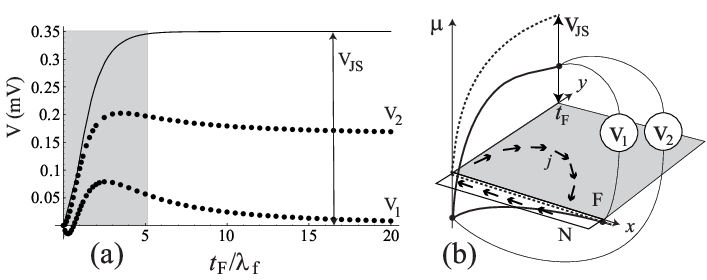
Induced electric current significantly alters the voltage measured in a Johnson-Silsbee experiment and makes it dependent on the position of the voltmeter probe. Let us assume that the F-probe is attached at the top of the F-layer, right above the injection point. For an extended F-electrode, the easiest way to attach an N-probe is at $x_{N}\to\infty$ (Fig. 4, b). Then the measured voltage $V_{1}(t_{F})=\mu(0,t_{F})-\mu(x_{N},0)\to\mu(0,t_{F})$. The plot of $V_{1}(t_{F})$ is given in Fig. 4(a). If the N-probe is attached close to the spin-injection point, the voltage changes to $V_{2}$. Both $V_{1}$ and $V_{2}$ significantly differ from the voltage that would develop in the absence of electric current (solid line in Fig. 4-a). Dependence on the F-electrode thickness is also quite visible even for $t_{F}\gg\lambda_{f}$. The $j=0$ situation emerges either in a narrow F-electrode, or, more generally, in devices where spin is injected uniformly across the F/N interface: According to the Eq. (5), when $\nabla\mu^{s}$ is normal to the boundary, the reason for current generation vanishes together with ${\rm curl}\,{\bf j}$. Uniform spin injection generates voltage that approaches the Johnson and Silsbee result $V_{\rm JS}=(p/2)\mu^{s}_{0}=0.35$ mV for $y\gg\lambda_{f}$.

Spin current tends to decay exponentially with the distance from the injection point. For example, for a non-magnetic top layer, in the present case of $Rt_{N}\gg\lambda_{f}$, we find $a_{k}\approx 1/(f(0)+\lambda_{n}^{2}k^{2})$. Hence, along the interface the spin potential falls off as $\mu^{s}(x,0)\approx\mu^{s}_{0}\exp{(-x/\lambda_{\|})}$. The decay length $\lambda_{\|}=\lambda_{n}/\sqrt{f(0)}$ is bound as per $\lambda_{f}<\lambda_{\|}<\lambda_{n}$. Physically, this means that spins would propagate through a detached normal metal film up to a length of about $\lambda_{n}$, but the spin current leakage into the overlayer shortens their reach.

For a magnetic top layer ($p\neq 0$), a log plot of $\mu^{s}(x,0)$ is shown in Fig. 5: the $\mu^{s}(x,0)$ decays exponentially. However, the decay length crosses over from $\lambda_{\|}$ at $x\ll t_{F}$ to a longer length $\lambda_{c}$ at $x\gg t_{F}$. In the thick-film limit, $Rt_{N}/t_{F}\ll 1$, we find

For the parameters above, this yields $\lambda_{c}\approx 84$ nm against the numerically found $\lambda_{c}\approx 83$ nm.

The $\lambda_{c}$ grows with $t_{F}$ and, at $t_{F}\to\infty$, the $\mu^{s}(x,0)$ decays non-exponentially for $x\gg\lambda_{\|}$. In this limit, $\tanh(t_{F}k)\to{\rm sgn}(k)$ is non-analytic at $k=0$, and the expressions for $F(k)$ and $H(k)$ read

The singularity shows itself as a $|k|^{3}$ term in the expansion of $a_{k}$. Using the stationary phase method, we find an asymptotic expression

with $C=s(p^{2}/(1-p^{2}))(6R^{2}/\pi f^{2}(0))\lambda_{mix}^{2}t_{N}$. Thus, for infinite $t_{F}$, the spin accumulation ultimately decays as a power-law, i.e., very slowly (the blue line in the Fig. 5).

Our findings mean that a ferromagnetic overlayer makes the injected spin current propagate further along the normal film. This conclusion sounds pronouncedly counter-intuitive: After all, ferromagnetic layer is known to be a spin sink, so one would expect that it could only lower the spin propagation length. The seeming paradox is resolved as follows. As we know, the electric current loops cross the F/N boundary. Upon such crossing, a non-equilibrium spin density is inevitably produced [3], so $\mu^{s}$ cannot decay independently of $\bf j$. Ultimately, the conservation of $\bf j$, expressed by the first equation (1), causes a long-range propagation of both charge and spin. The current-assisted propagation of spin also explains the role of the F-layer thickness. The long-range pattern of $\bf j$ is limited by the outer boundaries of the device. Finite $t_{F}$ is equivalent to “covering the fountain by a lid”, deflecting $\bf j$ down to the normal film within a distance of the order of $t_{F}$. Beyond this distance, the power-law decay of spin accumulation reverts to the exponential form.

In conclusion, we have shown that the gradient of spin accumulation along an F/N interface produces closed electric current loops. The first consequence of this is a significant reduction of the Johnson-Silsbee voltage, which means that the interpretation of some non-local resistance experiments with wide F-electrodes may need to be revisited. For example, in the Refs. 15, 16, 17, 18, the current polarization of permalloy was deduced to be $p\lesssim 0.3$, which is significantly smaller than $p\approx 0.7$ inferred from GMR measurements.[19, 20, 21, 8] Such a seeming reduction of $p$ may arise due to loop currents; this can be verified by voltage measurements on a series of devices with varying thickness or width of the F-electrodes.

Alternatively, loop currents will manifest themselves by non-zero voltage drop along the normal film. In the absence of electric current, such a voltage must vanish — but not if ${\bf j}\neq 0$. In particular, if one probe is connected at $x_{N}\to\infty$ and another at $x_{N}=0$, the voltmeter will read off the voltage difference $V_{2}-V_{1}$, shown in Fig. 4.

Another consequence of loop currents is the long-range propagation of spin accumulation along the F/N interface. This effect can be measured by an additional F-electrode positioned downstream of the wide F-electrode. The non-local voltage on the former will reflect the enhanced propagation of spins brought about by the latter. Notice that the signal to be expected in such an experiment is small: As shown in Fig. 5, spin accumulation drops by orders of magnitude before the long-range propagation regime becomes sufficiently pronounced.

More generally, electric current vortices at the interface between two materials shall be expected whenever electric current is coupled to another driven diffusive current by linear relationships with material-dependent Onsager cross-coefficients. For example, coupling with heat flow may induce electric current loops in spin-caloritronic devices with a temperature gradient along the interface between detector ferromagnet and a normal wire.[22, 23, 24]

Ya. B. was supported by the NSF grant DMR-0847159. He is grateful to Laboratoire de Physique Théorique, Toulouse, for the hospitality, and to CNRS for funding the visits.

References

- [1] Spin current, Eds. S. Maekawa, S. O. Valenzuela, E. Saitoh, and T. Kimura, Oxford University Press (2012).
- [2] M. Johnson and R. H. Silsbee, Interfacial charge-spin coupling: Injection and detection of spin magnetization in metals, Phys. Rev. Lett. 55 1790 (1985).
- [3] P. C. van Son, H. van Kempen, and P. Wyder, Boundary resistance of the ferromagnetic-normal metal interface, Phys. Rev. Lett. 58, 2271 (1987).
- [4] T. Valet and A. Fert, Theory of the perpendicular magnetoresistance in magnetic multilayers, Phys. Rev. B 48, 7099 (1993).
- [5] S. Takahashi and S. Maekawa, Spin injection and detection in magnetic nanostructures, Phys. Rev. B 67, 052409 (2003).
- [6] E. I. Rashba, Theory of electrical spin injection: Tunnel contacts as a solution of the conductivity mismatch problem, Phys. Rev. B 62, R16267 (2000).
- [7] E. I. Rashba, Diffusion theory of spin injection through resistive contacts, Eur. Phys. J. B 29 513 (2002).
- [8] J. Hamrle, T. Kimura, Y. Otani, K. Tsukagoshi, and Y. Aoyagi, Current distribution inside Py/Cu lateral spin-valve devices, Phys. Rev. B 71, 094402 (2005).
- [9] In the Refs. 8, 10, 11, they do.
- [10] M. Johnson and R. H. Silsbee, Calculation of nonlocal baseline resistance in a quasi-one-dimensional wire, Phys. Rev. B 76, 153107 (2007).
- [11] R. Nakane, S. Sato, S. Kokutani, and M. Tanaka, Appearance of Anisotropic Magnetoresistance and Electric Potential Distribution in Si-Based Multiterminal Devices With Fe Electrodes, IEEE Magn. Lett. 3, 3000404 (2012).
- [12] Currents are defined here as particle number currents. Electric currents are obtained by multiplying by electron charge.
- [13] T. Kimura, Y. Otani, and J. Hamrle, Switching magnetization of nanoscale ferromagnetic particle using nonlocal spin injection, Phys. Rev. Lett. 96, 037201 (2006).
- [14] T. Kimura, Y. Otani, Large spin accumulation in permalloy-silver lateral spin valve, Phys. Rev. Lett. 99, 196604 (2007).
- [15] F. J. Jedema, A. T. Filip, and B. J. van Wees, Electrical spin injection and accumulation at room temperature in an all-metal mesoscopic spin valve Nature 410, 345 (2001).
- [16] F. J. Jedema, M. S. Nijboer, A. T. Filip, and B. J. van Wees, Spin injection and spin accumulation in all-metal mesoscopic spin valves Phys. Rev. B 67, 085319 (2003).
- [17] T. Kimura and Y. Otani, Spin transport in lateral ferromagnetic/nonmagnetic hybrid structures, J. Phys.: Condens. Matter 19, 165216 (2007).
- [18] M. Erekhinsky, A. Sharoni, F. Casanova, and I. K. Schuller, Surface enhanced spin-flip scattering in lateral spin valves, Appl. Phys. Lett. 96, 022513 (2010).
- [19] S. D. Steenwyk, S. Y. Hsu, R. Loloee, J. Bass, and W. P. Pratt, Jr. Perpendicular-current exchange-biased spin-valve evidence for a short spin-diffusion length in permalloy, J. Magn. Magn. Mater. 170, L1 (1997).
- [20] P. Holody, W. C. Chiang, R. Loloee, J. Bass, W. P. Pratt, Jr., and P. A. Schroeder, Giant magnetoresistance of copper/permalloy multilayers, Phys. Rev. B 58, 12230 (1998).
- [21] S. Dubois, L. Piraux, J. M. George, K. Ounadjela, J. L. Duvail, and A. Fert, Evidence for a short spin diffusion length in permalloy from the giant magnetoresistance of multilayered nanowires, Phys. Rev. B 60 477 (1999).
- [22] F. L. Bakker, A. Slachter, J.-P. Adam, and B. J. van Wees, Interplay of Peltier and Seebeck Effects in Nanoscale Nonlocal Spin Valves, Phys. Rev. Lett. 105, 136601 (2010).
- [23] A. Slachter, F. L. Bakker, J-P. Adam, and B. J. vanWees, Thermally driven spin injection from a ferromagnet into a non-magnetic metal, Nat. Phys. 6, 879 (2010).
- [24] M. Erekhinsky, F. Casanova, I. K. Schuller, and A. Sharoni Spin-dependent Seebeck effect in non-local spin valve devices, Appl. Phys. Lett. 100, 212401 (2012).