Asymptotic analysis of solutions to transmission problems in solids with many inclusions

Uniform asymptotic approximations for solutions to boundary value problems involving large clusters of small defects have been constructed in the articles [20, 24, 26, 27] and the monograph [25]. The approximations have been developed for different operators of mathematical physics and for a range of different boundary conditions imposed on the surfaces of the small defects. The approach employed in achieving these approximations does not utilise any strong assumptions on the arrangements of inclusions within the cluster, such as periodically distributed defects or arrangements which are statistically determined, where alternative conventional techniques such homogenisation are applicable [2, 15].

Here we address the approximation of the solution to a transmission problem for a solid containing a dense non-periodic arrangement of small inclusions. In particular, such an approximation is capable of tracing the interaction of defects within a cluster, which is a serious challenge, especially in regions where fields are likely to rapidly oscillate.

Several important approximations for solids containing dilute arrangements of defects, amongst much else, have appeared in [30, 31]. There, the method of compound asymptotic expansions is systematically presented for various elliptic boundary value problems of mathematical physics in singularly perturbed domains. For domains with small defects, the method relies on model problems posed in domains without any holes, and problems in the exterior of individual small defects. The approach has also led to approximations for energy characteristics associated with these singularly perturbed problems in perforated domains such as eigenvalues, stress-intensity factors and capacities.

The method of compound asymptotic expansions has recently played a major role in uniform asymptotic approximations for Green’s kernels in domains with several defects for both scalar [16, 17, 18, 19] and vector problems [21, 22]. In particular, a uniform approximations to singular fields for transmission problems in planar bodies containing several small inclusions has appeared in [23]. Approximations of this type have been shown to provide results that give excellent comparison with those based on benchmark finite element schemes [21, 23]. Uniform asymptotic approximations for Green’s functions have also been used to model the flow of obstacles in Hele-Shaw flow [32, 34].

The approximations mentioned above for dilute composites serve the case when the number of small defects are finite and are situated far apart from each other. However, in the situation when the number of defects becomes large and can be close to each other, one needs an alternative tool to model this scenario.

If the small defects are arranged periodically in some region, then one can employ powerful homogenisation based techniques to model an effective medium [15]. The technique can also reveal additional contributions to the physics of such problems when the number of small particles within the region increase, while the overall volume occupied within a region remains constant [8, 15]. Periodic composite materials for both electromagnetism and elasticity have been modelled using the homogenisation approach in [36] and has been extended to treat problems where different boundary conditions are supplied on neighboring defects in [10]. This averaging procedure has led to the effective properties of cubically arranged homogeneous spherical inclusions in an ambient matrix in [11] and for homogenisation to periodic elastic media with jumps in the transmission conditions on interfaces of small inclusions, see [33].

Other approaches used to establish effective behaviour of composites include a potential approach used in [12] to determine the effective conductivity for dense arrays of perfectly conducting spheres or perfectly and non-perfectly conducting cylinders. In addition, a functional equation approach has been used to study the effective conductivity of doubly periodic systems of inclusions distributed within a matrix having non-ideal contact conditions in two dimensions [5].

In addition, the homogenisation technique can treat composites where defect positions do not exhibit periodicity, but may be specified by some statistical law. For example, see [3] for a problem of this type that considers the potential for medium containing randomly distributed circular inclusions under ideal contact conditions. In [13, 14, 35], homogenisation based approximations have been used to obtain estimates of effective moduli characterising the composites for both elastic and hyperelastic materials containing randonly distributed fibres or defects. For the case of a Neo-Hookean material containing periodically placed fibers that is subjected to different loading conditions, see [4].

Naturally, one can find many examples of densely perforated materials for which the position of the perforations are not governed by periodicity or a statistical law. Hence a homogenisation approach is not applicable when modelling these materials.. The method of meso-scale asymptotic approximations was developed in [20] to approximate potentials for a bodies containing large non-periodic clusters of small defects, with rigid boundaries. Meso-scale approximations for solids containing a cluster of voids has appeared in [24]. More recently, the meso-scale approach has been used to approximate solutions for problems of the Lamé system for three-dimensional solids with clouds of defects with rigid boundaries in [26] and when the traction-free conditions are supplied on small voids [27].

Low-frequency vibration problems for solids with arrays of small inclusions have also been addressed using a modification of the methods of compound and meso-scale asymptotic approximations. Asymptotics of the first eigenvalue and corresponding eigenfunction for domains with a cloud of rigid inclusions have appeared in [28]. Applications of the method of meso-scale approximations have also appeared in [6, 7], where the scattering problems for many small obstacles in the infinite space were considered.

Here we adapt the approaches of [25] and [30, 31] to develop the approximation of the solution to a transmission problem inside a body with many small arbitrary inclusions. Before stating the main result of this article, we supply the details of the problem we intend to tackle. Here, $\Omega$ will denote a bounded subset of $\mathbb{R}^{3}$, which we assume contains a material with shear modulus $\mu_{O}$ and has smooth boundary $\partial\Omega$. Let $\omega$ be a region of $\Omega$, with diameter $1$. Contained in $\omega$ will be many small inclusions $\omega_{\varepsilon}^{(k)}$, $1\leq k\leq N$. The $k^{th}$ inclusion has centre ${\bf O}^{(k)}$, a smooth interface $\partial\omega_{\varepsilon}^{(k)}$, a normalized diameter which is characterized by the small dimensionless parameter $\varepsilon$, and is also occupied by a material with shear modulus $\mu_{I_{k}}$, $1\leq k\leq N$. Another small non-dimensional parameter $d$, defined by

is used to illustrate the “closeness” of one inclusion to the other within the cloud $\omega$. Additional geometric constraints on $\omega$ are then given by

The parameters $N$ and $d$ satisfy the inequality

Our main objective is to derive the asymptotic approximation to the displacement function $u_{N}$ satisfying the transmission problem

where $\partial\omega_{\varepsilon}^{(j)+}$ ($\partial\omega_{\varepsilon}^{(j)-}$) represents the boundary $\partial\omega^{(j)}_{\varepsilon}$ approached from the exterior (interior). The function $f$,describing the body force in $\Omega_{N}$, belongs to the space $L_{2}(\Omega)$, and has a support satisfying $\omega\cap\text{supp }f=\varnothing$ and $\text{dist}(\omega,\text{supp }f)=O(1)$. In the displacement condition on $\partial\Omega$ we have $\phi\in L^{1/2,2}(\partial\Omega)$.

The construction of the asymptotics of $u_{N}$ relies on the methods of compound and meso-scale asymptotic expansions, which in turn makes use of model fields defined in the unperturbed set (without small inclusions) $\Omega$ and in the infinite space containing a single small inclusion $\omega_{\varepsilon}^{(k)}$, $k=1,\dots,N$. Such model fields involve:

1. 1.

   the solution $w_{f}$ of the Dirichlet problem of Poisson’s equation in $\Omega$;

2. 2.

   the vector functions ${\mbox{\boldmath${\cal D}$}}^{(k)}_{\varepsilon}$, whose components are the dipole fields for the inclusion $\omega_{\varepsilon}^{(k)}$. These fields allow one to construct boundary layers outside small holes in the asymptotic algorithm;

3. 3.

   the regular part $H$ of Green’s function $G$ in $\Omega$.

It will also be shown that coefficients near boundary layers in the approximation of $u_{N}$ form solutions to a certain algebraic system. This system involves derivatives of $w_{f}$ and integral characteristics pertaining to the small voids such as the polarization matrix ${\mbox{\boldmath${\cal P}$}}^{(k)}_{\varepsilon}$, (see [29]) which is a $3\times 3$ matrix for the small inclusions $\omega_{\varepsilon}^{(k)}$, $1\leq k\leq N$. As is discussed in more detail later, this matrix can be positive or negative definite. In addition, if ${\mbox{\boldmath${\cal P}$}}^{(k)}_{\varepsilon}$ is negative (positive) definite, we assume that the maximum and minimum eigenvalues $\lambda^{(j)}_{\text{max}}$ and $\lambda^{(j)}_{\text{min}}$, respectively, of $-{\mbox{\boldmath${\cal P}$}}^{(j)}_{\varepsilon}$ (${\mbox{\boldmath${\cal P}$}}^{(j)}_{\varepsilon})$ satisfy

where $C_{1}$ and $C_{2}$ are constants independent of $\varepsilon$.

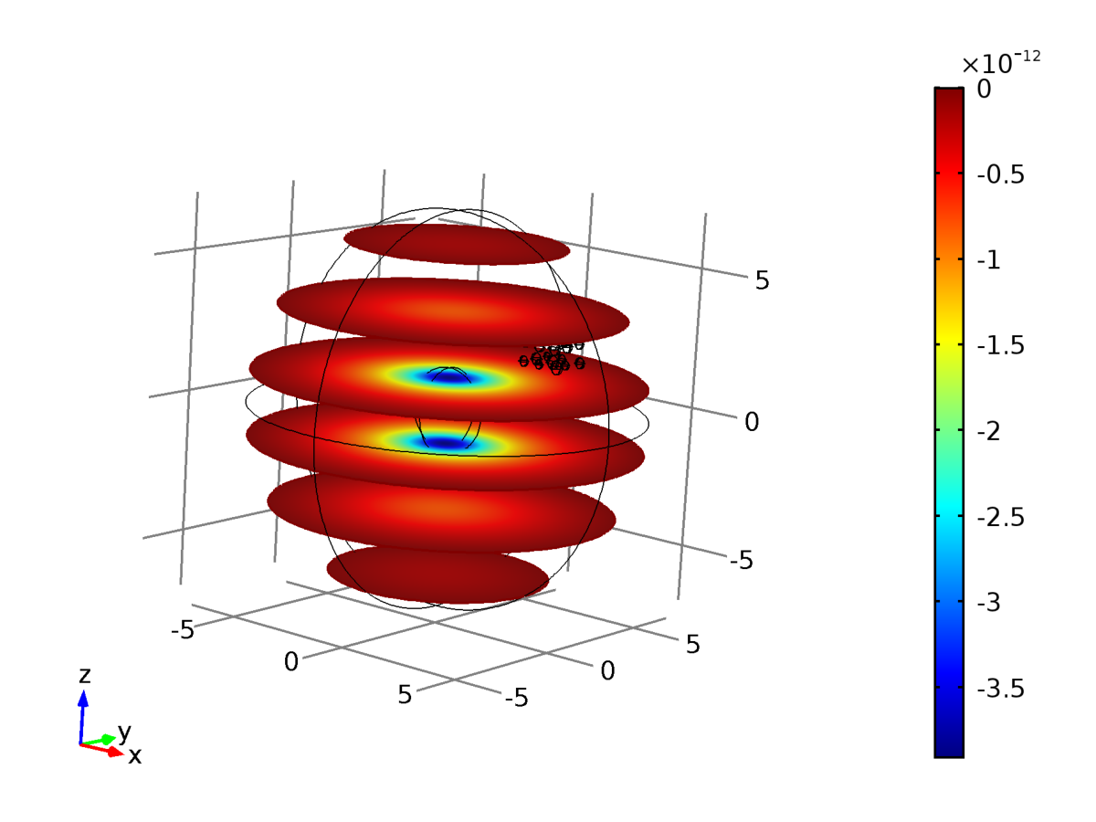
As an example, we consider a large cluster of inclusions ($N=64$) arranged in cube, as according to Figure 1, which is embedded in sphere of radius 7. Here $f({\bf x})$ in (1.1) is a radially symmetric function having support inside the ball of radius 1.5 (further details of the numerical set up can be found in section 8). The cluster is composed of both voids and inclusions which are occupied by either Cast Iron, Steel AISI 4340, Aluminum, Copper or Iron. The ambient matrix has the material properties of Structural Steel. For such a problem, the task of using the method of finite elements, with the package COMSOL, to obtain the solution $u_{N}$ can be computationally intensive. In fact, COMSOL could not compute the solution to this problem in this case. However, the asymptotic formulae (1.4) remains efficient and we present computations for $|\nabla u_{N}|$, based on the derivatives of the leading order approximation to $u_{N}$ in (1.4), along cut-planes which intersect the cloud.

The structure of the article is as follows. In section 2 we introduce model problems which allow one to construct the formal approximation to $u_{N}$, and this formal asymptotic procedure is provided in section 3. There, the algebraic system, concerning coefficients involved in the asymptotic approximation to $u_{N}$, is determined and the solvability of this system is discussed in section 4. The proof of the energy estimate (1.6) for the remainder term involved in the approximation is provided in section 5, where the completion of the proof of Theorem 1 is also presented. In section 6, we extend the results of Theorem 1 to the case of the transmission problem for an infinite medium containing a non-periodic cluster of small inclusions. Following this, in section 7, we further investigate the algebraic system (1.5) for a large periodic cluster situated inside a body and from this we derive an auxiliary homogenised problem concerning the effective inclusion $\omega$ situated inside the domain $\Omega$. Numerical illustrations are then given in section 8 that show the efficiency of the asymptotic approach, in particular, when compared with computations based on finite element algorithms. In section 9, we give some conclusions and discussion. Finally, in the Appendix, we present the proofs of auxiliary results needed to prove the solvability of the algebriac system discussed in section 4.

We now introduce model problems posed in either the unperturbed domain $\Omega$ or the infinite space with the small inclusion at the origin, which we use in the formal asymptotic procedure given in the following section.

1. $1.$

   The solution $w_{f}$ of the Dirichlet problem for Poisson’s equation. Let $w_{f}$ satisfy the problem

   $$\mu_{O}\Delta w_{f}({\bf x})=f({\bf x})\;,\quad{\bf x}\in\Omega\;,$$

   (2.1)

   $$w_{f}({\bf x})=\phi({\bf x})\;,\quad{\bf x}\in\partial\Omega\;,$$

   where as before $f\in L_{2}(\Omega)$, $\text{supp }f\cap\omega=\varnothing$, $\text{dist}(\omega,\text{supp }f)=O(1)$ and $\phi\in L^{1/2,2}(\partial\Omega)$. Later, we assume that $f$ is extended by zero inside the inclusions $\omega^{(k)}_{\varepsilon}$, $1\leq k\leq N$.

2. $2.$

   The regular part $H$ in $\Omega$. Let $H$ be the regular part of Green’s function $G$ in $\Omega$, which satisfies

   $$\mu_{O}\Delta_{\bf x}H({\bf x},{\bf y})=0\;,\quad{\bf x},{\bf y}\in\Omega\;,$$

   $$H({\bf x},{\bf y})=(4\pi\mu_{O}|{\bf x}-{\bf y}|)^{-1}\;,\quad{\bf x}\in\partial\Omega\;,{\bf y}\in\Omega\;,$$

   (2.2)

   and $G$ is related to $H$ via

   $$H({\bf x},{\bf y})=\frac{1}{4\pi\mu_{O}|{\bf x}-{\bf y}|}-G({\bf x},{\bf y})\;.$$

   (2.3)

3. $3.$

   The dipole fields for the small inclusion $\omega_{\varepsilon}^{(j)}$, $j=1,\dots,N$. The dipole fields $\mathcal{D}^{(k)}_{j}$, $j=1,2,3$, for the scaled inclusion $\omega^{(k)}=\{\mbox{\boldmath${\xi}$}:\varepsilon\mbox{\boldmath${\xi}$}+{\bf O}^{(j)}\in\omega_{\varepsilon}^{(k)}\}$, are now introduced as components of the vector function ${\mbox{\boldmath${\cal D}$}}^{(k)}=(\mathcal{D}^{(k)}_{1},\mathcal{D}^{(k)}_{2},\mathcal{D}^{(k)}_{3})^{T}$, $k=1,\dots,N$, which solves the transmission problem

   $$\left.\begin{array}[]{c}\mu_{O}\displaystyle{\Delta{\mbox{\boldmath${\cal D}$}}^{(k)}(\mbox{\boldmath${\xi}$})={\bf O}\;,\quad\mbox{\boldmath${\xi}$}\in\mathbb{R}^{3}\backslash\overline{\omega^{(k)}}\;,}\\ \\ \mu_{I_{k}}\displaystyle{\Delta{\mbox{\boldmath${\cal D}$}}^{(k)}(\mbox{\boldmath${\xi}$})={\bf O}\;,\quad\mbox{\boldmath${\xi}$}\in\omega^{(k)}\;,}\\ \\ \displaystyle{{\mbox{\boldmath${\cal D}$}}^{(k)}(\mbox{\boldmath${\xi}$})\Big|_{\partial\omega^{(k)+}}={\mbox{\boldmath${\cal D}$}}^{(k)}(\mbox{\boldmath${\xi}$})\Big|_{\partial\omega^{(k)-}}\;,}\\ \\ \displaystyle{\mu_{O}\frac{\partial{\mbox{\boldmath${\cal D}$}}^{(k)}}{\partial n}(\mbox{\boldmath${\xi}$})\Big|_{\partial\omega^{(k)+}}-\mu_{I_{k}}\frac{\partial{\mbox{\boldmath${\cal D}$}}^{(k)}}{\partial n}(\mbox{\boldmath${\xi}$})\Big|_{\partial\omega^{(k)-}}=(\mu_{O}-\mu_{I_{k}})\boldsymbol{n}^{(k)}\;,}\end{array}\right\}$$

   (2.4)

   where $\boldsymbol{n}^{(k)}$ is the unit outward normal to $\omega^{(k)}$. The leading order behaviour of ${\mbox{\boldmath${\cal D}$}}^{(k)}$, described in (2.4), can be written explicitly using the $3\times 3$ symmetric polarization matrix ${\mbox{\boldmath${\cal P}$}}^{(k)}=\{{\cal P}_{ij}^{(k)}\}_{i,j=1}^{3}$ for the small inclusion. We have

   Lemma 1

   $($see [29]$)$ Let $|\mbox{\boldmath${\xi}$}|>2$, then the vector function ${\mbox{\boldmath${\cal D}$}}^{(k)}$ admits the asymptotic representation

   $${\mbox{\boldmath${\cal D}$}}^{(k)}(\mbox{\boldmath${\xi}$})=-{\mbox{\boldmath${\cal P}$}}^{(k)}\nabla((4\pi\mu_{O}|\mbox{\boldmath${\xi}$}|)^{-1})+O(|\mbox{\boldmath${\xi}$}|^{-3})\;,$$

   (2.5)

   where the entries of ${\mbox{\boldmath${\cal P}$}}^{(k)}=[{\cal P}^{(k)}_{ij}]_{i,j=1}^{3}$ are given by

   	$\displaystyle{\cal P}^{(k)}_{ij}$	$\displaystyle=$	$\displaystyle(\mu_{I_{k}}-\mu_{O})\text{{\rm meas\rm}}(\omega^{(k)})\delta_{ij}-\mu_{O}\int_{\mathbb{R}^{3}\backslash\overline{\omega^{(k)}}}\nabla\mathcal{D}^{(k)}(\mbox{\boldmath${\xi}$})\cdot\nabla\mathcal{D}^{(j)}(\mbox{\boldmath${\xi}$})d\mbox{\boldmath${\xi}$}$		(2.6)
   			$\displaystyle-\mu_{I_{k}}\int_{\omega^{(k)}}\nabla\mathcal{D}^{(k)}(\mbox{\boldmath${\xi}$})\cdot\nabla\mathcal{D}^{(j)}(\mbox{\boldmath${\xi}$})d\mbox{\boldmath${\xi}$}\;,$

   for $1\leq i,j\leq 3$.

Here, the expression (2.6) shows that the polarization matrix ${\mbox{\boldmath${\cal P}$}}^{(k)}$ is symmetric. Further, after integration by parts and using the definition (2.4) of the components of the vector function ${\cal D}$ one can show that

where further integration by parts in $\omega^{(k)}$ in the term on the right gives

As a result the integral term in (2.7) defines a Gram matrix. Here (2.7) shows that for voids ($\mu_{I_{k}}=0$) the dipole matrix is negative definite, whereas if $\mu_{I_{k}}>\mu_{O}$ ($\mu_{I_{k}}<\mu_{O}$), this polarization tensor is positive (negative) definite.

By then rescaling, we create the vector functions ${\mbox{\boldmath${\cal D}$}}^{(j)}_{\varepsilon}({\bf x})=\varepsilon{\mbox{\boldmath${\cal D}$}}(\varepsilon^{-1}({\bf x}-{\bf O}^{(j)}))$ and matrices ${\mbox{\boldmath${\cal P}$}}^{(j)}_{\varepsilon}=\varepsilon^{3}{\mbox{\boldmath${\cal P}$}}^{(j)}$, $1\leq j\leq N$, which are to be used throughout the asymptotic algorithm. Here, the components of ${\mbox{\boldmath${\cal D}$}}^{(j)}_{\varepsilon}$ are then the dipole fields for the inclusion $\omega^{(k)}_{\varepsilon}$, $1\leq k\leq N$.

We now formally construct an asymptotic approximation to the solution $u_{N}$ of the transmission problem (1.1). We prove the following Lemma.

Proof. We first attempt to satisfy the governing equations in $\bigcup_{j=1}^{N}\omega_{\varepsilon}^{(j)}\cup\Omega_{N}$ and the exterior boundary condition appearing in (1.1). Therefore, we approximate $u_{N}$ by the field $w_{f}$ defined in $\Omega$, i.e.

Considering the boundary value problem for $W_{N}$, we have

Since $w_{f}$ is defined everywhere in $\Omega$, $W_{N}$ is continuous across the frontier $\partial\omega_{\varepsilon}^{(j)}$, $j=1,\dots,N$. However, the jump in the traction condition across $\partial\omega_{\varepsilon}^{(j)}$, $j=1,\dots,N$, is

Since the inclusion $\omega_{\varepsilon}^{(j)}$, $j=1,\dots,N$, is small, we can use Taylor’s expansion of the derivatives of $w_{f}$ about $\mathbf{O}^{(j)}$ in the preceding condition, to obtain

We now use the notion of the dipole fields for the inclusions (see Problem 3, Section 2) to compensate for the error in the above right-hand side and construct $W_{N}$ with the representaion

where in subsequent steps we will identify the algebraic system satidfied by ${\bf C}^{(k)}=(C_{1}^{(k)},C_{2}^{(k)},C_{3}^{(k)})^{T}$, $k=1,\dots,N$.

Then, the field $R_{N}$ is harmonic inside $\Omega_{N}$ and $\omega_{\varepsilon}^{(j)}$, $j=1,\dots,N$. The asymptotics of ${\mbox{\boldmath${\cal D}$}}^{(k)}_{\varepsilon}$, (see Lemma 1), and the boundary condition (2.2) for $H$, allow one to assert that

On the other hand, the same far-field representation for ${\mbox{\boldmath${\cal D}$}}_{\varepsilon}^{(k)}$, $k\neq j$, in (3.2) provides the displacement condition

and the traction condition (see (3.2))

Next, we expand the second order derivatives of $G$ about ${\bf x}={\bf O}^{(j)}$, to give

Inspecting the last condition then suggests that ${\bf C}^{(k)}$, $1\leq j\leq N$ should satisfy

to allow for the removal of the leading order discrepancy in the preceding traction condition. Finally, combining (3.1) and (3.3)–(3.6) completes the proof of Lemma 2. $\Box$

Here we prove a result concerning the solvability of the algebraic system (3.6).

We postpone the proof of this Lemma, in order to rewrite the algebraic system in a way which will simplify its representation, and we give some auxiliary results.

Here, in several steps, we prove the next lemma.

References

- [2] N. S. Bakhvalov and G. Panasenko (1989), Homogenization: Averaging Processes in Periodic Media, Springer, Berlin.
- [3] L. Berlyand, V. Mityushev, (2001): Generalized Clausius–Mossotti Formula for Random Composite with Circular Fibers, Journal of Statistical Physics 102, no. 1, 115–145.
- [4] M. Brun, O. Lopez-Pamies, P. Ponte Castañeda (2007): Homgenization estimates for fiber-reinforced elastomers with periodic microstructures, Internation Journal of Solids and Structures 44, 5953–5979.
- [5] L.P. Castro, E. Pesetskaya and S.V. Rogosin (2009): Effective Conductivity of a Composite Material with Non-ideal Contact Conditions, Complex Variables and Elliptic equations 54, no. 12, 1085–1100.
- [6] D.P. Challa and M. Sini: On the justification of the Foldy-Lax approximation for the acoustic scattering by small rigid bodies of arbitrary shapes. Multiscale Model. Simul. 12, no. 1 55-108, (2014).
- [7] D.P. Challa and M. Sini.: Multiscale analysis of the acoustic scattering by many scatterers of impedance type. Z. Angew. Math. Phys. 67:58, (2016).
- [8] D. Cioranescu and F. Murat: A strange term brought from somewhere else, Nonlinear Partial Differential Equations and their Applications, Colleg̀e de France Seminar, III, Research Notes in Mathematics Vol. 70 (A K Peters, Natick, MA, 1982), pp. 154–178.
- [9] D. Gilbarg, N.S. Trudinger (2001): Elliptic Partial Differential Equations of Second Order, Springer.
- [10] W. Jäger, O.A.Oleinik, T.A. Shaposhnikova: On homogenization of solutions of the poisson equation in a perforated domain with different types of boundary conditions on different cavities, Applicable Analysis: An international journal 65, no. 3–4, 205–223.
- [11] G. Kristensson (2003), Homogenization of spherical inclusions, Progress in Electromagnetics Research 42, 1–25.
- [12] J.B. Keller, (1963): Conductivity of a medium containing a dense array of perfectly conducting spheres or cylinders or nonconducting cylinders, Journal of Applied Physics 34, no. 4, (1).
- [13] O. Lopez-Pamies, P. Ponte Castañeda (2006): On the overall behavior, microstructure evolution, and macroscopic stability in reinforced rubbers at large deformations: I–Theory, Journal of the Mechanics and Physics of Solids 54, 807–830.
- [14] O. Lopez-Pamies, P. Ponte Castañeda (2006): On the overall behavior, microstructure evolution, and macroscopic stability in reinforced rubbers at large deformations: II–Application to cylindrical fibers, Journal of the Mechanics and Physics of Solids 54, 831–863.
- [15] V. A. Marchenko and E. Y. Khruslov (2006), Homogenization of Partial Differential Equations, Birkhäuser, Basel.
- [16] V. Maz’ya and A. Movchan (2006), Uniform asymptotic formula for regularly and singularly perturbed domains, C. R. Math. Acad. Sci. Paris 343, No. 3, 185–190.
- [17] V. Maz’ya and A. Movchan (2007), Uniform asymptotic formulae for Green’s functions in singularly perturbed domains, J. Comput. Appl. Math. 208, No. 1, 194–206.
- [18] V. Maz’ya and A. Movchan (2008), Uniform asymptotic approximations of Green’s function in a long rod, Math. Methods Appl. Sci. 31, No. 17, 2055–2068.
- [19] V. Maz’ya and A. Movchan (2009), Uniform asymptotics of Green’s kernels for mixed and Neumann problems in domains with small holes and inclusions. Sobolev spaces in mathematics. III, pp. 277-213, In: Sobolev Spaces in Mathematics. III. Applications in Mathematical Physics, Springer and Tamara Rozhkvoskaya Publisher, New York.
- [20] V. Maz’ya and A. Movchan (2010), Asymptotic treatment of perforated domains without homogenization, Math. Nachr. 283, No. 1, 104–125.
- [21] V. Maz’ya, A. Movchan, and M. Nieves, Uniform asymptotic formulae for Green’s tensors in elastic singularly perturbed domains with multiple inclusions, Rend. Accad. Naz. Sci. XL Mem. Mat. Appl. 5, No. 30, 103–157 (2006).
- [22] V. G. Maz’ya, A. B. Movchan, and M. J. Nieves, Uniform asymptotic formulae for Green’s tensors in elastic singularly perturbed domains, Asymptot. Anal. 52, No. 3-4, 173–206, (2007).
- [23] V. Maz’ya, A. Movchan, and M. Nieves, Green’s kernels for transmission problems in bodies with small inclusions, In: Operator Theory and Its Applications, pp. 127–160, Am. Math. Soc., Providence, Ri (2010).
- [24] V. Maz’ya, A. Movchan, and M. Nieves (2011): Mesoscale asymptotic approximations to solutions of mixed boundary values problems in perforated domains, Multiscale Model. Simul. 9, No. 1, 424–448.
- [25] V. Maz’ya, A. Movchan and M. Nieves, (2013): Green’s Kernels and Meso-Scale Approximations in Perforated Domains, Lecture Notes in Mathematics 2077, Springer.
- [26] V. Maz’ya, A. Movchan, and M. Nieves (2014), “Mesoscale approximations for solutions of the Dirichlet problem in a perforated elastic body,” Journal of Mathematical Sciences 202, no.2, 215–254.
- [27] V. Maz’ya, A. Movchan, and M. Nieves (2016), Meso-scale models and approximate solutions for solids containing clouds of voids, SIAM: Multiscale Modelling and Simulation, 14, no. 1, 138–172.
- [28] V. Maz’ya, A. Movchan, and M. Nieves (2016), Eigenvalue problem in a solid with many inclusions: asymptotic analysis, ArXiv preprint, arXiv:1606.03084
- [29] A. B. Movchan, N. V. Movchan, C. G. Poulton, Asymptotic Models of Fields in Dilute and Densely Packed Composites, Imperial College Press, (2002).
- [30] V. Maz’ya, S. Nazarov, and B. Plamenevskij (2000), Asymptotic Theory of Elliptic Boundary Value Problems in Singularly Perturbed Domains. I, Birkhäuser, Basel.
- [31] V. Maz’ya, S. Nazarov, and B. Plamenevskij (2000), Asymptotic Theory of Elliptic Boundary Value Problems in Singularly Perturbed Domains. II, Birkhäuser, Basel.
- [32] G. Mishuris, S. Rogosin and M. Wrobel (2015): Moving stone in the Hele-Shaw flow. Mathematika 61, no. 2, 457–474.
- [33] J. Orlik (2012): Two-scale homogenization in transmission problems of elasticity with interface jumps, Applicable Analysis 91, no. 7, 1299–1319.
- [34] D. Peck, S.V. Rogosin, M. Wrobel, G. Mishuris (2016): Simulating the Hele-Shaw flow in the presence of various obstacles and moving particles. Meccanica 51, 1041–1055.
- [35] P. Ponte Castañeda, J. R. Willis (1995): The effect of spatial distribution on the effective behaviour of composite materials and cracked media. Journal of the Mechanics and Physics of Solids 43, no. 12, 1919-1951.
- [36] E. Sánchez-Palencia (1980), Non-Homogeneous Media and Vibration Theory, Lecture Notes in Physics 127, Springer.