Dappled tilingThanks: The first author was partially supported by KAKENHI, Grant-in-Aid for Young Scientists (B) 26800043.Thanks: The third author was partially supported by KAKENHI Grant Number 15H03613.
Abstract.
We consider a certain tiling problem of a planar region in which there are no long horizontal or vertical strips consisting of copies of the same tile. Intuitively speaking, we would like to create a dappled pattern with two or more kinds of tiles. We give an efficient algorithm to turn any tiling into one satisfying the condition, and discuss its applications in texturing.
Key words and phrases:
tiling algorithm, texture generation, Brick Wang tiles2010 Mathematics Subject Classification
52C20, 68U051. Introduction
In texturing, we often encounter the following problem: fill a region with a given collection of small square patches in such a way that patches of a same kind do not appear in a row. We make this problem more precise.
Definition 1.1.
For natural numbers and , let be a rectangular grid
We call its elements cells. Our convention is that is the cell at the top-left corner and is at the top-right corner. For a finite set of tiles with , we call a function a tiling of with . For a natural number and , we say satisfies the condition if there is no horizontal strip with more than consecutive ’s, that is, there is no such that . Similarly, we say satisfies the condition for a natural number , if there is no vertical strip with more than consecutive ’s.
Consider a set consisting of conditions of the form and with varying and . Alternatively, we can think of as functions so that . For notational convenience, we allow , which is always satisfied. We will use both notations interchangeably. We say a tiling is -dappled if satisfies all the conditions in . The problem we are concerned is:
Problem 1.2.
Give an efficient algorithm to produce -dappled tilings, which posses some controllability by the user.
In this paper, we introduce an algorithm to produce an -dappled tiling by modifying a given initial tiling which need not be -dappled. Note that enumerating all the -dappled tilings is fairly straightforward; we can fill cells sequentially from the top-left corner. However, this is not practical since there are exponentially many -dappled tilings with respect to the number of cells, and many of them are not suitable for applications as we see below.
Proposition 1.3.
Let . There exist at least tilings which are -dappled.
Proof.
We will create draughtboard tilings. For each cell , choose any tile and put the same tile at (if it exists). Pick any and put them at and (if they exist). One can see that for any the tile at or is different from the one at . Similarly, the tile of or is different from the one at , and hence, the tiling thus obtained is -dappled with any . There are cells of the form , and hence, there are at least draughtboard tilings. ∎
It is easy to see that the above argument actually shows that there are at least draughtboard (and hence, -dappled) tilings with .
Example 1.4.
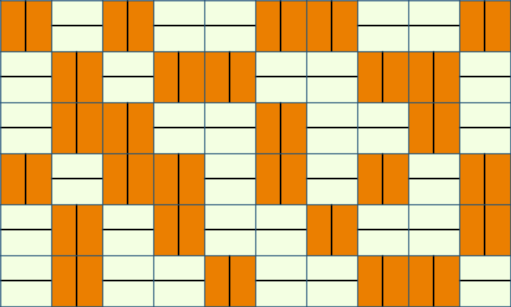
We show an example of a draughtboard tiling with (Fig. 1). For any set of conditions , it is an -dappled tiling.


Draughtboard patters look very artificial and are not suitable for texturing. We would like to have something more natural. Therefore, we consider an algorithm to produce an -dappled tiling which takes a user specified (not necessarily -dappled) tiling as input so that the user has some control over the output. We also discuss a concrete applications with the Brick Wang tiles ([1, 2, 3]) in §4, and with flow generation in §5.
Remark 1.5.
For the special case of and , the numbers of -dappled tilings for several small and are listed at [4]. No formula for general and nor a generating function is known as far as the authors are aware.
2. The algorithm
Fix a set of conditions . We just say dappled for -dappled from now on. Given any tiling , we give an algorithm to convert it into a dappled one. We can start with a random tiling or a user specified one. First, note that the problem becomes trivial when since we can choose a tile for at step (I) below which is different from and . So, we assume consists of two elements .
The idea is to perform “local surgery” on . We say violates the condition (resp. ) at when (resp. ). For a cell we define its weight . Let be a cell with the minimum weight such that violates any of the conditions or . We modify values of around to rectify the violation in the following manner.
- (I).
Set if it does not violate any condition at in .
- (II).
Otherwise, set , and .
Let us take a close look at step (II). Assume that violated at . This means . Note also that since otherwise we could set at step (I). When , we can set without introducing a new violation at . When , we can set and without introducing a new violation at either of or . A similar argument also holds when is violated at .
After the above procedure, the violation at is resolved without introducing a new violation at cells with weight . (We successfully “pushed” the violation forward.) Notice that each time either the minimal weight of violating cells increases or the number of violating cells with the minimal weight decreases. Therefore, by repeating this procedure a finite number of times, we are guaranteed to obtain a dappled tiling transformed from the initially given tiling.
The algorithm works in whatever order the cells of a same weight are visited, but our convention in this paper is in increasing order of . All the examples are produced using this ordering.
Proposition 2.1.
The sub-routine returns true if violates any of horizontal or vertical conditions at the given cell. In practice, the check can be efficiently performed by book-keeping the numbers of consecutive tiles of smaller weight in the horizontal and the vertical directions. See the python implementation [5] for details.
Example 2.2.


Remark 2.3.
Algorithm 1 does not always work when or for some . For example, when it cannot rectify the following tiling of :
3. Extension
We give two extensions of the main algorithm discussed in the previous section.
3.1. Non-uniform condition
It is easy to see that our algorithm works when the conditions and vary over cells. That is, and can be functions of as well as so that . This allows the user more control over the output. For example, the user can put non-uniform constraints, or even dynamically assign constraints computed from the initial tiling.
Example 3.1.
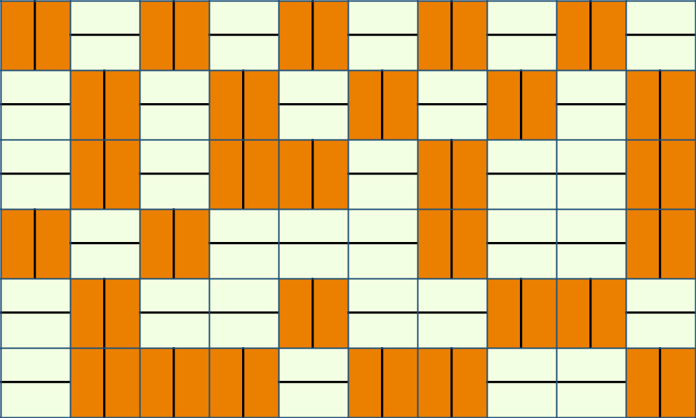
Let and
where and . An example of -dappled tiling is given in Fig. 3. In the left area, long horizontal white strips and long vertical orange strips are prohibited, while in the right area, long vertical white strips and long horizontal orange strips are prohibited.

3.2. Cyclic tiling
Sometimes we would like to have an -dappled tiling of which can be repeated to fill a larger region, say for . For this, the conditions have to be understood as being cyclic; for example, is violated if there is a cell with , where is the reminder of divided by . For a set consisting of conditions of the form and , we say a tiling is cyclically -dappled if it does not violate any of the conditions in in the above cyclic sense.
We discuss a modification of Algorithm 1 to produce a cyclically -dappled tiling. However, there are two limitations: it only works for a limited class of conditions; when , we have to assume should satisfy for all (see Example 3.3). The other drawback is that the algorithm changes an input tiling even when it is already cyclically -dappled. This is because it produces a cyclically -dappled tiling with additional conditions.
Let be any tiling. We introduce Algorithm 2, which is a modification of Algorithm 1. We visit cells in increasing order of the weight as in Algorithm 1. When the cell is visited, we define a set of non-cyclic conditions which is more stringent than . For each ,
- (i).
skip if
- (ii).
add to if
- (iii).
add to if , where is the smallest non-negative integer such that .
- (iv).
add to otherwise.
And do similarly for . Then, resolve (if any) violation of at in the non-cyclic sense using Algorithm 1. By (ii) it is ensured that there exists such that if . Note that although we have to impose at when , Algorithm 1 works with no problem in this case. For (iii) we always have since is visited later than , and must be less than or equal to by (ii).
Due to the extra condition imposed by (ii), the output is in a restricted class of cyclically -dappled tilings.
Proposition 3.2.
Fix any , , and with for all . Algorithm 2 takes a tiling and outputs a cyclically -dappled tiling.
Example 3.3.
One might wonder why we cannot just replace (ii) above with
| (ii)’ add to if |
to make it work when . In this case, we may have to add to in (iii), which is problematic as we see in the following example with :
Look at the tiling on the left. Algorithm 2 with (ii) replaced by (ii)’ does nothing up to the cell marked with . Here we have . Rectifying the cell by Algorithm 1 will introduce a new violation at as we see on the right, and vice versa.
Remark 3.4.
If consists of just two conditions , we can modify Algorithm 2 further to make it work even when . The idea is to make the first two rows and columns draughtboard. Modify the input tiling to satisfy the following two conditions:
- a)
, , , and
- b)
Then, the rest is rectified with Algorithm 2, with (ii) replaced by
For the technical details, refer to the implementation [5].


4. Example: Brick Wang Tiles
A method to create brick wall textures using the brick Wang tiles is introduced in A. Derouet-Jourdan et al. [1] and studied further in [2, 3]. In this method, each tile represents how the corners of four bricks meet. It is assumed that the edges of the bricks are axis aligned and that each tile is traversed with a straight line, either vertically or horizontally. For aesthetic reasons, crosses are forbidden, where all four bricks are aligned and the corresponding tile is traversed by two straight lines. Formally, the set of brick Wang tiles is defined by
where is a finite set, which we can think of as the set of “positions” of the brick edges (see Fig. 5). A tiling is said to be a valid Wang tiling with if at all cells the positions of edges are consistent with those of the adjacent cells:
| (4.1) |
Here, we do not pose any condition on the positions on the boundary; we are concerned with the free boundary problem.

In [2], an algorithm to give a valid Wang tiling with for any planar region which contains a cycle and with any boundary condition. In this paper, we give a different approach to give a brick pattern for a rectangular region in the plane using our dappled tiling algorithm. We restrict ourselves to the case of the free boundary condition and rectangular region, but with the current approach we have a better control over the output.
A problem of the previous algorithms in [1, 2] is that it sometimes produces long traversal edges; horizontally consecutive occurrence of tiles with or vertically consecutive occurrence of tiles with . These are visually undesirable (see Fig. 6).


We overcome this problem by our -dappled tiling algorithm. First, we divide into two classes , where consists of those with and consists of those with . We label tiles in with and those in with . We now consider -dappled tilings with and , which avoid horizontal strips bigger than consisting of tiles from and vertical strips bigger than consisting of tiles from .
From an -dappled tiling , we can construct a valid Wang tiling with : Visit cells from left to right, and top to bottom. At , use (4.1) to determine edge positions for and (when ). If , set . Otherwise, set . Pick any positions randomly for the rest of the edges. Obviously, this gives a valid Wang tiling with the desired property.
Example 4.1.
Fig. 7 shows brick patterns constructed from tilings of with . The upper pattern, which is constructed from a user specified tiling, shows a clear diagonal pattern. The lower pattern, which is constructed from the -dappled tiling with produced by Algorithm 1 applied to the use specified tiling, looks more random while maintaining a subtle feel of the diagonal pattern.
| initial tiling | corresponding Brick Wang tiles |

|

|
| dappled tiling | corresponding Brick Wang tiles |

|

|
5. Example: Flow Tiles
Consider an -dappled tiling with and . We interpret it as a flow field to create a crowd simulation. We start with particles spread over the tiling. They move around following the “guidance” specified by the tile. More precisely, each particle picks a direction according to the tile on which it locates. For example, assume a particle is at a cell with . Then, choose either left or right and move in the direction. When it reaches the centre of an adjacent tile, say with , chooses either up or down and continues in the direction. See the supplementary video [6].
6. Conclusion and Future work
We defined the notion of dappled tilings, which is useful to produce texture patterns free of a certain kind of repetition. We gave an efficient algorithm (Algorithm 1) to convert any tilings to a dappled one. Our method has the following advantages.
- •
It produces all the dappled tilings if we start with a random tiling. This is because the algorithm does not modify the input tiling if it is already -dappled.
- •
It has some control over the distribution of tiles since we can specify the initial tiling.
We also discussed an algorithm (Algorithm 2) to convert any tilings to a cyclically dappled one. Cyclically dappled tilings can be used repeatedly to fill a larger region. However, Algorithm 2 is limited in the sense that it does not produce all the possible cyclically dappled tilings.
We finish our discussion with a list of future work which encompasses both the theoretical and the practical problems.
- [1]
The number of -dappled tilings of with a given set of conditions: to determine an explicit or recursive formula is a mathematically interesting problem.
- [2]
A better cyclic algorithm: in §3.2 we gave an algorithm to produce cyclically dappled tilings with some limitations. It would be good to get rid of these limitations.
- [3]
Conditions specified by subsets: For , we define the condition which prohibits horizontal strips consisting of tiles in . We would like to give an algorithm to produce -dappled tilings, where consists of this kind of generalised conditions. For example, by setting we can produce tilings without long strips of similar colour.
- [4]
Closest dappled tiling: Our algorithm takes a tiling as input and produces an -dappled tiling, which is usually not very different from the input. However, the output is not the closest solution in terms of the Hamming distance .
Example 6.1.
It is interesting to find an algorithm to produce an -dappled tiling closest to the given tiling.
- [5]
Extension of the flow tiling in §5: we can consider different kinds of tiles such as emitting/killing tiles, where new particles are born/killed, and speed control tiles, where the speed of a particle is changed.
- [6]
A parallel algorithm: our algorithm is sequential but it is desirable to have a parallelised algorithm. We may use a cellular automaton approach.
- [7]
Global constraints: the conditions we consider in the -dappled tiling is local in the sense that they can be checked by looking at a neighbourhood of each cell. Global constraints such as specifying the total number of a particular tile can be useful in some applications. We would like to generalise our framework so that we can deal with global constraints.
- [8]
Boundary condition: given a partial tiling of , we can ask to extend it to an -dappled tiling. A typical example is the case where the tiles at the boundary are specified. In the cyclic setting, it is not even trivial to determine if there is a solution or not.
Example 6.2.
Consider a -grid with and the following partial tiling:
There exists no cyclically -dappled tiling extending (obtained by filling the cells marked with “”) the given one. This is because in a cyclically -dappled tiling, there should be an equal number of and . This implies there should be exactly two ’s in each column, which is not the case with the above example.
For a larger board , where , , and is divisible by , we have a similar example:
There exists no cyclically -dappled tiling extending it. This can be checked, for example, by choosing a tile for and continue filling cells which are forced to have either or by the conditions. No matter what tile we choose for , we encounter violation at some point.
We would like to have a more efficient algorithm to decide and solve tiling problems with boundary conditions.
- [9]
Interpretation as a SAT problem: the -dappled tiling is a satisfiability problem and it would be interesting to formalise it to give a formal verification of the algorithm.
Acknowledgements
A part of this work was conducted during the IMI Short Term Research project “Formalisation of Wang tiles for texture synthesis” at Kyushu University. The authors thank Kyushu University for the support. The authors are grateful to Yoshihiro Mizoguchi for his helpful comments.
References
- [1] A. Derouet-Jourdan, Y. Mizoguchi, and M. Salvati, Wang Tiles Modeling of Wall Patterns, In Symposium on Mathematical Progress in Expressive Image Synthesis (MEIS2015), Volume 64 of MI Lecture Note Series, pages 61–70. Kyushu University, 2015.
- [2] A. Derouet-Jourdan, S. Kaji, and Y. Mizoguchi, A linear algorithm for Brick Wang tiling, preprint, arXiv:1603.04292.
- [3] T. Matsushima, Y. Mizoguchi, and A. Derouet-Jourdan. Verification of a brick Wang tiling algorithm, Proceedings of SCSS2016, EPiC Series in Computing Volume 39, pp. 107–116, 2016.
- [4] Number of arrays avoiding horizontally and vertically, The On-Line Encyclopedia of Integer Sequences, https://oeis.org/A206994
- [5] A python implementation of the dappled tiling, https://github.com/shizuo-kaji/DappledTiling
- [6] A video illustrating flow tiles, https://www.dropbox.com/s/b06j1gz4t5sguaz/ox_3.mov?dl=0