Energy as a detector of nonlocality of many-body spin systems
Abstract
We present a method to show that low-energy states of quantum many-body interacting systems in one spatial dimension are nonlocal. We assign a Bell inequality to the Hamiltonian of the system in a natural way and we efficiently find its classical bound using dynamic programming. The Bell inequality is such that its quantum value for a given state, and for appropriate observables, corresponds to the energy of the state. Thus, the presence of nonlocal correlations can be certified for states of low enough energy. The method can also be used to optimize certain Bell inequalities: in the translationally invariant (TI) case, we provide an exponentially faster computation of the classical bound and analytically closed expressions of the quantum value for appropriate observables and Hamiltonians. The power and generality of our method is illustrated through four representative examples: a tight TI inequality for 8 parties, a quasi TI uniparametric inequality for any even number of parties, ground states of spin-glass systems, and a non-integrable interacting XXZ-like Hamiltonian. Our work opens the possibility for the use of low-energy states of commonly studied Hamiltonians as multipartite resources for quantum information protocols that require nonlocality.
I Introduction
Nonlocality is a fundamental property of Nature in which the statistics obtained by performing some local measurements on some composite quantum systems cannot be reproduced by any local hidden variable model [1]. These so-called nonlocal correlations cannot be mimicked by any local deterministic strategy, even if assisted by shared randomness [2]. Nonlocality is detected by the violation of a Bell inequality [3] and it has recently been demonstrated in three loophole-free Bell experiments [4, 5, 6]. Detection of nonlocality is a sufficient condition to demonstrate, in a device-independent (DI) way, that the state producing such correlations is entangled. From an operational point of view, nonlocality is a resource that enables the implementation of DI quantum information protocols, such as DI quantum key distribution [7, 8], DI randomness expansion [9] or amplification [10, 11], or DI self-testing [12, 13].
The study of quantum many-body systems has benefited during the last decades from insights of the field of quantum information; in particular concerning the understanding of their correlations [14, 15]. This has, however, mostly focused on the study and experimental detection of entanglement [16, 17, 18], while the role of nonlocal correlations, which are stronger, remains rather unexplored. There are at least three reasons for that: First, the known Bell inequalities for multipartite systems involve correlations among many particles [19, 20, 21, 22, 23], thus rendering their measurement a formidably challenging task. Second, the mathematical characterization of nonlocal correlations is an NP-hard problem [24]. Third, the size of the description of multipartite quantum states grows, in general, exponentially with the system size, posing a strong barrier to the analysis of the quantum correlations in large systems. However, recent advances [25, 26] have shown that, by measuring only one- and two-body correlation functions, nonlocality can be revealed in some multipartite quantum systems, opening the way to its detection in many-body systems [27] (see also [28]).
In this work we show that the ground states of some quantum spin Hamiltonians in one spatial dimension are nonlocal. We assign a Bell inequality to the given Hamiltonian in a natural way and we calculate its classical bound using dynamic programming. The Bell inequality is constructed in such a way that, for appropriate quantum observables, the Bell operator coincides with the Hamiltonian. The idea is that if the ground state energy is beyond the classical bound, this signals the presence of nonlocal correlations in the ground state. The ground state energy is computed by exact diagonalization using the Jordan-Wigner (JW) transformation, which maps the system of spins to a quadratic system of fermions. The method just presented can also be seen from the opposite point of view, namely, as a way to optimize certain classes of Bell inequalities for many-body systems under some quantum observables. We also study the translationally invariant (TI) setting, in which we provide an exponentially faster algorithm to find the classical bound and we obtain analytical results for the quantum value11 1 In this work, we refer to the quantum value as the expectation value of the ground state of the Bell operator under appropriate quantum observables (such that it matches the Hamiltonian). This should not be confused with the quantum bound of a Bell inequality, which is the infimum over all quantum states and observables. Then we illustrate our framework by applying it to four representative examples: First, a tight TI Bell inequality for parties. Second, a quasi TI Bell inequality for any even number of parties. Third, we show that the ground state of an XY spin glass has nonlocal correlations in some parameter region. Finally, a non-integrable interacting XXZ-like Hamiltonian to which we assign a variation of Gisin’s Elegant Bell inequality [29] and we find its quantum value numerically using matrix product states and the density matrix renormalization group [30]. This shows that our method is not limited to Hamiltonians that can be mapped to a system of free fermions via the JW transformation, but it can be applied to any spin Hamiltonian with short-range interactions in one spatial dimension.
The paper is organized as follows: In Section II we present our method. In Section III we show how to optimize certain classes of many-body Bell inequalities. In Section IV we particularize our results to the TI case. In Section V we illustrate our methods with four examples. Finally, in Section VI we conclude and explore future lines of research.
II The Method
In this section we present a method to analyze when the ground state of some spin Hamiltonians is nonlocal; namely, when the quantum value is beyond the classical bound. We first present the setting (Section II.1). We then construct a Bell inequality from the given Hamiltonian (Section II.2) and we compute its classical bound using dynamic programming (Section II.2.1). Then we find the quantum value of the inequality (Section II.3). To this end, we first review the exact diagonalization of quadratic fermionic Hamiltonians (Section II.3.1) and then we relate the spin Hamiltonian and the fermionic Hamiltonian via the Jordan-Wigner (JW) transformation (Section II.3.2).
II.1 The setting
We consider quantum spin- Hamiltonians of particles in one spatial dimension (henceforth, one-dimensional) with periodic boundary conditions, with short-range interactions, up to neighbors:
| (1) |
where and are real parameters,
| (2) |
are the so-called String operators, , and are the Pauli Matrices acting on the -th site and the indices of the sites are taken modulo . We denote for short.
On one hand, as we explain it in detail in Section II.3, this choice of Hamiltonians is convenient from a purely mathematical perspective, as these/they can be exactly diagonalized via the JW transformation. On the other hand, Hamiltonians of the form (1) are general enough to include many cases of interest. For instance, the case corresponds to a one-dimensional spin- Hamiltonian with nearest-neighbors interactions, under a transverse magnetic field:
| (3) |
Nevertheless, our method can also be applied to Hamiltonians with local interactions that do not rely on the String operator structure, at the price of having to compute their ground state energy numerically, as we illustrate it in Example V.4.
II.2 Construction of a Bell inequality
In this section we study the classes of Bell inequalities that are relevant for our work. We construct Bell inequalities such that, for some quantum observables, the corresponding Bell operator satisfies
| (4) |
where is the so-called classical bound and is defined as in Eq. (1). We use the following convention in writing down Bell inequalities. We want to obtain Bell inequalities of the form . The part of the Bell operator that corresponds to will be the Hamiltonian , and thus, states with low enough energy, lower than , will give a violation of the Bell inequality. The classical bound is defined as
| (5) |
where the minimum is taken over all Local Hidden Variable Models (LHVM) (cf. Eq. [3]). Observe that the quantum state that minimizes the expectation value of is the ground state of .
This motivates the study of Bell inequalities in the following scenario: We have parties with dichotomic observables with outcomes at their disposal. We denote the choices of measurements by , with , and the outcomes they produce by with . We denote by the vector of conditional probabilities collected when they perform the Bell experiment. Due to the no-signalling principle, the marginals observed by any subset of parties do not depend on the choices of measurements performed by the rest; thus is well defined on any subset . In the case of dichotomic measurements, one normally works with the correlators ,
| (6) |
where abusing notation we are now denoting and .
If , we will consider measurements, due to the inbetween (cf. Eq. (2)). The Bell inequalities that are naturally tailored to a Bell operator of the form of Eq. (4) can be written as , where
| (7) |
and , are real parameters that depend on the and of Eq. (1). Despite the fact that contains up to -body terms, its coefficients and show that it is essentially a -body Bell inequality, since the measurement choice of the parties in the middle of the string is fixed to be , in the sense that the number of coefficients and is the same as in a -body Bell inequality. Note that the number of measurements performed on the - plane will not affect the form of Eq. (1). The only measurement that is not performed in this plane is in the direction; therefore, we treat it as a special case and we say we have measurements.
II.2.1 The classical optimization
We now describe how to efficiently compute the classical bound of the Bell inequalities introduced in Eq. (7). It is well known that for a generic Bell inequality for parties, measurements and outcomes the classical bound cannot be found efficiently, as it requires solving a linear program with constraints [3]. The particular form of the Bell inequalities we are considering, however, allows us to find an algorithm that, in the many-body regime (i.e., for fixed , and ) has complexity. For simplicity, we consider a Bell inequality of a slightly more general form than those of Eq. (7) and with outcomes,
| (8) |
where and . After we have presented our method, it will become clear that there is no loss of generality in considering dichotomic measurements, as the result can be straightforwardly generalized to an arbitrary .
To find , we need to optimize over all local hidden variable models. By Fine’s Theorem [2], it suffices to optimize over all deterministic local strategies, in which the correlators factorize as
| (9) |
where can be . Thus,
| (10) |
where the minimum is taken over all possible assignments of to for all and .
Let us first solve the case with Open Boundary Conditions (OBC); i.e., the case where when . We shall follow a dynamic programming procedure [31] that splits the minimization (10) into nested parts.
To this end, we represent a local deterministic strategy as a matrix whose rows index the measurement choices and whose columns index the party, and the entry is the value assigned in the deterministic strategy to the -th observable of the -th party. Thus, is a matrix whose entries take integer values or . Let denote the submatrix of consisting of columns to . The goal of the dynamic programming is to find an optimal , which will give . This will be obtained recursively.
Let be the function defined for as
| (11) |
Note that because of Eq. (9), is a real number. Now we define a recursive function which contains the optimization up to the -th site. Explicitly, and
| (12) |
for . Note that optimizes the local deterministic strategy on the -th party, which amounts to choosing the optimal values of the -th column of . This naturally depends on the next columns, which we need to consider as variables and calculate for all their possible values. Therefore, to efficiently evaluate , we only need to access the stored values of on and not and so on. The computation of thus requires evaluation of the different deterministic local strategies corresponding to the values (see Figure 1).
The classical bound (10) is obtained as the end product of this minimization procedure, namely
| (13) |
Note that is actually independent of because we are in the OBC case, so all the ’s that would extend beyond the -th party are zero.
This procedure can be easily generalized if the Bell inequality has outcomes. In this case, one has to take into account that the notion of correlators introduced in Eq. (6) is no longer well defined (as the one-to-one correspondence between probabilities and correlators no longer holds). Thus, one needs to express the Bell inequality in terms of probabilities:
| (14) |
where and has the same structure. Note that implicitly depends on and (cf. Eq. (6)), thus being a marginal -body probability distribution. Again, like in the case, by virtue of Fine’s theorem [2], it suffices to consider those probability distributions in which factorizes; i.e.,
| (15) |
Since each can now take different deterministic values, the minimization in Eq. (12) is carried over variables that can take up to different values. For instance, in Fig. 1, instead of only red and black, one would have different possible colors.
In summary, the overall minimization is performed in time. Since , and are fixed, the overall scaling is , although in practice it is advisable to bear in mind the prefactor. This algorithm gives not only the classical bound (for which it requires memory) but it also constructs a deterministic local strategy achieving it (requiring memory).
Let us now consider the Periodic Boundary Conditions (PBC) case. This can be reduced to the OBC case by splitting the Bell inequality with PBC at an arbitrary position while fixing a value of . The correlators that contain parties in the set can be effectively moved to the left/right of the cut by updating the coefficients of : If all the parties on the correlator belong to the set , then this correlator has a definite value which becomes a constant in the optimization; if just one party lies outside, then the one-body weights at sites or can be updated accordingly, and so on. In Appendix B we explain this procedure in detail.
Since the amount of ’s for which the actual minimum of is achieved is finite, the PBC case is solved by considering OBC cases. This does not change the overall complexity, but it increases the prefactor. The classical bound of is in the PBC case found in time and memory for and memory for the deterministic local strategy.
Note that it is crucial for our method that is constant. If were comparable to , the dynamic programming procedure would no longer be efficient. In fact, optimizing one-dimensional Bell inequalities with full-range correlators is equivalent to optimizing general Bell inequalities, where results in computer science indicate that this is an extremely hard problem [3, 24]. Note that, even in the bipartite case, deciding whether a probability distribution for dichotomic measurements is local is NP-complete [32].
II.3 The quantum value
In this section, we show how to find the ground state energy of the Hamiltonian introduced in Eq. (1). To do that, we first review the exact diagonalization of quadratic Hamiltonians in fermionic operators (Section II.3.1). Then, we transform the spin operator to a quadratic fermionic operator via the JW transformation [33]; see also [34, 35] (Section II.3.2).
Throughout this paper, we will denote fermionic operators with a hat and spin operators without. Note that the JW transformation is a global operation that breaks the sense of locality in a Bell experiment, but we use it merely as a mathematical tool to find the ground state energy of .
Recall that a quadratic Hamiltonian in fermionic operators has the form
| (16) |
where and are complex numbers and stands for hermitian conjugate. The () are annihilation (creation) operators of a fermionic system of Dirac modes, indexed by , with . The -th mode is assigned an annihilation operator and a creation operator . The creation operator , acting on the vacuum state , populates it with a single excitation: , whereas the annihilation operator satisfies . Such operators satisfy the following canonical anticommutation relations (CARs):
| (17) |
The CARs (17) imply that, without loss of generality, the matrices and in Eq. (16) can be taken to be Hermitian and antisymmetric, respectively.
II.3.1 Exact diagonalization
In this section we compute the ground state energy of a Hamiltonian of the form (16). The operator of Eq. (16) can be written in terms of Majorana fermions as
| (18) |
where the Majorana fermions are defined as
| (19) |
where . Note that are Hermitian operators, and they satisfy the CARs
| (20) |
It follows that the matrix in Eq. (18) can be taken real antisymmetric due to Eq. (20) without loss of generality. Since every real antisymmetric matrix admits a Williamson decomposition [36], where is an orthogonal transformation and
| (21) |
the operator is diagonalized by introducing a new set of Majorana operators :
| (22) |
where mutually commute and the new Majorana operators are defined as
| (23) |
satisfying the same CARs as in Eq. (20). Note that every orthogonal transformation 22 2 The set of orthogonal matrices of size is denoted . takes a set of Majorana fermions into a new set obeying the same CARs as Majorana fermions. In Appendix E we discuss details on how to obtain an for which Eq. (21) holds.
The minimal eigenvalue of is then given by
| (24) |
achieved on a simultaneous eigenstate of the operators , with respective eigenvalue .
II.3.2 From spins to fermions
In this section we review the JW transformation and we show that the spin Hamiltonians that can be diagonalized with the method described in Section II.3.1 are precisely those of the form of Eq. (1).
The JW transformation establishes an isomorphism between the Fock space of Majorana modes and the -qubit Hilbert space . For Majorana fermions, the JW transformation can be expressed as
| (25) |
It follows that for every fermionic operator we obtain an operator acting on and viceversa. The operator as in Eq. (18) consists of the terms , which correspond to , and
| (26) |
which correspond to the string operators (cf. Eq. (2)) if . If , we need to define a global parity operator
| (27) |
In this case, the string operator takes the form
| (28) |
Note that, since commutes with , its ground state has a well defined eigenvalue of the parity. This fact will become relevant in Section III.
III A new method to optimize Bell inequalities
The method described so far can also be seen from the opposite perspective: One considers Bell inequalities of the form of Eq. (7) with given coefficients ’s and one calculates its with dynamic programming. On the other hand, we optimize the quantum value over a restricted set of measurements, namely, single qubit measurements, and for the -body correlators, qubit measurements in the plane for parties and and measurements in the intermediate ones (cf. Eq. (7)). The resulting Bell operator can be mapped to a system of fermions as in Eq. (18), whose diagonalization allows us to find the minimal quantum value.
The latter process is carried out as follows. Let us denote the -th observable of the -th party by , with ranging from to (or if ). We shall pick qubit observables parametrized as and () and construct the Bell operator , which will be of the form (4). Note that to build the Bell operator, one simply needs to substitute the correlators in (7) by the corresponding quantum observables:
| (29) |
If there exists a quantum state for which , then is nonlocal. If this is the case, we shall denote the quantum violation observed by . Note that can be taken, without loss of generality, as a projector onto a ground state of . We will look for the optimal measurement settings such that has the minimal eigenvalue.
The spin Hamiltonian is again diagonalized by applying the JW transformation (cf. Eq. (25)), and Eq. (1) is almost transformed into Eq. (18) up to the string operators that cross the origin, which carry a parity operator . Since the eigenstate with the lowest eigenvalue of has a well defined parity (because ), we can change by in Eq. (28) so that is now quadratic. One has to make sure, though, that the superselection rule imposed by initially choosing is obeyed. That is, the ground state of needs to satisfy
| (30) |
Eq. (30) stems from the fact that, under the transformations of Eq. (23), is transformed as (see Appendix A for a proof)
| (31) |
If Eq. (30) does not hold, one has to modify Eq. (24) accordingly by picking
| (32) |
The minimal for or is the minimal eigenvalue of .
Finally, note that if and , the minimal eigenvalue of yields the minimal value of achievable within quantum theory, denoted , because the optimal quantum violation of Bell inequalities with parties and two dichotomic observables is obtained with qubits and traceless observables on a plane [37]. However, if or this result does not hold in general, as higher-dimensional systems and more general observables can produce more nonlocal correlations.
IV The translationally invariant case
In this section, we consider the case in which in Eq. (1) is translationally invariant (TI). In the spirit of Section III, the following procedure can be seen as an optimization of a TI Bell inequality with the same set of observables at each site. We first present an algorithm to compute the classical bound of a TI Bell inequality with short range correlators which is exponentially faster in the number of parties than the one of Section II.2.1 (Section IV.1). We then find the ground state energy of a TI Hamiltonian of the form of Eq. (1) analytically (Section IV.2).
IV.1 Exponentially faster solution of the classical bound
In this section, we present a method that is exponentially faster in the number of particles than the one in Section II.2.1 to compute the classical bound of TI Bell inequalities of the form of Eq. (8); i.e., where are independent of . For the sake of simplicity, we first present this problem in a more abstract setting. Then we adapt it to TI Bell inequalities.
Consider a function where is a finite set. We will describe how to compute
| (33) |
in steps. To this end, let us define
| (34) |
for . Note that the superscript indicates the iteration step. The idea is to successively rewrite in terms of instead of thus eliminating at each step approximately half of the variables in the minimization. For instance, by writing in terms of one has already carried out the minimization over all the variables with odd index (except the last one if is odd). Note that any function is defined by specifying numbers, where is the number of elements of . Computing Eq. (34) requires operations. Note that when is a power of , then is given by
| (35) |
In the general case, however, we cannot assume to be a power of . Nevertheless, every positive integer can be uniquely expressed as a sum of different powers of . The idea is to apply the procedure described above to each of these powers of and then optimize over the remaining variables. To this end, recall that the binary expression for is
| (36) |
where is the floor function, correspond to the digits of in binary, is the Hamming weight of , and the ’s enumerate the indices for which , sorted in decreasing order. For instance, if , and , and if , then and .
Note that can now be rewritten as
| (37) |
which is a minimization over variables , where is the ceiling function. Note that the need no longer be the same function for different , so the expression for given in Eq. (37) is not TI in general. Note that at the -th step of the optimization we have the variable on the left (see Fig. 2) and several remaining variables for . Since these remaining variables highly depend on the binary expression of , we denote them by (cf. Eq. (37)). To minimize over , we proceed in a similar fashion, now defining and
| (38) |
for . Observe that now the optimization is linear, similar to the dynamic programming presented in Section II.2.1. It follows that can now be computed as
| (39) |
In Figure 2 we describe this procedure with an example.
To adapt this algorithm to the minimization of , we start by noting that can be written as
| (40) |
where is defined as
| (41) |
and the indices of the parties are taken modulo in the defined in Eq. (9). Observe that every -th and -th parties share parties via . In particular, by picking we denote their local deterministic strategy as
| (42) |
We now rewrite the optimization of over in terms of . To this end, let us define
| (43) |
Since we cannot assume that is a multiple of , we take . Then,
| (44) |
where the tail is defined as
| (45) |
with the indices of the parties taken modulo and is the minimum taken on those that are compatible with PBC (for instance, if , then and is taken over ). In Fig. 3 we illustrate the procedure we described with an example.
IV.2 Analytical solution of the quantum value
Here we consider Eq. (1) in the TI case, which corresponds to and being independent of . In terms of Bell inequalities, this corresponds to the optimization of TI Bell inequalities with the same set observables being performed at each site. We give analytically closed expressions in this case. As we prove in Appendix C, the Williamson eigenvalues for a TI Bell operator of the form of Eq. (4) are given by
| (46) |
with ranging from to , where
| (47) | |||||
| (48) | |||||
| (49) | |||||
| (50) |
with . Depending on the parity of , the following eigenvalues also appear:
| (51) |
If , then always appears and only appears if is even. If , then only appears if is odd and does not appear (see Appendix C).
The superselection rule (30) to be fulfilled in this case reads
| (52) |
Note that if we just want to find the ground state energy of a TI fermionic Hamiltonian (16), then the matrices and are circulant, which means that the previous analysis can be done assuming that and no superselection rule needs to be obeyed in this case, as Eq. (52) appears from the transformation of spins to fermions. This result is applied to the example of Section V.1.
V Examples
In this section we present three different examples in which we illustrate the tools we have presented through the paper. In Example V.1 we optimize a tight TI inequality for parties with and PBC, showing that it has quantum violation when the same set of qubit measurements are performed at each site. Interestingly, such optimal measurements are , and . In Example V.2 we construct a quasi TI Bell inequality for any even number of parties and any number of measurements, which depends on one parameter. We find its classical bound analytically with dynamic programming. The Bell operator corresponds to a spin XY model which we also solve analytically. Finally, in Example V.3 we show that the ground state of a spin glass is nonlocal in some parameter region.
V.1 A translationally invariant Bell inequality for 8 parties
The general form of a translationally invariant Bell inequality with is (cf. Eq. (7))
| (53) |
where the translationally invariant correlators are defined as
| (54) |
In Appendix D we present a table with the optimal (tight) Bell inequalities of these kind for and the quantum violation we can observe. Let us remark that finding all Bell inequalities for a given scenario is a computationally very expensive task and one typically manages to do it only for very small values of , , and , even if symmetries are imposed [38]. When looking for Bell inequalities of the form (53), was the maximum number of parties for which this task could be carried out in a reasonable time. Here we present a particular case as an example.
If one takes the following coefficients: , , , then the dynamic programming gives and the measurement settings , , produce a quantum violation of .
The latter is proven by applying Eq. (46) to the example. More specifically, we observe that the chosen coefficients and measurements yield an matrix (cf. Eq. (18) and Appendix C) with upper-diagonal blocks and
| (55) |
and the rest of the blocks are zero. This greatly simplifies the expression for as and imply (Note, that in the range of interest, so that ). If we take the plus sign, we have
| (56) |
and if we take the minus sign we obtain
| (57) |
Thus, we can now calculate the ground state energy consistent with each , which is given by
if , and
if . One does not need to check the superselection rule Eq. (52) for as some of the are zero. However, we do need to check it for . There, we took an even () number of sign flips to the and the determinant of is (cf. Appendix C) . It follows that Eq. (30) holds. The case for gives whereas for it gives . Hence, , signalling the presence of nonlocality.
V.2 A quasi translationally invariant Bell inequality
Let us consider the chained Bell inequality [39] between two parties labelled and :
| (58) |
where is given by
| (59) |
where it is assumed that . Note that the CHSH inequality [40] is a particular case of Eq. (59) for . Inequality (58) is violated maximally with the following settings
| (60) |
and , where the angles are given by , and with the state
| (61) |
giving . Notice that the maximal violation relative to the classical bound is .
The bipartite Bell operator corresponding to the chained Bell inequality with the above measurements can be written as
| (62) |
where and . By defining , this operator can be further re-expressed in a formally similar manner to the XY Hamiltonian as
| (63) |
Let us now consider the following Hamiltonian:
| (64) |
where the weights alternate from even to odd sites as and is an arbitrary real parameter. We note that the Hamiltonian (64) is a particular case of the one-dimensional Bell inequality
| (65) |
when the same measurements (60) are taken at each site.
Let us now determine the classical bound of . For even33 3 For odd and , the classical bound is slightly different. However, for the purposes of the present example, it is enough to consider the classical bound for even . , the dynamic programming gives . The explanation for this result is that, whenever , it is better to use a classical strategy that would give on every inequality and on every inequality. An exemplary local strategy achieving this bound is given by
periodically repeated every sites. On the other hand, if , the optimal strategy consists in producing for every link; for instance, by picking and . The analysis for is analogous.
It is worth highlighting two limiting cases:
- •
. This corresponds to a sum of disjoint chained Bell inequalities between pairs .
(66) which is maximally violated by the state . The quantum value is then . Hence, there is a violation relative to the classical bound that holds for every :
(67) - •
. This case corresponds to a sum of the chained Bell inequalities with the same weights between neighbours:
(68) This inequality cannot be violated, as quantum correlations are monogamous with respect to the chained Bell inequality [37, 41]. Loosely speaking, if party violates with , it cannot violate it simultaneously with . For some types of monogamy relations, this result holds for various generalizations of the CHSH inequality to more measurements, outcomes and parties [42].
It is then clear that there is some critical value of for which correlations stop being nonlocal and one is able to simulate them locally.
Let us now notice that the matrix appearing in Eq. (18) and corresponding to the Hamiltonian (64) has the form , where
| (69) |
with and for short, and
| (73) | |||||
This is seen by applying the JW transformation to Eq. (62).
In this case, to find the Williamson eigenvalues of it is sufficient to find those of , which will appear with both signs, as has eigenvalues .
A similar analysis as the previous example shows that can also be block-diagonalized with a real DFT into blocks. The Williamson eigenvalues of are
| (74) |
where .
Hence, the quantum bound will be
| (75) |
Although one should check the superselection rule Eq. (30), it is not necessary for large , as the difference between for and for vanishes as grows.
Let us analyze the behaviour of in the thermodynamic limit. The contribution per particle to , denoted is
which is a Riemann sum, so it is by definition
| (76) | |||||
This can be expressed more compactly as
| (77) |
where is the complete elliptic integral of the second kind44 4 The complete Elliptic integral of the second kind is defined as with the parameter obeying ..
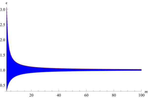
In Figure 4 we can see such behavior compared to the contribution per particle to the classical bound, .

V.3 A spin glass
Finally we consider a Hamiltonian similar to Eq. (64) for , where all the couplings are random, generated from a Gaussian probability distribution with mean and standard deviation , like a spin glass:
| (78) |
We can efficiently compute the ground state of Eq. (78) and the classical bound of the CHSH-like Bell inequality associated to it with the methods we have presented, although numerically. We expect that, when , we do not detect nonlocality, as the resulting inequality is close to the monogamous limit of Example V.2. However, if is big enough, one expects to have links with high weight surrounded with links with smaller weight; then, it may compensate to violate those links with higher weight. In Figure 6 we show the result, for spins, averaged over realizations. There is clearly a transition for which the complexity of the ground state allows or does not allow for the statistics that one obtains when performing measurements on it to be simulable locally.

V.4 An XXZ-like spin model based on Gisin’s Elegant Bell inequality
In this last example, we present an XXZ-like Hamiltonian, which is not solvable via the JW transformation. We find its ground state energy numerically, using tensor networks and DMRG [30]. In this case we find a much richer structure than in Example V.2. The Bell inequality that we associate to this Hamiltonian is a modification of Gisin’s Elegant Bell inequality [29]. Gisin’s original inequality is defined in a bipartite scenario with four dichotomic measurements with outcomes on Alice and three dichotomic measurements with outcomes on Bob:
| (79) |
and it reads . We observe that with the following observables:
| (80) |
the corresponding Bell operator becomes
| (81) |
and its ground state is , yielding an expectation value .
Let us now introduce the following modification, where is a real parameter,
| (82) |
| (83) |
where is a matrix defined as
| (84) |
The classical bound becomes
| (85) |
Now we have that the Bell operator has become
| (86) |
in either case. Its ground state energy is
| (87) |
The ground state is if and it lies in the subspace spanned by and if .
We can now construct the many-body Bell inequality in a similar fashion as in Example V.2:
| (88) |
Note that the Bell inequality has binary measurements with outcomes on the even sites and binary measurements with outcomes on the odd sites.
The dynamic programming procedure yields the following classical bound in terms of and , which is a piece-wise continous function. Due to all the cases that appear, and the complexity of the inequality, we omit the description of the local deterministic strategy. The regions are defined as follows (see Fig. 7):
| (89) |
If , , the classical bound is, on each region:
| (90) |
whereas if , the classical bound simplifies to
| (91) |
Using the measurements on the even sites and the ones on the odd sites, this yields the following XXZ-type Hamiltonian:
| (92) |
where . The ground state of Eq. (92) does not have an analytically closed form and has to be computed using DMRG. To do so, we have used the iTensor library [30]. The results are plotted in Fig. 8, where we observe quantum violations in a parameter region that does not seem to vanish as grows. We also observe a different behavior depending on the parity of , which we attribute to some sort of frustration arising in the classical optimization, especially for low values of .
VI Conclusions and outlook
In this work we have shown, on the one hand, that the ground states of some spin Hamiltonians are nonlocal. We have associated a Bell inequality to the Hamiltonian and we have computed its classical bound. We have exactly diagonalized the Hamiltonian and we have computed the quantum value of the corresponding Bell inequality. We have achieved this goal by combining two rather unexplored techniques in quantum information, which are dynamic programming and the Jordan-Wigner transformation. This has allowed us to detect the presence of nonlocal correlations. On the other hand, these tools have provided us a new way to determine the classical bound of certain classes of Bell inequalities, and look for their quantum violation under conveniently chosen observables. In the case of two dichotomic measurements, the optimization also yields the quantum bound (the maximal quantum violation) of the inequality. In the TI case, we have provided an algorithm to find the classical bound that is exponentially faster in the system size and we have obtained exact analytical solutions for the quantum value. Then, we have applied these techniques to several examples in which we reveal nonlocality: A tight TI Bell inequality with a TI Bell operator for parties, a quasi TI Bell inequality with a uniparametric quasi TI XY Hamiltonian and the ground state of a XY spin glass in some parameter region. We have also seen that for interacting models such as XXZ-like spin Hamiltonians, our method can be applied. There, we find the ground state energy numerically and we map the Hamiltonian to a modified version of Gisin’s Elegant Bell inequality. These findings open the possibility to the implementation of multipartite quantum information protocols that use nonlocality as a key resource, by using ground states of Hamiltonians that appear naturally.
We remark that the Hamiltonians and the Bell inequalities we have studied have a finite interaction range, which in the TI case makes them particularly interesting from an experimentally-friendly perspective. Note that previous Bell inequalities for quantum many-body systems with low order correlators were specially designed for a permutationally invariant (PI) symmetry [25, 26]; while being able to detect nonlocality in ground states of physical Hamiltonians such as the Lipkin-Meshkov-Glick [43, *LMG2, *LMG3] or a spin-squeezed Bose-Einstein condensate [27], the information accessible to these inequalities is bound to a de Finetti theorem [46, 47], thus becoming more compatible with that produced by a separable state as the system grows [26]. This requires to increase the number of measurements with the system size in order to close the finite-statistics loophole [27]. However, many systems of interest are not PI, but TI, and we have studied the latter in this work. In this case, a de Finetti restriction does not apply, making the detection of nonlocality more robust to experimental imperfections. Interestingly, to study the Bell inequalities proposed in [25, 26], in the classical and quantum many-body regime, one employs powerful mathematical tools (namely, convex hulls of semialgebraic sets [48] or the Schur-Weyl duality from representation theory [49], respectively), which no longer apply when the PI symmetry is broken. Here we have used other mathematical tools (dynamic programming for the classical bound and the JW transformation for the quantum value) that allowed us to solve, even exactly, the two cases with this much weaker symmetry.
Let us finalize by pointing out possible future research directions that stem from our work. Throughout this paper, we have restricted ourselves to the study of nonlocality in one-dimensional spin short-ranged Hamiltonians, as we could compute their ground state energy with exact diagonalization. One can eliminate this restriction and study short-ranged spin Hamiltonians by using a Matrix Product State (MPS) description of the state, which is a good ansatz for these systems [50]. The Bell inequalities that we would naturally associate to them would still be of the form of Eq. (8), because the interaction range would be fixed, so we could still efficiently find their classical bound. Conversely, we can eliminate the restriction on the subset of observables that we choose in Section III and the string of ’s in the middle of the string operators, thus studying purely two-body correlator inequalities like the classes derived in [38]. In such cases, powerful numerical algorithms such as DMRG [51] would be suitably tailored to perform the quantum optimization and check whether nonlocality is detected. Another interesting problem is related to the persistency of nonlocality [52]. While the tools to carry this kind of analysis in the PI case have been put forward [26], in the case of one spatial dimension we do not know yet how robust are the inequalities we have presented to particle losses. One could also generalize our results towards other directions. Since Bell inequalities with more than two inputs or outputs per party are not, in general, maximally violated by measuring qubits [53], if one would like to increase the chance to detect nonlocality with these more general classes of Bell inequalities, increasing the physical dimension of the system would be a way to obtain better results. The tools presented here could be extended by using a generalized JW transformation [54] from qudits to parafermions, although the problem becomes algebraically more involved.
We have also seen through the examples presented that there is a strong relation between Hamiltonians of physical systems and Bell inequalities that we associate to them. Whereas we naturally establish this connection in the following direction: starting from the Hamiltonian of a physical system, we assign a Bell inequality to it, one can think of this relation in a more general way, since there are many Bell inequalities that, with the appropriate observables, realize the same physical Hamiltonian. Moreover, in Example V.4, we have seen that this correspondence can be non-trivial, as the inequality does not even have the same number of measurements at every site. With the tools we have presented here, it is now possible that, given a physical one-dimensional Hamiltonian with short-range interactions, tailor the best Bell inequality that reveals the nonlocality of its ground state, as such Hamiltonian corresponds to the realization of a Bell operator of many different Bell inequalities, each with its own classical bound, which we can compute efficiently.
VII Acknowledgments
We acknowledge support of the EU Integrated Project SIQS, EU FET Proactive QUIC, Spanish MINECO (SEVERO OCHOA programme for Centres of Excellence in R&D SEV-2015-0522, National Plan Projects FOQUS FIS2013-46768, FISICATEAMO FIS2016-79508-P and QIBEQI FIS2016-80773-P), the Generalitat de Catalunya (SGR 874, SGR 875 and the CERCA programme), Fundació Privada Cellex, ERC AdG OSYRIS and CoG QITBOX, the AXA Chair in Quantum Information Science and the John Templeton Foundation. J. T. gratefully acknowledges a Max Planck - Prince of Asturias Award mobility grant and the CELLEX-ICFO-MPQ programme. G. D. L. C. acknowledges support from the Elise Richter fellowship of the FWF. R. A. acknowledges funding from the European Union’s Horizon 2020 research and innovation programme under the Marie Skłodowska-Curie grant agreement No 705109.
References
- [1] John S Bell, “On the einstein-podolsky-rosen paradox,” Physics 1, 195–200 (1964).
- [2] Arthur Fine, “Hidden variables, joint probability, and the bell inequalities,” Phys. Rev. Lett. 48, 291–295 (1982).
- [3] Nicolas Brunner, Daniel Cavalcanti, Stefano Pironio, Valerio Scarani, and Stephanie Wehner, “Bell nonlocality,” Rev. Mod. Phys. 86, 419–478 (2014).
- [4] B. Hensen, H. Bernien, A. E. Dréau, A. Reiserer, N. Kalb, M. S. Blok, J. Ruitenberg, R. F. L. Vermeulen, R. N. Schouten, C. Abellán, W. Amaya, V. Pruneri, M. W. Mitchell, M. Markham, D. J. Twitchen, D. Elkouss, S. Wehner, T. H. Taminiau, and R. Hanson, “Loophole-free bell inequality violation using electron spins separated by 1.3 kilometres,” Nature 526, 682–686 (2015).
- [5] Marissa Giustina, Marijn A. M. Versteegh, Sören Wengerowsky, Johannes Handsteiner, Armin Hochrainer, Kevin Phelan, Fabian Steinlechner, Johannes Kofler, Jan-Åke Larsson, Carlos Abellán, Waldimar Amaya, Valerio Pruneri, Morgan W. Mitchell, Jörn Beyer, Thomas Gerrits, Adriana E. Lita, Lynden K. Shalm, Sae Woo Nam, Thomas Scheidl, Rupert Ursin, Bernhard Wittmann, and Anton Zeilinger, “Significant-loophole-free test of bell’s theorem with entangled photons,” Phys. Rev. Lett. 115, 250401 (2015).
- [6] Lynden K. Shalm, Evan Meyer-Scott, Bradley G. Christensen, Peter Bierhorst, Michael A. Wayne, Martin J. Stevens, Thomas Gerrits, Scott Glancy, Deny R. Hamel, Michael S. Allman, Kevin J. Coakley, Shellee D. Dyer, Carson Hodge, Adriana E. Lita, Varun B. Verma, Camilla Lambrocco, Edward Tortorici, Alan L. Migdall, Yanbao Zhang, Daniel R. Kumor, William H. Farr, Francesco Marsili, Matthew D. Shaw, Jeffrey A. Stern, Carlos Abellán, Waldimar Amaya, Valerio Pruneri, Thomas Jennewein, Morgan W. Mitchell, Paul G. Kwiat, Joshua C. Bienfang, Richard P. Mirin, Emanuel Knill, and Sae Woo Nam, “Strong loophole-free test of local realism,” Phys. Rev. Lett. 115, 250402 (2015).
- [7] Antonio Acín, Nicolas Brunner, Nicolas Gisin, Serge Massar, Stefano Pironio, and Valerio Scarani, “Device-independent security of quantum cryptography against collective attacks,” Phys. Rev. Lett. 98, 230501 (2007).
- [8] S. Pironio, Ll. Masanes, A. Leverrier, and A. Acín, “Security of device-independent quantum key distribution in the bounded-quantum-storage model,” Phys. Rev. X 3, 031007 (2013).
- [9] Roger Colbeck, Quantum And Relativistic Protocols For Secure Multi-Party Computation, Ph.D. thesis, University of Cambridge (2006).
- [10] Roger Colbeck and Renato Renner, “Free randomness can be amplified,” Nat Phys 8, 450–453 (2012), 10.1038/nphys2300.
- [11] Rodrigo Gallego, Lluis Masanes, Gonzalo De La Torre, Chirag Dhara, Leandro Aolita, and Antonio Acín, “Full randomness from arbitrarily deterministic events,” Nature Communications 4, 2654 (2013), article.
- [12] Dominic Mayers and Andrew Yao, “Quantum cryptography with imperfect apparatus,” in Proceedings of the 39th Annual Symposium on Foundations of Computer Science, FOCS ’98 (IEEE Computer Society, Washington, DC, USA, 1998) p. 503.
- [13] I Šupić, R Augusiak, A Salavrakos, and A Acín, “Self-testing protocols based on the chained bell inequalities,” New Journal of Physics 18, 035013 (2016).
- [14] Luigi Amico, Rosario Fazio, Andreas Osterloh, and Vlatko Vedral, “Entanglement in many-body systems,” Rev. Mod. Phys. 80, 517–576 (2008).
- [15] Immanuel Bloch, Jean Dalibard, and Wilhelm Zwerger, “Many-body physics with ultracold gases,” Rev. Mod. Phys. 80, 885–964 (2008).
- [16] Olaf Mandel, Markus Greiner, Artur Widera, Tim Rom, Theodor W. Hansch, and Immanuel Bloch, “Controlled collisions for multi-particle entanglement of optically trapped atoms,” Nature 425, 937–940 (2003).
- [17] Robert McConnell, Hao Zhang, Jiazhong Hu, Senka Cuk, and Vladan Vuletic, “Entanglement with negative wigner function of almost 3,000 atoms heralded by one photon,” Nature 519, 439–442 (2015).
- [18] C. Gross, T. Zibold, E. Nicklas, J. Estève, and M. K. Oberthaler, “Nonlinear atom interferometer surpasses classical precision limit,” Nature 464, 1165–1169 (2010).
- [19] P. D. Drummond, “Violations of bell’s inequality in cooperative states,” Phys. Rev. Lett. 50, 1407–1410 (1983).
- [20] George Svetlichny, “Distinguishing three-body from two-body nonseparability by a bell-type inequality,” Phys. Rev. D 35, 3066–3069 (1987).
- [21] Marek Żukowski and Časlav Brukner, “Bell’s theorem for general n-qubit states,” Phys. Rev. Lett. 88, 210401 (2002).
- [22] R. F. Werner and M. M. Wolf, “All-multipartite bell-correlation inequalities for two dichotomic observables per site,” Phys. Rev. A 64, 032112 (2001).
- [23] Otfried Gühne, Géza Tóth, Philipp Hyllus, and Hans J. Briegel, “Bell inequalities for graph states,” Phys. Rev. Lett. 95, 120405 (2005).
- [24] László Babai, Lance Fortnow, and Carsten Lund, “Non-deterministic exponential time has two-prover interactive protocols,” computational complexity 1, 3–40 (1991).
- [25] J. Tura, R. Augusiak, A. B. Sainz, T. Vértesi, M. Lewenstein, and A. Acín, “Detecting nonlocality in many-body quantum states,” Science 344, 1256–1258 (2014a).
- [26] J. Tura, R. Augusiak, A.B. Sainz, B. Lücke, C. Klempt, M. Lewenstein, and A. Acín, “Nonlocality in many-body quantum systems detected with two-body correlators,” Annals of Physics 362, 370 – 423 (2015).
- [27] Roman Schmied, Jean-Daniel Bancal, Baptiste Allard, Matteo Fadel, Valerio Scarani, Philipp Treutlein, and Nicolas Sangouard, “Bell correlations in a bose-einstein condensate,” Science 352, 441–444 (2016).
- [28] Sophie Pelisson, Luca Pezzè, and Augusto Smerzi, “Nonlocality with ultracold atoms in a lattice,” Phys. Rev. A 93, 022115 (2016).
- [29] Nicolas Gisin, “Bell inequalities: Many questions, a few answers,” in Quantum Reality, Relativistic Causality, and Closing the Epistemic Circle: Essays in Honour of Abner Shimony (Springer Netherlands, Dordrecht, 2009) pp. 125–138.
- [30] “Itensor - intelligent tensor library,” http://itensor.org.
- [31] Norbert Schuch and J. Ignacio Cirac, “Matrix product state and mean-field solutions for one-dimensional systems can be found efficiently,” Phys. Rev. A 82, 012314 (2010).
- [32] David Avis, Hiroshi Imai, Tsuyoshi Ito, and Yuuya Sasaki, “Deriving tight bell inequalities for 2 parties with many 2-valued observables from facets of cut polytopes,” (2004), arXiv:quant-ph/0404014 .
- [33] P. Jordan and E. Wigner, “Über das Paulische Äquivalenzverbot,” Zeitschrift fur Physik 47, 631–651 (1928).
- [34] Michael A Nielsen, “The fermionic canonical commutation relations and the jordan-wigner transform,” School of Physical Sciences The University of Queensland (2005).
- [35] Mari-Carmen Bañuls, J. Ignacio Cirac, and Michael M. Wolf, “Entanglement in fermionic systems,” Phys. Rev. A 76, 022311 (2007).
- [36] M. A. de Gosson, Symplectic Geometry and Quantum Mechanics (Springer Science & Business Media, 2006) Chap. 8.
- [37] Benjamin Toner and Frank Verstraete, “Monogamy of bell correlations and tsirelson’s bound,” (2006), arXiv:quant-ph/0611001 .
- [38] J Tura, A B Sainz, T Vértesi, A Acín, M Lewenstein, and R Augusiak, “Translationally invariant multipartite bell inequalities involving only two-body correlators,” Journal of Physics A: Mathematical and Theoretical 47, 424024 (2014b).
- [39] Samuel L Braunstein and Carlton M Caves, “Wringing out better bell inequalities,” Annals of Physics 202, 22 – 56 (1990).
- [40] John F. Clauser, Michael A. Horne, Abner Shimony, and Richard A. Holt, “Proposed experiment to test local hidden-variable theories,” Phys. Rev. Lett. 23, 880–884 (1969).
- [41] Ravishankar Ramanathan and Paweł Horodecki, “Strong monogamies of no-signaling violations for bipartite correlation bell inequalities,” Phys. Rev. Lett. 113, 210403 (2014).
- [42] R. Augusiak, M. Demianowicz, M. Pawłowski, J. Tura, and A. Acín, “Elemental and tight monogamy relations in nonsignaling theories,” Phys. Rev. A 90, 052323 (2014).
- [43] H.J. Lipkin, N. Meshkov, and A.J. Glick, “Validity of many-body approximation methods for a solvable model: (i). exact solutions and perturbation theory,” Nuclear Physics 62, 188 – 198 (1965).
- [44] N. Meshkov, A.J. Glick, and H.J. Lipkin, “Validity of many-body approximation methods for a solvable model: (ii). linearization procedures,” Nuclear Physics 62, 199 – 210 (1965).
- [45] A.J. Glick, H.J. Lipkin, and N. Meshkov, “Validity of many-body approximation methods for a solvable model: (iii). diagram summations,” Nuclear Physics 62, 211 – 224 (1965).
- [46] Matthias Christandl, Robert König, Graeme Mitchison, and Renato Renner, “One-and-a-half quantum de finetti theorems,” Communications in Mathematical Physics 273, 473–498 (2007).
- [47] Fernando G.S.L. Brandao and Aram W. Harrow, “Quantum de finetti theorems under local measurements with applications,” in Proceedings of the Forty-fifth Annual ACM Symposium on Theory of Computing, STOC ’13 (ACM, New York, NY, USA, 2013) pp. 861–870.
- [48] P. A. Parrilo G. Blekherman and R. R. Thomas (Editors), in Semidefinite Optimization and Convex Algebraic Geometry (2012).
- [49] Roe Goodman and Nolan R Wallach, Representations and invariants of the classical groups, Vol. 68 (Cambridge University Press, 2000).
- [50] F. Verstraete, V. Murg, and J.I. Cirac, “Matrix product states, projected entangled pair states, and variational renormalization group methods for quantum spin systems,” Advances in Physics 57, 143–224 (2008).
- [51] Román Orús, “A practical introduction to tensor networks: Matrix product states and projected entangled pair states,” Annals of Physics 349, 117 – 158 (2014).
- [52] Nicolas Brunner and Tamás Vértesi, “Persistency of entanglement and nonlocality in multipartite quantum systems,” Phys. Rev. A 86, 042113 (2012).
- [53] Daniel Collins, Nicolas Gisin, Noah Linden, Serge Massar, and Sandu Popescu, “Bell inequalities for arbitrarily high-dimensional systems,” Phys. Rev. Lett. 88, 040404 (2002).
- [54] Wei Li, Shuo Yang, Hong-Hao Tu, and Meng Cheng, “Criticality in translation-invariant parafermion chains,” Phys. Rev. B 91, 115133 (2015).
- [55] Jean Gallier, Geometric methods and applications: for computer science and engineering, Vol. 38 (Springer Science & Business Media, 2011).
- [56] K. Fukuda, “cdd/cdd+ reference manual,” https://www.inf.ethz.ch/personal/fukudak/cdd_home/ (2015).
Appendix A The parity operator
Here we prove Eq. (31). Let be an orthogonal transformation relating the sets of Majorana fermions and , as in Eq. (23). Recall that the Cartan-Dieudonné Theorem [55] states that every orthogonal transformation decomposes as a product of a number of reflections (at most, ). Hence, it suffices to show that a reflection flips the parity operator; i.e., our aim is to show that
| (93) |
whenever is a reflection. Recall that any reflection with respect to a hyperplane with normal vector can be written as . We will denote the LHS of Eq. (93) and the RHS of Eq. (93) .
The CARs (20) ensure that
| (94) |
and
| (95) |
Hence, the operators and respectively share an eigenbasis and split the Fock space into even and odd subspaces with respect to the parity operator defined in Eq. (27).
We prove in Theorem 1 that this partition of the Fock space does not change under orthogonal transformations. Moreover, if , the subspaces are just swapped. Theorem 1 is supported on Lemma 2, which proves that reflections swap the eigenspaces, and Lemma 1 contains the technical steps to prove Lemma 2. Hence, Eq. (93) follows and, because every orthogonal transformation is a product of a number of reflections, we obtain Eq. (31).
Lemma 1.
Consider a reflection , where is a normalized vector. Let us define the following quantities:
| (96) |
Then, the identities
| (97) |
and
| (98) |
hold.
Proof.
To prove Eq. (97), we can split the sum into the indices for which and the indices for which .
In the first case, since the CARs (20) imply that we have a term which contributes , because is normalized.
In order to prove Eq. (98), we begin by noting that
| (100) |
We can now split the sum (98) into the parts where and .
Lemma 2.
Let be a reflection. Then,
| (102) |
Proof.
By hypothesis, , where is the Kronecker delta function. Let us now see how the operator relates to the Majorana fermions.
By definition (cf. Eq. (23)), we can write
Lemma 1 allows us to conclude
| (103) |
showing that a reflexion flips the parity of the vacuum: The occupation number operator, in terms of the operators has opposite parity than the occupation number operator in terms of the operators:
| (104) |
∎
Theorem 1.
Let . Let be the Fock space of Dirac Fermions. The operator splits into even and odd subspaces: . Similarly, splits as . Then, either (if ) or (if ).
Proof.
Recall that the expectation value of the operator is the occupation number of the -th mode, denoted . Then, a basis of the Fock space of fermionic Dirac modes can be defined as
| (105) |
where the product is written from left to right. Note that can only be or , due to (17). The CARs (17) further imply that whenever ( and differ only in its -th index) and whenever .
Let be an eigenvector of of eigenvalue . We can assume, without loss of generality, that is a basis element of the Fock space, with . By noting that can be expressed as
we see that the only operators which appear are products of or with or . Hence, they either annihilate or they add , or to its particle number; always conserving its parity. This leaves us with a linear combination of vectors that live in the same subspace , so it remains on . The same argument applies to .
Hence, the subspaces and of the operator are invariant under orthogonal transformations of the Majorana fermions. However, under , they might change its parity. Because of linearity and Eq. (105), it suffices to prove that is an eigenstate of , as it stems from Lemma 2. If its eigenvalue is , then ; if it is , then . ∎
Appendix B The PBC to OBC reduction
In this appendix we describe the reduction of the optimization problem of finding the classical bound in a Bell inequality with PBC to the optimization problem of finding the classical bound for a Bell inequality with OBC in one dimension.
For the sake of clarity, we first describe the procedure for inequalities with an arbitrary interaction range , but without the chain of observables in the middle of the string operators (cf. Eq. (7)), so that the inequalities strictly contain one or two-body correlators. We pick consecutive parties. Without loss of generality, we can assume them to be labelled from to . To these parties we assign one of the possible deterministic local strategies. Let be a pair of parties. There are three cases to consider:
- •
If and are between and , any correlator between parties and has now a definite value.
- •
If either or , but not both are between and , only one side of the correlator has a definite value. Because the classical bound is computed on a deterministic local strategy, the value of the correlator factorizes as the product of the local values assigned by the strategy we are considering. Hence, these correlators can be effectively moved outside of the interval by updating the one-body term of the party outside that interval.
- •
In any other case, the correlator remains the same.
In Figure 9 a) and Figure 9 b) we illustrate this procedure for an example with . The first case is illustrated in blue; the second is illustrated in red and the last one is illustrated in black.
Finally, if we have an inequality of the form of Eq. (7), the intermediate terms should also be taken into account when performing this procedure. In order to move to the -body terms the -body terms, now an extra number of observables should also be chosen in advance for those parties at distance to the set (but only the -th observable; it is not necessary to fix the rest). For instance, in the example of Figure 9 c), one would have to specify the value of and . Observe that if , then in the OBC problem, some of the values closest to the boundary become fixed ( of them). This has to be taken into account when performing the dynamical programming, as one should only explore those configurations compatible with the boundary conditions imposed by the PBC problem with the deterministic local strategy that we have chosen to make the reduction.
Appendix C Quantum optimization of translationally invariant Bell inequalities
In this appendix we discuss the quantum optimization for the translationally invariant (TI) case (i.e., when the Bell inequality is TI and the same set of measurements are performed at each site, thus leading to a TI Bell operator). We begin by observing that there are two cases to consider, depending on the choice of the parity of the fermion number: If , the matrix (cf. Eq. (18)) is block-circulant: , where the party indices are taken modulo . We can then define to be the block of whose entries are given by . If , the matrix is no longer block circulant because the blocks of that correspond to interactions that cross the origin carry a minus sign (these blocks are located on the top-right diagonals and bottom-left diagonals of ). In this latter case, it is convenient to construct
| (106) |
where , which is now circulant. Note that half of the spectrum of are zeroes and the other half coincides with the spectrum of . For instance, for the case of nearest neighbour interactions (), parties and , takes the block-form
| (107) |
It is then clear that is block-circulant.
Circulant matrices can be diagonalized via a Discrete Fourier Transform (DFT). The DFT matrix is unitary in general, but we want to use an orthogonal transformation instead, so that we can transform Majorana fermions into Majorana fermions and obtain Eq. (21). Let us consider the following Real DFT (RDFT) matrix of order :
| (108) |
It is easy to see that and , so is orthogonal. In the following, we are going to use the fact that for any , .
Let us now, with the aid of the orthogonal transformation , study which invariant subspaces acts upon. If , then we compute ; if then we calculate . Note that acts on the two Majorana modes asociated to one site.
On the one hand, if , a direct calculation of shows that
| (109) |
where the last subspace only appears if is even and each is a block defined as
| (110) |
On the other hand, if , one similarly proves that :
| (111) |
where the last subspace only appears if is odd, and each is a block defined as
| (112) |
We can further simplify these expressions by noting that is block-wise equivalent to . This implies that the blocks in Eqs. (109) and (111) are already brought to the Williamson form:
| (113) |
and
| (114) |
We then define the quantity
| (115) |
which corresponds to the Williamson eigenvalue(s) for the blocks.
To bring to a Williamson form, it remains to bring the blocks and to a Williamson form. To this end, let us start by defining and
| (116) | |||||
| (117) | |||||
| (118) | |||||
| (119) |
Let us notice that the blocks (or ) take the following form:
| (120) |
Now we are ready to find an orthogonal transformation that brings or to a Williamson form, which we state in the following lemma:
Lemma 3.
For every (or ) of the form (120), there exists an orthogonal transformation that brings it to a Williamson form
| (121) |
Its two Williamson eigenvalues , are given by
| (122) |
where and ranges from to . Furthermore, this orthogonal transformation always satisfies .
Proof.
The choice of is not unique in general. Here we are going to construct as the product of three matrices. Since is fixed, we are going to skip explicitly stating the subindex throughout the proof. We construct as , where and are diagonal matrices whose entries are defined by:
| (123) |
and
| (124) |
where . The matrix in the middle is not diagonal, and in its most general form, can depend on two real parameters, which we denote and . We have that the entries of are given by
| (125) |
where
and
We can now show that is indeed an orthogonal transformation with determinant , since , and the determinant of is independent of both and , and it is . The multiplication of these three terms gives the result . Hence, one can pick convenient values for and in order to show that already has a Williamson form (121) simply by matrix multiplication. ∎
Appendix D Tight translationally invariant inequalities
In this appendix we provide a list of tight optimal TI Bell inequalities (53) for that are violated when performing the same set of measurements on each party, which are of the form
Note that, since
| (126) |
where is a unitary transformation of the form , the maximal quantum violation of a TI Bell inequality with the above measurements only depends on , as there always exists a unitary that brings to by performing a rotation in the plane [26]. Hence, there is no loss of generality in assuming .
For it is still computationally feasible to find all the facets of the polytope of local correlations projected onto the space of the correlators appearing in Eq. (53). To achieve this goal, we construct all the vertices of the local polytope of correlations for parties, measurements and outcomes, which are in total, and we project them to the space of translationally invariant correlators that appear in (53), following the same procedure of [38]. With linear programming, we can remove all the projected vertices that are a convex combination of other projected vertices. Then, we can use an algorithm such as CDD [56] to compute the convex hull of the extremal projected vertices and obtain a minimal description of it in terms of facets. We call these facets tight Bell inequalities. We summarize these findings in Table 1:
| Number of facets | Number of vertices | |
|---|---|---|
| 3 | 166 | 72 |
| 4 | 5628 | 204 |
| 5 | 46804 | 1148 |
| 6 | 20268 | 1816 |
| 7 | 175444 | 6064 |
| 8 | 29290 | 4044 |
Following the same procedure as in Example V.1, we find the inequalities that are violated, which we classify in the Table 2.
Note that by renaming the outcomes of the measurements, the labels of the measurements or the labels of the parties, one can obtain other inequalities that are not listed in the table; however, these relabellings do not change the properties we are interested in, such as the classical bound or its quantum violation, so we consider them to be equivalent and we include only one representative for each equivalence class.
From the values of Table 2, we see that approaches zero as grows. Similar to what was found in [38], numerics suggest that, for translationally invariant Bell inequalities, there is a trade-off between and . In [38], the maximal for was , whereas here for we did not find any violation beyond . Furthermore, for there are no translationally invariant Bell inequalities of the form (53) that are violated by performing the same qubit measurements at each site. One may still perform different qubit measurements on each site and be able to maximally violate the inequality, as it was proven in [37]; however to achieve the same violation with the same set of measurements at each site, one may then need to increase the dimension of the state and use POVMs [38].
Interestingly, we also note that the highest ratio is obtained for . This is not surprising, as for our inequalities contain full-body correlators (see Table 2). However, for , the first class achieves a much higher violation than the others. This is because the inequality consists of a sum of CHSH-like inequalities between parties and and between parties and :
| (127) |
The minimum over quantum values that can be achieved is , so that . This inequality can be generalized to any even number of parties at the price of increasing the interaction range . By picking one can always pair party with party into a CHSH-like link while maintaining for any even . However, let us remark that for the scope of this work, we are interested in studying the nonlocality of ground states of local Hamiltonians (i.e., with a fixed ).
Appendix E The orthogonal transformation for Majorana fermions
We consider an antisymmetric matrix of size . If we want to decompose it as , where is a orthogonal matrix and has the form (21), we can in the majority of situations, use the Spectral Theorem to find : The matrix is symmetric, so it diagonalizes as , with a diagonal matrix with entries , appearing with multiplicity for each , and the columns of forming an orthonormal basis. If all the are different, then one can safely conclude that , because if is antisymmetric, then has to be of the form (46). Hence, one can say that is unique (up to permutations that determine the order and the signs of ).
However, if has a multiplicity greater than , this need no longer be the case, as the found via the Spectral Theorem is no longer unique (one can perform an arbitrary orthogonal transformation in each eigenspace). Note that this pathologic case is of interest to our problem, as for tight Bell inequalities with the optimal set of measurements, it is common to find ’s with the same value (for instance, in Example V.1). There are two ways to circumvent this problem: one is to add some noise to such that all the ’s can be considered different; however we lose precision in the solution and add numerical instability. The other way is described below.
Let be a nonzero Williamson eigenvalue of with multiplicity . Then, has a block, denoted , that satisfies
| (128) |
Thus, any orthogonal transformation acting on leaves invariant, but not necessarily in the form (21). Let be a unit vector in the eigenspace (picked from the corresponding columns of ) and let be another unit vector. Then, we observe that because of Eq. (128). Now, by picking another unit vector from , we find with the same procedure. We repeat this process times. By multiplying by the orthogonal transformation given by the vectors we obtain the right transformation bringing to the form (21).
| QV | ||||||||||||
| 3 | -2 | 1 | -1 | 1 | 1 | -1 | -1 | 1 | -1 | 6 | -2.9282032303 | |
| 3 | 0 | 1 | -1 | 3 | -3 | 1 | 1 | 1 | 1 | 12 | -2.5830052443 | |
| 3 | 2 | -1 | 1 | 1 | 1 | -1 | 1 | 1 | 1 | 6 | -2.5830052443 | |
| 4 | 0 | 0 | 0 | 0 | 0 | 1 | -2 | 0 | -1 | 8 | -3.313708499 | |
| 4 | -2 | 4 | 2 | 2 | 0 | 5 | -3 | 1 | -1 | 32 | -0.5471047512 | |
| 4 | 0 | 2 | 2 | 2 | 2 | 5 | -5 | 1 | -1 | 32 | -0.5115214246 | |
| 4 | -1 | 2 | 5 | 5 | 6 | -2 | -10 | 2 | 11 | 72 | -0.4999666746 | |
| 4 | -1 | -2 | -3 | -3 | -4 | -7 | 7 | -1 | 2 | 48 | -0.4670552431 | |
| 4 | 2 | 0 | -2 | -2 | -4 | 3 | 1 | -3 | -3 | 32 | -0.218521874 | |
| 5 | 0 | 1 | 1 | -1 | -1 | 1 | -1 | 1 | -1 | 12 | -0.3107341487 | |
| 8 | 0 | 2 | -2 | 2 | -2 | -1 | -1 | 1 | 1 | 32 | -0.2187 |