Zeros and Amoebas of Partition Functions

The partition function is a key object in various branches of physics. In statistical physics, due to the relation with the free energy $F=-k_{B}T\ln\mathcal{Z}$, all basic thermodynamic characteristics of a macroscopic system are encoded in the partition function

where $\{E_{n}\}$ is the energy spectrum, $g_{n}$ is the degeneracy of the $n$-th state, $T$ is the temperature and $k_{B}$ is the Boltzmann constant (see e.g. [1, 2]). In equilibrium $\mathcal{Z}$ is finite and positive, otherwise it is an indication of instability of the system.

Zeros of the partition function as a function of physical parameters (temperature, magnetic field etc.) are of particular interest since at such points the free energy becomes singular and, hence, the system changes of state, e.g. exhibits a phase transition [1, 2]. Since the seminal papers of Lee and Yang [3, 4] it is known that for usual systems (with finite and positive $g_{n}$ and real $E_{n}$) zeros of the partition functions lie in the complex plane (see e.g. [2, 5, 6, 7, 8, 9, 10, 11, 12, 13, 14]). These results have led to the intensive study of the partition function’s zero sets and associated phase transitions in the complex plane of physical parameters for a number of models in statistical physics, including those subject to quantum dynamics (see e.g. [15, 16, 17, 18]).

Study of unstable or metastable states is another branch of statistical physics where complex-valued partition functions naturally arise [19, 20]. Formally, for an unstable state the energy $E_{n}$ is complex $E_{n}=E_{n,0}+\mathrm{i}\Delta E_{n}$ with width $\Delta E_{n}$ and, hence, the partition function is complex-valued too. Wide classes of macroscopic systems like spin-glasses and other geometrically or dynamically frustrated systems have such peculiarity (see e.g. [21, 22, 23, 24, 25, 26, 27]).

In all these cases the situation when partition function’s zeros are real is of the greatest interest. The study of properties of macroscopic systems, in particular, structure of equilibrium and unstable domains, is simplified if the partition function is real-valued for all values of parameters. Such situation is realisable, for example, for spin-glasses and frustrated systems with different temperatures $T_{n}$ of microsystems (microbasins) if the widths $\Delta E_{n}$ of energy levels obey the condition ${\displaystyle\frac{\Delta E_{n}}{k_{B}T_{n}}=\ell_{n}\pi}$, $n=1,2,3,\dots$ where $\ell_{n}$ are integers. Terms with odd $\ell_{n}$ acquire the factor $-1$ and, hence, the partition function $\mathcal{Z}$ is of the form (1.1) and real-valued, but with $g_{n}$ assuming both positive and negative values. Negative degeneracies of energy levels can be interpreted as the contribution from sort of holes in spectrum. Formally, negativity of $g_{n}$ is closely connected with the concepts of negative probability and negative membership functions widely discussed in literature (see e.g. [28, 29, 30] and references therein).

This paper is devoted to the study of partition functions of such a type, more precisely, those of the form

where factors $g_{\alpha}$ take values $1$ or $-1$, $x_{1},\dots,x_{n}$ are real variables and $f_{\alpha}(\boldsymbol{x})$ are linear real-valued functions. Main attention is paid to an analysis of the singular sector $\mathcal{Z}_{\mathrm{sing}}$ (locus of zeros) of the partition function (1.2), its stratification and structure of stability ($\mathcal{Z}(\boldsymbol{g};\boldsymbol{x})>0$) and zero confinement domains in the space $\mathbb{R}^{n}$ of parameters $(x_{1},\dots,x_{n})$.

Singular sector $\mathcal{Z}_{\mathrm{sing}}$ admits a natural stratification

the stratum $\mathcal{Z}_{\mathrm{sing},k}$ is composed by all hypersurfaces given by ${\displaystyle\binom{N}{k}}$ equations

where $(\mathcal{I},[N]\backslash\mathcal{I})$ is any $2$-partition of the set $[N]:=\{1,2,\dots,N\}$ with cardinality $\#\mathcal{I}=k$. These hypersurfaces for the $k$-stratum are contained in a certain domain in $\mathbb{R}^{n}$ refered as the zero confinement domain $ZCD_{k}$. This domain is divided by hypersurfaces (1.4) into a number of subdomains $ZCD_{k;\delta}$ at which each of the $\binom{N}{k}$ functions $\mathcal{Z}_{k}$ in (1.4) is positive or negative. This allows to associate with each of these subdomains a set of $\binom{N}{k}$ number $1$ or $-1$ that can be viewed as the state of the system of $\binom{N}{k}$ “spins” which take values $1$ or $-1$.

The domain $\mathcal{D}_{k+}$, where all functions (1.4) are positive, is the stability (equilibrium) domain. The union $\mathcal{A}_{k}:=\mathcal{D}_{k+}\cup ZCD_{k}$ is called the statistical $k$-amoeba. A $k$-statistical amoeba is composed by the stable nucleus $\mathcal{D}_{k+}$ and intermittent shell $ZCD_{k}$ with varying degree of instability (number of signs $-1$). The complement $\mathcal{D}_{k-}$ of the $k$-amoeba in $\mathbb{R}^{n}$ is the domain with maximum number of signs $-1$, i.e. the domain of maximal instability.

The domains $\mathcal{D}_{k+}$, $ZCD_{k}$ and statistical $k$-amoebas exhibit a simple inclusion property, for instance, $\mathcal{D}_{k+}\supseteq\mathcal{D}_{\hat{k}+}$ and $\mathcal{A}_{k}\supseteq\mathcal{A}_{\hat{k}}$ if ${\displaystyle 1\leq k<\hat{k}<\frac{N}{2}}$.

Statistical $1$-amoebas $\mathcal{A}_{1}$ coincide with the so-called non-lopsided amoebas $\mathcal{LA}$ introduced in algebraic geometry [31]. Analogs of higher statistical $k$-amoebas ($k\geq 2$) seem to be not studied in algebraic geometry.

Tropical limits of statistical $k$-amoebas are considered. It is shown that all $k$-amoebas collapse into the same set of piecewise hyperplanes in $\mathbb{R}^{n}$ coinciding with that of tropical limit of $\mathcal{A}_{1}$.

It should be noted that partition functions depending on several variables (multidimensional energy spectrum or several Hamiltonians) have been considered in [32], [33] and [34]. However these papers have addressed only the case (1.2) with all positive factors $g_{\alpha}$.

In a completely different setting zeros of superpositions of the form (1.2) ($\tau$-functions) with positive and negative factors $g_{\alpha}$ and very particular linear functions $f_{\alpha}$ arise within an analysis of singular solutions of integrable equations (see e.g. [35], [36]).

The paper is organized as follows. General definitions of strata of the singular sector and some concrete examples for the first stratum $\mathcal{Z}_{\mathrm{sing},1}$ are given in section 2. Higher strata and properties of zero loci hypersurfaces are considered in section 3. Section 4 is devoted to the study of some general properties of equilibrium and zero confinement domains. Statistical amoebas and their relation to algebraic amoebas are discussed in section 5. Next section 6 is devoted to an analysis of the structure and properties of $ZCD_{k}$ domains and associated statistical systems of “spins”. Tropical limits of statistical amoebas are considered in section 7. In conclusion some peculiarities of partition function (1.2) with nonlinear functions $f_{\alpha}$ are noted.

So we will consider the family of partition functions of the form

where ${\displaystyle f_{\alpha}(\boldsymbol{x})=b_{\alpha}+\sum_{i=1}^{n}a_{\alpha i}x_{i}}$, all variables $g_{\alpha}$, $x_{i}$ and all functions $f_{\alpha}$ are real. Since $g_{\alpha}e^{b_{\alpha}}=\text{sign}(g_{\alpha})\cdot e^{\log|g_{\alpha}|+b_{\alpha}}$ one can consider only the case $g_{\alpha}\in\{+1,-1\}$.

The space $V$ of parameters $g_{1},\dots,g_{N},x_{1},\dots,x_{n}$ admits the stratification

where $V_{\alpha}$ is the union of subspaces of $V$ with $\alpha$ many negative $g_{\beta}$. For instance, ${\displaystyle V_{2}=\bigcup_{1\leq\alpha<\beta\leq N,}V_{2,\{\alpha\beta\}}}$ where $\displaystyle V_{2,\{\alpha\beta\}}=\left\{(g_{1},\dots,g_{N};x_{1},\dots,x_{n}):\,g_{\alpha}=g_{\beta}=-1,\right.$
$\displaystyle\left.\gamma\neq\alpha,\beta\Rightarrow g_{\gamma}>0\right\}$, $\alpha\neq\beta$, $\alpha,\beta=1,\dots,N$. Inversion $P$ of all $g_{\alpha}$: $Pg_{\alpha}=-g_{\alpha}$, $\alpha=1,\dots N$, acts on strata $V_{\alpha}$ as $PV_{\alpha}=V_{N-\alpha}$.

Accordingly, singular sector $\mathcal{Z}_{\mathrm{sing}}$ of partition function also admits the stratification

where $\mathcal{Z}_{\mathrm{sing},k}$ are subspaces of $V_{k}$ for which $\displaystyle\mathcal{Z}|_{V_{k}}=0$. Subspaces $V_{0}$ and $V_{N}$ are obviously regular and connected by inversion $P$. First singular stratum $\mathcal{Z}_{\mathrm{sing},1}$ is the union of the $N$ hypersurfaces defined by the equations

with $g_{\alpha(\alpha)}=-1$ and $g_{\alpha(\beta)}=1$, $\beta\neq\alpha$. Geometric characteristics of such hypersurfaces have been studied in the paper [37]. Cases of linear functions $f_{\alpha}(\boldsymbol{x})$ were referred in [37] as ideal statistical hypersurfaces. General statistical hypersurfaces considered in [37] were associated with nonlinear functions $f_{\alpha}$ while super-ideal case corresponds to $N=n$ and $f_{\alpha}(\boldsymbol{x})\equiv x_{\alpha}$.

Generically the stratum $\mathcal{Z}_{\mathrm{sing},1}$ can be composed by $N$ hypersurfaces. In addition, it is easy to see that hypersurfaces given by $\mathcal{Z}_{1}(\{\alpha\};\boldsymbol{x})=0$ with different $\alpha$ do not intersect at finite values of $x_{1},\dots,x_{n}$ and $N\geq 3$. Indeed, if there exists $\alpha\neq\beta$ such that $\{\boldsymbol{x}:\mathcal{Z}_{1}(\{\alpha\};\boldsymbol{x})=0\}\cap\{\boldsymbol{x}:\mathcal{Z}_{1}(\{\beta\};\boldsymbol{x})=0\}$ is not empty, then there exists $\boldsymbol{x}_{0}$ in $\mathbb{R}^{n}$ such that ${\displaystyle e^{f_{\beta}(\boldsymbol{x}_{0})}-e^{f_{\alpha}(\boldsymbol{x}_{0})}=\sum_{\gamma\notin\{\alpha,\beta\}}e^{f_{\gamma}(\boldsymbol{x}_{0})}=e^{f_{\alpha}(\boldsymbol{x}_{0})}-e^{f_{\beta}(\boldsymbol{x}_{0})}}$, that is $f_{\beta}(\boldsymbol{x}_{0})=f_{\alpha}(\boldsymbol{x}_{0})$, so one has ${\displaystyle\sum_{\gamma\neq\alpha,\beta}e^{f_{\gamma}(\boldsymbol{x}_{0})}=0}$ which is impossible if $N\geq 3$.

The form of hypersurfaces which compose the sector $\mathcal{Z}_{\mathrm{sing},k}$ depends on $N$, $n$ and the choice of functions $f_{\alpha}(\boldsymbol{x})$. At the simplest case of $n=1$ the stratum $\mathcal{Z}_{\mathrm{sing},1}$ is composed, in general, by at most $N$ points defined by the equations

with $g_{\alpha(\alpha)}=-1$ and $g_{\alpha(\beta)}=1$, $\beta\neq\alpha$. In the case $N=2$ the sector $\mathcal{Z}_{\mathrm{sing},1}$ contains only one hypersurface defined by the equation

It is the hyperplane in $\mathbb{R}^{n}$ given by the equation

For $N\geq 3$ and $n=2$ one has a family of curves on the plane $(x_{1},x_{2})=:(x,y)$. For example, at the choice $f_{1}\equiv 0$, $f_{2}\equiv x$, $f_{3}\equiv y$ the sector $\mathcal{Z}_{\mathrm{sing},1}$ is composed by three curves shown in figure 1(a) (see also [46])

where the curves $1$, $2$ and $3$ are given by the equations

Note that at $|x|,|y|\rightarrow\infty$ the curves $1$ and $2$ tend to the ray $x=0$, $y<0$, the curves $2$ and $3$ tend to the ray $x=y$, $x>0$ while the curves $3$ and $1$ tend to the ray $y=0$, $x<0$. An example with a different homotopy and a bounded closed component (curve $4$) is given by choice $f_{1}\equiv 0$, $f_{2}\equiv 3x$, $f_{3}\equiv 3y$, $f_{4}\equiv x+y+\ln 6$ and it is shown in figure 1(b).

The stratum $\mathcal{Z}_{\mathrm{sing},1}$ at $n=2$ is composed by at most $N$ curves. For particular choice of functions $f_{\alpha}(\boldsymbol{x})$ this number can be smaller than $N$ when some equations in (2.4) define the empty set. To illustrate this let us consider the following examples with $n=2$: if one chooses

then one gets $N$ curves by symmetry. For instance, at $N=6$ one gets $6$ curves presented in figure 2(a). If, instead, one takes

then for all $2\leq\gamma\leq N-1$ the corresponding locus is empty, i.e. $\{\mathcal{Z}_{1}(\{\gamma\})=0\}=\emptyset$. Indeed, if $x\leq y$ then $e^{(\gamma-1)\cdot x}\leq e^{(\gamma-1)\cdot y}$ thus ${\displaystyle e^{f_{\gamma}(x,y)}\leq e^{f_{1}(x,y)}<\sum_{\beta\neq\gamma}e^{f_{\beta}(x,y)}}$. Similarly, If $y\leq x$ then ${\displaystyle e^{f_{\gamma}(x,y)}\leq e^{f_{N}(x,y)}<\sum_{\beta\neq\gamma}e^{f_{\beta}(x,y)}}$. The only two visible curves are given by $\mathcal{Z}_{1}(\{1\};x,y)=0$ and $\mathcal{Z}_{1}(\{N\};x,y)=0$: they are straight lines with slope $1$ passing through $(\pm\ln\chi,0)$ respectively, where $\chi>0$ is uniquely defined by $\displaystyle-1+\sum_{\alpha=1}^{5}\chi^{\alpha}=0$. See figure 2(b) for the case at $N=6$.

One has an intermediate case at $f_{1}(x,y)\equiv 0,$ $f_{2}(x,y)\equiv 3x$, $f_{3}(x,y)\equiv 3y$, $f_{4}(x,y)\equiv x+y+\ln 6$, $f_{5}(x,y)\equiv 2x+y+\ln 11$, $f_{6}(x,y)\equiv x+3y+\ln 4$. The stratum $\mathcal{Z}_{\mathrm{sing},1}$ is composed by $5$ curves given in figure 3.

One can check directly that the set of solutions of the equation

is empty. Indeed, if $\mathcal{Z}_{1}(\{4\};x,y)=0$ then $x+y+\ln 6>2x+y+\ln 11$, that is $x<\ln 6-\ln 11<0$. From the arithmetic-geometric means inequality one gets ${\displaystyle\frac{1}{2}+\frac{1}{2}+11\cdot e^{2x+y}+4\cdot e^{x+3y}\geq}$ ${\displaystyle 4\left[\frac{1}{2}\cdot\frac{1}{2}\cdot(11\cdot e^{2x+y})\cdot(4\cdot e^{x+3y})\right]^{\frac{1}{4}}=4\cdot 11^{\frac{1}{4}}\cdot e^{\frac{3x+4y}{4}}}$. But $4\cdot 11^{\frac{1}{4}}>6$ and $x<0$, hence ${\displaystyle e^{\frac{3x+4y}{4}}>e^{x+y}}$ and $\displaystyle 1+11\cdot e^{2x+y}+4\cdot e^{x+3y}\geq$ $\displaystyle 4\cdot 11^{\frac{1}{4}}\cdot e^{\frac{3x+4y}{4}}>4\cdot 11^{\frac{1}{4}}\cdot e^{x+y}>6\cdot e^{x+y}$. In particular, $\mathcal{Z}_{1}(\{4\};x,y)$ is always positive.

At $N=3$, $n=3$ and $f_{1}\equiv x$, $f_{3}\equiv y$, $f_{4}\equiv z$ ($x_{1}=x$, $x_{2}=y$, $x_{3}=z$) the stratum $\mathcal{Z}_{\mathrm{sing},1}$ contains $3$ super-ideal statistical surfaces defined by the equations

and given in figure 4.

Induced metric $g_{ik}$, Gauss curvature $K$ and mean curvature $\Omega$ of the surface given by the equation $\mathcal{Z}_{1}(\{1\})=0$ are (with $y$ and $z$ as local coordinates) [37]

where probability ${\displaystyle w_{1}=\frac{e^{y}}{e^{y}+e^{z}}}$, ${\displaystyle w_{2}=\frac{e^{z}}{e^{y}+e^{z}}}$ and ${\displaystyle T_{l}=w_{1}^{l}+w_{2}^{l}}$, $l=2,3$. For surface given by the equation $\mathcal{Z}_{1}(\{2\})=0$ and $\mathcal{Z}_{1}(\{3\})=0$ one has similar results with substitution $x\leftrightarrows y$ and $x\leftrightarrows z$, respectively. At large $x$, $y$, $z$ surfaces $1$ and $2$ tend to the half-plane $x=y$, $z<0$, surfaces $1$ and $3$ tend to the half-plane $x=z$, $y<0$ and surfaces $2$ and $3$ tend to the half-plane $y=z$, $x<0$.

Last example is presented in figure 5 and corresponds to $N=6$ and $n=3$ with $f_{1}(x,y,z)=0$, $f_{2}(x,y,z)=3x$, $f_{3}(x,y,z)=3y$, $\,f_{4}(x,y,z)=2x+z+\log 6$, $f_{5}(x,y,z)=2x+y+z+\log 11$, $f_{6}(x,y,z)=3y+z+\log 4$.

Higher strata $\mathcal{Z}_{\mathrm{sing},k}$ have rather complicated structure. For instance, for $N=6,$ $n=2$ and functions $f_{\alpha}(x,y)$ given, as in figure 3, by $f_{1}(x,y)\equiv 0,$ $f_{2}(x,y)\equiv 3x$, $f_{3}(x,y)\equiv 3y$, $f_{4}(x,y)\equiv x+y+\ln 6$, $f_{5}(x,y)\equiv 2x+y+\ln 11$, $f_{6}(x,y)\equiv x+3y+\ln 4$, the stratum $\mathcal{Z}_{\mathrm{sing},2}$ is the set of $15$ curves defined by ${\displaystyle\frac{N(N-1)}{2}=15}$ equations

with $g_{\{\alpha\beta\}(\gamma)}=-\delta_{\alpha\gamma}-\delta_{\beta\gamma}$ at $\gamma\in\{\alpha,\beta\}$, $g_{\{\alpha\beta\}(\gamma)}=1$ at $\gamma\neq\alpha,\beta$. The stratum $\mathcal{Z}_{\mathrm{sing},3}$ is the set of $20$ curves defined by $\binom{N}{k}=20$ equations

with $g_{\{\alpha\beta\gamma\}(\eta)}=-\delta_{\alpha\eta}-\delta_{\beta\eta}-\delta_{\gamma\eta}$ at $\eta\in\{\alpha,\beta,\gamma\}$, $g_{\{\alpha\beta\gamma\}(\eta)}=1$ at $\eta\neq\alpha,\beta,\gamma$. These sets of curves are presented in figure 1(a) and 1(b) respectively.

Due to the involution $P:\,g_{\alpha}\mapsto-g_{\alpha}$ the strata $\mathcal{Z}_{\mathrm{sing},4}$ and $\mathcal{Z}_{\mathrm{sing},5}$ coincide with strata $\mathcal{Z}_{\mathrm{sing},2}$ and $\mathcal{Z}_{\mathrm{sing},1}$, respectively. The stratum $\mathcal{Z}_{\mathrm{sing},3}$ is stable under involution, $P(\mathcal{Z}_{\mathrm{sing},3})=\mathcal{Z}_{\mathrm{sing},3}$ and at most half of conditions in (3.2) are independent.

In the case $N=6$ and $n=3$ and with the same functions $f_{\alpha}$ as in figure 5, i.e. $f_{1}\equiv 0$, $f_{2}\equiv 3x$, $f_{3}\equiv 3y$, $\,f_{4}\equiv 2x+z+\log 6$, $f_{5}\equiv 2x+y+z+\log 11$, $f_{6}\equiv 3y+z+\log 4$, the strata $\mathcal{Z}_{\mathrm{sing},2}$ and $\mathcal{Z}_{\mathrm{sing},3}$ are given in figure 7.

In order to describe general properties of higher singular strata let us introduce some notation. We will denote by $(\mathcal{I}_{1},\mathcal{I}_{2})$ an ordered $2$-partition of the set $[N]:=\{1,\dots,N\}$, i.e. the pair of two subsets $\mathcal{I}_{1},\mathcal{I}_{2}\subseteq[N]$ such that $\mathcal{I}_{1}\cup\mathcal{I}_{2}=[N]$ and $\mathcal{I}_{1}\cap\mathcal{I}_{2}=\emptyset$. Then for each ordered $2$-partition $(\mathcal{I},[N]\backslash\mathcal{I})$ we define the function

and the corresponding zero locus as

In the following we will ofter write $\mathcal{Z}_{k}(\mathcal{I})$ instead of $\mathcal{Z}_{k}(\mathcal{I};\boldsymbol{x})$ for notational convenience.

Since $\mathcal{Z}_{N-k}(\mathcal{I}_{2},\mathcal{I}_{1})=-\mathcal{Z}_{k}(\mathcal{I}_{1},\mathcal{I}_{2})$ zero loci of $\mathcal{Z}_{k}(\mathcal{I}_{1},\mathcal{I}_{2})$ and $\mathcal{Z}_{N-k}(\mathcal{I}_{2},\mathcal{I}_{1})$ coincide. To avoid such redundancy we will focus on unordered partitions $\{\mathcal{I}_{1},\mathcal{I}_{2}\}$ and we will assume in what follows for each partition $(\mathcal{I}_{1},\mathcal{I}_{2})$ the cardinality $\#\mathcal{I}_{1}$ of the first subset $\mathcal{I}_{1}$ is smaller than that of $\mathcal{I}_{2}$. Since $\mathcal{I}_{1}\cup\mathcal{I}_{2}=[N]$ and $\mathcal{I}_{1}\cap\mathcal{I}_{2}=\emptyset$ one has ${\displaystyle 0\leq\#\mathcal{I}_{1}\leq\left\lfloor\frac{N}{2}\right\rfloor}$.

Further for each subset $\mathcal{I}$ of $[N]$ of cardinality $k$ one has the equation

which defines the hypersurface (3.4) in $\mathbb{R}^{n}$. Union of all such hypersurfaces with $\#\mathcal{I}=k$ is the stratum $\mathcal{Z}_{\mathrm{sing},k}$. Denoting the set of all subsets $\mathcal{I}$ of $[N]$ with $\#\mathcal{I}=k$ as $\mathcal{P}_{k}[N]$ one, hence, has

Note also that

and

where ${\displaystyle\mathcal{Z}_{0}(\boldsymbol{x})=\sum_{\alpha=1}^{N}e^{f_{\alpha}(\boldsymbol{x})}}$ and we denote

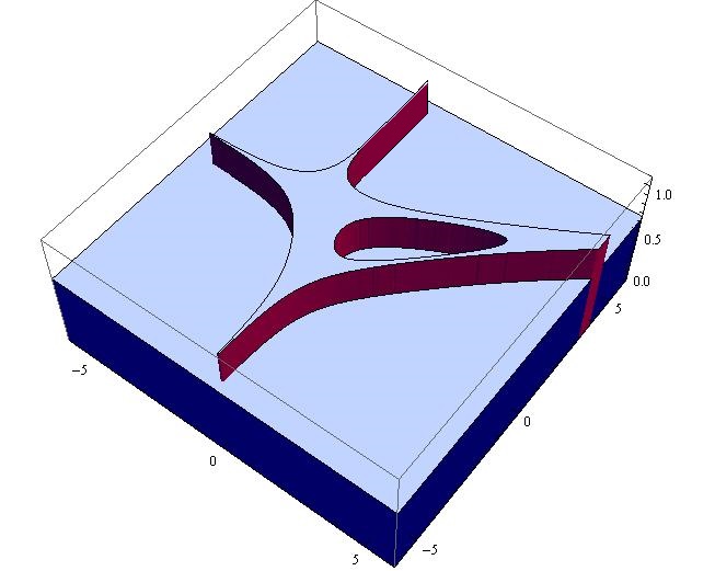
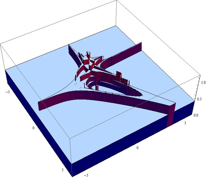
Figure 8 indicates that curves and hypersurfaces which compose higher strata may intersect in contrast to the stratum $\mathcal{Z}_{\mathrm{sing},1}$.

In general, one has

Maximum number of intersections in stratum $\mathcal{Z}_{\mathrm{sing},k}$ is bounded by one-half of the number of different pairs $\mathcal{I}_{1}$ and $\mathcal{I}_{2}$ with ${\displaystyle\#\mathcal{I}_{1}=\#\mathcal{I}_{2}=k\leq\left\lfloor\frac{N}{2}\right\rfloor}$ such that $\mathcal{I}_{1}\cap\mathcal{I}_{2}\neq\emptyset$. There are ${\displaystyle\binom{N}{k}}$ different partitions $(\mathcal{I},[N]\backslash\mathcal{I})$ of $[N]$ with cardinality $\#\mathcal{I}=k$ and for each such $\mathcal{I}$ there are ${\displaystyle\binom{N}{k}-1-\binom{N-k}{k}}$ partitions $(\mathcal{J},[N]\backslash\mathcal{J})$, $\mathcal{J}\neq\mathcal{I}$ and $\mathcal{I}\cap\mathcal{J}\neq\emptyset$. Then the number of intersections in the stratum $\mathcal{Z}_{\mathrm{sing},k}$ is bounded from above by ${\displaystyle\frac{1}{2}\cdot\binom{N}{k}\cdot\left[\binom{N}{k}-1-\binom{N-k}{k}\right]}$. It is not always a strict bound since some of these intersections might be unreachable. For example, at $k=2$ one has $\#(\mathcal{I}_{1}\cap\mathcal{I}_{2})=1$ and, hence, $\mathcal{I}_{1}=\{\alpha,\gamma_{1}\}$ and $\mathcal{I}_{2}=\{\alpha,\gamma_{2}\}$ for some $\alpha\neq\gamma_{1}\neq\gamma_{2}\neq\alpha$. Then, if $\boldsymbol{\bar{x}}$ is in the intersection $\mathcal{Z}_{\mathrm{sing},2}(\mathcal{I}_{1})\cap\mathcal{Z}_{\mathrm{sing},2}(\mathcal{I}_{2})$ one has ${\displaystyle e^{f_{\gamma_{1}}(\bar{\boldsymbol{x}})}-e^{f_{\gamma_{2}}(\bar{\boldsymbol{x}})}=-e^{f_{\alpha}(\boldsymbol{\bar{x}})}+\sum_{\beta\neq\alpha,\gamma_{1},\gamma_{2}}e^{f_{\beta}(\boldsymbol{\bar{x}})}=e^{f_{\gamma_{2}}(\boldsymbol{\bar{x}})}-e^{f_{\gamma_{1}}(\boldsymbol{\bar{x}})}}$, thus $f_{\gamma_{1}}(\boldsymbol{\bar{x}})=f_{\gamma_{2}}(\boldsymbol{\bar{x}})$ and ${\displaystyle e^{f_{\alpha}(\boldsymbol{\bar{x}})}=\sum_{\beta\neq\alpha,\gamma_{1},\gamma_{2}}e^{f_{\beta}(\boldsymbol{\bar{x}})}}$. This last equation not always has real solutions for general choice of functions.

In general, intersections of hypersurfaces (3.5) for the stratum $\mathcal{Z}_{\mathrm{sing},k}$ are not necessarily transversal. Moreover, the assumption of real-valued functions opens up the way to reductions. For example, take two functions $g(\boldsymbol{x})$ and $h(\boldsymbol{x})$ and consider $f_{1}(\boldsymbol{x})\equiv 4\cdot g(\boldsymbol{x})$, $f_{2}(\boldsymbol{x})\equiv 4\cdot h(\boldsymbol{x})$, $f_{3}(\boldsymbol{x})\equiv\ln 6+2\cdot g(\boldsymbol{x})+2\cdot h(\boldsymbol{x})$, $f_{4}(\boldsymbol{x})=\ln 4+3\cdot g(\boldsymbol{x})+h(\boldsymbol{x})$, $f_{5}(\boldsymbol{x})=\ln 4+g(\boldsymbol{x})+3\cdot h(\boldsymbol{x})$. Then $\mathcal{Z}_{2}(\{4,5\};\boldsymbol{x})={\displaystyle\left(e^{2g(\boldsymbol{x})}+e^{2h(\boldsymbol{x})}-e^{\ln 2+g(\boldsymbol{x})+h(\boldsymbol{x})}\right)^{2}}\geq 0$ and it vanishes if and only if $e^{2g(\boldsymbol{x})}+e^{2h(\boldsymbol{x})}=e^{\ln 2+g(\boldsymbol{x})+h(\boldsymbol{x})}$. From Arithmetic-Geometric inequality, this is equivalent to the algebraic constraint $g(\boldsymbol{x})=h(\boldsymbol{x})$. Occurrence of such non-transversal crossings or reductions is a particular case and influences the investigation on equilibrium and non-equilibrium regions. We assume hereafter that pairwise intersections between hypersurfaces defined by $\mathcal{Z}_{k}(\mathcal{I})=0$ or $f_{\alpha}(\boldsymbol{x})-f_{\beta}(\boldsymbol{x})=0$, $1\leq\alpha<\beta\leq N$ are transversal.

All hypersurfaces (3.4) which compose the stratum $\mathcal{Z}_{\mathrm{sing},k}$ divide $\mathbb{R}^{n}$ in a number of regions which we will call domains. Then, let us denote the subdomain in $\mathbb{R}^{n}$ where all functions $\mathcal{Z}_{k}(\mathcal{I})>0$, $\mathcal{I}\in\mathcal{P}_{k}[N]$, as $\mathcal{D}_{k+}$. For example, blue regions in figures 1,2 and 3 represent $\mathcal{D}_{1+}$ and the red region in 8(a) represents $\mathcal{D}_{2+}$. The domain $\mathbb{R}^{n}\backslash\mathcal{D}_{k+}$ is divided by hypersurfaces $\left\{\mathcal{Z}_{k}(\mathcal{I})=0\right\}$ into subdomains where some of functions $\mathcal{Z}_{k}(\mathcal{I})$ are positive and others are negative. Let us denote $\mathcal{D}_{k-}$ as the domain where the number of negative functions $\mathcal{Z}_{k}(\mathcal{J})$ with $\mathcal{J}\in\mathcal{P}_{k}[N]$ is maximal. The hypersurfaces of the $k$-stratum are confined in certain domain which we will refer as zeros confinement domain $ZCD_{k}:=\mathbb{R}^{n}\backslash(\mathcal{D}_{k+}\cup\mathcal{D}_{k-})$. The domain $ZCD_{k}$ is a sort of intermittent shell which separate the domains $\mathcal{D}_{k+}$ and $\mathcal{D}_{k-}$ and the boundary of $\mathcal{D}_{k+}\cup ZCD_{k}$ will be referred as the extremal points of hypersurfaces composing $\mathcal{Z}_{\mathrm{sing},k}$. For the first stratum $V_{1}$ defined in (2.2) the domain $ZCD_{1}$ generically has dimension $n-1$ and consists of hypersurfaces $\left\{\boldsymbol{x}:\mathcal{Z}_{1}(\{\alpha\};\boldsymbol{x})=0\right\}$, $\alpha=1,\dots,N$ themselves. For higher $V_{k}$, $k\geq 2$, the domain $ZCD_{k}$ has generically dimension $n$ and its boundary is tipically formed by pieces of different hypersurfaces belonging to $\mathcal{Z}_{\mathrm{sing},k}$.

Since at $\mathcal{D}_{k+}$ the partition function $\mathcal{Z}_{k}\equiv\mathcal{Z}|_{V_{k}}>0$ it is natural to refer to the domain $\mathcal{D}_{k+}$ as stability (equilibrium) domain. It is surrounded by the domain $ZCD_{k}$ with rather complicated singularity structure. The domain $\mathcal{D}_{k-}$ is an ambient instability domain.

These domains for different strata exhibit a simple inclusion chain.

References

• [1] L. D. Landau and E. M. Lifschitz, Statistical Physics, Course of Theoretical Physics, Part 1, Vol. 5 (Butterworth-Heinemann, 1980).
• [2] K. Huang, Statistical mechanics (New York: John Wiley & Sons, 1963).
• [3] C. N. Yang and T. D. Lee, ”Statistical theory of equations of state and phase transitions. I. Theory of condensation”, Phys. Rev. 87(3), 404-409 (1952).
• [4] T. D. Lee and C. N. Yang, ”Statistical theory of equations of state and phase transitions. II. Lattice gas and Ising model”, Phys. Rev., 87(3),410-419 (1952).
• [5] M. E. Fisher, In Lectures in Theoretical Physics, Vol. 7C, Chap. 1 (W. E. Brittin (Ed.), Boulder: University of Colorado Press, 1965)
• [6] P. J. Kortman and R. B. Griffiths, ”Density of Zeros on the Lee-Yang Circle for Two Ising Ferromagnets”, Phys. Rev. Lett. 27(21), 1439-1442 (1971).
• [7] M. Suzuki and M. E. Fisher, ”Zeros of the partition function for the Heisenberg, ferroelectric, and general Ising models”, J. Math. Phys. 12(2), 235-246, (1971)
• [8] D. Ruelle, ”Some remarks on the location of zeroes of the partition function for lattice systems”, Comm. Math. Phys. 31, 265-277 (1973).
• [9] B. Derrida, ”Random-energy model: An exactly solvable model of disordered systems”, Phys. Rev. B. 24(5), 2613-2626 (1981).
• [10] E. H. Lieb and A. D. Sokal, ”A general Lee-Yang theorem for one-component and multicomponent ferromagnets”, Commun. Math. Phys. 80(2), 153-179 (1981).
• [11] R. B. Pearson, ”Partition function of the Ising model on the periodic 4×4×44\times 4\times 4 lattice”, Phys. Rev. B 26(11), 6285-6290 (1982).
• [12] B. Derrida, L. De Seze and C. Itzykson, ”Fractal structure of zeros in hierarchical models”, J. Stat. Phys. 33(3), 559-569 (1983).
• [13] C. Borgs and R. Kotecký, ”A rigorous theory of finite-size scaling at first-order phase transitions” J. Stat. Phys. 61(1-2), 79-119 (1990).
• [14] M. Biskup, C. Borgs, J. T. Chayes, L. J. Kleinwaks, R. Kotecký, ”Partition function zeros at first-order phase transitions: A general analysis” Commun. Math. Phys. 251, 79-131 (2004).
• [15] B.-B. Wei and R.-B. Liu, ”Lee-Yang zeros and critical times in decoherence of a probe spin coupled to a bath” Phys. Rev. Lett. 109(18), (2012).
• [16] T. Obuchi and K. Takahashi, ”Dynamical singularities of glassy systems in a quantum quench”, Phys. Rev. E 86(5), (2012).
• [17] B.-B. Wei, S.-W. Chen, H.-C. Po, R.-B. Liu, ”Phase transitions in the complex plane of physical parameters”, Sci. Rep. 4, (Nature Publishing Group, 2014).
• [18] X. Peng, H. Zhou, B.-B. Wei, J. Cui, J. Du, R.-B. Liu, ”Experimental observation of Lee-Yang zeros”, Phys. Rev. Lett. 114(1), (2015).
• [19] J. S. Langer, ”Statistical theory of the decay of metastable states”, Ann. Phys. 54(2), 258-275 (1969).
• [20] C. M. Newman and L. S. Schulman, ”Complex free energies and metastable lifetimes”, J. Stat. Phys. 23(2), 131-148 (1980).
• [21] G. Parisi, ”A sequence of approximated solutions to the SK model for spin glasses”, J. Phys. A: Math. Gen. 13(4), L115-121 (1980).
• [22] M. Mezard, G. Parisi and M. A. Virasoro, Spin glass theory and beyond, (Singapore: World Scientific, 1987).
• [23] Y. Ozeki Y and H. Nishimori, ”Distribution of Yang-Lee Zeros of the ±J\pm J Ising Model”, J. Phys. Soc. Jpn. 57(3), 1087-1093 (1988).
• [24] B. Derrida, ”The zeroes of the partition function of the random energy model” Physica A 177(1-3), 31-37 (1991).
• [25] G. Bhanot and J. Lacki, ”Partition function zeros and the three-dimensional Ising spin glass”, J. Stat. Phys. 71(1-2), 259-267 (1993).
• [26] Y. Matsuda, H. Nishimori and K. Hukushima, ”The distribution of Lee-Yang zeros and Griffiths singularities in the ±J\pm J model of spin glasses”, J. Phys. A: Math. Theor. 41(32), 324012 (2008).
• [27] T. Obuchi and K. Takahashi, ”Partition-function zeros of spherical spin glasses and their relevance to chaos”, J. Phys. A: Math. Theor. 45(12), 125003, (2012).
• [28] R. P. Feynman, ”Negative probability”, in Quantum implications: essays in honour of David Bohm, 235-248 (1987).
• [29] W. D. Blizard, ”Negative membership”, Notre Dame J. Formal Logic 31(3), 346-368 (1990).
• [30] M. Burgin, ”Interpretations of negative probabilities”, arXiv preprint, arXiv:1008.1287.
• [31] K. Purbhoo, ”A Nullstellensatz for amoebas”, Duke. Math. J. 141(3), 407-445 (2008)
• [32] D. Y. Pochekutov and A. K. Tsikh, ”On the Asymptotics of Laurent Coefficients and its Application in Statistical Mechanics”, J. Siberian Fed. Univ.: Math. Phys. 2(4), 483-493 (2009).
• [33] M. Kapranov, ”Thermodynamics and the moment map”, arXiv preprint, arXiv:1108.3472 (2011).
• [34] M. Passare, D. Pochekutov, A. Tsikh, ”Amoebas of complex hypersurfaces in statistical thermodynamics” Math. Phys. Anal. Geom. 16(1), 89-108 (2012).
• [35] M. Adler and P. Van Moerbeke, ”Completely integrable systems, Euclidean Lie algebras, and curves”, Adv. Math. 38(3), 267-317 (1980).
• [36] L. Casian and Y. Kodama, ”Toda lattice, cohomology of compact Lie groups and finite Chevalley groups”, Invent. Math. 165(1), 163-208 (2006).
• [37] M. Angelelli and B. Konopelchenko, ”Geometry of the basic statistical physics mapping”, J. Phys. A: Math. Theor. 49(38), 385202 (2016).
• [38] I. M. Gelfand, M. M. Kapranov and A. V. Zelevinsky, Discriminants, Resultants, and Multidimensional Determinants, Modern Birkhäuser Classics (Boston, MA: Birkhäuser, 2008).
• [39] G. Mikhalkin, ”Real algebraic curves, the moment map and amoebas”, Ann. Math. 151(1), 309-326 (2000).
• [40] M. Forsberg, M. Passare and A. Tsikh, ”Laurent determinants and arrangements of hyperplane amoebas”, Adv. Math. 151(1), 45-70 (2000).
• [41] T. Theobald, ”Computing amoebas”, Exp. Math. 11(4), 513-526 (2002).
• [42] G. Mikhalkin, ”Amoebas of algebraic varieties and tropical geometry”, in Different faces of geometry, Int. Math. Ser. Vol. 3, 257-300 (Eds. S. Donaldson, Y. Eliashberg and M. Gromov, Springer SBM, 2004).
• [43] N. A. Bushueva and A. K. Tsikh AK, ”On amoebas of algebraic sets of higher codimension”, Proc. Steklov Inst. Math. 279(1), 52-63 (2012).
• [44] M. Nisse and M. Passare, ”Amoebas and coamoebas of linear spaces”, arXiv preprint, arXiv:1205.2808 (2012).
• [45] G. Mikhalkin, ”Amoebas of half-dimensional varieties”, arXiv preprint, arXiv:1412.4658v2 (2015).
• [46] G. Mikhalkin, ”Geometry of amoebas”, Lecture notes, Inst. Henri Poincaré (2013).
• [47] R. Kenyon, A. Okounkov and S. Sheffield, ”Dimers and amoebae”, Ann. Math. 163(3), 1019-1056 (2006).
• [48] P. Erdős, C. Ko and R. Rado, ”Intersection theorems for systems of finite sets” Q. J. Math. 12(1), 313-320 (1961)
• [49] D. Maclagan and B. Sturmfels, ”Introduction to Tropical Geometry”, Graduate Studies in Mathematics Vol. 161 (Providence, RI: Am. Math. Soc., 2015).
• [50] Y. Kodama and L. Williams, ”The Deodhar decomposition of the Grassmannian and the regularity of KP solitons”, Advances in Mathematics 244, 979-1032 (2013).
• [51] M. Angelelli and B. Konopelchenko, ”Tropical Limit in Statistical Physics”, Phys. Lett. A 379(24-25), 1497-1502 (2015).