跳到论文正文
W Papers独立论文阅读器 arXiv:1607.05831 论文正文 计算阅读时间 · 0%
引用这篇论文根据当前论文元数据生成,正式投稿前建议核对。


License: arXiv.org perpetual non-exclusive license
arXiv:1607.05831v3 [q-fin.ST] 27 Jun 2017

Statistical inference for the doubly stochastic self-exciting process

Simon Clinet Affiliation: Graduate School of Mathematical Sciences, University of Tokyo: 3-8-1 Komaba, Meguro-kuTokyo 153-8914, Japan. Email: simon@ms.u-tokyo.ac.jp, website : http://www.ms.u-tokyo.ac.jp/˜simon/ Affiliation: CREST, Japan Science and Technology Agency, Japan.    Yoann Potiron Affiliation: Faculty of Business and Commerce, Keio University. 2-15-45 Mita, Minato-ku, Tokyo, 108-8345, Japan. Phone: +81-3-5418-6571. Email: potiron@fbc.keio.ac.jp, website: http://www.fbc.keio.ac.jp/˜potiron
This version: August 24, 2026
Abstract

We introduce and show the existence of a Hawkes self-exciting point process with exponentially-decreasing kernel and where parameters are time-varying. The quantity of interest is defined as the integrated parameter T−1​∫0Tθt∗​𝑑tT^{-1}\int_{0}^{T}\theta_{t}^{*}dt, where θt∗\theta_{t}^{*} is the time-varying parameter, and we consider the high-frequency asymptotics. To estimate it naïvely, we chop the data into several blocks, compute the maximum likelihood estimator (MLE) on each block, and take the average of the local estimates. The asymptotic bias explodes asymptotically, thus we provide a non-naïve estimator which is constructed as the naïve one when applying a first-order bias reduction to the local MLE. We show the associated central limit theorem. Monte Carlo simulations show the importance of the bias correction and that the method performs well in finite sample, whereas the empirical study discusses the implementation in practice and documents the stochastic behavior of the parameters.

Keywords: Hawkes process; high-frequency data; integrated parameter ; time-varying parameter

1 Introduction

In high-frequency data, market events are observed more often than ever. As an example, the correlation between the timing of those events and other financial quantities, such as asset price, volatility and microstructure noise has become of special interest. Also, financial agents can model the order book to predict key quantities, such as the volume of trades in the next hour. For all those reasons, models for inter-arrival times, also called duration models, are needed. As a pioneer work, [16] introduced the autoregressive conditional duration (ACD) model. Other references include and are not limited to [39], [41], as well as [4], [18], and more recently [36] and [35].

The cited work is partly based on the self-exciting Hawkes point process introduced in [22] and [23]. In that model, the intensity of the point process NtN_{t} is defined as λ⁡(t):=ν+∫0tϕt−s​d​Ns\lambda(t):=\nu+\int_{0}^{t}\phi_{t-s}dN_{s}, where the baseline ν>0\nu>0. Self-exciting processes are very popular to model phenomena mainly because future events can be boosted by past events. In the high-frequency finance literature, [38] documented such time-clustering property in the order flow of several stocks. Other examples of application can be found in [15], [1], [2], [42], [28], etc. Also, [3] offers a general overview of the Hawkes process applications in finance.

We restrict our attention to the case with exponential exciting function ϕt=a​e−b​t\phi_{t}=ae^{-bt}, as studied in [31]. Time-varying parameter extensions have already been considered taking the locally stationary processes approach in [37], and restricting to the baseline time-varying case in [19], [7] and [8]. Our approach is much in line with the latter couple of work in that we consider the high-frequency point of view. In [7] the authors allow the background parameter (as they call it) ν\nu to be time-varying to incorporate intraday seasonality and consider the ACD model with time-varying background parameter. They illustrate that on data the ACD performs better when allowing for time-varying background, and that as it was already well-documented in [16] the background parameter is moving a lot intraday.

This calls into question what happens to the other two parameters aa and bb when sampling at the ultra high frequency? Do they look constant intraday? In our empirical study, we document that they are moving intraday just as the background parameter does although the intraday seasonality pattern isn’t as clear. Indeed from one day to the next, the paths are very much different and although intraday seasonality can definitely be considered as one factor, it seems that it can’t solely explain such behavior. Correspondingly we introduce a self-exciting process with stochastic time-varying parameters θt∗:=(νt∗,at∗,bt∗)\theta_{t}^{*}:=(\nu_{t}^{*},a_{t}^{*},b_{t}^{*}). The new object of interest is defined as the integrated parameter

Θ:=1T​∫0Tθt∗​𝑑t,\displaystyle\Theta:=\frac{1}{T}\int_{0}^{T}\theta_{t}^{*}dt, (1.1)

where T>0T>0 is the horizon time.

To estimate the integrated parameter (1.1), we choose to do locally MLE estimations, which was studied in a parametric context in [10], and whose numerical computation can be consulted in [33]. Specifically, if we consider Bn:=n​hn−1B_{n}:=nh_{n}^{-1} regular non-overlapping blocks of observation with time length Δn:=T​hn​n−1\Delta_{n}:=Th_{n}n^{-1}, the estimator of (1.1) is defined as

Θ^n:=1Bn​∑i=1BnΘ^i,n,\displaystyle\widehat{\Theta}_{n}:=\frac{1}{B_{n}}\sum_{i=1}^{B_{n}}\widehat{\Theta}_{i,n}, (1.2)

where Θ^i,n\widehat{\Theta}_{i,n} corresponds to the MLE applied to the market events on the iith block, nn corresponds to the number of events’ order between 00 and TT (typically the expected number of events) and the block size hnh_{n} stands for the number of events in a block’s order (typically the expected number of events on a block). The idea to use a Riemann sum of local estimates in high-frequency finance problems is very common, and can be found for example in [26] or [29]. Our own recent work includes [9]. The more general literature on local parametric approaches, when not considering the high-frequency data case, includes [17], but also [21], the locally stationary processes of [13], etc.

The first contribution of this paper is to obtain conditions on the stochastic parameter θt∗\theta_{t}^{*} and the block size hnh_{n} under which we can show a local central limit theorem (LCLT) in high-frequency asymptotics, and finiteness of moments of order 2​κ>22\kappa>2. The technique used, namely Quasi Likelihood Analysis (QLA) whose most general and powerful formulation can be consulted in [40], is not problem-specific and can very much be applied to different models. For this part, blocks with hnh_{n} which goes to infinity very slowly will be preferred, as the block length Δn\Delta_{n} will be smaller, and thus the parameter θt∗\theta_{t}^{*} almost constant on each block. In particular, if θt∗\theta_{t}^{*} is not constant, we obtain that a necessary condition is

hn=o⁡(n).h_{n}=o(\sqrt{n}). (1.3)

The second issue that this work is addressing is the asymptotic bias generated by Θ^n\widehat{\Theta}_{n}. Even in the simple parametric case, note that the bias of the MLE on each block Θ^i,n\widehat{\Theta}_{i,n} is of order hn−1h_{n}^{-1}, and thus that the bias of Θ^n\widehat{\Theta}_{n} is also of the same order hn−1h_{n}^{-1}. The asymptotic bias, i.e. the bias of the scaled error n​(Θ^n−Θ)\sqrt{n}\big(\widehat{\Theta}_{n}-\Theta\big), is thus of order n​hn−1\sqrt{n}h_{n}^{-1}. If we want to obtain no asymptotic bias, we thus need to assume that

n=o⁡(hn).\sqrt{n}=o(h_{n}). (1.4)

Thus, for that part, the block size hnh_{n} should be as large as possible.

In view of the necessary conditions (1.3) and (1.4), there is no hope to obtain any hnh_{n} for which the asymptotic bias of Θ^n\widehat{\Theta}_{n} will vanish. For that reason, we derive the one-order bias-corrected parametric MLE. Correspondingly, we define Θ^i,n(B​C)\widehat{\Theta}_{i,n}^{(BC)} as the bias-corrected MLE when fitted to the observations on the iith block. Moreover, the bias-corrected estimator of (1.1) is defined as

Θ^n(B​C):=1Bn​∑i=1BnΘ^i,n(B​C).\displaystyle\widehat{\Theta}_{n}^{(BC)}:=\frac{1}{B_{n}}\sum_{i=1}^{B_{n}}\widehat{\Theta}_{i,n}^{(BC)}. (1.5)

We provide conditions under which Θ^n(B​C)\widehat{\Theta}_{n}^{(BC)} has no asymptotic bias. Finally, the global central limit theorem (GCLT) is obtained as an immediate consequence of the finiteness of moments of order 2​κ2\kappa, the LCLT and the fact that the asymptotic bias of Θ^n(B​C)\widehat{\Theta}_{n}^{(BC)} is null.

The following section provides the setup, Section 33 develops the statistical underpinning for the time-varying self-exciting process case and Section 44 introduces the general model. In Section 55, we discuss the main results. We give some practical guidance about the implementation of the statistical procedure in Section 66. We also carry out numerical simulations in Section 77, and give an empirical illustration on real tick-by-tick data in section 88. Finally, Section 99 concludes. Proofs can be found in the Annex.

2 The setup

In this work, the terminology "market event" should be understood as possibly corresponding to a time of trade, bid or ask order (limit or market), an order of cancellation, the time of a price change, etc. We need to introduce some notation first, that will be used throughout this work. For any stochastic process XtX_{t}, we define 𝐅X=(ℱtX)t∈[0,T]{\bf F}^{X}=({\cal F}_{t}^{X})_{t\in[0,T]}, where ℱtX=σ{Xs,0≤s≤t}{\cal F}_{t}^{X}=\sigma\{X_{s},0\leq s\leq t\} designates the canonical filtration generated by XtX_{t}. We assume that NtnN_{t}^{n} is a point process, which counts the number of events on [0,t][0,t]. It means that d​Ntn=1dN_{t}^{n}=1 if there is a market event at time tt and d​Ntn=0dN_{t}^{n}=0 if not. Moreover, we assume that there is no jump at time 00 and thus that d​N0n=0dN_{0}^{n}=0. Correspondingly, we define the intensity of market events λ∗n​(t)\lambda_{*}^{n}(t). The intensity process can be thought as the instantaneous expected number of events, i.e. λ∗n​(t)​d​t=𝔼⁡[d​Ntn|ℱt(θ∗,Nn)]\lambda_{*}^{n}(t)dt=\mathbb{E}\left[dN_{t}^{n}|{\cal F}_{t}^{(\theta^{*},N^{n})}\right], where ℱt(θ∗,Nn){\cal F}_{t}^{(\theta^{*},N^{n})} is the filtration generated by ℱtθ∗{\cal F}_{t}^{\theta^{*}} and ℱtNn{\cal F}_{t}^{N^{n}}. For definitions, the reader can consult [14] or [27] for more general results about the compensator of a point process.

There are commonly two ways to make the number of events go to infinity. The low-frequency asymptotics assume that T→∞T\rightarrow\infty. [10] took this approach in an ergodic framework. On the contrary, the high-frequency point of view (also sometimes called heavy traffic asymptotics) assumes that TT is fixed, and that the number of events explodes on [0,T][0,T]. We adopt the latter approach and further consider a sequence of intensities such that 𝔼⁡[λ∗n​(t)]\mathbb{E}[\lambda_{*}^{n}(t)] is exactly of order nn, with n→∞n\rightarrow\infty. This yields a number of observations NTnN_{T}^{n} of order nn, so that we are in the classical framework of the large-sample theory.

3 Outline of the problem: an illustrative example

We start our theoretical exposition by the introduction of a point process toy model which provides an insight on the difficulties to overcome when considering the self-exciting model case. For the sake of simplicity, we stay at a heuristic level. The continuous parameter θt∗\theta_{t}^{*} is assumed to be 1-dimensional throughout the rest of this section. The parameter θt∗\theta_{t}^{*} is also restricted to belong to a compact set K=[θ¯,θ¯]K=\big[\underline{\theta},\overline{\theta}\big], where θ¯>0\underline{\theta}>0. Moreover, θt∗\theta_{t}^{*} is assumed to be adapted to some filtration ℱt{\cal F}_{t}, and to satisfy uniformly in 0≤s<t≤T0\leq s<t\leq T that 𝔼s​[|θt∗−θs∗|p]=Oℙ​((t−s)p)\mathbb{E}_{s}\big[|\theta_{t}^{*}-\theta_{s}^{*}|^{p}\big]=O_{\mathbb{P}}((t-s)^{p}), where 𝔼s[.]\mathbb{E}_{s}[.] denotes the conditional expectation with respect to ℱs{\cal F}_{s}. Finally, we assume that the process NtnN_{t}^{n} is adapted to ℱt{\cal F}_{t} and follows the dynamic of a doubly stochastic Poisson process (or Cox process) whose underlying stochastic intensity is assumed to be defined as λ∗n​(t)=n​θt∗\lambda_{*}^{n}(t)=n\sqrt{\theta_{t}^{*}}.

The estimation procedure Θ^n\widehat{\Theta}_{n} follows [34]. We are interested in assessing the GCLT n(Θ^n−Θ)→dVT12𝒩(0,1)\sqrt{n}(\widehat{\Theta}_{n}-\Theta)\to^{d}V_{T}^{\frac{1}{2}}\mathcal{N}(0,1), where the asymptotic random variance VT=T−1​∫0Tvt​𝑑tV_{T}=T^{-1}\int_{0}^{T}v_{t}dt is independent from 𝒩⁡(0,1)\mathcal{N}(0,1). Since the parameter θt∗\theta_{t}^{*} is smooth, we obtain

Θ=1Bn​∑i=1Bnθ(i−1)​Δn∗+Oℙ​(Δn).\displaystyle\Theta=\frac{1}{B_{n}}\sum_{i=1}^{B_{n}}\theta_{(i-1)\Delta_{n}}^{*}+O_{\mathbb{P}}(\Delta_{n}). (3.1)

Consequently, the GCLT will follow if we can prove that

nBn∑i=1Bn(Θ^i,n−θ(i−1)​Δn∗)→dVT12𝒩(0,1).\displaystyle\frac{\sqrt{n}}{B_{n}}\sum_{i=1}^{B_{n}}\big(\widehat{\Theta}_{i,n}-\theta_{(i-1)\Delta_{n}}^{*}\big)\to^{d}V_{T}^{\frac{1}{2}}\mathcal{N}(0,1). (3.2)

We focus on how to obtain (3.2) in this simple toy model. To do that, we rewrite the left hand-side of (3.2) as a sum of a martingale triangular array and an array of biases. Formally, (3.2) is expressed as

nBn​∑i=1BnMi,n⏟Sn(M)+nBn​∑i=1BnBi,n⏟Sn(B)→dVT12𝒩(0,1),\displaystyle\underbrace{\frac{\sqrt{n}}{B_{n}}\sum_{i=1}^{B_{n}}{M_{i,n}}}_{S_{n}^{(M)}}+\underbrace{\frac{\sqrt{n}}{B_{n}}\sum_{i=1}^{B_{n}}{B_{i,n}}}_{S_{n}^{(B)}}\to^{d}V_{T}^{\frac{1}{2}}\mathcal{N}(0,1), (3.3)

where Mi,n=Θ^i,n−θ(i−1)​Δn∗−𝔼(i−1)​Δn​[Θ^i,n−θ(i−1)​Δn∗]M_{i,n}=\widehat{\Theta}_{i,n}-\theta_{(i-1)\Delta_{n}}^{*}-\mathbb{E}_{(i-1)\Delta_{n}}\big[\widehat{\Theta}_{i,n}-\theta_{(i-1)\Delta_{n}}^{*}\big] and Bi,n=𝔼(i−1)​Δn​[Θ^i,n−θ(i−1)​Δn∗]B_{i,n}=\mathbb{E}_{(i-1)\Delta_{n}}\big[\widehat{\Theta}_{i,n}-\theta_{(i-1)\Delta_{n}}^{*}\big]. Our strategy to show (3.3) relies thus on exploiting the martingale decomposition on the left hand side of (3.3) to show that the covariances between blocks are negligible. More precisely, we want to prove that Sn(M)→dVT12𝒩(0,1)S_{n}^{(M)}\to^{d}V_{T}^{\frac{1}{2}}\mathcal{N}(0,1) on the one hand, and that Sn(B)→ℙ0S_{n}^{(B)}\to^{\mathbb{P}}0 on the other hand. To show the former statement, classical sufficient conditions (see for instance Corollary 3.1 of pp. 58-59 in [20], or also Theorem VIII.3.33 in [27]) will hold if11 1 The reader can find more details in Section 10.5 uniformly in i∈{1,…,Bn}i\in\{1,...,B_{n}\} we can show that

𝔼(i−1)​Δn​[(hn​(Θ^i,n−θ(i−1)​Δn∗))2]=v(i−1)​Δn+oℙ​(1),\displaystyle\mathbb{E}_{(i-1)\Delta_{n}}\left[\left(\sqrt{h_{n}}\left(\widehat{\Theta}_{i,n}-\theta_{(i-1)\Delta_{n}}^{*}\right)\right)^{2}\right]=v_{(i-1)\Delta_{n}}+o_{\mathbb{P}}(1), (3.4)

and for some κ>1\kappa>1 that

𝔼(i−1)​Δn​[|hn​(Θ^i,n−θ(i−1)​Δn∗)|2​κ]=Oℙ​(1).\displaystyle\mathbb{E}_{(i-1)\Delta_{n}}\left[\left|\sqrt{h_{n}}\left(\widehat{\Theta}_{i,n}-\theta_{(i-1)\Delta_{n}}^{*}\right)\right|^{2\kappa}\right]=O_{\mathbb{P}}(1). (3.5)

If we show the LCLT, i.e. the convergence of hn(Θ^i,n−θ(i−1)​Δn∗)→dv(i−1)​Δn12𝒩(0,1)\sqrt{h_{n}}(\widehat{\Theta}_{i,n}-\theta_{(i-1)\Delta_{n}}^{*})\to^{d}v_{(i-1)\Delta_{n}}^{\frac{1}{2}}\mathcal{N}(0,1) uniformly in the block number i∈{1,⋯,Bn}i\in\{1,\cdots,B_{n}\}, we can deduce from (3.5) that (3.4) holds. This will be our strategy to show that Sn(M)→dVT12𝒩(0,1)S_{n}^{(M)}\to^{d}V_{T}^{\frac{1}{2}}\mathcal{N}(0,1). Moreover, to obtain the GCLT (3.3), we also need to show that the array of biases vanishes asymptotically. Accordingly, we will look at how to obtain those three conditions (boundedness of local moments of order 2​κ2\kappa, LCLT and no asymptotic bias) in the toy model.

To fix ideas, we provide one way, which turns out to be helpful when estimating (1.1), to obtain asymptotic properties of the MLE in the parametric case when the intensity of the point process NtnN_{t}^{n} is defined as λ∗n​(t):=n​θ∗\lambda_{*}^{n}(t):=n\sqrt{\theta^{*}}. The log-likelihood of the parametric model can be expressed up to a constant additive term as

ln​(θ)=log​(θ)​NTn−n​θ​T,\displaystyle l_{n}(\theta)=\text{log}\left(\sqrt{\theta}\right)N_{T}^{n}-n\sqrt{\theta}T, (3.6)

whose maximizer θ^n\hat{\theta}_{n} admits the explicit form

θ^n=(NTnn​T)2.\displaystyle\hat{\theta}_{n}=\left(\frac{N_{T}^{n}}{nT}\right)^{2}. (3.7)

If we introduce the martingale N~tn=Ntn−n​θ∗​t\tilde{N}_{t}^{n}=N_{t}^{n}-n\sqrt{\theta^{*}}t, we can rewrite θ^n\hat{\theta}_{n} as a function of N~Tn\tilde{N}_{T}^{n}:

θ^n=θ∗+2​θ∗n​T​N~Tn+(N~Tnn​T)2.\displaystyle\hat{\theta}_{n}=\theta^{*}+\frac{2\sqrt{\theta^{*}}}{nT}\tilde{N}_{T}^{n}+\left(\frac{\tilde{N}_{T}^{n}}{nT}\right)^{2}. (3.8)

As a consequence of classical limit theorems on martingales (see, e.g., Theorem 2.28 of p. 152 in [30] if we interpolate N~tn\tilde{N}_{t}^{n} as a continuous martingale, or the more general Theorem IX.7.3 in p. 584 of [27]), we obtain the CLT

n(θ^n−θ∗)→dT−12Γ(θ∗)−12𝒩(0,1),\sqrt{n}(\hat{\theta}_{n}-\theta^{*})\to^{d}T^{-\frac{1}{2}}\Gamma(\theta^{*})^{-\frac{1}{2}}\mathcal{N}(0,1),

where the Fisher information has the form Γ⁡(θ∗)=14​(θ∗)−32\Gamma(\theta^{*})=\frac{1}{4}(\theta^{*})^{-\frac{3}{2}}. We also have the stronger statement that for any p≥1p\geq 1:

𝔼⁡[(n​(θ^n−θ∗))p]→𝔼⁡[(T−12​Γ​(θ∗)−12​ξ)p],\displaystyle\mathbb{E}\left[\left(\sqrt{n}(\hat{\theta}_{n}-\theta^{*})\right)^{p}\right]\to\mathbb{E}\left[\left(T^{-\frac{1}{2}}\Gamma(\theta^{*})^{-\frac{1}{2}}\xi\right)^{p}\right], (3.9)

where ξ\xi follows a 𝒩⁡(0,1)\mathcal{N}(0,1). Finally, we can also compute in (3.8) the finite-sample bias of the MLE

𝔼⁡[θ^n−θ∗]=θ∗n​T.\displaystyle\mathbb{E}\big[\hat{\theta}_{n}-\theta^{*}\big]=\frac{\sqrt{\theta^{*}}}{nT}. (3.10)

We are now back to the time-varying parameter model case λ∗n​(t)=n​θt∗\lambda_{*}^{n}(t)=n\sqrt{\theta_{t}^{*}}. In that case, we adapt the definition of the martingale as N~tn=Ntn−n​∫0tθs∗​𝑑s\tilde{N}_{t}^{n}=N_{t}^{n}-n\int_{0}^{t}\sqrt{\theta_{s}^{*}}ds. Working out from the explicit form (3.7), the local MLE can be expressed as

Θ^i,n=(N~i​Δnn−N~(i−1)​Δnnhn​T)2+2hn2​T2​(N~i​Δnn−N~(i−1)​Δnn)​∫(i−1)​Δni​Δnn​θs∗​𝑑s\displaystyle\widehat{\Theta}_{i,n}=\left(\frac{\tilde{N}_{i\Delta_{n}}^{n}-\tilde{N}_{(i-1)\Delta_{n}}^{n}}{h_{n}T}\right)^{2}+\frac{2}{h_{n}^{2}T^{2}}(\tilde{N}_{i\Delta_{n}}^{n}-\tilde{N}_{(i-1)\Delta_{n}}^{n})\int_{(i-1)\Delta_{n}}^{i\Delta_{n}}{n\sqrt{\theta_{s}^{*}}ds}
+1hn2​T2​(∫(i−1)​Δni​Δnn​θs∗​𝑑s)2.\displaystyle+\frac{1}{h_{n}^{2}T^{2}}\left(\int_{(i-1)\Delta_{n}}^{i\Delta_{n}}{n\sqrt{\theta_{s}^{*}}ds}\right)^{2}. (3.11)

In view of (3.11) and under the assumption that hn=o⁡(n23)h_{n}=o(n^{\frac{2}{3}}), it is easy to obtain the LCLT with local conditional variance vs=T−1​Γ​(θs∗)−1v_{s}=T^{-1}\Gamma\big(\theta_{s}^{*}\big)^{-1} and the boundedness of moments of order 2​κ2\kappa. It remains to control the array of biases Sn(B)S_{n}^{(B)}. Calculation gives us

Bi,n=θ(i−1)​Δn∗hn​T+Oℙ​(Δn),\displaystyle B_{i,n}=\frac{\sqrt{\theta_{(i-1)\Delta_{n}}^{*}}}{h_{n}T}+O_{\mathbb{P}}(\Delta_{n}), (3.12)

where the residual term Oℙ​(Δn)O_{\mathbb{P}}(\Delta_{n}), which was not part of the parametric bias (3.10), is due to the deviation of θt∗\theta_{t}^{*}. In order to obtain no asymptotic bias, we assume that n=o⁡(hn)\sqrt{n}=o(h_{n}). Consequently, if we assume that hn=n1/δh_{n}=n^{1/\delta} with 32<δ<2\frac{3}{2}<\delta<2, we can prove the GCLT with asymptotic variance VT=T−2​∫0TΓ​(θt∗)−1​𝑑tV_{T}=T^{-2}\int_{0}^{T}{\Gamma\left(\theta_{t}^{*}\right)^{-1}dt} in this toy model . This is a simple example where no further bias correction is needed to obtain the GCLT. However, in the time-varying self-exciting model, we will require to bias correct the estimator. This could be done in this simple setting via

Θ^i,n(B​C)=Θ^i,n−Θ^i,nhn​T.\displaystyle\widehat{\Theta}_{i,n}^{(BC)}=\widehat{\Theta}_{i,n}-\frac{\sqrt{\widehat{\Theta}_{i,n}}}{h_{n}T}. (3.13)

4 The model

We introduce in this section the time-varying self-exciting process, which will also be called the doubly stochastic Hawkes process, in analogy with the doubly stochastic Poisson process introduced in [11]. We first recall the definition of the non time-varying self-exciting point process. In the parametric case, the point process NtP,nN_{t}^{P,n} can be defined via its intensity function

λ∗P,n​(t)=n​ν∗+∫0t−n​a∗​e−n​b∗​(t−s)​d​NsP,n,\displaystyle\lambda_{*}^{P,n}(t)=n\nu^{*}+\int_{0}^{t-}{na^{*}e^{-nb^{*}(t-s)}dN_{s}^{P,n}}, (4.1)

where θ∗=(ν∗,a∗,b∗)\theta^{*}=(\nu^{*},a^{*},b^{*}) is the 3-dimensional parameter. The self-excitation property can be read directly from the intensity form λ∗P,n\lambda_{*}^{P,n} in (4.1). Indeed, a market event arriving at time tt will immediately boost the intensity, with an additional factor of magnitude n​a∗na^{*}, favoring the occurrence of new events in the close future. The excitation then exponentially fades away after a time of order (n​b∗)−1\left(nb^{*}\right)^{-1}. We explain now our choice regarding the asymptotics. First, we assume that the baseline intensity is proportional to nn to boost the average rate of spontaneous events. Moreover, we assume that the excitation variables are of magnitude (n​a∗,n​b∗)(na^{*},nb^{*}) in order to preserve the proportionality between the typical excitation time after a market event, (n​b∗)−1\left(nb^{*}\right)^{-1}, and the average inter-arrival time between two spontaneous events (n​ν∗)−1(n\nu^{*})^{-1}. To wrap it up, NtnN_{t}^{n} is a self-exciting process with parameters (n​ν∗,n​a∗,n​b∗)(n\nu^{*},na^{*},nb^{*}). Note that other choices can lead to fairly different asymptotics such as the ones in [32] where authors suggested a model with baseline n​ν∗n\nu^{*} but a constant excitation kernel of the form a∗​e−b∗​ta^{*}e^{-b^{*}t}.

We consider now the time-varying case. We assume that the 3-dimensional time-varying parameter process θt∗\theta_{t}^{*} is component-wise positive and is confined into the interior of a compact space KK. This implies the existence of two non-negative vectors θ¯\underline{\theta} and θ¯\overline{\theta} such that 0<θ¯≤θ≤θ¯0<\underline{\theta}\leq\theta\leq\overline{\theta} for any θ∈K\theta\in K, where the inequalities should be read component-wise. Moreover, we assume that NtnN_{t}^{n} admits the ℱt{\cal F}_{t}-stochastic intensity λ∗n​(t)\lambda_{*}^{n}(t) defined as

λ∗n(t)=nνt∗+∫0t−nas∗e−n​bs∗​(t−s)dNsn, t∈(0,T],\displaystyle\lambda_{*}^{n}(t)=n\nu_{t}^{*}+\int_{0}^{t-}{na_{s}^{*}e^{-nb_{s}^{*}(t-s)}dN_{s}^{n}},\text{ }t\in(0,T], (4.2)

where NtnN_{t}^{n} and θt∗\theta_{t}^{*} are adapted to ℱt{\cal F}_{t}22 2 The formal definition of ℱt{\cal F}_{t} can be found in Section 5., and N0n=0N_{0}^{n}=0 a.s. The time-varying model (4.2) is a natural time-varying parametric model extension of (4.1). It is constructed in the same spirit as for the doubly stochastic Poisson process, in the sense that conditionally on the path of θt∗\theta_{t}^{*}, NtnN_{t}^{n} is distributed as a standard inhomogeneous Hawkes process. The formal definition of such a property along with the existence of the doubly stochastic Hawkes process can be found in Theorem 5.1. Finally, note that the time-varying parameter model (4.2) is more general than the parametric model (4.1). In particular, the intensity between two market events is not exponentially decreasing, but rather a sum of decreasing exponential functions, each one with its own starting point and decreasing rate.

5 Main Results

5.1 Preliminary results

We present in this section general results for the doubly stochastic Hawkes process. We start by stating basic conditions on a given parameter process θt\theta_{t} that ensure the existence of the related doubly stochastic Hawkes process.

[E​​

]

(i)
r:=supt∈[0,T]atbt<1 ℙ−a.s.\displaystyle r:=\sup_{t\in[0,T]}\frac{a_{t}}{b_{t}}<1\text{ }\mathbb{P}-a.s. (5.1)
(ii)
∫0Tνsds<+∞ ℙ−a.s.\displaystyle\int_{0}^{T}\nu_{s}ds<+\infty\text{ }\mathbb{P}-a.s. (5.2)

First, note that (5.1) is not harmful. Indeed, the corresponding condition for the existence of the parametric model is ab<1\frac{a}{b}<1. Moreover, when estimating parameters by local MLE, we need θt\theta_{t} to be contained within a compact set. Thus, (5.2) will be verified automatically in that context. The next theorem shows the existence of the doubly stochastic Hawkes process associated with the process θt\theta_{t}. We recall that ℱtθ{\cal F}_{t}^{\theta} designates the canonical filtration associated with θt\theta_{t}. Moreover, the following bigger filtration ℱt{\cal F}_{t} is introduced for the construction of the doubly stochastic Hawkes process. We define the filtration as ℱt=ℱt(θ,N¯)=ℱtθ∨ℱtN¯{\cal F}_{t}={\cal F}_{t}^{(\theta,\overline{N})}={\cal F}_{t}^{\theta}\vee{\cal F}_{t}^{\overline{N}}, where N¯t=N¯​([0,t]×ℝ)\overline{N}_{t}=\overline{N}([0,t]\times\mathbb{R}) is a Poisson process of intensity 11 on ℝ2\mathbb{R}^{2} which is independent from θt\theta_{t}.

Theorem 5.1.

(Existence) Under [E], there exists a point process NtN_{t} adapted to ℱt{\cal F}_{t} such that its ℱt{\cal F}_{t}-intensity has the representation

λ⁡(t)=νt+∫0t−as​e−bs​(t−s)​d​Ns.\displaystyle\lambda(t)=\nu_{t}+\int_{0}^{t-}{a_{s}e^{-b_{s}(t-s)}dN_{s}}. (5.3)

Moreover, conditionally on the path of θt\theta_{t}, NtN_{t} is distributed as a standard Hawkes process with inhomogeneous deterministic parameter θt\theta_{t}, that is

𝔼[f(N)|ℱTθ]=𝔼[f(Nθ~)]|θ~=θ,\displaystyle\mathbb{E}\left[f(N)\left|{\cal F}_{T}^{\theta}\right.\right]=\mathbb{E}\left[f\left(N^{\tilde{\theta}}\right)\right]_{|\tilde{\theta}=\theta}, (5.4)

for any continuous bounded function ff, and where Ntθ~N_{t}^{\tilde{\theta}} is a doubly stochastic Hawkes process with underlying deterministic process θ~t\tilde{\theta}_{t}.

From now on we assume that θt∗\theta_{t}^{*} satisfies Condition [E]. Under this assumption, since NtnN_{t}^{n} is a time-varying self-exciting process with parameters (n​νt∗,n​at∗,n​bt∗)(n\nu_{t}^{*},na_{t}^{*},nb_{t}^{*}), NtnN_{t}^{n} is well-defined and adapted to ℱt{\cal F}_{t}.

We describe the statistical procedure, provide a formal definition of the local MLE Θ^i,n\widehat{\Theta}_{i,n} as well as its first order bias-corrected version Θ^i,n(B​C)\widehat{\Theta}_{i,n}^{(BC)}. We state their asymptotic properties, including the main result of this paper which is the GCLT for Θ^n(B​C)\widehat{\Theta}_{n}^{(BC)} in Theorem 5.4. Recall that we have chopped our observations into BnB_{n} time blocks of the form ((i−1)​Δn,i​Δn]((i-1)\Delta_{n},i\Delta_{n}]. For any i∈{1,…,Bn}i\in\{1,...,B_{n}\} and any θ∈K\theta\in K, we consider the regression family of intensities

λi,n​(t,θ)=n​ν+∫(i−1)​Δnt−n​a​e−n​b​(t−s)​d​Nsn,\displaystyle\lambda^{i,n}(t,\theta)=n\nu+\int_{(i-1)\Delta_{n}}^{t-}{nae^{-nb(t-s)}dN_{s}^{n}}, (5.5)

defined for t∈((i−1)​Δn,i​Δn]t\in((i-1)\Delta_{n},i\Delta_{n}]. We now define the Quasi Log Likelihood33 3 The model is by definition misspecified and thus li,nl_{i,n} is not the log likelihood function of the model. on the ii-th block as

li,n​(θ)=∫(i−1)​Δni​Δnlog​(λi,n​(t,θ))​d​Ntn−∫(i−1)​Δni​Δnλi,n​(t,θ)​𝑑t.\displaystyle l_{i,n}(\theta)=\int_{(i-1)\Delta_{n}}^{i\Delta_{n}}{\text{log}\left(\lambda^{i,n}(t,\theta)\right)dN_{t}^{n}}-\int_{(i-1)\Delta_{n}}^{i\Delta_{n}}{\lambda^{i,n}(t,\theta)dt}. (5.6)

We take the local MLE Θ^i,n\widehat{\Theta}_{i,n} as one maximizer of the Quasi Log Likelihood on the ii-th block defined as

li,n​(Θ^i,n)=maxθ∈K⁡li,n​(θ).\displaystyle l_{i,n}\left(\widehat{\Theta}_{i,n}\right)=\max_{\theta\in K}l_{i,n}(\theta). (5.7)

Looking at the form of (5.5), (5.6) and (5.7), we can see that λi,n\lambda^{i,n}, li,nl_{i,n} and Θ^i,n\widehat{\Theta}_{i,n} are functions of the ii-th block’s events44 4 Note that this doesn’t mean that Θ^i,n\widehat{\Theta}_{i,n} are uncorrelated.. In particular, we don’t take account for the possible preexcitation induced by past events in the expression of the candidate intensity (5.5), as the lower bound of the integral is fixed to (i−1)​Δn(i-1)\Delta_{n}. Asymptotically, such approximation is valid because the exponential form of the excitation kernel along with the order of the excitation parameters (n​at∗,n​bt∗)(na_{t}^{*},nb_{t}^{*}) induce a weak-enough influence of the past events on the actual stochastic intensity λ∗n​(t)\lambda_{*}^{n}(t).

In what follows we specify the form of hnh_{n} and assume the existence of an exponent δ>1\delta>1 such that

hn=n1/δ.\displaystyle h_{n}=n^{1/\delta}. (5.8)

We will also have to specify the smoothness of the process θ∗\theta^{*} using the following quantities. First, define the regularity modulus of order p∈ℕ−{0}p\in\mathbb{N}-\{0\}, at time t∈[0,T]t\in[0,T] and value θ∈K\theta\in K as

wp(t,θ,r)=𝔼[suph∈[0,r∧(T−t)]|θt+h∗−θt∗|p|ℱt,θt∗=θ], r>0.\displaystyle w_{p}(t,\theta,r)=\mathbb{E}\left[\left.\sup_{h\in[0,r\wedge(T-t)]}|\theta_{t+h}^{*}-\theta_{t}^{*}|^{p}\right|{\cal F}_{t},\theta_{t}^{*}=\theta\right],\text{ }r>0. (5.9)

We then define the global regularity modulus as

wp(r)=sup(t,θ)∈[0,T]×Kwp(t,θ,r), r>0.\displaystyle w_{p}(r)=\sup_{(t,\theta)\in[0,T]\times K}w_{p}(t,\theta,r),\text{ }r>0. (5.10)

We introduce the following conditions needed to obtain the LCLT and the boundedness of moments.

[C​​

]

(i)

There exists an exponent γ∈(0,1]\gamma\in(0,1], such that for r→0r\to 0, we have

wp​(r)=Oℙ​(rγ​p).\displaystyle w_{p}(r)=O_{\mathbb{P}}\left(r^{\gamma p}\right). (5.11)
(ii)

δ\delta and γ\gamma satisfy the relation

δ>1+1γ.\displaystyle\delta>1+\frac{1}{\gamma}. (5.12)
(iii)

The excitation parameters at∗a_{t}^{*} and bt∗b_{t}^{*} satisfy

c:=sup(t,n)∈[0,T]×ℕ∫0tnas∗e−n​bs∗​(t−s)ds<1 ℙ−a.s.\displaystyle c:=\sup_{(t,n)\in[0,T]\times\mathbb{N}}\int_{0}^{t}{na_{s}^{*}e^{-nb_{s}^{*}(t-s)}ds}<1\text{ }\mathbb{P}-a.s. (5.13)

Note that the conditional expectation 𝔼[.|ℱs,θs∗=θ]\mathbb{E}\left[.|{\cal F}_{s},\theta_{s}^{*}=\theta\right] refers to the operator 𝔼[.|ℱs]\mathbb{E}[.|{\cal F}_{s}] conditioned on θs∗=θ\theta_{s}^{*}=\theta. By definition, for a ℱ{\cal F}-measurable random variable XX, if we write GX(θ)=𝔼[X|ℱs,θs∗=θ]G_{X}(\theta)=\mathbb{E}\left[X|{\cal F}_{s},\theta_{s}^{*}=\theta\right], the relationship between both expecations can be expressed as 𝔼⁡[X|ℱs]=GX​(θs∗)\mathbb{E}[X|{\cal F}_{s}]=G_{X}(\theta_{s}^{*}). The justification of the existence of 𝔼[.|ℱs,θs∗=θ]\mathbb{E}\left[.|{\cal F}_{s},\theta_{s}^{*}=\theta\right] can be found in Section 10.3. Condition [C]-(i) quantifies the regularity of the process θt∗\theta_{t}^{*} through the regularity exponent γ\gamma. A natural example of a process satisfying [C]-(i) is the drift function, i.e. of the form

θt∗=θ0∗+∫0tus∗​𝑑s,\displaystyle\theta_{t}^{*}=\theta_{0}^{*}+\int_{0}^{t}{u_{s}^{*}ds}, (5.14)

where u∗u^{*} is a stochastic process that takes its values in a compact subset of ℝ3\mathbb{R}^{3}. Another example is a smoothed version of the Brownian motion that can be obtained as follows. Take some τ>0\tau>0, a positive vector θ(M)∈ℝ3\theta^{(M)}\in\mathbb{R}^{3}, a positive diagonal matrix σ=diag​(σν,σa,σb)\sigma=\text{diag}(\sigma^{\nu},\sigma^{a},\sigma^{b}) and consider the process

θt∗=θ(M)+στ​∫t−τtWs​𝑑s,\displaystyle\theta_{t}^{*}=\theta^{(M)}+\frac{\sigma}{\tau}\int_{t-\tau}^{t}{W_{s}ds}, (5.15)

where (Wt)t∈[−τ,T](W_{t})_{t\in\left[-\tau,T\right]} is a 3-dimensional standard Brownian motion. One can confine θt∗\theta_{t}^{*} in a compact space by stopping the process WW when it reaches some critical value. This second example is useful to model the stochastic component of the parameter as a nuisance process, and we use (5.15) in our simulation study. Note that the smaller τ\tau, the less auto-correlated θt∗\theta_{t}^{*} will be, and that we would be back to a Brownian motion in the limit τ→0\tau\to 0. For both examples (5.14) and (5.15) we have γ=1\gamma=1, but note that the correlation structure of θt∗\theta_{t}^{*} may be very complex though (to do so, we can take any process ut∗u_{t}^{*} which has a complex correlation structure).

Condition [C]-(ii) controls the lower bound of hnh_{n} and is necessary to derive the LCLT and the local boundedness of moments. In particular, as γ≤1\gamma\leq 1, [C]-(ii) implies that hn=o⁡(n)h_{n}=o(\sqrt{n}). This was stated in (1.3). Finally [C]-(iii) is an additional condition that ensures the existence of moments of NnN^{n}. We can see that [C]-(iii) is automatically satisfied if a¯≤a∗≤a¯\underline{a}\leq a^{*}\leq\overline{a}, b¯≤b∗≤b¯\underline{b}\leq b^{*}\leq\overline{b} and a¯<b¯\overline{a}<\underline{b}.

We specify now the value of the exponent

κ=γ⁡(δ−1)>1,\displaystyle\kappa=\gamma(\delta-1)>1, (5.16)

where the inequality is a direct consequence of [C]-(ii). For θ∈K\theta\in K, the positive symmetric matrix Γ⁡(θ)\Gamma(\theta) is defined as the asymptotic Fisher information of a parametric Hawkes process generated by θ\theta and can be found in (10.9). The next theorem encompasses the LCLT and the local convergence of moments of order smaller than 2​κ2\kappa of the rescaled local MLE hn​(Θ^i,n−θ(i−1)​Δn∗)\sqrt{h_{n}}\left(\widehat{\Theta}_{i,n}-\theta_{(i-1)\Delta_{n}}^{*}\right).

Theorem 5.2.

(LCLT and boundedness of moments) Let L∈[0,2​κ)L\in[0,2\kappa). Under [C], we have uniformly in i∈{1,⋯,Bn}i\in\{1,\cdots,B_{n}\} that

𝔼(i−1)​Δn​[f⁡(hn​(Θ^i,n−θ(i−1)​Δn∗))]=𝔼(i−1)​Δn​[f⁡(T−12​Γ​(θ(i−1)​Δn∗)−12​ξ)]+oℙ​(1)\displaystyle\mathbb{E}_{(i-1)\Delta_{n}}\left[f\left(\sqrt{h_{n}}\left(\widehat{\Theta}_{i,n}-\theta_{(i-1)\Delta_{n}}^{*}\right)\right)\right]=\mathbb{E}_{(i-1)\Delta_{n}}\left[f\left(T^{-\frac{1}{2}}\Gamma\left(\theta_{(i-1)\Delta_{n}}^{*}\right)^{-\frac{1}{2}}\xi\right)\right]+o_{\mathbb{P}}(1) (5.17)

for any continuous function ff with |f⁡(x)|=O⁡(|x|L)|f(x)|=O(|x|^{L}) when |x|→∞|x|\to\infty , and such that ξ\xi follows a standard normal distribution and is independent of ℱ{\cal F}.

We now introduce the first-order bias-corrected local MLE for any i∈{1,…,Bn}i\in\{1,...,B_{n}\} as

Θ^i,n(B​C)=Θ^i,n−b⁡(Θ^i,n)hn​T,\displaystyle\widehat{\Theta}_{i,n}^{(BC)}=\widehat{\Theta}_{i,n}-\frac{b\left(\widehat{\Theta}_{i,n}\right)}{h_{n}T}, (5.18)

where bb is defined in (10.14), Section 10.1, and should be compared to its very similar form for the classical i.i.d case, see e.g. [12]. We finally recall the definition of the global bias-corrected estimator that was introduced in (1.5), i.e.

Θ^n(B​C)=1Bn​∑i=1BnΘ^i,n(B​C).\displaystyle\widehat{\Theta}_{n}^{(BC)}=\frac{1}{B_{n}}\sum_{i=1}^{B_{n}}\widehat{\Theta}_{i,n}^{(BC)}. (5.19)

In the next theorem, the expression x∧yx\wedge y stands for min⁡{x,y}\min\{x,y\}.

Theorem 5.3.

(bias correction) Let ϵ∈(0,1)\epsilon\in(0,1). The bias of the estimator Θ^i,n\widehat{\Theta}_{i,n} admits the expansion

𝔼(i−1)​Δn​[Θ^i,n−θ(i−1)​Δn∗]=b⁡(θ(i−1)​Δn∗)hn​T+Oℙ​(hn−ϵ⁡(κ∧32)),\displaystyle\mathbb{E}_{(i-1)\Delta_{n}}\left[\widehat{\Theta}_{i,n}-\theta_{(i-1)\Delta_{n}}^{*}\right]=\frac{b\left(\theta_{(i-1)\Delta_{n}}^{*}\right)}{h_{n}T}+O_{\mathbb{P}}\left(h_{n}^{-\epsilon\left(\kappa\wedge\frac{3}{2}\right)}\right), (5.20)

uniformly in i∈{1,…,Bn}i\in\{1,...,B_{n}\}. Moreover, the estimator Θ^i,n(B​C)\widehat{\Theta}_{i,n}^{(BC)} has the uniform bias expansion

𝔼(i−1)​Δn​[Θ^i,n(B​C)−θ(i−1)​Δn∗]=Oℙ​(hn−ϵ⁡(κ∧32)).\displaystyle\mathbb{E}_{(i-1)\Delta_{n}}\left[\widehat{\Theta}_{i,n}^{(BC)}-\theta_{(i-1)\Delta_{n}}^{*}\right]=O_{\mathbb{P}}\left(h_{n}^{-\epsilon\left(\kappa\wedge\frac{3}{2}\right)}\right). (5.21)

Now our aim is to combine Theorem 5.2 and Theorem 5.3 to state the asymptotic properties of the global estimator. In the following there are two parts. The main one gives the GCLT when the parameter is assumed to be sufficiently smooth. The second part investigates what happens when the parameter is rough.

5.2 Global central limit theorem when parameters are smooth

In this section, we state an additional condition on δ\delta and γ\gamma so that Θ^n(B​C)\widehat{\Theta}_{n}^{(BC)} is asymptotically unbiased.

[BC​​

] δ\delta and γ\gamma satisfy the relation

γγ−12<δ<3.\displaystyle\frac{\gamma}{\gamma-\frac{1}{2}}<\delta<3. (5.22)

Intuitively, the left-hand side inequality in [BC] ensures that the size of each block is not too big so that the bias induced by the parameter process θt∗\theta_{t}^{*} itself is negligible. On the contrary, the right-hand side inequality is a sufficient condition to keep under control the finite-sample bias of the local MLE by avoiding too small blocks. More precisely, Condition [BC] implies in particular that the exponent γ∈(34,1]\gamma\in\left(\frac{3}{4},1\right]. Note that such condition excludes the class of Itô-processes as a parameter process. Moreover, on (34,1]\left(\frac{3}{4},1\right] we have γγ−12≥1+1γ\frac{\gamma}{\gamma-\frac{1}{2}}\geq 1+\frac{1}{\gamma} with equality for γ=1\gamma=1, and thus [BC] is a stronger condition than [C]-(ii). For instance, in the Lipschitz case γ=1\gamma=1, [BC] (and thus [C]-(ii)) are satisfied for 2<δ<32<\delta<3. This means by definition of δ\delta that hnh_{n} must be taken so that n13=o⁡(hn)n^{\frac{1}{3}}=o(h_{n}) and hn=o⁡(n12)h_{n}=o(n^{\frac{1}{2}}).

We finally state the main result of this work which investigates the limit error of the bias-corrected estimator Θ^n(B​C)\widehat{\Theta}_{n}^{(BC)}.

Theorem 5.4.

(GCLT) Assume that [C] and [BC] hold. Then, ℱTθ∗{\cal F}_{T}^{\theta^{*}}-stably in law as n→∞n\rightarrow\infty,

n​(Θ^n(B​C)−Θ)→(T−2​∫0TΓ​(θs∗)−1​𝑑s)12​𝒩​(0,1),\displaystyle\sqrt{n}\big(\widehat{\Theta}_{n}^{(BC)}-\Theta\big)\rightarrow\left(T^{-2}\int_{0}^{T}\Gamma(\theta_{s}^{*})^{-1}ds\right)^{\frac{1}{2}}\mathcal{N}(0,1), (5.23)

where 𝒩⁡(0,1)\mathcal{N}(0,1) is independent from the σ\sigma-field ℱTθ∗\mathcal{F}_{T}^{\theta^{*}}.

Remark 5.5.

(convergence rate) The convergence rate in Theorem (5.4) is the same as in the parametric case. We also conjecture that the asymptotic variance is the non-parametric efficient bound.

Remark 5.6.

(robustness to jumps in the parameter process) We assume that we add a jump component to the parameter process

θt∗=θt(C)+θt(J),\displaystyle\theta_{t}^{*}=\theta_{t}^{(C)}+\theta_{t}^{(J)}, (5.24)

where θt(J)\theta_{t}^{(J)} denotes a 33-dimensional finite activity jump process and d​θt(J,k)d\theta_{t}^{(J,k)} is either zero (no jump) or a real number indicating the size of the jump at time tt for k=1,2,3k=1,2,3. We further assume that there is no initial jump, i.e. J0=0J_{0}=0. Moreover, we assume that JtJ_{t} is a general Poisson process independent from the other quantities. Under similar assumptions, the results of this work can be adapted.

Remark 5.7.

(mutually exciting process) The proofs can be adapted to a multidimensional Hawkes process. Investigating the corresponding conditions is beyond the scope of this paper.

5.3 What happens in the rough parameter case?

In this section, we are interested in the asymptotic properties of our estimators when the regularity condition γ∈(34,1]\gamma\in\left(\frac{3}{4},1\right] fails. We first give a theoretical argument to show that the bound 3/43/4 can be lowered to 1/21/2, although the some of the corresponding bias theoretical formula terms would be too involved to be of any practical interest. Nonetheless the bias can be computed with Monte Carlo methods (see Section 7.1 in our numerical study for more details). We then provide the expected convergence rate of the consistency for both the naive and the first order bias-corrected estimators.

When γ∉(34,1]\gamma\notin\left(\frac{3}{4},1\right], Theorem 5.4 fails in general. This is due to the bias expansion obtained in Theorem 5.3, (5.21), whose order in hn−κ∧32h_{n}^{-\kappa\wedge\frac{3}{2}} can be dominated by n−12n^{-\frac{1}{2}} only if γ>3/4\gamma>3/4. Nevertheless, we can expect that correcting for the bias to a higher order improves the rate of convergence in (5.21). Thus we would obtain a corresponding central limit theorem even for γ≤3/4\gamma\leq 3/4. A closer investigation to the proofs shows that if one conducts the bias correction up to order q∈ℕ−{0}q\in\mathbb{N}-\{0\}, conditions [C]-(ii) and [BC] are respectively replaced by δ>1+(q+1)/(2​γ)\delta>1+(q+1)/(2\gamma) and γ/(γ−1/2)<δ<2+q\gamma/(\gamma-1/2)<\delta<2+q, so that the GCLT becomes valid under the weaker condition γ∈(12+12​(1+q),1]\gamma\in\left(\frac{1}{2}+\frac{1}{2(1+q)},1\right]. For q→+∞q\to+\infty, the asymptotic admissible interval becomes thus (12,1]\left(\frac{1}{2},1\right], so it is theoretically possible to construct an asymptotically normal estimator for any γ>1/2\gamma>1/2.

When γ∈(0,12]\gamma\in(0,\frac{1}{2}], we can’t use the same martingale approach. In general, the bias induced by the parameter process in the expansion (5.21) cannot be corrected without some information on the distribution of θt∗\theta_{t}^{*}. We can’t show that the bias is of the right order, because this would imply a choice of δ\delta such that γ<δ⁡(γ−1/2)\gamma<\delta(\gamma-1/2) which is not possible if γ\gamma reaches the critical value γ=1/2\gamma=1/2. Investigating if other approaches yield a better estimate of the bias under additional specification on the structure of θt∗\theta_{t}^{*} is beyond the scope of this work.

We now turn to the convergence rate of our estimators when the central limit theorem fails. We can prove that both estimators Θ^n\widehat{\Theta}_{n} and Θ^n(B​C)\widehat{\Theta}_{n}^{(BC)} are consistent. Indeed, it turns out that the first order bias corrected version is nαn^{\alpha}-consistent55 5 An estimator Θ¯n\bar{\Theta}_{n} is said to be ana_{n}-consistent if an​(Θ¯n−Θ)=Oℙ​(1).a_{n}(\bar{\Theta}_{n}-\Theta)=O_{\mathbb{P}}(1). for any α∈(0,γ1+23​γ)\alpha\in\big(0,{\frac{\gamma}{1+\frac{2}{3}\gamma}}\big), whereas the naive estimator is only nαn^{\alpha}-consistent for any α∈(0,γ1+γ)\alpha\in\big(0,{\frac{\gamma}{1+\gamma}}\big). More specifically, we have the following result. The proposition can be showed following a similar reasoning as in the proof of Theorem 5.4.

Proposition 5.8.

(consistency) For any α∈(0,γ1+γ)\alpha\in\left(0,\frac{\gamma}{1+\gamma}\right), the choice δ∈(1+1γ,1α)\delta\in\left(1+\frac{1}{\gamma},\frac{1}{\alpha}\right) gives

nα(Θ^n−Θ)→ℙ0.n^{\alpha}(\widehat{\Theta}_{n}-\Theta)\to^{\mathbb{P}}0.

Moreover, if γ∈(0,3/4]\gamma\in(0,3/4], for any α∈(0,γ1+23​γ)\alpha\in\left(0,\frac{\gamma}{1+\frac{2}{3}\gamma}\right), the choice δ∈((1+1γ)∨γγ−α,32​α)\delta\in\left((1+\frac{1}{\gamma})\vee\frac{\gamma}{\gamma-\alpha},\frac{3}{2\alpha}\right) gives

nα(Θ^n(B​C)−Θ)→ℙ0.n^{\alpha}(\widehat{\Theta}_{n}^{(BC)}-\Theta)\to^{\mathbb{P}}0.

In particular we can see that Θ^n\widehat{\Theta}_{n} is already almost n\sqrt{n}-consistent when γ=1\gamma=1 without any bias correction. In a similar way, the case γ=3/4\gamma=3/4 also yields an almost n\sqrt{n}-consistent bias corrected estimator Θ^n(B​C)\widehat{\Theta}_{n}^{(BC)} as was expected. Again, knowing if the bounds for α\alpha given in Proposition 5.8 are optimal is beyond the scope of this paper.

6 Statistical implementation

In this section, we give some practical guidance to the above theory including a studentized version of the GCLT. Actually, on real data, the quantity of interest is n​Θn\Theta whereas nn is (usually) unknown. This doesn’t prevent us from obtaining a studentized version of the GCLT. A feasible procedure consists in estimating directly n​Θn\Theta in place of estimating Θ\Theta. When properly divided by nn, this yields the same estimate as the non feasible procedure, i.e. we have n​Θ^=n​Θ^n\widehat{\Theta}=\widehat{n\Theta}, where Θ^\widehat{\Theta} is the naive or the bias-corrected estimator. Indeed note that a maximizer Θ^i,n\widehat{\Theta}_{i,n} of li,n​(θ)l_{i,n}(\theta) is equal to n−1​Θ~i,nn^{-1}\tilde{\Theta}_{i,n}, where Θ~i,n\tilde{\Theta}_{i,n} is a maximizer of li,n​(n−1​θ)l_{i,n}(n^{-1}\theta), which corresponds to the ordinary quasi-likelihood (i.e. with disregard for the actual value of nn).

Now we provide an estimator (up to a scaling factor) of the asymptotic variance VT=T−2​∫0TΓ​(θs∗)−1​𝑑sV_{T}=T^{-2}\int_{0}^{T}\Gamma(\theta_{s}^{*})^{-1}ds, which also requires no information on the value of nn. For any i∈{1,⋯,Bn}i\in\{1,\cdots,B_{n}\}, we estimate the contribution of the ii-th block by the formula

C^i,n:=−[∂ξ2li,n(n−1ξ)|ξ=nΘ^i,n]−1.\displaystyle\widehat{C}_{i,n}:=-\left[\partial_{\xi}^{2}l_{i,n}\left(n^{-1}\xi\right)_{|\xi=n\widehat{\Theta}_{i,n}}\right]^{-1}. (6.1)

The term ∂ξ2li,n​(n−1​ξ)\partial_{\xi}^{2}l_{i,n}\left(n^{-1}\xi\right) doesn’t depend on nn (when hnh_{n} is chosen) and corresponds precisely to the Hessian matrix at point ξ\xi of the likelihood function of a Hawkes model when one disregards the value of nn. In particular, this implies that C^i,n\widehat{C}_{i,n} can be computed. The asymptotic variance is then estimated, up to a scaling factor, as the weighted sum

C^n=1Bn2​∑i=1BnC^i,n.\displaystyle\widehat{C}_{n}=\frac{1}{B_{n}^{2}}\sum_{i=1}^{B_{n}}\widehat{C}_{i,n}. (6.2)

The next proposition states the consistency of n−1​C^nn^{-1}\widehat{C}_{n} towards VTV_{T} along with a corresponding studentized version of Theorem 5.4, which is a corollary to the stable convergence in the GCLT.

Proposition 6.1.

We have

n−1C^n→ℙVT.n^{-1}\widehat{C}_{n}\to^{\mathbb{P}}V_{T}.

Moreover, we have the convergence in distribution

C^n−1/2(nΘ^n(B​C)−nΘ)→𝒩(0,1).\displaystyle\widehat{C}_{n}^{-1/2}\left(n\widehat{\Theta}_{n}^{(BC)}-n\Theta\right)\rightarrow\mathcal{N}(0,1). (6.3)

Note that C^n\widehat{C}_{n} is the asymptotic variance of the dispersion between the estimated value of the scaled integrated parameter n​Θ^n(B​C)n\widehat{\Theta}_{n}^{(BC)} and the target n​Θn\Theta itself. In particular feasible asymptotic confidence intervals can be constructed from the data.

As the value of nn is unknown, which value to choose for hnh_{n}? One idea is to normalize the value of θt∗\theta_{t}^{*} so that the expected number of events between 0 and TT is roughly one when parameters are equal to θt∗\theta_{t}^{*} (by analogy with other models in high frequency data where nn corresponds exactly to the size of the sample data, as when estimating volatility from log-price returns observed regularly at times i​T/niT/n). This amounts to taking n≈NTn\approx N_{T} in practice. Although not perfect this provides guidance to the choice of hnh_{n}, which is assumed to be n1/3=o⁡(hn)n^{1/3}=o(h_{n}) and hn=o⁡(n1/2)h_{n}=o(n^{1/2}) for a regular process (γ=1\gamma=1). In our numerical study, we have NT≈27,300N_{T}\approx 27,300 which amounts to taking n=27,300n=27,300. This gives us n1/3≈30n^{1/3}\approx 30 and n1/2≈165n^{1/2}\approx 165, and correspondingly we look at different hn=136.5,273,546h_{n}=136.5,273,546 which are of the same order. In our empirical study, we consider hn=n,2​n,4​n,8​n,16​nh_{n}=\sqrt{n},2\sqrt{n},4\sqrt{n},8\sqrt{n},16\sqrt{n}.

7 Numerical simulations

7.1 Goal of the study

In this section, we report the numerical results which assess the central limit theory of

Zn(B​C)=C^n−1/2(nΘ^n(B​C)−nΘ)→𝒩(0,1)\displaystyle Z_{n}^{(BC)}=\widehat{C}_{n}^{-1/2}\left(n\widehat{\Theta}_{n}^{(BC)}-n\Theta\right)\rightarrow\mathcal{N}(0,1)

in a finite sample context for several time-varying parameter models. In addition, we report the behavior of the studentized naive estimator

Zn=C^n−1/2(nΘ^n−nΘ).\displaystyle Z_{n}=\widehat{C}_{n}^{-1/2}\left(n\widehat{\Theta}_{n}-n\Theta\right).

Finally, we compare the performance of Θ^n(B​C)\widehat{\Theta}_{n}^{(BC)} and Θ^n\widehat{\Theta}_{n} with two concurrent methods which are

  1. 1.

    The MLE on [0,T][0,T] when considering that the parameters are not time-varying on [0,T][0,T].

  2. 2.

    The time-varying baseline intensity MLE from [7] (CH) that assumes that νt∗=f⁡(t,θ)\nu_{t}^{*}=f(t,\theta) with ff being a polynomial of order 33. More specifically in this setting the MLE estimates (θ,a,b)(\theta,a,b) where aa and bb are assumed to be constant over time.

The local log-likelihood functions and local variance estimators are computed implementing the formula obtained in [33]. To compute Θ^n(B​C)\widehat{\Theta}_{n}^{(BC)}, we can either implement the function defined in (5.18) or carry out Monte-Carlo simulations to compute bi,n​(θ)b_{i,n}(\theta) for any θ\theta prior to the numerical study. We choose the latter option as this allows to get also rid of bias terms which appears in the Taylor expansion in a higher order than 11. Indeed, although those terms vanish asymptotically, they can pop up in a finite sample context. To be more specific, we first compute the sample mean for a grid of parameter values θ\theta and a grid of block length Δ\Delta with 100,000 Monte Carlo paths of the parametric model, that we denote b⁡(θ,Δ)b(\theta,\Delta). Then on each block, we estimate the bias by b⁡(Θ^i,n,Δi,n)b(\widehat{\Theta}_{i,n},\Delta_{i,n}).

7.2 Model design

We consider that T=21,600T=21,600 seconds, which corresponds to the period of activity for one working day from 10am to 4pm. The market events are chosen to correspond to trades. The NtnN_{t}^{n} process is generated using a time-varying version of the algorithm described in [33] (Section 4, pp. 148-149). The integrated parameter is set to n​Θ≈(.8,11,30)n\Theta\approx(.8,11,30), which are comparable values to our empirical results. This yields on average NTn≈27,300N_{T}^{n}\approx 27,300 trades a day.

We consider three deterministic and one stochastic models for the time-varying parameter. The first two settings are toy models. Model I is a linear trend with θt∗=θ(M)+A⁡(−1+2​tT)\theta_{t}^{*}=\theta^{(M)}+A(-1+2\frac{t}{T}), where the non-random target value θ(M)=(.8,11,30)\theta^{(M)}=(.8,11,30) and the amplitude is set to A=(.5,4,10)A=(.5,4,10). This means that θt∗\theta_{t}^{*} takes values in [.3,1.3]×[7,15]×[20,40]\big[.3,1.3\big]\times\big[7,15\big]\times\big[20,40\big], which is comparable to the daily variation in our empirical results. In Model II θt∗\theta_{t}^{*} oscillates around θ(M)=(.8,11,30)\theta^{(M)}=(.8,11,30) and has the form θt∗=θ(M)+A​cos⁡(tT​2​π)\theta_{t}^{*}=\theta^{(M)}+A\cos(\frac{t}{T}2\pi), in particular implying that the range of taken values is the same as in Model I.

Model III is taken directly from the literature. We keep at∗a_{t}^{*} and bt∗b_{t}^{*} constant whereas νt∗\nu_{t}^{*} follows a usual intraday pattern, so that CH is well specified for this model. As pointed out in [16] (see discussions in Section 5-6 and Figure 2), the expected duration before the next trade tends to follow a U-shape intraday pattern. This diurnal effect motivated [7] (see Section 5, pp. 1011-1017) to model a Hawkes process where νt∗\nu_{t}^{*} is time-varying with a quadratic form. The model is written as νt∗=eβ1+{eβ2+eβ3}2​(t/T−eβ2/(eβ2+eβ3))2\nu_{t}^{*}=e^{\beta_{1}}+\{e^{\beta_{2}}+e^{\beta_{3}}\}^{2}(t/T-e^{\beta_{2}}/(e^{\beta_{2}}+e^{\beta_{3}}))^{2}. We fit the model to the empirical intraday mean and find β1≈−.84\beta_{1}\approx-.84, β2≈−.26\beta_{2}\approx-.26 and β3≈−.39\beta_{3}\approx-.39, which implies that T−1​∫0Tνt∗​𝑑t≈.61T^{-1}\int_{0}^{T}\nu_{t}^{*}dt\approx.61. The other two parameters (at∗,bt∗)=(11,30)(a_{t}^{*},b_{t}^{*})=(11,30) are assumed to be constant.

Model IV is an extension of Model III based on more realistic considerations where at∗a_{t}^{*} and bt∗b_{t}^{*} also feature intraday seasonality. In addition, we allow for additive stochastic component in the three parameters . We assume that

νt∗\displaystyle\nu_{t}^{*} =\displaystyle= eβ1ν+{eβ2ν+eβ3ν}2​(t/T−eβ2ν/(eβ2ν+eβ3ν))2+σν​W~tν,\displaystyle e^{\beta_{1}^{\nu}}+\{e^{\beta_{2}^{\nu}}+e^{\beta_{3}^{\nu}}\}^{2}(t/T-e^{\beta_{2}^{\nu}}/(e^{\beta_{2}^{\nu}}+e^{\beta_{3}^{\nu}}))^{2}+\sigma^{\nu}\tilde{W}_{t}^{\nu},
at∗\displaystyle a_{t}^{*} =\displaystyle= eβ1a+{eβ2a+eβ3a}2​(t/T−eβ2a/(eβ2a+eβ3a))2+σa​W~ta,\displaystyle e^{\beta_{1}^{a}}+\{e^{\beta_{2}^{a}}+e^{\beta_{3}^{a}}\}^{2}(t/T-e^{\beta_{2}^{a}}/(e^{\beta_{2}^{a}}+e^{\beta_{3}^{a}}))^{2}+\sigma^{a}\tilde{W}_{t}^{a},
bt∗\displaystyle b_{t}^{*} =\displaystyle= eβ1b+{eβ2b+eβ3b}2​(t/T−eβ2b/(eβ2b+eβ3b))2+σb​W~tb,\displaystyle e^{\beta_{1}^{b}}+\{e^{\beta_{2}^{b}}+e^{\beta_{3}^{b}}\}^{2}(t/T-e^{\beta_{2}^{b}}/(e^{\beta_{2}^{b}}+e^{\beta_{3}^{b}}))^{2}+\sigma^{b}\tilde{W}_{t}^{b},

where (β1ν,β2ν,β3ν)≈(−0.84,−0.26,−0.39)(\beta_{1}^{\nu},\beta_{2}^{\nu},\beta_{3}^{\nu})\approx(-0.84,-0.26,-0.39), (β1a,β2a,β3a)≈(2.35,−0.05,0.40)(\beta_{1}^{a},\beta_{2}^{a},\beta_{3}^{a})\approx(2.35,-0.05,0.40), and (β1b,β2b,β3b)(\beta_{1}^{b},\beta_{2}^{b},\beta_{3}^{b}) ≈(3.66CLOSE,\approx(3.66, OPEN−0.33,0.67)-0.33,0.67) were obtained when fitted to the respective parameter intraday mean. We also set (σν,σa,σb)=(0.8/(6​T1/2),11/(6​T1/2),30/(6​T1/2))(\sigma^{\nu},\sigma^{a},\sigma^{b})=(0.8/(6T^{1/2}),11/(6T^{1/2}),30/(6T^{1/2})) and W~t=(W~tν,W~ta,W~tb)=∫t−1tWs​𝑑s\tilde{W}_{t}=(\tilde{W}_{t}^{\nu},\tilde{W}_{t}^{a},\tilde{W}_{t}^{b})=\int_{t-1}^{t}W_{s}ds with Wt=(Wtν,Wta,Wtb)W_{t}=(W_{t}^{\nu},W_{t}^{a},W_{t}^{b}) a standard 3-dimensional Brownian motion. This means that the standard deviation of the noise factor is roughly equal to 1/61/6 the value of the parameter at time TT. Also, we cap the possible value taken by νt∗\nu_{t}^{*} so that the intensity parameter stays bigger than 0.20.2. It is clear that in all those models the parameter is smooth enough to satisfy the assumptions of the GCLT.

Finally, we look at several values for hn=136.5,273,546h_{n}=136.5,273,546, which correspond respectively to block lengths of size T​hn/n=Th_{n}/n= 108, 216 and 432 seconds. We have NT≈27,300N_{T}\approx 27,300 which means that we should take n=27,300n=27,300 as explained in Section 6. According to the theory we would expect to need that hnh_{n} is of the same order as n1/3n^{1/3} and n1/2n^{1/2}, which are approximately equal to 30 and 165, thus our choices for hnh_{n} seem coherent with the theory.

7.3 Results

Table 1 shows the Monte Carlo results for the feasible statistic of the naive estimator. For all the models, the value of the bias is striking as it is of the same magnitude as the standard deviation. This indicates that the bias do play a crucial role in finite sample too.

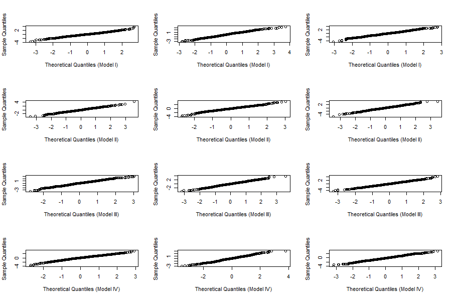
Table 2 shows the result for the bias-corrected estimator. In addition, Figure 1 provides the associated QQ-plot. In this case, the sample mean is very close to 0 indicating that our proposed reduction method is working well. The standard deviation obtained for the intensity parameter is close to 1, but it is bigger for the other parameters a∗a^{*} and b∗b^{*}. Correspondingly, the asymptotics are slightly underestimating the mass of the distribution in the tails. The reason for this is probably that it is difficult to accurately estimate the variance of the parametric model on the small blocks.

Table 3 shows the performance of the estimators with concurrent approaches. It is clear that regardless of the model at hand the bias-corrected local approach performs better than the MLE and the CH. In Model III, CH performs a MLE with no misspecification. Although CH performs much better than in the other models, it still doesn’t outperform the local approach, which indicates that the local approach can performs better even on standard parametric models. Both estimators are badly biased in case of misspecification for them. More surprisingly, although Model III follows a model included in [7] and thus CH performs a MLE with no misspecification in that specific case, the estimates are still biased (although very good for a∗a^{*} and with a smaller standard deviation).

Finally, we can see that the naive estimator is more biased when hnh_{n} is smaller, which is in line with what we expected. The bias-correction is performed better with bigger hnh_{n}, although too big of a hnh_{n} will tend to bias-correct less efficiently (due to the fact that parameters are moving too much on a bigger block). This can be seen in Table 3 as the bias-corrected estimator seems to perform slightly better with 4 minute block than 7 minute block.

Table 1: Finite sample properties of ZnZ_{n} for several models†
Param. Mean Stdv. RMSE 0.5% 2.5% 5% 95% 97.5% 99.5%
Model I
ν∗\nu^{*} 0.69 1.02 1.23 0.00 0.40 1.00 82.60 89.70 97.00
a∗a^{*} 0.77 1.10 1.34 0.40 1.00 1.50 78.00 86.50 95.90
b∗b^{*} 1.37 1.24 1.85 0.20 0.60 1.00 58.20 67.60 83.90
Model II
ν∗\nu^{*} 0.71 1.02 1.24 0.00 0.60 1.10 81.20 89.40 97.60
a∗a^{*} 0.71 1.14 1.34 0.30 1.40 2.10 79.50 86.70 94.30
b∗b^{*} 1.33 1.27 1.83 0.10 0.40 1.10 60.00 69.60 85.40
Model III
ν∗\nu^{*} 0.80 1.05 1.32 0.10 0.30 0.90 78.40 86.30 95.30
a∗a^{*} 0.78 1.14 1.38 0.00 1.20 1.70 78.10 85.70 94.10
b∗b^{*} 1.43 1.24 1.89 0.00 0.20 0.40 55.70 66.10 80.60
Model IV
ν∗\nu^{*} 0.83 0.99 1.29 0.00 0.20 0.50 79.70 87.10 96.30
a∗a^{*} 1.05 1.04 1.48 0.00 0.60 0.90 71.60 80.90 93.00
b∗b^{*} 1.62 1.10 1.96 0.00 0.10 0.20 52.20 63.20 79.70

†This table shows summary statistics and empirical quantiles benchmarked to the NN(0,1) distribution for the feasible Z-statistics related to the naive estimator with hn=273h_{n}=273 (which corresponds to a 216 second block length). The simulation design is Model I-IV with M=1,000M=1,000 Monte-Carlo simulations.

Table 2: Finite sample properties of Zn(B​C)Z_{n}^{(BC)} for several models†
Param. Mean Stdv. RMSE 0.5% 2.5% 5% 95% 97.5% 99.5%
Model I
ν∗\nu^{*} -0.01 1.02 1.02 0.40 2.80 5.70 94.70 97.20 99.30
a∗a^{*} 0.00 1.12 1.12 1.10 4.00 7.60 93.50 96.70 99.10
b∗b^{*} -0.02 1.30 1.30 2.60 6.60 10.70 90.10 93.40 98.60
Model II
ν∗\nu^{*} 0.02 1.02 1.02 0.90 2.70 5.20 95.70 98.10 99.40
a∗a^{*} -0.07 1.16 1.16 2.00 5.00 9.00 92.10 95.70 99.00
b∗b^{*} -0.08 1.32 1.33 4.20 7.60 11.50 90.50 94.30 98.20
Model III
ν∗\nu^{*} 0.00 1.05 1.05 0.10 2.90 6.20 94.30 96.90 99.50
a∗a^{*} -0.02 1.15 1.15 1.90 4.80 8.80 91.00 95.90 99.00
b∗b^{*} -0.06 1.29 1.30 4.00 7.30 11.00 90.80 94.50 98.30
Model IV
ν∗\nu^{*} 0.07 0.99 1.00 0.30 2.30 4.60 94.20 97.60 99.70
a∗a^{*} -0.04 1.05 1.05 1.20 3.50 5.40 94.90 97.30 99.30
b∗b^{*} -0.07 1.15 1.15 1.40 5.70 9.10 92.00 95.80 99.30

†This table shows summary statistics and empirical quantiles benchmarked to the NN(0,1) distribution for the feasible Z-statistics related to the bias-corrected estimator with hn=273h_{n}=273 (which corresponds to a 216 second block length). The simulation design is Model I-IV with M=1,000M=1,000 Monte-Carlo simulations.

Refer to caption
Figure 1: QQ-plots benchmarked to the NN(0,1) distribution for the feasible Z-statistics related to the bias-corrected estimator with hn=273h_{n}=273 (which corresponds to a 216 second block length). The left column corresponds to νt∗\nu_{t}^{*}, the column in the middle for at∗a_{t}^{*} and the right column for bt∗b_{t}^{*}. The simulation design is Model I-IV with M=1,000M=1,000 Monte-Carlo simulations.
Table 3: Performance of 8 estimators for several models†
ν∗\nu^{*} a∗a^{*} b∗b^{*}
Est. Mean Stdv. Mean Stdv. Mean Stdv.
Model I
naive 2m 0.009 0.007 0.286 0.196 1.239 0.630
BC 2m 0.000 0.007 -0.012 0.201 -0.124 0.658
naive 4m 0.005 0.007 0.134 0.189 0.546 0.495
BC 4m 0.000 0.007 0.002 0.192 0.005 0.503
naive 7m 0.002 0.007 0.068 0.188 0.271 0.477
BC 7m 0.000 0.007 0.004 0.189 0.010 0.481
MLE -0.011 0.006 0.489 0.198 0.485 0.494
CH 0.018 0.010 0.424 0.438 1.378 0.942
Model II
naive 2m 0.009 0.007 0.287 0.213 1.346 0.734
BC 2m 0.000 0.007 -0.018 0.218 -0.078 0.744
naive 4m 0.005 0.007 0.126 0.198 0.538 0.516
BC 4m 0.000 0.007 -0.009 0.201 -0.019 0.525
naive 7m 0.002 0.007 0.057 0.196 0.245 0.490
BC 7m 0.000 0.007 -0.009 0.197 -0.022 0.494
MLE -0.017 0.006 0.708 0.214 0.666 0.516
CH -0.063 0.012 0.294 0.443 -0.265 1.097
Model III
naive 2m 0.009 0.006 0.348 0.235 1.474 0.734
BC 2m 0.000 0.006 -0.009 0.241 -0.108 0.742
naive 4m 0.005 0.005 0.158 0.227 0.645 0.568
BC 4m 0.000 0.005 -0.003 0.241 -0.015 0.578
naive 7m 0.002 0.006 0.074 0.225 0.316 0.543
BC 7m 0.000 0.006 -0.004 0.227 -0.020 0.548
MLE -0.004 0.006 -0.081 0.220 -0.572 0.519
CH -0.009 0.005 -0.002 0.213 -0.082 0.454
Model IV
naive 2m 0.009 0.006 0.624 0.332 3.533 2.579
BC 2m 0.000 0.006 -0.011 0.311 -0.199 2.333
naive 4m 0.005 0.006 0.276 0.274 1.389 1.022
BC 4m 0.000 0.006 -0.006 0.270 -0.008 0.967
naive 7m 0.003 0.006 0.133 0.265 0.655 0.889
BC 7m 0.000 0.006 0.000 0.265 0.013 0.876
MLE -0.004 0.006 0.005 0.286 0.924 0.959
CH -0.012 0.009 -0.857 0.699 -3.802 2.430

†This table shows the statistic Θ^−Θ\widehat{\Theta}-\Theta where Θ^\widehat{\Theta} is equal to the naive estimator and the bias-corrected estimator with hn=136.5,273,546h_{n}=136.5,273,546 (this corresponds respectively to a 108 second block (roughly 2 minutes), 216s (roughly 4m) and 432s (roughly 7m)), the MLE and the CH. The simulation design is Model I-IV with M=1,000M=1,000 Monte-Carlo simulations.

8 Empirical study

In this section, we implement local MLE on intraday transaction (corresponding to trade) times of Apple (APPL) shares carried out on the NASDAQ in 2015. Our aim is twofold. First, using relatively large (30 minute) local blocks, we document about seasonality and intraday variability in the parameters. Second, we implement the naive and the bias-corrected estimator. We exclude January 1, the day after Thanksgiving and December 24 which are less active. This leaves us with 251 trading days of data. To prevent from opening and closing effect, we consider transactions that were carried out between 9:30am and 3:30pm, which corresponds to 5 full hours of trading. The number of daily trades is on average 15,000 with more than 50,000 trades for the most active days and slightly more than 3,000 for the least active days.

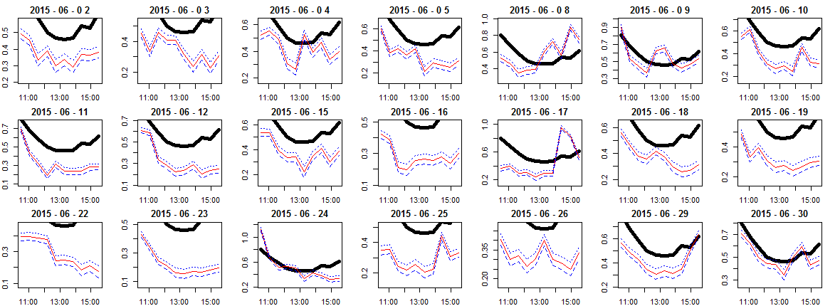
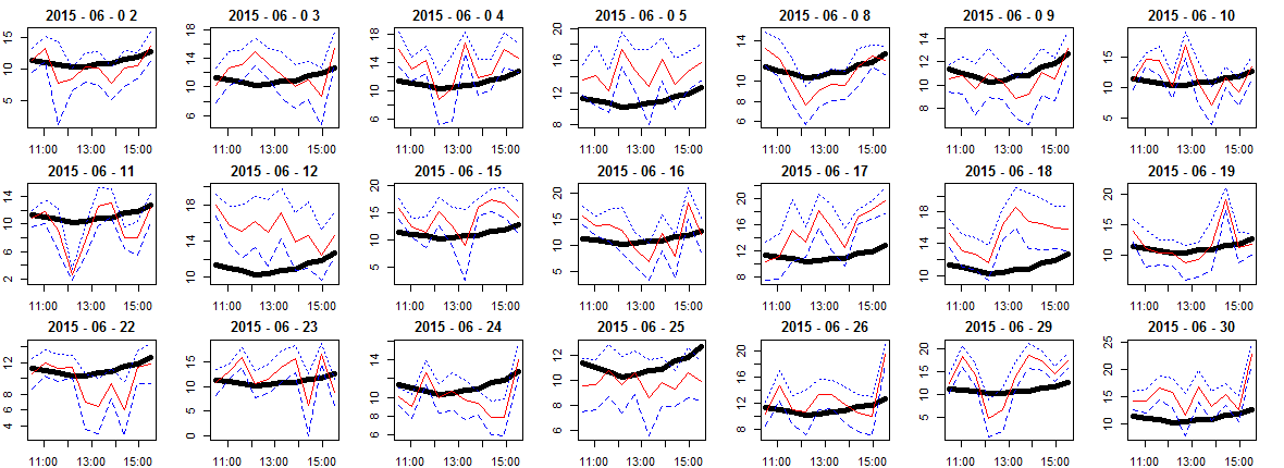
In Figure 2-4, we document the intraday variation of the three parameters. To do that, we divide the 5 hours of trading into 10 blocks of 30 minutes. On each block, we fit the MLE and obtain the corresponding estimates. We also estimate the standard deviation, which allows us to build 95% confidence intervals. Given how volatile the estimates are with respect to their own confidence interval, it is clear that neither the parametric model nor the seasonal component model can be satisfactory to fit such data. This time-varying tendency of parameter intraday values was consistently observed across most of the trading days in 2015. The behavior is heterogeneous in the three parameters. The seasonal model seems to do a decent job for the intensity parameter66 6 probably even better if we add a ”day effect” in the model although the shape of the parameter is very particular for each different day. The seasonal tendency is less clear for the other two parameters. a∗a^{*} tends to oscillate not too far around the seasonal path with a behavior which is day specific, whereas b∗b^{*} can really go far off from one side or the other with no specific pattern. For all those reasons we believe that including in the model both a seasonal and a stochastic effect is more realistic.
Refer to caption
Figure 2: Local estimated ν∗\nu^{*} parameter on 30 minute long blocks in June 2015. The two dashed lines correspond to the 95% confidence intervals. The thick line stands for the seasonality intraday effect, estimated as a temporal local mean across all the trading days in 2015.
Refer to caption
Figure 3: Local estimated a∗a^{*} parameter on 30 minute long blocks in June 2015. The two dashed lines correspond to the 95% confidence intervals. The thick line stands for the seasonality intraday effect, estimated as a temporal local mean across all the trading days in 2015.
Refer to caption
Figure 4: Local estimated b∗b^{*} parameter on 30 minute long blocks in June 2015. The two dashed lines correspond to the 95% confidence intervals. The thick line stands for the seasonality intraday effect, estimated as a temporal local mean across all the trading days in 2015.

In Table 4, we report statistics of the implemented estimators. As our method is non parametric, the assumption of any particular parametric model for the time-varying parameter is not required. Overall we find that the daily estimates are on average roughly equal to (0.56,11,40)(0.56,11,40), with a standard deviation around (0.24,2,8)(0.24,2,8). The results are in line with the numerical study. We implemented five levels of hn=n,2​n,4​n,8​n,h_{n}=\sqrt{n},2\sqrt{n},4\sqrt{n},8\sqrt{n}, 16​n16\sqrt{n} that we denote respectively the corresponding bias-corrected estimators BC 1-5. We can see that BC 2-4 are highly correlated, whereas BC 1 and BC 5 are slightly less correlated. This is probably due to the fact that hnh_{n} can be too small on non active days in the case of BC 1 and too big when considering BC 5. This shows that the local method seems robust to a wide range of possible tuning parameter hnh_{n}. Furthermore, the mean of the MLE and the CH are very different from the one of BC. This is most likely explained by the strong bias obtained in our numerical study. Among those two estimators it is not surprising to find that the MLE is more in line with the local estimates than the CH as the MLE is a "local estimate" in the degenerate case hn=nh_{n}=n.

Table 4: Summary statistics for 12 estimators†
ν∗\nu^{*} a∗a^{*} b∗b^{*}
Est. Mean Stdv. Corr.(,BC 3) Mean Stdv. Corr.(,BC 3) Mean Stdv. Corr.(,BC 3)
naive 1 0.57 0.24 ≈\approx 1 12.48 2.18 0.94 49.80 10.33 0.78
BC 1 0.56 0.24 ≈\approx 1 11.16 2.17 ≈\approx 1 40.24 9.54 0.98
naive 2 0.57 0.24 ≈\approx 1 11.78 2.00 0.98 44.74 8.20 0.89
BC 2 0.56 0.24 ≈\approx 1 11.12 2.00 ≈\approx 1 39.92 7.79 0.99
naive 3 0.56 0.24 ≈\approx 1 11.42 1.96 0.99 42.14 7.58 0.92
BC 3 0.56 0.24 1 11.10 1.96 1 40.16 7.48 1
naive 4 0.56 0.24 ≈\approx 1 11.22 1.96 ≈\approx 1 40.66 7.40 0.96
BC 4 0.56 0.24 ≈\approx 1 11.07 1.96 ≈\approx 1 39.72 7.36 0.94
naive 5 0.56 0.24 ≈\approx 1 11.07 1.97 0.99 39.60 7.50 0.94
BC 5 0.56 0.24 ≈\approx 1 11.01 1.97 0.98 39.14 7.50 0.92
MLE 0.55 0.23 ≈\approx 1 10.78 2.11 0.95 36.77 8.55 0.91
CH 0.55 0.22 0.99 11.69 1.44 0.63 40.50 4.85 0.63

†Sample mean, standard deviation and correlation with BC 3 for the naive estimators (naive 1-5) and the bias-corrected estimators (BC 1-5) with respectively hn=n,2​n,4​n,8​n,16​nh_{n}=\sqrt{n},2\sqrt{n},4\sqrt{n},8\sqrt{n},16\sqrt{n}, the MLE and the CH implemented for APPL in 2015.

9 Conclusion

We have introduced a time-varying parameter extension of the Hawkes process with exponential exciting function. We have also provided an estimator, along with its central limit theorem, of the integrated parameter. We have seen on numerical simulations that this is of particular interest to the practitioner because some concurrent methods (e.g. MLE applied to all the observations) are biased. Finally, our empirical study points out the possible presence of variability in the parameter in addition to seasonal effects.

There are some questions left to explore such as what would happen to the local MLE in the case of a kernel with a fatter tail, such as a polynomial decreasing kernel. As far as the authors know, no convergence of moments of the rescaled MLE has been investigated even in the parametric case. Also, optimality of the tuning parameter hnh_{n} could be investigated, and we could potentially allow for time-varying tuning parameter.

Finally, we point out that the method can be extended to estimate more general key quantities than the integrated parameter, such as functional of the parameter T−1​∫0Tfs​(θs∗)​𝑑sT^{-1}\int_{0}^{T}{f_{s}(\theta_{s}^{*})ds}. In particular, the GCLT for weighted versions T−1​∫0Tθs∗​ws​𝑑sT^{-1}\int_{0}^{T}{\theta_{s}^{*}w_{s}ds} where wsw_{s} is a weight process chosen by the practitioner may be derived by a similar reasoning.

10 Appendix

10.1 The standard MLE for the parametric Hawkes process

We briefly introduce the standard maximum likelihood estimation procedure for the parametric Hawkes process with exponential kernel ϕt=a​e−b​t\phi_{t}=ae^{-bt} in the long run (also called low-frequency) asymptotics, that is when we consider observations of a Hawkes process NPN^{P} on the time interval [0,T][0,T] with T→∞T\to\infty. We define several deterministic key quantities, such as the Fisher information matrix, as time average limits of quantities which depend on the point process NtPN_{t}^{P}.

The regression family is defined for each θ∈K\theta\in K as

λ⁡(t,θ)=ν+∫0t−a​e−b⁡(t−s)​d​NsP.\displaystyle\lambda(t,\theta)=\nu+\int_{0}^{t-}{ae^{-b(t-s)}dN_{s}^{P}}. (10.1)

We assume that there exists an unknown parameter θ∗∈K\theta^{*}\in K such that the ℱtNP{\cal F}_{t}^{N^{P}}-intensity of NtPN_{t}^{P} is expressed as

λ∗P​(t)=λ⁡(t,θ∗).\displaystyle\lambda_{*}^{P}(t)=\lambda(t,\theta^{*}). (10.2)

The log-likelihood process is, up to a constant term,

lT​(θ)=∫0Tlog​(λ⁡(t,θ))​d​NtP−∫0Tλ⁡(t,θ)​𝑑t.\displaystyle l_{T}(\theta)=\int_{0}^{T}{\text{log}\left(\lambda(t,\theta)\right)dN_{t}^{P}}-\int_{0}^{T}{\lambda(t,\theta)dt}. (10.3)

The MLE θ^T\hat{\theta}_{T} is a maximizer of lT​(θ)l_{T}(\theta). We define

ΓT(θ∗)=−1T∂θ2lT(θ∗)∈ℝ3×3,\displaystyle\Gamma_{T}(\theta^{*})=-\frac{1}{T}\partial_{\theta}^{2}l_{T}(\theta^{*})\in\mathbb{R}^{3\times 3}, (10.4)
KT​(θ∗)=1T​∂θ3lT​(θ∗)∈ℝ3×3×3,\displaystyle K_{T}(\theta^{*})=\frac{1}{T}\partial_{\theta}^{3}l_{T}(\theta^{*})\in\mathbb{R}^{3\times 3\times 3}, (10.5)
MT​(θ∗)=∫0T∂θλ⁡(t,θ∗)λ⁡(t,θ∗)​{d​NtP−λ⁡(t,θ∗)​𝑑t},\displaystyle M_{T}(\theta^{*})=\int_{0}^{T}{\frac{\partial_{\theta}\lambda(t,\theta^{*})}{\lambda(t,\theta^{*})}\{dN_{t}^{P}-\lambda(t,\theta^{*})dt\}}, (10.6)

and for any indices k,l,m∈{0,1,2}k,l,m\in\{0,1,2\},

CT​(θ∗)k,l​m=1T​∫0T∂θ,kλ⁡(t,θ∗)​∂θ,l​m2log​(λ⁡(t,θ∗))​𝑑t,\displaystyle C_{T}(\theta^{*})_{k,lm}=\frac{1}{T}\int_{0}^{T}{\partial_{\theta,k}\lambda(t,\theta^{*})\partial_{\theta,lm}^{2}\text{log}\left(\lambda(t,\theta^{*})\right)dt}, (10.7)

and

QT(θ∗)k,l​m=−MT​(θ∗)kT∫0T∂θλ​(t,θ∗)l​∂θλ​(t,θ∗)mλ⁡(t,θ∗)dt.\displaystyle Q_{T}(\theta^{*})_{k,lm}=-\frac{M_{T}(\theta^{*})_{k}}{T}\int_{0}^{T}{\frac{\partial_{\theta}\lambda(t,\theta^{*})_{l}\partial_{\theta}\lambda(t,\theta^{*})_{m}}{\lambda(t,\theta^{*})}dt}. (10.8)

The three time-averaged quantities ΓT\Gamma_{T}, KTK_{T} and CTC_{T} admit deterministic limiting values when T→∞T\to\infty because the process NPN^{P} is exponentially mixing. Indeed, a slight generalization of Lemma 6.6 in [10] shows that the vector process (λ⁡(t,θ∗),∂θ(t,θ∗)CLOSE,(\lambda(t,\theta^{*}),\partial_{\theta}(t,\theta^{*}), OPEN⋯,∂θ3(t,θ∗))\cdots,\partial_{\theta}^{3}(t,\theta^{*})) satisfies the mixing condition [M2] defined on p. 14 in the cited paper, which in turn implies the existence of Γ⁡(θ∗)∈ℝ3×3\Gamma(\theta^{*})\in\mathbb{R}^{3\times 3}, and K⁡(θ∗)K(\theta^{*}), C⁡(θ∗)∈ℝ3×3×3C(\theta^{*})\in\mathbb{R}^{3\times 3\times 3} such that for any ϵ∈(0,1)\epsilon\in(0,1) and any integer p≥1p\geq 1,

𝔼​|ΓT​(θ∗)−Γ⁡(θ∗)|p=O⁡(T−ϵ​p2),\displaystyle\mathbb{E}\left|\Gamma_{T}(\theta^{*})-\Gamma(\theta^{*})\right|^{p}=O\left(T^{-\epsilon\frac{p}{2}}\right), (10.9)
𝔼​|KT​(θ∗)−K⁡(θ∗)|p=O⁡(T−ϵ​p2),\displaystyle\mathbb{E}\left|K_{T}(\theta^{*})-K(\theta^{*})\right|^{p}=O\left(T^{-\epsilon\frac{p}{2}}\right), (10.10)

and

𝔼​|CT​(θ∗)−C⁡(θ∗)|p=O⁡(T−ϵ​p2),\displaystyle\mathbb{E}\left|C_{T}(\theta^{*})-C(\theta^{*})\right|^{p}=O\left(T^{-\epsilon\frac{p}{2}}\right), (10.11)

where |x||x| stands for ∑i|xi|\sum_{i}|x_{i}| for any vector or a matrix xx. Moreover, it is also an easy consequence of the mixing property along with the fact that MT​(θ∗)M_{T}(\theta^{*}) is a martingale that we have the convergence

𝔼⁡[QT​(θ∗)−Q⁡(θ∗)]=O⁡(T−ϵ2),\displaystyle\mathbb{E}\left[Q_{T}(\theta^{*})-Q(\theta^{*})\right]=O\left(T^{-\frac{\epsilon}{2}}\right), (10.12)

for some Q⁡(θ∗)∈ℝ3×3×3Q(\theta^{*})\in\mathbb{R}^{3\times 3\times 3}. Note that Γ⁡(θ∗)\Gamma(\theta^{*}) is the asymptotic Fisher information. In particular, in [10] the authors have shown the convergence of moments of the MLE (see Theorem 4.6),

𝔼⁡[f⁡(T​(θ^T−θ∗))]→𝔼⁡[f⁡(Γ​(θ∗)−12​ξ)],\displaystyle\mathbb{E}\left[f\left(\sqrt{T}(\hat{\theta}_{T}-\theta^{*})\right)\right]\to\mathbb{E}\left[f\left(\Gamma(\theta^{*})^{-\frac{1}{2}}\xi\right)\right], (10.13)

where ff can be any continuous function of polynomial growth, and ξ\xi follows a standard normal distribution. Also, it is easy to see that the convergences in (10.9)-(10.13) hold uniformly in θ∗∈K\theta^{*}\in K under a mild change in the proofs of [10]. The result (10.13) should be compared to Theorem 5.2. Finally, from Γ\Gamma, KK, CC and QQ we define for any k∈{0,1,2}k\in\{0,1,2\}

b​(θ∗)k=12​Γ​(θ∗)j​k​Γ​(θ∗)l​m​(K​(θ∗)j​l​m+2​{C​(θ∗)l,j​m+Q​(θ∗)l,j​m})\displaystyle b(\theta^{*})_{k}=\frac{1}{2}\Gamma(\theta^{*})^{jk}\Gamma(\theta^{*})^{lm}(K(\theta^{*})_{jlm}+2\left\{C(\theta^{*})_{l,jm}+Q(\theta^{*})_{l,jm}\right\}) (10.14)

with implicit summation of repeated indices. The function bb appears in the expression of the expansion of the bias of the local MLE in Section 10.4.

10.2 Construction of the doubly stochastic Hawkes process

We establish the existence of the doubly stochastic self-exciting process under very general conditions on the parameter process. We also provide the boundedness of moments of various stochastic integrals with respect to such point process when the parameter is assumed to take its values in a compact space. We follow the same procedure as in [6] for the construction of a Hawkes process, that is, we show the existence of the doubly stochastic Hawkes process by a fixed point argument. In what follows we let ℬ=(Ω,ℱ,𝐅,ℙ){\cal B}=(\Omega,{\cal F},{\bf F},\mathbb{P}), 𝐅=(ℱt)t∈[0,T]{\bf F}=({\cal F}_{t})_{t\in[0,T]}, ℱ=ℱT{\cal F}={\cal F}_{T} be a stochastic basis such that the filtration 𝐅{\bf F} is generated by the three-dimensional predictable process (θs)s∈[0,T]=(νs,as,bs)s∈[0,T](\theta_{s})_{s\in[0,T]}=(\nu_{s},a_{s},b_{s})_{s\in[0,T]} which is component-wise non-negative, and by a Poisson process N¯\overline{N} of intensity 11 on ℝ2\mathbb{R}^{2} which is independent of θ\theta. In other words, ℱt=ℱt(θ,N¯){\cal F}_{t}={\cal F}_{t}^{(\theta,\overline{N})}. In the following, properties such as predictability or adaptivity will automatically refer to 𝐅{\bf F}. Before we turn to the existence of the self-exciting doubly stochastic process, we recall a key result for martingales.

Lemma 10.1.

Let 𝐅=(ℱt)t∈[0,T],ℱ=ℱT{\bf F}=({\cal F}_{t})_{t\in[0,T]},{\cal F}={\cal F}_{T} be a filtration and 𝒢{\cal G} a σ\sigma-field that is independent of ℱ{\cal F}. Consider also the extended filtration defined by ℋt=ℱt∨𝒢{\cal H}_{t}={\cal F}_{t}\vee{\cal G}. Then any square integrable ℱt{\cal F}_{t}-martingale MM is also a ℋt{\cal H}_{t}-martingale. In particular, for any ℋt{\cal H}_{t}-predictable process uu such that ∫0Tus​d​⟨M,M⟩s\int_{0}^{T}{u_{s}d\langle M,M\rangle_{s}} is integrable, 𝔼⁡[∫0Tus​d​Ms|𝒢]=0\mathbb{E}[\int_{0}^{T}{u_{s}dM_{s}}|{\cal G}]=0.

Proof.

Let MM defined as in the lemma and write for 0≤s≤t≤T0\leq s\leq t\leq T,

𝔼⁡[Mt|ℋs]\displaystyle\mathbb{E}[M_{t}|{\cal H}_{s}] =\displaystyle= 𝔼⁡[Mt|ℱs∨𝒢]\displaystyle\mathbb{E}[M_{t}|{\cal F}_{s}\vee{\cal G}]
=\displaystyle= 𝔼⁡[Mt|ℱs]\displaystyle\mathbb{E}[M_{t}|{\cal F}_{s}]
=\displaystyle= Ms,\displaystyle M_{s},

since 𝒢​⟂⁣⟂⁡Mt{\cal G}\ind M_{t} and 𝒢​⟂⁣⟂⁡ℱs{\cal G}\ind{\cal F}_{s}. It follows that ∫0tus​d​Ms\int_{0}^{t}{u_{s}dM_{s}} is a ℋt{\cal H}_{t}-martingale, the second part of the lemma follows. ∎

We now show the existence of the doubly stochastic Hawkes process associated to θ\theta.

Proof of Theorem 5.1.

We apply a fixed point argument using integrals over the two-dimensional integer measure N¯​(d​t,d​x)\overline{N}(dt,dx). Let us first define λ0​(t)=νt\lambda^{0}(t)=\nu_{t} and N0N^{0} the point process defined as

Nt0=∬[0,t]×ℝ𝟙{0≤x≤λ0(s)}N¯(ds,dx).\displaystyle N_{t}^{0}=\iint_{[0,t]\times\mathbb{R}}{\mathbb{1}_{\{0\leq x\leq\lambda^{0}(s)\}}\overline{N}(ds,dx)}. (10.15)

It is immediate to see that λ0​(t)\lambda^{0}(t) is the ℱt{\cal F}_{t}-intensity of Nt0N_{t}^{0}. We then define recursively the sequence of ℱt{\cal F}_{t}-adapted point processes NnN^{n} along with their stochastic intensities λn\lambda^{n} as

λn+1​(t)\displaystyle\lambda^{n+1}(t) =νt+∫0t−as​e−bs​(t−s)​d​Nsn,\displaystyle=\nu_{t}+\int_{0}^{t-}{a_{s}e^{-b_{s}(t-s)}dN_{s}^{n}}, (10.16a)
Ntn+1\displaystyle N_{t}^{n+1} =∬[0,t]×ℝ𝟙{0≤x≤λn+1(s)}N¯(ds,dx).\displaystyle=\iint_{[0,t]\times\mathbb{R}}{\mathbb{1}_{\{0\leq x\leq\lambda^{n+1}(s)\}}\overline{N}(ds,dx)}. (10.16b)

Note that both λn\lambda^{n} and NnN^{n} are increasing with nn and thus both converge point-wise to some limiting values λ\lambda and NN that take their values on [0,+∞][0,+\infty]. Moreover, NN counts the points of N¯\overline{N} which belong to the positive domain under the curve t↦λ⁡(t)t\mapsto\lambda(t) by an immediate application of the monotone convergence theorem. Let’s now introduce the sequence of processes ρn\rho^{n} defined as ρtn=𝔼[λn(t)−λn−1(t)|ℱTθ]\rho_{t}^{n}=\mathbb{E}\left[\lambda^{n}(t)-\lambda^{n-1}(t)\left|\right.{\cal F}_{T}^{\theta}\right]. Then

ρtn+1\displaystyle\rho_{t}^{n+1} =\displaystyle= 𝔼[∫0tase−bs​(t−s)(λn(s)−λn−1(s))ds|ℱTθ]\displaystyle\mathbb{E}\left[\left.\int_{0}^{t}{a_{s}e^{-b_{s}(t-s)}\left(\lambda^{n}(s)-\lambda^{n-1}(s)\right)ds}\right|{\cal F}_{T}^{\theta}\right]
=\displaystyle= ∫0tase−bs​(t−s)𝔼[λn(s)−λn−1(s)|ℱTθ]ds\displaystyle\int_{0}^{t}{a_{s}e^{-b_{s}(t-s)}\mathbb{E}\left[\left.\lambda^{n}(s)-\lambda^{n-1}(s)\right|{\cal F}_{T}^{\theta}\right]ds}
=\displaystyle= ∫0tas​e−bs​(t−s)​ρsn​𝑑s,\displaystyle\int_{0}^{t}{a_{s}e^{-b_{s}(t-s)}\rho_{s}^{n}ds},

where we used Fubini’s theorem in the second equality. Also, the first equality is obtained by Lemma 10.1 applied to the compensated measure N¯​(d​s,d​z)−d​s⊗d​z\overline{N}(ds,dz)-ds\otimes dz and the independence between ℱTN¯{\cal F}_{T}^{\overline{N}} and ℱTθ{\cal F}_{T}^{\theta}. Thus, setting Φtn=∫0tρsn​𝑑s\Phi_{t}^{n}=\int_{0}^{t}{\rho_{s}^{n}ds}, we have by Fubini’s theorem

Φtn+1=∫0t{∫0t−sas​e−bs​u​𝑑u}​ρsn​𝑑s.\displaystyle\Phi_{t}^{n+1}=\int_{0}^{t}{\left\{\int_{0}^{t-s}{a_{s}e^{-b_{s}u}du}\right\}\rho_{s}^{n}ds}.

Note that ∫0t−sas​e−bs​u​𝑑u≤asbs≤r<1\int_{0}^{t-s}{a_{s}e^{-b_{s}u}du}\leq\frac{a_{s}}{b_{s}}\leq r<1 by condition (5.1). Therefore, Φtn+1≤r​Φtn\Phi_{t}^{n+1}\leq r\Phi_{t}^{n}, and thus the application of the monotone convergence theorem to the sequence (∑k=0nΦtk)n\left(\sum_{k=0}^{n}{\Phi_{t}^{k}}\right)_{n} yields

𝔼[∫0tλ(s)ds|ℱTθ]\displaystyle\mathbb{E}\left[\left.\int_{0}^{t}\lambda(s)ds\right|{\cal F}_{T}^{\theta}\right] ≤\displaystyle\leq ∫0tνsds+r𝔼[∫0tλ(s)ds|ℱTθ].\displaystyle\int_{0}^{t}{\nu_{s}ds}+r\mathbb{E}\left[\left.\int_{0}^{t}\lambda(s)ds\right|{\cal F}_{T}^{\theta}\right]. (10.17)

A straightforward rearrangement of the terms in (10.17) gives us that

𝔼[∫0tλ(s)ds|ℱTθ]≤(1−r)−1∫0tνsds<∞ ℙ−a.s.\mathbb{E}\left[\left.\int_{0}^{t}\lambda(s)ds\right|{\cal F}_{T}^{\theta}\right]\leq(1-r)^{-1}\int_{0}^{t}{\nu_{s}ds}<\infty\text{ }\mathbb{P}-a.s.

where the last inequality is a consequence of condition (5.2). In particular, we deduce that ∫0tλ⁡(s)​𝑑s\int_{0}^{t}\lambda(s)ds and NtN_{t} are both finite almost surely. We need to show that λ⁡(t)\lambda(t) satisfies (5.3). By mononicity, we deduce by taking the limit n→+∞n\to+\infty in (10.16a) that

λ⁡(t)=νt+∫0t−as​e−bs​(t−s)​d​Ns.\displaystyle\lambda(t)=\nu_{t}+\int_{0}^{t-}{a_{s}e^{-b_{s}(t-s)}dN_{s}}. (10.18)

Finally, we show how to obtain (5.4). As N¯\overline{N} and ℱTθ{\cal F}_{T}^{\theta} are independent, it still holds that conditioned on ℱTθ{\cal F}_{T}^{\theta}, N¯\overline{N} is a Poisson process of intensity 11. From the representation of NN as an integral over N¯\overline{N} we conclude that (5.4) holds, and this completes the proof. ∎

We now adapt well-known results on point processes to the case of the doubly stochastic Hawkes process, and derive some useful moments estimates for stochastic integrals with respect to NN. Write Λ¯\overline{\Lambda} the compensating measure of N¯\overline{N}, that is Λ¯​(d​s,d​z)=d​s⊗d​z\overline{\Lambda}(ds,dz)=ds\otimes dz. Given a predictable function WW, write W∗N¯t=∬[0,t]×ℝW⁡(s,z)​N¯​(𝑑s,𝑑z)W\ast\overline{N}_{t}=\iint_{[0,t]\times\mathbb{R}}{W(s,z)\overline{N}(ds,dz)}, and the associated definition for W∗Λ¯tW\ast\overline{\Lambda}_{t}. Predictable function and integral with respect to random measures definitions can be consulted in [27], paragraph II.1. The following lemma is a straightforward adaptation of Lemma I.2.1.5 in [25], using also Lemma 10.1 and (5.4).

Lemma 10.2.

Let WW be a predictable function such that W2∗Λ¯t<∞W^{2}\ast\overline{\Lambda}_{t}<\infty almost surely. Then for any integer p>1p>1, there exists a constant KpK_{p} such that

𝔼[supt∈[0,T]|W∗(N¯−Λ¯)t|p|ℱTθ]\mathbb{E}\left[\left.\sup_{t\in[0,T]}\left|W\ast(\overline{N}-\overline{\Lambda})_{t}\right|^{p}\right|{\cal F}_{T}^{\theta}\right]
≤Kp𝔼[∬[0,T]×ℝ|W(s,z)|pdsdz+(∬[0,T]×ℝW(s,z)2dsdz)p2|ℱTθ]\leq K_{p}\mathbb{E}\left[\iint_{[0,T]\times\mathbb{R}}{|W(s,z)|^{p}}dsdz+\left.\left(\iint_{[0,T]\times\mathbb{R}}{W(s,z)^{2}}dsdz\right)^{\frac{p}{2}}\right|{\cal F}_{T}^{\theta}\right]

For any (random) kernel χ:(s,t)→χ⁡(s,t)\chi:(s,t)\to\chi(s,t), we say that χ\chi is 𝐆{\bf G}-predictable for some filtration 𝐆{\bf G} if for any t∈[0,T]t\in[0,T] the process χ(.,t)\chi(.,t) is. For example the kernel χ⁡(s,t)=as​e−bs​(t−s)\chi(s,t)=a_{s}e^{-b_{s}(t-s)} is 𝐅θ{\bf F}^{\theta}-predictable. Nonetheless, we will also need to deal with other kernels in the course of the proofs. Consequently, we introduce the following lemma, which ensures the boundedness of moments of the doubly stochastic Hawkes process under the condition (5.13).

Lemma 10.3.

Under the condition c:=supt∈[0,T]∫0tase−bs​(t−s)ds<1 ℙ−a.s.c:=\sup_{t\in[0,T]}\int_{0}^{t}{a_{s}e^{-b_{s}(t-s)}ds}<1\text{ }\mathbb{P}-a.s., the counting process NN defined through (5.3) admits moments on [0,T][0,T] that can be bounded by values independent from TT. Moreover, for any 𝐅θ{\bf F}^{\theta}-predictable kernel χ\chi such that ∫0tχ⁡(s,t)​𝑑s\int_{0}^{t}{\chi(s,t)ds} is bounded uniformly in t∈[0,T]t\in[0,T] independently from TT, and for any predictable process ψ\psi that has uniformly bounded moments independently from TT, we have

(i)

supt∈[0,T]𝔼​[λ​(t)p|ℱTθ]1p<Qp\sup_{t\in[0,T]}\mathbb{E}\left[\lambda(t)^{p}|{\cal F}_{T}^{\theta}\right]^{\frac{1}{p}}<Q_{p}

(ii)

supt∈[0,T]𝔼​[(∫0tχ⁡(s,t)​d​Ns)p|ℱTθ]1p<Qp,χ\sup_{t\in[0,T]}\mathbb{E}\left[\left(\int_{0}^{t}{\chi(s,t)dN_{s}}\right)^{p}|{\cal F}_{T}^{\theta}\right]^{\frac{1}{p}}<Q_{p,\chi}

where the constants QpQ_{p}, Qp,χQ_{p,\chi} are independent from TT.

Proof.

We conduct the proof in three steps.

Step 1. We prove that (i) holds for p=1p=1. We write

𝔼⁡[λ⁡(t)|ℱTθ]\displaystyle\mathbb{E}[\lambda(t)|{\cal F}_{T}^{\theta}] =\displaystyle= νt+∫0t−as​e−bs​(t−s)​𝔼​[λ⁡(s)|ℱTθ]​𝑑s\displaystyle\nu_{t}+\int_{0}^{t-}{a_{s}e^{-b_{s}(t-s)}\mathbb{E}[\lambda(s)|{\cal F}_{T}^{\theta}]ds}
≤\displaystyle\leq ν¯+sups∈[0,t]𝔼⁡[λ⁡(s)|ℱTθ]​∫0t−as​e−bs​(t−s)​𝑑s\displaystyle\overline{\nu}+\sup_{s\in[0,t]}\mathbb{E}[\lambda(s)|{\cal F}_{T}^{\theta}]\int_{0}^{t-}{a_{s}e^{-b_{s}(t-s)}ds}
≤\displaystyle\leq ν¯+c​sups∈[0,t]𝔼⁡[λ⁡(s)|ℱTθ],\displaystyle\overline{\nu}+c\sup_{s\in[0,t]}\mathbb{E}[\lambda(s)|{\cal F}_{T}^{\theta}],

where we used condition (5.13) at the last step. Taking the supremum over [0,T][0,T] on both sides, we get

supt∈[0,T]𝔼⁡[λ⁡(t)|ℱTθ]≤(1−c)−1​ν¯.\displaystyle\sup_{t\in[0,T]}\mathbb{E}[\lambda(t)|{\cal F}_{T}^{\theta}]\leq(1-c)^{-1}\overline{\nu}. (10.19)

In particular this proves the case p=1p=1, since the right hand side of (10.19) is independent from TT.

Step 2. We prove that (i) holds for any integer p>1p>1. Note that it is sufficient to consider the case p=2qp=2^{q}, q>0q>0. We thus prove our result by induction on qq. The initialisation case q=0q=0 has been proved in Step 1. Note that for any ϵ>0\epsilon>0,

𝔼⁡[λ​(t)p|ℱTθ]\displaystyle\mathbb{E}[\lambda(t)^{p}|{\cal F}_{T}^{\theta}] ≤\displaystyle\leq (1+ϵ−1)2q−1ν¯+(1+ϵ)2q−1𝔼[(∫0t−ase−bs​(t−s)dNs)p|ℱTθ],\displaystyle(1+\epsilon^{-1})^{2^{q}-1}\overline{\nu}+(1+\epsilon)^{2^{q}-1}\mathbb{E}\left[\left.\left(\int_{0}^{t-}{a_{s}e^{-b_{s}(t-s)}dN_{s}}\right)^{p}\right|{\cal F}_{T}^{\theta}\right],

where we have used the inequality (x+y)2q≤(1+ϵ)2q−1​x2q+(1+ϵ−1)2q−1​y2q(x+y)^{2^{q}}\leq(1+\epsilon)^{2^{q}-1}x^{2^{q}}+(1+\epsilon^{-1})^{2^{q}-1}y^{2^{q}} for any x,y,ϵ>0x,y,\epsilon>0. Now, for a fixed t∈[0,T]t\in[0,T], define W(s,z)=ase−bs​(t−s)𝟙{0≤z≤λ(s)}W(s,z)=a_{s}e^{-b_{s}(t-s)}\mathbb{1}_{\{0\leq z\leq\lambda(s)\}}, and note that

𝔼[(∫0t−ase−bs​(t−s)dNs)p|ℱTθ]\displaystyle\mathbb{E}\left[\left.\left(\int_{0}^{t-}{a_{s}e^{-b_{s}(t-s)}dN_{s}}\right)^{p}\right|{\cal F}_{T}^{\theta}\right] =\displaystyle= 𝔼[(W∗N¯t)p|ℱTθ]\displaystyle\mathbb{E}\left[\left.\left(W\ast\overline{N}_{t}\right)^{p}\right|{\cal F}_{T}^{\theta}\right]
≤\displaystyle\leq (1+ϵ−1)2q−1𝔼[(W∗(N¯−Λ¯)t)p|ℱTθ]\displaystyle(1+\epsilon^{-1})^{2^{q}-1}\mathbb{E}\left[\left.\left(W\ast(\overline{N}-\overline{\Lambda})_{t}\right)^{p}\right|{\cal F}_{T}^{\theta}\right]
+(1+ϵ)2q−1𝔼[(W∗Λ¯t)p|ℱTθ].\displaystyle+(1+\epsilon)^{2^{q}-1}\mathbb{E}\left[\left.\left(W\ast\overline{\Lambda}_{t}\right)^{p}\right|{\cal F}_{T}^{\theta}\right].

We apply now Lemma 10.2 to get

𝔼⁡[(W∗(N¯−Λ¯)t)p|ℱTθ]\displaystyle\mathbb{E}\left[\left(W\ast(\overline{N}-\overline{\Lambda})_{t}\right)^{p}|{\cal F}_{T}^{\theta}\right] ≤\displaystyle\leq Kp𝔼[∬[0,T]×ℝ|W(s,z)|pdsdz+(∬[0,T]×ℝW(s,z)2dsdz)p2|ℱTθ]\displaystyle K_{p}\mathbb{E}\left[\left.\iint_{[0,T]\times\mathbb{R}}{|W(s,z)|^{p}}dsdz+\left(\iint_{[0,T]\times\mathbb{R}}{W(s,z)^{2}}dsdz\right)^{\frac{p}{2}}\right|{\cal F}_{T}^{\theta}\right]
=\displaystyle= Kp𝔼[∫0t−aspe−p​bs​(t−s)λ(s)ds+(∫0t−as2e−2​bs​(t−s)λ(s)ds)p2|ℱTθ].\displaystyle K_{p}\mathbb{E}\left[\left.\int_{0}^{t-}{a_{s}^{p}e^{-pb_{s}(t-s)}\lambda(s)ds}+\left(\int_{0}^{t-}{a_{s}^{2}e^{-2b_{s}(t-s)}\lambda(s)ds}\right)^{\frac{p}{2}}\right|{\cal F}_{T}^{\theta}\right].

We easily bound the first term by the induction hypothesis by some constant Ap2\frac{A_{p}}{2}. For the second term, an elementary application of Hölder’s inequality shows that for any k>1k>1 and any non-negative functions f,gf,g, (∫f​g)k≤(∫fk​g)​(∫g)k−1(\int{fg})^{k}\leq(\int{f^{k}g})(\int{g})^{k-1}. This along with the induction hypothesis leads to a similar bound for the second term. On the other hand, we have

𝔼[(W∗Λ¯t)p|ℱTθ]\displaystyle\mathbb{E}\left[\left.\left(W\ast\overline{\Lambda}_{t}\right)^{p}\right|{\cal F}_{T}^{\theta}\right] =\displaystyle= 𝔼[(∫0t−ase−bs​(t−s)λ(s)ds)p|ℱTθ].\displaystyle\mathbb{E}\left[\left.\left(\int_{0}^{t-}{a_{s}e^{-b_{s}(t-s)}\lambda(s)ds}\right)^{p}\right|{\cal F}_{T}^{\theta}\right].

We apply again the same Hölder’s inequality as above with functions f⁡(s)=λ⁡(s)f(s)=\lambda(s) and g⁡(s)=as​e−bs​(t−s)g(s)=a_{s}e^{-b_{s}(t-s)} to get

𝔼[(∫0t−ase−bs​(t−s)λ(s)ds)p|ℱTθ]\displaystyle\mathbb{E}\left[\left.\left(\int_{0}^{t-}{a_{s}e^{-b_{s}(t-s)}\lambda(s)ds}\right)^{p}\right|{\cal F}_{T}^{\theta}\right] ≤\displaystyle\leq cp−1𝔼[∫0t−ase−bs​(t−s)λ(s)pds|ℱTθ]\displaystyle c^{p-1}\mathbb{E}\left[\left.\int_{0}^{t-}{a_{s}e^{-b_{s}(t-s)}\lambda(s)^{p}ds}\right|{\cal F}_{T}^{\theta}\right]
=\displaystyle= cp−1​∫0t−as​e−bs​(t−s)​𝔼​[λ​(s)p|ℱTθ]​𝑑s\displaystyle c^{p-1}\int_{0}^{t-}{a_{s}e^{-b_{s}(t-s)}\mathbb{E}\left[\lambda(s)^{p}|{\cal F}_{T}^{\theta}\right]ds}
≤\displaystyle\leq cp​sups∈[0,t]𝔼⁡[λ​(s)p|ℱTθ]\displaystyle c^{p}\sup_{s\in[0,t]}{\mathbb{E}\left[\lambda(s)^{p}|{\cal F}_{T}^{\theta}\right]}

Finally, we have shown that

𝔼⁡[λ​(t)p|ℱTθ]\displaystyle\mathbb{E}[\lambda(t)^{p}|{\cal F}_{T}^{\theta}] ≤\displaystyle\leq (1+ϵ−1)2q−1​ν¯+(1+ϵ)2q−1​(1+ϵ−1)2q−1​Ap+(1+ϵ)2q​cp​sups∈[0,t]𝔼⁡[λ​(s)p|ℱTθ].\displaystyle(1+\epsilon^{-1})^{2^{q}-1}\overline{\nu}+(1+\epsilon)^{2^{q}-1}(1+\epsilon^{-1})^{2^{q}-1}A_{p}+(1+\epsilon)^{2^{q}}c^{p}\sup_{s\in[0,t]}\mathbb{E}[\lambda(s)^{p}|{\cal F}_{T}^{\theta}].

This yields, taking supremum over the set [0,T][0,T] and taking ϵ>0\epsilon>0 small enough so that (1+ϵ)2q​cp<1(1+\epsilon)^{2^{q}}c^{p}<1,

supt∈[0,T]𝔼⁡[λ​(t)p|ℱTθ]​(1−(1+ϵ)2q​cp)\displaystyle\sup_{t\in[0,T]}\mathbb{E}[\lambda(t)^{p}|{\cal F}_{T}^{\theta}]\left(1-(1+\epsilon)^{2^{q}}c^{p}\right) ≤\displaystyle\leq (1+ϵ−1)2q−1​ν¯+(1+ϵ)2q−1​(1+ϵ−1)2q−1​Ap,\displaystyle(1+\epsilon^{-1})^{2^{q}-1}\overline{\nu}+(1+\epsilon)^{2^{q}-1}(1+\epsilon^{-1})^{2^{q}-1}A_{p},

and dividing by (1−(1+ϵ)2q​cp)\left(1-(1+\epsilon)^{2^{q}}c^{p}\right) on both sides we get the result.
Step 3. It remains to show (ii) and (iii). But note that they are direct consequences of the boundedness of moments of λ\lambda along with Lemma 10.2.

∎

10.3 LCLT and boundedness of moments of order 2​κ2\kappa

We focus on asymptotic properties of the local maximum likelihood estimator Θ^i,n\widehat{\Theta}_{i,n} of our model on each block i∈{1,⋯,Bn}i\in\{1,\cdots,B_{n}\}. Recall that we are given the global filtration ℱt=ℱt(θ∗,N¯){\cal F}_{t}={\cal F}_{t}^{(\theta^{*},\overline{N})} that bears a sequence of doubly stochastic Hawkes processes (Ntn)t∈[0,T](N_{t}^{n})_{t\in[0,T]}. We perform maximum likelihood estimation on each time block ((i−1)​Δn​T,i​Δn​T]\big((i-1)\Delta_{n}T,i\Delta_{n}T\big], i∈{1,⋯,Bn}i\in\{1,\cdots,B_{n}\} on the regression family of a parametric Hawkes process and show the local central limit theorem for every local estimator Θ^i,n\widehat{\Theta}_{i,n} of θ(i−1)​Δn∗\theta_{(i-1)\Delta_{n}}^{*}, uniformly in the block index ii. In addition, we show that all moments up to order 2​κ>22\kappa>2 of the rescaled estimators hn​(Θ^i,n−θ(i−1)​Δn∗)\sqrt{h_{n}}\big(\widehat{\Theta}_{i,n}-\theta_{(i-1)\Delta_{n}}^{*}\big) are convergent uniformly in ii.

Instead of deriving the limit theorems directly on each block, we show that by a well-chosen time change it is possible to reduce our statistical problem to a long-run framework. Such procedure is based on the following elementary lemma.

Lemma 10.4.

Let (Nt)t(N_{t})_{t} be a point process adapted to a filtration ℱt{\cal F}_{t}, with ℱt{\cal F}_{t}-stochastic intensity λ⁡(t)\lambda(t). For γ>0\gamma>0, consider Ntγ=Nγ​tN_{t}^{\gamma}=N_{\gamma t}, which is adapted to ℱtγ=ℱγ​t{\cal F}_{t}^{\gamma}={\cal F}_{\gamma t}. Then, NtγN_{t}^{\gamma} admits λγ​(t)=γ​λ​(γ​t)\lambda^{\gamma}(t)=\gamma\lambda(\gamma t) as a ℱtγ{\cal F}_{t}^{\gamma}-stochastic intensity. Moreover, if NtN_{t} is a doubly stochastic Hawkes process with parameter process (θs)s(\theta_{s})_{s}, NtγN_{t}^{\gamma} has the distribution of a Hawkes process of parameter (γ​θγ​s)s(\gamma\theta_{\gamma s})_{s}, that is,

λγ​(t)=γ​νγ​t+∫0t−γ​aγ​s​e−γ​bγ​s​(t−s)​d​Nsγ.\displaystyle\lambda^{\gamma}(t)=\gamma\nu_{\gamma t}+\int_{0}^{t-}{\gamma a_{\gamma s}e^{-\gamma b_{\gamma s}(t-s)}dN_{s}^{\gamma}}. (10.20)
Proof.

First note that Ntγ=Nγ​tN_{t}^{\gamma}=N_{\gamma t} is compensated by ∫0γ​tλ⁡(s)​𝑑s\int_{0}^{\gamma t}{\lambda(s)ds}. By a simple change of variable u=γ−1​su=\gamma^{-1}s this integral can be written as ∫0tγ​λ​(γ​u)​𝑑u\int_{0}^{t}{\gamma\lambda(\gamma u)du} which proves the first part of the lemma. In the doubly stochastic Hawkes case, let us write the integral form of the time-changed intensity and apply once again the change of variable u=γ−1​su=\gamma^{-1}s,

λγ​(t)\displaystyle\lambda^{\gamma}(t) =\displaystyle= γ​λ​(γ​t)\displaystyle\gamma\lambda(\gamma t)
=\displaystyle= γ​νγ​t+∫0γ​t−γ​as​e−bs​(γ​t−s)​d​Ns\displaystyle\gamma\nu_{\gamma t}+\int_{0}^{\gamma t-}{\gamma a_{s}e^{-b_{s}(\gamma t-s)}dN_{s}}
=\displaystyle= γ​νγ​t+∫0t−γ​aγ​u​e−γ​bγ​u​(t−u)​d​Nuγ,\displaystyle\gamma\nu_{\gamma t}+\int_{0}^{t-}{\gamma a_{\gamma u}e^{-\gamma b_{\gamma u}(t-u)}dN^{\gamma}_{u}},

and we are done. ∎

By virtue of Lemma 10.4, for any block index i∈{1,⋯,Bn}i\in\{1,\cdots,B_{n}\}, we consider the time change τin:t↦n−1​t+(i−1)​Δn\tau_{i}^{n}:t\mapsto n^{-1}t+(i-1)\Delta_{n} and the point process (Nsn){s∈((i−1)Δn,iΔn]}(N_{s}^{n})_{\{s\in((i-1)\Delta_{n},i\Delta_{n}]\}} in order to get a time changed point process Ni,nN^{i,n} defined on the time set [0,hn​T][0,h_{n}T] by the formula Nti,n=Nτin​(t)n−N(i−1)​ΔnnN_{t}^{i,n}=N_{\tau_{i}^{n}(t)}^{n}-N_{(i-1)\Delta_{n}}^{n}. Such process is adapted to the filtration ℱti,n=ℱτin​(t){\cal F}_{t}^{i,n}={\cal F}_{\tau_{i}^{n}(t)}, for t∈[0,hn​T]t\in[0,h_{n}T]. The parameter processes are now (θti,n,∗){t∈[0,hnT]}=(θτin​(t)∗){t∈[0,hnT]}(\theta_{t}^{i,n,*})_{\{t\in[0,h_{n}T]\}}=(\theta_{\tau_{i}^{n}(t)}^{*})_{\{t\in[0,h_{n}T]\}} whose canonical filtration can be expressed as ℱtθi,n,∗=σ⁡{θsi,n,∗|0≤s≤t}{\cal F}_{t}^{\theta^{i,n,*}}=\sigma\{\theta_{s}^{i,n,*}|0\leq s\leq t\}, for t∈[0,hn​T]t\in[0,h_{n}T]. Finally note that the ℱti,n{\cal F}_{t}^{i,n}-stochastic intensities are now of the form

λ∗i,n​(t)\displaystyle\lambda_{*}^{i,n}(t) =\displaystyle= νti,n,∗+∫0t−asi,n,∗​e−bsi,n,∗​(t−s)​d​Nsi,n+Ri,n​(t),\displaystyle\nu_{t}^{i,n,*}+\int_{0}^{t-}{a_{s}^{i,n,*}e^{-b_{s}^{i,n,*}(t-s)}dN_{s}^{i,n}}+R_{i,n}(t), (10.21)

where Ri,n​(t)R_{i,n}(t) is the ℱ0i,n{\cal F}_{0}^{i,n}-measurable residual process defined by the relation

Ri,n​(t)=∫0(i−1)​Δn−n​as∗​e−n​bs∗​(τin​(t)−s)​d​Nsn.\displaystyle R_{i,n}(t)=\int_{0}^{(i-1)\Delta_{n}-}{na_{s}^{*}e^{-nb_{s}^{*}(\tau_{i}^{n}(t)-s)}dN_{s}^{n}}. (10.22)

Ri,n​(t)R_{i,n}(t) should be interpreted as the pre-excitation induced by the preceding blocks. Note that in view of the exponential form of the kernel ϕt=a​e−b​t\phi_{t}=ae^{-bt} assumption, Ri,n​(t)R_{i,n}(t) can be bounded by

Ri,n​(t)≤e−b¯​t​Ri,n​(0)\displaystyle R_{i,n}(t)\leq e^{-\underline{b}t}R_{i,n}(0) (10.23)

Note that all the processes Ni,nN^{i,n} can be represented as integrals over a sequence of Poisson processes N¯i,n\overline{N}^{i,n} of intensity 11 on ℝ2\mathbb{R}^{2} as follows:

Nti,n=∬[0,t]×ℝ+𝟙{0≤z≤λ∗i,n(s)}N¯i,n(ds,dz).\displaystyle N_{t}^{i,n}=\iint_{[0,t]\times\mathbb{R}_{+}}{\mathbb{1}_{\{0\leq z\leq\lambda_{*}^{i,n}(s)\}}\overline{N}^{i,n}(ds,dz)}. (10.24)

Indeed, N¯i,n\overline{N}^{i,n} is the time-space changed version of the initial Poisson process N¯\overline{N} defined by N¯i,n​(A×B)=N¯​(τin​(A)×n​B)\overline{N}^{i,n}(A\times B)=\overline{N}\left(\tau_{i}^{n}(A)\times nB\right) for AA and BB any two Borel sets of ℝ\mathbb{R}. In the time-changed representation, we define the regression family of stochastic intensities

λ~i,n​(t,θ)=ν+∫0t−a​e−b⁡(t−s)​d​Nsi,n,\displaystyle\tilde{\lambda}^{i,n}(t,\theta)=\nu+\int_{0}^{t-}{ae^{-b(t-s)}dN_{s}^{i,n}}, (10.25)

which is related to λi,n\lambda^{i,n} (see (5.5)) by λ~i,n​(t,θ)=n−1​λi,n​(τin​(t),θ)\tilde{\lambda}^{i,n}(t,\theta)=n^{-1}\lambda^{i,n}(\tau_{i}^{n}(t),\theta). Also, the Quasi Log Likelihood process defined in (5.6) on the ii-th block has now the representation (up to the constant term log​(n)​Nhn​Ti,n\text{log}(n)N_{h_{n}T}^{i,n})

li,n​(θ)=∫0hn​Tlog​(λ~i,n​(t,θ))​d​Nti,n−∫0hn​Tλ~i,n​(t,θ)​𝑑t,\displaystyle l_{i,n}(\theta)=\int_{0}^{h_{n}T}{\text{log}(\tilde{\lambda}^{i,n}(t,\theta))dN_{t}^{i,n}}-\int_{0}^{h_{n}T}{\tilde{\lambda}^{i,n}(t,\theta)dt}, (10.26)

Note that in our case, the true underlying intensity, λ∗i,n\lambda_{*}^{i,n} does not belong to the regression family (λ~i,n(.,θ))θ∈K(\tilde{\lambda}^{i,n}(.,\theta))_{\theta\in K} for two reasons : the parameter process θ∗\theta^{*} is not constant on the ii-th block, and the regression family does not take into account the existence of a pre-excitation term in (10.21). We are in a mispecified case, but we wish to take advantage of the continuity of the process θ∗\theta^{*} to show that the asymptotic theory still holds, that is, the MLE tends to the value θ0i,n,∗=θ(i−1)​Δn∗\theta_{0}^{i,n,*}=\theta_{(i-1)\Delta_{n}}^{*} which is the value of the process θ∗\theta^{*} at the beginning of the ii-th block. The procedure is thus asymptotically equivalent to performing the MLE on the model whose stochastic intensity is in the regression family with true value θ=θ(i−1)​Δn∗\theta=\theta_{(i-1)\Delta_{n}}^{*}. To formalize such idea, we introduce an auxiliary model corresponding to the parametric case generated by the true value θ(i−1)​Δn∗\theta_{(i-1)\Delta_{n}}^{*}. More precisely, we introduce the constant parameter Hawkes process Ni,n,cN^{i,n,c} generated by N¯i,n\overline{N}^{i,n} and the initial value θ0i,n,∗\theta_{0}^{i,n,*}, whose stochastic intensity satisfies

λi,n,c​(t)=ν0i,n,∗+∫0t−a0i,n,∗​e−b0i,n,∗​(t−s)​d​Nsi,n,c.\displaystyle\lambda^{i,n,c}(t)=\nu_{0}^{i,n,*}+\int_{0}^{t-}{a_{0}^{i,n,*}e^{-b_{0}^{i,n,*}(t-s)}dN_{s}^{i,n,c}}. (10.27)

Moreover, we assume that Nti,n,cN_{t}^{i,n,c} has the representation

Nti,n,c=∬[0,t]×ℝ+𝟙{0≤z≤λi,n,c(s)}N¯i,n(ds,dz).\displaystyle N_{t}^{i,n,c}=\iint_{[0,t]\times\mathbb{R}_{+}}{\mathbb{1}_{\{0\leq z\leq\lambda^{i,n,c}(s)\}}\overline{N}^{i,n}(ds,dz)}. (10.28)

Note that Nti,n,cN_{t}^{i,n,c} is unobserved and just used as an intermediary to derive the asymptotic properties of the MLE, by showing systematically that any variable Ni,nN^{i,n}, λ~i,n\tilde{\lambda}^{i,n}, li,nl_{i,n}, etc. is asymptotically very close to its counterpart that is generated by the constant parameter model.

For reasons that will become apparent later, it is crucial to localize the pre-excitation Ri,n​(0)R_{i,n}(0) and bound it by some deterministic value MnM_{n} that depends solely on nn and such that Mn=O⁡(nq)M_{n}=O(n^{q}) for some q>1q>1. To reduce our local estimation problem to the case of a parametric Hawkes process, we will also need to condition with respect to the initial value of the parameter process. We will thus use extensively the conditional expectations 𝔼[.1{Ri,n(0)≤Mn}|ℱ0i,n,θ0i,n,∗=θ0]\mathbb{E}[.\mathbf{1}_{\{R_{i,n}(0)\leq M_{n}\}}|{\cal F}_{0}^{i,n},\theta_{0}^{i,n,*}=\theta_{0}], that we denote by 𝔼θ0,i,n\mathbb{E}_{\theta_{0},i,n}, and whose existences are justified by a classical regular distribution argument77 7 This is a consequence to the fact that K⊂ℝ3K\subset\mathbb{R}^{3} is a Borel space. (see for instance Section 4.34.3 (pp. 77−8077-80) in [5]). In the same spirit, for a measurable set A∈ℱA\in{\cal F}, ℙθ0,i,n​[A]\mathbb{P}_{\theta_{0},i,n}[A] should be understood as 𝔼θ0,i,n​[𝟏A]\mathbb{E}_{\theta_{0},i,n}[\mathbf{1}_{A}]. Finally we will need frequently to take supremum over the quadruplet (θ0,i,n,t)(\theta_{0},i,n,t). For that reason we introduce the notation 𝐄={(θ0,i,n,t)∈K×ℕ2×ℝ+|1≤i≤Bn and 0≤t≤hnT}{\bf E}=\{\left.(\theta_{0},i,n,t)\in K\times\mathbb{N}^{2}\times\mathbb{R}_{+}\right|1\leq i\leq B_{n}\text{ and }0\leq t\leq h_{n}T\}. When n∈ℕn\in\mathbb{N} is fixed, we define 𝐄n{\bf E}_{n} the subset of 𝐄{\bf E} as 𝐄n={(θ0,i,t)∈K×ℕ×ℝ+|1≤i≤Bn and 0≤t≤hnT}{\bf E}_{n}=\{\left.(\theta_{0},i,t)\in K\times\mathbb{N}\times\mathbb{R}_{+}\right|1\leq i\leq B_{n}\text{ and }0\leq t\leq h_{n}T\}. In the same spirit, it is also useful when truncation arguments appear, to consider in the previous equation the subset of 𝐄n{\bf E}_{n} for which we have the stronger condition hnα​T≤t≤hn​Th_{n}^{\alpha}T\leq t\leq h_{n}T where α∈(0,1)\alpha\in(0,1) that we denote by 𝐄nα{\bf E}_{n}^{\alpha}. The next lemma states the uniform boundedness of the moments of λ∗i,n\lambda_{*}^{i,n} and λi,n,c\lambda^{i,n,c}, along with 𝕃p\mathbb{L}^{p} estimates for stochastic integrals over Ni,nN^{i,n} and Ni,n,cN^{i,n,c}.

Lemma 10.5.

We have, for any integer p≥1p\geq 1 and any 𝐅θi,n,∗{\bf F}^{\theta^{i,n,*}}-predictable kernel χ\chi such that ∫0tχ⁡(s,t)​𝑑s\int_{0}^{t}{\chi(s,t)ds} is bounded uniformly in t∈[0,hn​T]t\in[0,h_{n}T] independently from TT and nn,

(i)

sup(θ0,i,n,t)∈𝐄𝔼θ0,i,n|λ∗i,n(t)|p≤Mp ℙ-a.s.\sup_{(\theta_{0},i,n,t)\in{\bf E}}\mathbb{E}_{\theta_{0},i,n}\left|\lambda_{*}^{i,n}(t)\right|^{p}\leq M_{p}\text{ }\mathbb{P}\text{-a.s.}

(ii)

sup(θ0,i,n,t)∈𝐄𝔼θ0,i,n|∫0tχ(s,t)dNsi,n|p<Mp,χ ℙ-a.s.\sup_{(\theta_{0},i,n,t)\in{\bf E}}\mathbb{E}_{\theta_{0},i,n}\left|\int_{0}^{t}{\chi(s,t)dN_{s}^{i,n}}\right|^{p}<M_{p,\chi}\text{ }\mathbb{P}\text{-a.s.}

(iii)

sup(θ0,i,n,t)∈𝐄𝔼θ0,i,n|λi,n,c(t)|p<Mp ℙ-a.s.\sup_{(\theta_{0},i,n,t)\in{\bf E}}\mathbb{E}_{\theta_{0},i,n}\left|\lambda^{i,n,c}(t)\right|^{p}<M_{p}\text{ }\mathbb{P}\text{-a.s.}

(iv)

sup(θ0,i,n,t)∈𝐄𝔼θ0,i,n|∫0tχ(s,t)dNsi,n,c|p<Mp,χ ℙ-a.s.\sup_{(\theta_{0},i,n,t)\in{\bf E}}\mathbb{E}_{\theta_{0},i,n}\left|\int_{0}^{t}{\chi(s,t)dN_{s}^{i,n,c}}\right|^{p}<M_{p,\chi}\text{ }\mathbb{P}\text{-a.s.}

where MpM_{p} and Mp,χM_{p,\chi} are finite constants depending respectively solely on pp and on pp and χ\chi.

Proof.

This is a straightforward adaptation of the proof of Lemma 10.3, with the conditional expectation 𝔼[.1{Ri,n(0)≤Mn}|ℱ0i,n∨ℱhn​Tθi,n,∗,θ0i,n,∗=θ0]\mathbb{E}[.\mathbf{1}_{\{R_{i,n}(0)\leq M_{n}\}}|{\cal F}_{0}^{i,n}\vee{\cal F}_{h_{n}T}^{\theta^{i,n,*}},\theta_{0}^{i,n,*}=\theta_{0}]. The presence of 𝟏{Ri,n(0)≤Mn}\mathbf{1}_{\{R_{i,n}(0)\leq M_{n}\}} along with the exponential decay in (10.23) show clearly that the result still holds, uniformly in the quadruplet (θ0,i,n,t)(\theta_{0},i,n,t). By an immediate application of Jensen’s inequality, this is still true replacing ℱ0i,n∨ℱhn​Tθi,n,∗{\cal F}_{0}^{i,n}\vee{\cal F}_{h_{n}T}^{\theta^{i,n,*}} by the smaller filtration ℱ0i,n{\cal F}_{0}^{i,n}, that is, for the operator 𝔼θ0,i,n\mathbb{E}_{\theta_{0},i,n}. ∎

Before we turn to estimating the distance between the two models, we state a technical lemma.

Lemma 10.6.

Let h:s↦a​e−b​sh:s\mapsto ae^{-bs}, and let ff,gg be two non-negative functions satisfying the inequality f≤g+f∗hf\leq g+f\ast h where (f∗h)​(t)=∫0tf⁡(t−s)​h​(s)​𝑑s(f\ast h)(t)=\int_{0}^{t}{f(t-s)h(s)ds} is the usual convolution. Then we have the majoration for any t≥0t\geq 0

f⁡(t)≤g⁡(t)+a⁡(g∗e(a−b).)​(t)f(t)\leq g(t)+a\left(g\ast e^{(a-b).}\right)(t)
Proof.

Iterating the inequality we get for any n∈ℕ∗n\in\mathbb{N}^{*}

f≤g+g∗∑k=1nh∗(k)+f∗h∗(n+1).\displaystyle f\leq g+g\ast\sum_{k=1}^{n}{h^{\ast(k)}}+f\ast h^{\ast(n+1)}. (10.29)

We fix t≥0t\geq 0, and note that by a straightforward computation, for any integer k≥1k\geq 1 we have h∗(k)​(t)=tk−1(k−1)!​ak​e−b​th^{\ast(k)}(t)=\frac{t^{k-1}}{(k-1)!}a^{k}e^{-bt}. We deduce that

f∗h∗(n+1)​(t)\displaystyle f\ast h^{\ast(n+1)}(t) =\displaystyle= ∫0tf⁡(t−s)​snn!​an+1​e−b​s​𝑑s\displaystyle\int_{0}^{t}{f(t-s)\frac{s^{n}}{n!}a^{n+1}e^{-bs}ds}
≤\displaystyle\leq tnn!​an+1​∫0tf⁡(s)​𝑑s→0\displaystyle\frac{t^{n}}{n!}a^{n+1}\int_{0}^{t}{f(s)ds}\to 0

as n→+∞n\to+\infty. We also have for any integer n≥1n\geq 1

∑k=1nh∗(k)​(t)\displaystyle\sum_{k=1}^{n}{h^{\ast(k)}}(t) =\displaystyle= ∑k=1ntk−1(k−1)!​ak​e−b​t\displaystyle\sum_{k=1}^{n}\frac{t^{k-1}}{(k-1)!}a^{k}e^{-bt}
≤\displaystyle\leq a​e(a−b)​t\displaystyle ae^{(a-b)t}

and thus we get the result by taking the limit n→+∞n\to+\infty in (10.29) evaluated at any point t≥0t\geq 0. ∎

In what follows, we quantify the local error between the doubly stochastic model and its constant parameter approximation. We recall the value of the key exponent κ=γ⁡(δ−1)\kappa=\gamma(\delta-1) that has been introduced in (5.16), and which plays an important role in the next results as it proves to be the rate of convergence of one model to the other in power of hn−1h_{n}^{-1}, where hnh_{n} is proportional to the typical size of one block after our time change. Recall that γ\gamma represents the regularity exponent in time of θ\theta while δ\delta controls the size of small blocks compared to nn by the relation hn=n1/δh_{n}=n^{1/\delta}. Note that by (5.16) we have κ>1\kappa>1. The next lemma shows that the models (Ni,n,c,λi,n,c)(N^{i,n,c},\lambda^{i,n,c}) and (Ni,n,λ∗i,n)(N^{i,n},\lambda_{*}^{i,n}) are asymptotically close in the 𝕃p\mathbb{L}^{p} sense. The proof follows the same path as the proof of Lemma 10.3.

Lemma 10.7.

Let α∈(0,1)\alpha\in(0,1) be a truncation exponent, and ϵ∈(0,1)\epsilon\in(0,1). We have, for any p≥1p\geq 1, any deterministic kernel χ\chi such that ∫0tχ⁡(s,t)​𝑑s\int_{0}^{t}{\chi(s,t)ds} is bounded uniformly in t∈ℝ+t\in\mathbb{R}_{+}, and any predictable process (ψs)s∈ℝ+\left(\psi_{s}\right)_{s\in\mathbb{R}_{+}} whose moments are bounded :

(i)

sup(θ0,i,t)∈𝐄nα𝔼θ0,i,n​|λi,n,c​(t)−λ∗i,n​(t)|p=Oℙ​(hn−κ)\sup_{(\theta_{0},i,t)\in{\bf E}_{n}^{\alpha}}\mathbb{E}_{\theta_{0},i,n}\left|\lambda^{i,n,c}(t)-\lambda_{*}^{i,n}(t)\right|^{p}=O_{\mathbb{P}}\left(h_{n}^{-\kappa}\right)

(ii)

supθ0∈K,1≤i≤Bn𝔼θ0,i,n​|∫hnα​Thn​Tψs​{d​Nsi,n,c−d​Nsi,n}|p=Oℙ​(hnp−ϵ​κ)\sup_{\theta_{0}\in K,1\leq i\leq B_{n}}\mathbb{E}_{\theta_{0},i,n}\left|\int_{h_{n}^{\alpha}T}^{h_{n}T}{\psi_{s}\{dN_{s}^{i,n,c}-dN_{s}^{i,n}\}}\right|^{p}=O_{\mathbb{P}}\left(h_{n}^{p-\epsilon\kappa}\right)

(iii)

supθ0∈K,1≤i≤Bn𝔼θ0,i,n​|∫hnα​Thn​Tχ⁡(s,hn​T)​{d​Nsi,n,c−d​Nsi,n}|p=Oℙ​(hn−κ)\sup_{\theta_{0}\in K,1\leq i\leq B_{n}}\mathbb{E}_{\theta_{0},i,n}\left|\int_{h_{n}^{\alpha}T}^{h_{n}T}{\chi(s,h_{n}T)\{dN_{s}^{i,n,c}-dN_{s}^{i,n}\}}\right|^{p}=O_{\mathbb{P}}\left(h_{n}^{-\kappa}\right)

Remark 10.8.

For p=1p=1, if we recall that Δn=hn​n−1​T\Delta_{n}=h_{n}n^{-1}T and κ=γ⁡(δ−1)\kappa=\gamma(\delta-1), we get a typical deviation in hn−κ=T−γ​Δnγh_{n}^{-\kappa}=T^{-\gamma}\Delta_{n}^{\gamma} between the real model and its constant parameter approximation. This is not very surprising since on one block the parameter process θ∗\theta^{*} has exactly a deviation of that order. For p>1p>1, the situation is fairly different. One would expect a deviation of the same order of that of the parameter process, that is of order hn−κ​p=T−γ​p​Δnγ​ph_{n}^{-\kappa p}=T^{-\gamma p}\Delta_{n}^{\gamma p}. But as it is shown in the previous lemma, deviations between the two models are quite weaker since the deviation remains of order hn−κ=T−γ​Δnγh_{n}^{-\kappa}=T^{-\gamma}\Delta_{n}^{\gamma} for any pp. This loss is due to the point process structure and the shape of its related Burkholder-Davis-Gundy type inequality (see Lemma 10.2). This is the same phenomenon as in the following fact. For a Poisson process NN of intensity λ\lambda, we have 𝔼⁡[|Nt−λ​t|p]∼αp​t\mathbb{E}[|N_{t}-\lambda t|^{p}]\sim\alpha_{p}t when t→0t\to 0, i.e. a rate of convergence which is linear regardless of the moment chosen.

Proof.

We will show by recurrence on q∈ℕq\in\mathbb{N} that for every pp of the form p=2qp=2^{q}, we have the majoration for n∈ℕn\in\mathbb{N}, t∈[0,hn​T]t\in[0,h_{n}T] and uniformly in (θ0,i)(\theta_{0},i),

𝔼θ0,i,n​|λi,n,c​(t)−λ∗i,n​(t)|2q≤Ln,q+Mn,q​e−b¯​(1−r)​t,\displaystyle\mathbb{E}_{\theta_{0},i,n}\left|\lambda^{i,n,c}(t)-\lambda_{*}^{i,n}(t)\right|^{2^{q}}\leq L_{n,q}+M_{n,q}e^{-\underline{b}(1-r)t}, (10.30)

where Ln,qL_{n,q} and Mn,qM_{n,q} depend on nn and qq only, Ln,q=Oℙ​(hn−κ)L_{n,q}=O_{\mathbb{P}}(h_{n}^{-\kappa}), and Mn,qM_{n,q} is of polynomial growth in nn. Note that then (i) will be automatically proved since by taking the supremum over the set [hnα​T,hn​T][h_{n}^{\alpha}T,h_{n}T] and using the estimate Mn,q​e−b¯​(1−r)​hnα​T=oℙ​(hn−κ)M_{n,q}e^{-\underline{b}(1-r)h_{n}^{\alpha}T}=o_{\mathbb{P}}(h_{n}^{-\kappa}) we get

𝔼θ0,i,n​|λn,c​(t)−λ∗n​(t)|p=Oℙ​(hn−κ)\mathbb{E}_{\theta_{0},i,n}|\lambda^{n,c}(t)-\lambda_{*}^{n}(t)|^{p}=O_{\mathbb{P}}(h_{n}^{-\kappa})

uniformly over the set 𝐄nα{\bf E}_{n}^{\alpha}.

Step 1. We show our claim in the case q=0q=0, that is p=1p=1. Write

|λ∗i,n​(t)−λi,n,c​(t)|\displaystyle|\lambda_{*}^{i,n}(t)-\lambda^{i,n,c}(t)| ≤\displaystyle\leq |νti,n,∗−ν0i,n,∗|+|∫0t−(asi,n,∗​e−bsi,n,∗​(t−s)−a0i,n,∗​e−b0i,n,∗​(t−s))​d​Nsi,n|\displaystyle|\nu_{t}^{i,n,*}-\nu_{0}^{i,n,*}|+\left|\int_{0}^{t-}{\left(a_{s}^{i,n,*}e^{-b_{s}^{i,n,*}(t-s)}-a_{0}^{i,n,*}e^{-b_{0}^{i,n,*}(t-s)}\right)}dN_{s}^{i,n}\right|
+\displaystyle+ |∫0t−a0i,n,∗​e−b0i,n,∗​(t−s)​(d​Nsi,n,c−d​Nsi,n)|+Ri,n​(t)\displaystyle\left|\int_{0}^{t-}{a_{0}^{i,n,*}e^{-b_{0}^{i,n,*}(t-s)}\left(dN_{s}^{i,n,c}-dN_{s}^{i,n}\right)}\right|+R_{i,n}(t)
≤\displaystyle\leq Ai,n​(t)+Bi,n​(t)+Ci,n​(t)+Ri,n​(t)\displaystyle A_{i,n}(t)+B_{i,n}(t)+C_{i,n}(t)+R_{i,n}(t)

The (uniform) majoration 𝔼θ0,i,n​Ai,n​(t)=Oℙ​(hn−κ)\mathbb{E}_{\theta_{0},i,n}A_{i,n}(t)=O_{\mathbb{P}}(h_{n}^{-\kappa}) is an immediate consequence of [C]-(i). By the inequality

|ae−b​t−a′e−b′t|≤(|a−a′|+|b−b′|)e−b¯​t\displaystyle|ae^{-bt}-a^{{}^{\prime}}e^{-b^{{}^{\prime}}t}|\leq\left(|a-a^{{}^{\prime}}|+|b-b^{{}^{\prime}}|\right)e^{-\underline{b}t} (10.31)

for any (ν,a,b),(ν′,a′,b′)∈K(\nu,a,b),(\nu^{{}^{\prime}},a^{{}^{\prime}},b^{{}^{\prime}})\in K, we can write

𝔼θ0,i,n​Bi,n​(t)\displaystyle\mathbb{E}_{\theta_{0},i,n}B_{i,n}(t) ≤\displaystyle\leq 𝔼θ0,i,n​∫0t−(|asi,n,∗−a0|+|bsi,n,∗−b0|)​e−b¯​(t−s)​d​Nsi,n\displaystyle\mathbb{E}_{\theta_{0},i,n}\int_{0}^{t-}{\left(|a_{s}^{i,n,*}-a_{0}|+|b_{s}^{i,n,*}-b_{0}|\right)e^{-\underline{b}(t-s)}dN_{s}^{i,n}}
≤\displaystyle\leq 𝔼θ0,i,n​|sups∈[0,t](|asi,n,∗−a0|+|bsi,n,∗−b0|)|2​𝔼θ0,i,n​|∫0t−e−b¯​(t−s)​d​Nsi,n|2,\displaystyle\sqrt{\mathbb{E}_{\theta_{0},i,n}\left|\sup_{s\in[0,t]}{\left(|a_{s}^{i,n,*}-a_{0}|+|b_{s}^{i,n,*}-b_{0}|\right)}\right|^{2}\mathbb{E}_{\theta_{0},i,n}\left|\int_{0}^{t-}{e^{-\underline{b}(t-s)}dN_{s}^{i,n}}\right|^{2}},

where Cauchy-Schwartz inequality was applied in the last inequality. Note that the right term is almost surely dominated by a constant by Lemma 10.5 and thus the uniform majoration 𝔼θ0,i,n​Bi,n​(t)=Oℙ​(hn−κ)\mathbb{E}_{\theta_{0},i,n}B_{i,n}(t)=O_{\mathbb{P}}(h_{n}^{-\kappa}) follows from [C]-(i). Finally, for Ci,n​(t)C_{i,n}(t), write

𝔼θ0,i,n​Ci,n​(t)\displaystyle\mathbb{E}_{\theta_{0},i,n}C_{i,n}(t) ≤\displaystyle\leq 𝔼θ0,i,n​∫0t−a0​e−b0​(t−s)​d​|Ni,n,c−Ni,n|s\displaystyle\mathbb{E}_{\theta_{0},i,n}\int_{0}^{t-}{a_{0}e^{-b_{0}(t-s)}d\left|N^{i,n,c}-N^{i,n}\right|_{s}} (10.32)

where d​|Ni,n,c−Ni,n|sd\left|N^{i,n,c}-N^{i,n}\right|_{s} is the integer measure which counts the jumps that don’t belong to both d​Ni,n,cdN^{i,n,c} and d​Ni,ndN^{i,n}, i.e. the points of N¯i,n\overline{N}^{i,n} that lay between the curves t→λ∗i,n​(t)t\to\lambda_{*}^{i,n}(t) and t→λi,n,c​(t)t\to\lambda^{i,n,c}(t). A short calculation shows that this counting process admits |λi,n,c​(s)−λ∗i,n​(s)||\lambda^{i,n,c}(s)-\lambda_{*}^{i,n}(s)| as stochastic intensity. We compute now:

𝔼θ0,i,n​Ci,n​(t)\displaystyle\mathbb{E}_{\theta_{0},i,n}C_{i,n}(t) ≤\displaystyle\leq 𝔼θ0,i,n​∫0t−a0​e−b0​(t−s)​|λi,n,c​(s)−λ∗i,n​(s)|​𝑑s\displaystyle\mathbb{E}_{\theta_{0},i,n}\int_{0}^{t-}{a_{0}e^{-b_{0}(t-s)}|\lambda^{i,n,c}(s)-\lambda_{*}^{i,n}(s)|ds}
=\displaystyle= ∫0t−a0​e−b0​(t−s)​𝔼θ0,i,n​|λi,n,c​(s)−λ∗i,n​(s)|​𝑑s.\displaystyle\int_{0}^{t-}{a_{0}e^{-b_{0}(t-s)}\mathbb{E}_{\theta_{0},i,n}|\lambda^{i,n,c}(s)-\lambda_{*}^{i,n}(s)|ds}.

So far we have shown that there exists a sequence LnL_{n} such that Ln=O⁡(hn−κ)L_{n}=O(h_{n}^{-\kappa}) and such that the function f⁡(t)=𝔼θ0,i,n​|λi,n,c​(t)−λ∗i,n​(t)|f(t)=\mathbb{E}_{\theta_{0},i,n}|\lambda^{i,n,c}(t)-\lambda_{*}^{i,n}(t)| satisfies the inequality

f⁡(t)≤Ln+Ri,n​(t)+f∗h⁡(t),\displaystyle f(t)\leq L_{n}+R_{i,n}(t)+f\ast h(t), (10.33)

where hh is the kernel defined as h:t↦a0​e−b0​th:t\mapsto a_{0}e^{-b_{0}t}. By Lemma 10.6, this yields

f⁡(t)≤Ln+Ri,n​(t)+∫0t{Ln+Ri,n​(s)}​a0​e(a0−b0)​(t−s)​𝑑s.\displaystyle f(t)\leq L_{n}+R_{i,n}(t)+\int_{0}^{t}{\{L_{n}+R_{i,n}(s)\}a_{0}e^{(a_{0}-b_{0})(t-s)}ds}. (10.34)

Now recall that b0−a0>b¯​(1−r)b_{0}-a_{0}>\underline{b}(1-r) and that on the set {Ri,n(0)≤Mn}\{R_{i,n}(0)\leq M_{n}\}, we have Ri,n​(s)≤Mn​e−b¯​s<Mn​e−b¯​(1−r)​sR_{i,n}(s)\leq M_{n}e^{-\underline{b}s}<M_{n}e^{-\underline{b}(1-r)s} to get

f⁡(t)\displaystyle f(t) ≤\displaystyle\leq (1+(1−r)−1)​Ln+Ri,n​(t)+∫0t{Mn​e−b¯​(1−r)​s}​a0​eb¯​(1−r)​(t−s)​𝑑s\displaystyle(1+(1-r)^{-1})L_{n}+R_{i,n}(t)+\int_{0}^{t}{\{M_{n}e^{-\underline{b}(1-r)s}\}a_{0}e^{\underline{b}(1-r)(t-s)}ds}
≤\displaystyle\leq (1+(1−r)−1)​Ln+(1+a¯​t)​Mn​e−b¯​(1−r)​t.\displaystyle(1+(1-r)^{-1})L_{n}+(1+\overline{a}t)M_{n}e^{-\underline{b}(1-r)t}.

If we recall that in the above expression f⁡(t)f(t) stands for 𝔼θ0,i,n​|λi,n,c​(t)−λ∗i,n​(t)|\mathbb{E}_{\theta_{0},i,n}|\lambda^{i,n,c}(t)-\lambda_{*}^{i,n}(t)|, such uniform estimate clearly proves (10.30) in the case q=1q=1.

Step 2. We prove the result for any q∈ℕ∗q\in\mathbb{N}^{*}. Let the expression f⁡(t)f(t) stands for 𝔼θ0,i,n​|λi,n,c​(t)−λ∗i,n​(t)|p\mathbb{E}_{\theta_{0},i,n}|\lambda^{i,n,c}(t)-\lambda_{*}^{i,n}(t)|^{p}. With similar notations as for the previous step, we have for any η>0\eta>0

f⁡(t)=𝔼θ0,i,n​|λi,n,c​(t)−λ∗i,n​(t)|p\displaystyle f(t)=\mathbb{E}_{\theta_{0},i,n}|\lambda^{i,n,c}(t)-\lambda_{*}^{i,n}(t)|^{p} ≤\displaystyle\leq 𝔼θ0,i,n​|Ai,n​(t)+Bi,n​(t)+Ci,n​(t)+Ri,n​(t)|p\displaystyle\mathbb{E}_{\theta_{0},i,n}\left|A_{i,n}(t)+B_{i,n}(t)+C_{i,n}(t)+R_{i,n}(t)\right|^{p}
≤\displaystyle\leq (1+η−1)2q−1​𝔼θ0,i,n​|Ai,n​(t)+Bi,n​(t)+Ri,n​(t)|p\displaystyle(1+\eta^{-1})^{2^{q}-1}\mathbb{E}_{\theta_{0},i,n}\left|A_{i,n}(t)+B_{i,n}(t)+R_{i,n}(t)\right|^{p}
+(1+η)2q−1​𝔼θ0,i,n​Ci,n​(t)p\displaystyle+(1+\eta)^{2^{q}-1}\mathbb{E}_{\theta_{0},i,n}C_{i,n}(t)^{p}

It is straightforward to see that similar arguments to the previous case lead to the uniform estimate

𝔼θ0,i,n​Ai,n​(t)p+𝔼θ0,i,n​Bi,n​(t)p=Oℙ​(hn−κ​p).\displaystyle\mathbb{E}_{\theta_{0},i,n}A_{i,n}(t)^{p}+\mathbb{E}_{\theta_{0},i,n}B_{i,n}(t)^{p}=O_{\mathbb{P}}\left(h_{n}^{-\kappa p}\right).

Now, define W(s,z)=a0e−b0​(t−s)|𝟙{0≤z≤λi,n,c(s)}−𝟙{0≤z≤λ∗i,n(s)}|W(s,z)=a_{0}e^{-b_{0}(t-s)}|\mathbb{1}_{\{0\leq z\leq\lambda^{i,n,c}(s)\}}-\mathbb{1}_{\{0\leq z\leq\lambda_{*}^{i,n}(s)\}}| to get

𝔼θ0,i,n​[Ci,n​(t)p]\displaystyle\mathbb{E}_{\theta_{0},i,n}\left[C_{i,n}(t)^{p}\right] =\displaystyle= 𝔼θ0,i,n​[(W∗N¯t)p]\displaystyle\mathbb{E}_{\theta_{0},i,n}\left[\left(W\ast\overline{N}_{t}\right)^{p}\right]
≤\displaystyle\leq (1+η−1)2q−1​𝔼θ0,i,n​[(W∗(N¯−Λ¯)t)p]+(1+η)2q−1​𝔼θ0,i,n​[(W∗Λ¯t)p],\displaystyle(1+\eta^{-1})^{2^{q}-1}\mathbb{E}_{\theta_{0},i,n}\left[\left(W\ast(\overline{N}-\overline{\Lambda})_{t}\right)^{p}\right]+(1+\eta)^{2^{q}-1}\mathbb{E}_{\theta_{0},i,n}\left[\left(W\ast\overline{\Lambda}_{t}\right)^{p}\right],

and apply Lemma 10.2 to get

𝔼θ0,i,n​[(W∗(N¯−Λ¯)t)p]\displaystyle\mathbb{E}_{\theta_{0},i,n}\left[\left(W\ast(\overline{N}-\overline{\Lambda})_{t}\right)^{p}\right] ≤\displaystyle\leq Kp​(𝔼θ0,i,n​[∬[0,T]×ℝ|W⁡(s,z)|p​𝑑s​𝑑z]CLOSE\displaystyle K_{p}\left(\mathbb{E}_{\theta_{0},i,n}\left[\iint_{[0,T]\times\mathbb{R}}{|W(s,z)|^{p}}dsdz\right]\right.
OPEN+𝔼θ0,i,n​[(∬[0,T]×ℝW​(s,z)2​𝑑s​𝑑z)p2])\displaystyle+\left.\mathbb{E}_{\theta_{0},i,n}\left[\left(\iint_{[0,T]\times\mathbb{R}}{W(s,z)^{2}}dsdz\right)^{\frac{p}{2}}\right]\right)
=\displaystyle= Kp​(𝔼θ0,i,n​[∫0t−a0p​e−p​b0​(t−s)​|λi,n,c​(s)−λ∗i,n​(s)|​𝑑s]CLOSE\displaystyle K_{p}\left(\mathbb{E}_{\theta_{0},i,n}\left[\int_{0}^{t-}{a_{0}^{p}e^{-pb_{0}(t-s)}|\lambda^{i,n,c}(s)-\lambda_{*}^{i,n}(s)|ds}\right]\right.
OPEN+𝔼θ0,i,n​[(∫0t−a02​e−2​b0​(t−s)​|λi,n,c​(s)−λ∗i,n​(s)|​𝑑s)p2]),\displaystyle+\left.\mathbb{E}_{\theta_{0},i,n}\left[\left(\int_{0}^{t-}{a_{0}^{2}e^{-2b_{0}(t-s)}|\lambda^{i,n,c}(s)-\lambda_{*}^{i,n}(s)|ds}\right)^{\frac{p}{2}}\right]\right),

which is easily bounded as in (10.30) using the induction hypothesis. Note that here the presence of the integral term in |λi,n,c​(s)−λ∗i,n​(s)||\lambda^{i,n,c}(s)-\lambda_{*}^{i,n}(s)| is the major obstacle to getting the stronger estimate Oℙ​(hn−κ​p)O_{\mathbb{P}}\left(h_{n}^{-\kappa p}\right) that one would expect. Finally the term

𝔼θ0,i,n​[(W∗Λ¯t)p]=𝔼θ0,i,n​[(∫0t−a0​e−b0​(t−s)​|λi,n,c​(s)−λ∗i,n​(s)|​𝑑s)p]\mathbb{E}_{\theta_{0},i,n}\left[\left(W\ast\overline{\Lambda}_{t}\right)^{p}\right]=\mathbb{E}_{\theta_{0},i,n}\left[\left(\int_{0}^{t-}{a_{0}e^{-b_{0}(t-s)}|\lambda^{i,n,c}(s)-\lambda_{*}^{i,n}(s)|ds}\right)^{p}\right]

is treated exactly in the same way as for the proof of Lemma 10.3, to get the bound

𝔼θ0,i,n​[(W∗Λ¯t)p]\displaystyle\mathbb{E}_{\theta_{0},i,n}\left[\left(W\ast\overline{\Lambda}_{t}\right)^{p}\right] ≤\displaystyle\leq cq​f∗h⁡(t),\displaystyle c_{q}f\ast h(t), (10.35)

where again h:s↦a0​e−b0​sh:s\mapsto a_{0}e^{-b_{0}s}, and cq<1c_{q}<1 if η\eta is taken small enough. We have thus shown that ff satisfies a similar convolution inequality as for the case q=1q=1 and we can apply Lemma 10.6 to conclude.

Step 3. It remains to show (ii) and (iii). They are just consequences of the application of Lemma 10.2 to the case Wψ(s,z)=ψs|𝟙{0≤z≤λn,c(s)}−𝟙{0≤z≤λ∗n(s)}|W_{\psi}(s,z)=\psi_{s}|\mathbb{1}_{\{0\leq z\leq\lambda^{n,c}(s)\}}-\mathbb{1}_{\{0\leq z\leq\lambda_{*}^{n}(s)\}}| and Wχ(s,z)=χ(s,t)|𝟙{0≤z≤λn,c(s)}−𝟙{0≤z≤λ∗n(s)}|W_{\chi}(s,z)=\chi(s,t)|\mathbb{1}_{\{0\leq z\leq\lambda^{n,c}(s)\}}-\mathbb{1}_{\{0\leq z\leq\lambda_{*}^{n}(s)\}}| along with Hölder’s inequality. ∎

We are now ready to show the uniform asymptotic normality of the MLE by proving that any quantity related to the estimation is asymptotically very close to its counterpart for the constant parameter model (Ni,n,c,λi,n,c)(N^{i,n,c},\lambda^{i,n,c}). To this end we introduce the fake candidate intensity family and the fake log-likelihood process, as

λi,n,c​(t,θ)=ν+∫0t−a​e−b⁡(t−s)​d​Nsi,n,c\displaystyle\lambda^{i,n,c}(t,\theta)=\nu+\int_{0}^{t-}{ae^{-b(t-s)}dN_{s}^{i,n,c}} (10.36)

and

li,nc​(θ)=∫0hn​Tlog​(λi,n,c​(t,θ))​d​Nti,n,c−∫0hn​Tλi,n,c​(t,θ)​𝑑t,\displaystyle l_{i,n}^{c}(\theta)=\int_{0}^{h_{n}T}{\text{log}(\lambda^{i,n,c}(t,\theta))dN_{t}^{i,n,c}}-\int_{0}^{h_{n}T}{\lambda^{i,n,c}(t,\theta)dt}, (10.37)

for any θ∈K\theta\in K. Note that λi,n,c​(t,θ0i,n,∗)=λi,n,c​(t)\lambda^{i,n,c}(t,\theta_{0}^{i,n,*})=\lambda^{i,n,c}(t) by definition. Those quantities, which are all related to (Ni,n,c,λi,n,c)(N^{i,n,c},\lambda^{i,n,c}), are unobserved.

As a consequence of the previous lemma we state the uniform 𝕃p\mathbb{L}^{p} boundedness of the candidate intensity families, along with estimates of their relative deviations.

Lemma 10.9.

Let α∈(0,1)\alpha\in(0,1). We have for any integer p≥1p\geq 1 and any j∈ℕj\in\mathbb{N} that

(i)

sup(θ0,i,n,t)∈𝐄𝔼θ0,i,nsupθ∈K|∂θjλ~i,n(t,θ)|p≤Kj ℙ-a.s.\sup_{(\theta_{0},i,n,t)\in{\bf E}}\mathbb{E}_{\theta_{0},i,n}\sup_{\theta\in K}\left|\partial_{\theta}^{j}\tilde{\lambda}^{i,n}(t,\theta)\right|^{p}\leq K_{j}\text{ }\mathbb{P}\text{-a.s.}

(ii)

sup(θ0,i,n,t)∈𝐄𝔼θ0,i,nsupθ∈K|∂θjλi,n,c(t,θ)|p≤Kj ℙ-a.s.\sup_{(\theta_{0},i,n,t)\in{\bf E}}\mathbb{E}_{\theta_{0},i,n}\sup_{\theta\in K}\left|\partial_{\theta}^{j}\lambda^{i,n,c}(t,\theta)\right|^{p}\leq K_{j}\text{ }\mathbb{P}\text{-a.s.}

(iii)

sup(θ0,i,t)∈𝐄nα𝔼θ0,i,n​supθ∈K|∂θjλ~i,n​(t,θ)−∂θjλi,n,c​(t,θ)|p=Oℙ​(hn−κ)\sup_{(\theta_{0},i,t)\in{\bf E}_{n}^{\alpha}}\mathbb{E}_{\theta_{0},i,n}\sup_{\theta\in K}\left|\partial_{\theta}^{j}\tilde{\lambda}^{i,n}(t,\theta)-\partial_{\theta}^{j}\lambda^{i,n,c}(t,\theta)\right|^{p}=O_{\mathbb{P}}(h_{n}^{-\kappa})

where the constants KjK_{j} depend solely on jj.

Proof.

Note that the derivatives of λ~i,n​(t,θ)\tilde{\lambda}^{i,n}(t,\theta) can be all bounded uniformly in θ\theta by linear combinations of terms of the form ν¯\overline{\nu} or ∫0t−(t−s)j​e−b¯​(t−s)​d​Nsi,n\int_{0}^{t-}{(t-s)^{j}e^{-\underline{b}(t-s)}dN_{s}^{i,n}}, j∈ℕj\in\mathbb{N}. The boundedness of moments of those terms uniformly in n∈ℕn\in\mathbb{N} and in the time interval [0,hn​T][0,h_{n}T] is thus the consequence of Lemma 10.3 (ii) with χ⁡(s,t)=(t−s)j​e−b¯​(t−s)\chi(s,t)=(t-s)^{j}e^{-\underline{b}(t-s)}, and consequently (i) follows. (ii) is proved in the same way. Finally we show (iii). Note that supθ∈K|∂θjλ~i,n​(t,θ)−∂θjλi,n,c​(t,θ)|\sup_{\theta\in K}|\partial_{\theta}^{j}\tilde{\lambda}^{i,n}(t,\theta)-\partial_{\theta}^{j}\lambda^{i,n,c}(t,\theta)| can be bounded by linear combinations of terms of the form ∫0t−(t−s)j​e−b¯​(t−s)​d​|Ni,n−Ni,n,c|s\int_{0}^{t-}{(t-s)^{j}e^{-\underline{b}(t-s)}d|N^{i,n}-N^{i,n,c}|_{s}}. The 𝕃p\mathbb{L}^{p} estimate of such expression is then easily derived by a truncation argument and Lemma 10.7 (iii). ∎

We now follow similar notations to the ones introduced in [10], and consider the main quantities of interest to derive the properties of the MLE. We define for any (θ,θ0)∈K2(\theta,\theta_{0})\in K^{2},

𝕐i,n​(θ,θ0)=1hn​T​(li,n​(θ)−li,n​(θ0)),\displaystyle\mathbb{Y}_{i,n}(\theta,\theta_{0})=\frac{1}{h_{n}T}(l_{i,n}(\theta)-l_{i,n}(\theta_{0})), (10.38)
Δi,n​(θ0)\displaystyle\Delta_{i,n}(\theta_{0}) =\displaystyle= 1hn​T​∂θli,n​(θ0),\displaystyle\frac{1}{\sqrt{h_{n}T}}\partial_{\theta}l_{i,n}(\theta_{0}), (10.39)

and finally

Γi,n(θ0)=−1hn​T∂θ2li,n(θ0).\displaystyle\Gamma_{i,n}(\theta_{0})=-\frac{1}{h_{n}T}\partial_{\theta}^{2}l_{i,n}(\theta_{0}). (10.40)

We define in the same way 𝕐i,nc\mathbb{Y}_{i,n}^{c}, Δi,nc\Delta_{i,n}^{c}, and Γi,nc\Gamma_{i,n}^{c}. We introduce for the next lemma the set 𝐈={(θ0,i,n)∈K×ℕ2|1≤i≤Bn}{\bf I}=\{(\theta_{0},i,n)\in K\times\mathbb{N}^{2}|1\leq i\leq B_{n}\}.

Lemma 10.10.

Let ϵ∈(0,1)\epsilon\in(0,1), and L∈(0,2​κ)L\in(0,2\kappa). For any p∈ℕ∗p\in\mathbb{N}^{*}, for any ϵ∈(0,1)\epsilon\in(0,1), we have the estimates

supθ0∈K,1≤i≤Bn𝔼θ0,i,n|Δi,n(θ0)−Δi,nc(θ0)|L→ℙ0,\displaystyle\sup_{\theta_{0}\in K,1\leq i\leq B_{n}}\mathbb{E}_{\theta_{0},i,n}\left|\Delta_{i,n}(\theta_{0})-\Delta_{i,n}^{c}(\theta_{0})\right|^{L}\to^{\mathbb{P}}0, (10.41)
supθ0∈K,1≤i≤Bn𝔼θ0,i,n​[supθ∈K|𝕐i,n​(θ,θ0)−𝕐i,nc​(θ,θ0)|p]=Oℙ​(hn−ϵ​κ),\displaystyle\sup_{\theta_{0}\in K,1\leq i\leq B_{n}}\mathbb{E}_{\theta_{0},i,n}\left[\sup_{\theta\in K}|\mathbb{Y}_{i,n}(\theta,\theta_{0})-\mathbb{Y}_{i,n}^{c}(\theta,\theta_{0})|^{p}\right]=O_{\mathbb{P}}\left(h_{n}^{-\epsilon\kappa}\right), (10.42)
supθ0∈K,1≤i≤Bn𝔼θ0,i,n​|Γi,n​(θ0)−Γi,nc​(θ0)|p=Oℙ​(hn−ϵ​κ),\displaystyle\sup_{\theta_{0}\in K,1\leq i\leq B_{n}}\mathbb{E}_{\theta_{0},i,n}\left|\Gamma_{i,n}(\theta_{0})-\Gamma_{i,n}^{c}(\theta_{0})\right|^{p}=O_{\mathbb{P}}\left(h_{n}^{-\epsilon\kappa}\right), (10.43)
sup(θ0,i,n)∈𝐈𝔼θ0,i,n|hn−1supθ∈K|∂θ3li,n(θ)||p<K ℙ-a.s.\displaystyle\sup_{(\theta_{0},i,n)\in{\bf I}}\mathbb{E}_{\theta_{0},i,n}\left|h_{n}^{-1}\sup_{\theta\in K}|\partial_{\theta}^{3}l_{i,n}(\theta)|\right|^{p}<K\text{ }\mathbb{P}\text{-a.s.} (10.44)
Proof.

Let us show (10.41). We can express the equation in (10.39) and its counterpart for the constant model as

Δi,n​(θ0)=1hn​T​{∫0hn​T∂θλ~i,n​(s,θ0)λ~i,n​(s,θ0)​d​Nsi,n−∫0hn​T∂θλ~i,n​(s,θ0)​𝑑s}\displaystyle\Delta_{i,n}(\theta_{0})=\frac{1}{\sqrt{h_{n}T}}\left\{\int_{0}^{h_{n}T}{\frac{\partial_{\theta}\tilde{\lambda}^{i,n}(s,\theta_{0})}{\tilde{\lambda}^{i,n}(s,\theta_{0})}dN_{s}^{i,n}}-\int_{0}^{h_{n}T}{\partial_{\theta}\tilde{\lambda}^{i,n}(s,\theta_{0})ds}\right\} (10.45)

and

Δi,nc​(θ0)=1hn​T​{∫0hn​T∂θλi,n,c​(s,θ0)λi,n,c​(s,θ0)​d​Nsi,n,c−∫0hn​T∂θλi,n,c​(s,θ0)​𝑑s}.\displaystyle\Delta_{i,n}^{c}(\theta_{0})=\frac{1}{\sqrt{h_{n}T}}\left\{\int_{0}^{h_{n}T}{\frac{\partial_{\theta}\lambda^{i,n,c}(s,\theta_{0})}{\lambda^{i,n,c}(s,\theta_{0})}dN_{s}^{i,n,c}}-\int_{0}^{h_{n}T}{\partial_{\theta}\lambda^{i,n,c}(s,\theta_{0})ds}\right\}. (10.46)

By Lemma 10.5 (i) and (iii), and Lemma 10.9 (i) and (ii) and the presence of the factor 1hn​T\frac{1}{\sqrt{h_{n}T}}, it is possible to replace the lower bounds of those integrals by hnα​Th_{n}^{\alpha}T for some α∈(0,12)\alpha\in(0,\frac{1}{2}). Thus the difference hn​T​(Δi,n​(θ0)−Δi,nc​(θ0))\sqrt{h_{n}T}(\Delta_{i,n}(\theta_{0})-\Delta_{i,n}^{c}(\theta_{0})) is equivalent to the sum of the three terms

∫hnα​Thn​T∂θλ~i,n​(s,θ0)λ~i,n​(s,θ0)​(d​Nsi,n−d​Nsi,n,c)\displaystyle\int_{h_{n}^{\alpha}T}^{h_{n}T}{\frac{\partial_{\theta}\tilde{\lambda}^{i,n}(s,\theta_{0})}{\tilde{\lambda}^{i,n}(s,\theta_{0})}(dN_{s}^{i,n}-dN_{s}^{i,n,c})} +\displaystyle+ ∫hnα​Thn​T{∂θλ~i,n​(s,θ0)λ~i,n​(s,θ0)−∂θλi,n,c​(s,θ0)λi,n,c​(s,θ0)}​d​Nsi,n,c\displaystyle\int_{h_{n}^{\alpha}T}^{h_{n}T}{\left\{\frac{\partial_{\theta}\tilde{\lambda}^{i,n}(s,\theta_{0})}{\tilde{\lambda}^{i,n}(s,\theta_{0})}-\frac{\partial_{\theta}\lambda^{i,n,c}(s,\theta_{0})}{\lambda^{i,n,c}(s,\theta_{0})}\right\}dN_{s}^{i,n,c}}
+\displaystyle+ ∫hnα​Thn​T{∂θλ~i,n​(s,θ0)−∂θλi,n,c​(s,θ0)}​𝑑s.\displaystyle\int_{h_{n}^{\alpha}T}^{h_{n}T}{\{\partial_{\theta}\tilde{\lambda}^{i,n}(s,\theta_{0})-\partial_{\theta}\lambda^{i,n,c}(s,\theta_{0})\}ds}.

We therefore apply Lemmas 10.7 (ii) and 10.9 (i) to the first term, Lemmas 10.5 (iii) and 10.9 (iii) to the second term, and finally Lemma 10.9 (iii) to the last term to obtain the overall estimate

supθ0∈K,1≤i≤Bn𝔼θ0,i,n​|Δi,n​(θ0)−Δi,nc​(θ0)|L=Oℙ​(hnL2−ϵ​κ),\displaystyle\sup_{\theta_{0}\in K,1\leq i\leq B_{n}}\mathbb{E}_{\theta_{0},i,n}\left|\Delta_{i,n}(\theta_{0})-\Delta_{i,n}^{c}(\theta_{0})\right|^{L}=O_{\mathbb{P}}\left(h_{n}^{\frac{L}{2}-\epsilon\kappa}\right), (10.47)

for any ϵ∈(0,1)\epsilon\in(0,1). This tends to 00 if we can find an ϵ\epsilon such that L2−ϵ​κ<0\frac{L}{2}-\epsilon\kappa<0, and this can be done by taking ϵ\epsilon sufficiently close to 11 since L<2​κL<2\kappa. Equations (10.42), (10.43) and (10.44) are proved similarly. ∎

Lemma 10.11.

For any integer p≥1p\geq 1, there exists a constant MM such that

sup(θ0,i,n)∈𝐈𝔼θ0,i,n|Δnc(θ0)|p<M ℙ-a.s.\displaystyle\sup_{(\theta_{0},i,n)\in{\bf I}}\mathbb{E}_{\theta_{0},i,n}\left|\Delta_{n}^{c}(\theta_{0})\right|^{p}<M\text{ }\mathbb{P}\text{-a.s.} (10.48)

Furthermore, there exists a mapping (θ,θ0)→𝕐⁡(θ,θ0)(\theta,\theta_{0})\to\mathbb{Y}(\theta,\theta_{0}) such that for any ϵ∈(0,1)\epsilon\in(0,1),

supθ0∈K,1≤i≤Bn𝔼θ0,i,n[supθ∈K|𝕐i,nc(θ,θ0)−𝕐(θ,θ0)|]=O(hn−ϵ​p2) ℙ-a.s.\displaystyle\sup_{\theta_{0}\in K,1\leq i\leq B_{n}}\mathbb{E}_{\theta_{0},i,n}\left[\sup_{\theta\in K}|\mathbb{Y}_{i,n}^{c}(\theta,\theta_{0})-\mathbb{Y}(\theta,\theta_{0})|\right]=O\left(h_{n}^{-\epsilon\frac{p}{2}}\right)\text{ }\mathbb{P}\text{-a.s.} (10.49)

Finally, for any θ0∈K\theta_{0}\in K, and for any ϵ∈(0,1)\epsilon\in(0,1),

supθ0∈K,1≤i≤Δn−1𝔼θ0,i,n|Γi,nc(θ0)−Γ(θ0)|p=O(hn−ϵ​p2) ℙ-a.s.\displaystyle\sup_{\theta_{0}\in K,1\leq i\leq\Delta_{n}^{-1}}\mathbb{E}_{\theta_{0},i,n}\left|\Gamma_{i,n}^{c}(\theta_{0})-\Gamma(\theta_{0})\right|^{p}=O\left(h_{n}^{-\epsilon\frac{p}{2}}\right)\text{ }\mathbb{P}\text{-a.s.} (10.50)

where Γ⁡(θ0)\Gamma(\theta_{0}) is the asymptotic Fisher information matrix of the parametric Hawkes process regression model with parameter θ0\theta_{0} as introduced in (10.9).

Proof.

Note that when θ0i,n,∗=θ0\theta_{0}^{i,n,*}=\theta_{0}, the constant model Ni,n,cN^{i,n,c} is simply a parametric Hawkes process with parameter θ0\theta_{0}, and is independent of the filtration ℱ0i,n{\cal F}_{0}^{i,n}. Thus, by a regular distribution argument the operator 𝔼θ0,i,n\mathbb{E}_{\theta_{0},i,n} acts as the simple operator 𝔼\mathbb{E} for Ni,n,cN^{i,n,c} distributed as a Hawkes with true value θ0\theta_{0}. It is straightforward to see that under a mild change in the proofs of Lemma 3.15 and Theorem 4.6 in [10] those estimates hold uniformly in θ0∈K\theta_{0}\in K and in the block index. ∎

Theorem 10.12.

Let L∈(0,2​κ)L\in(0,2\kappa). We have

supθ0∈K,1≤i≤Bn{𝔼θ0,i,n[f(hn(Θ^i,n−θ0))]−𝔼[f(T−12Γ(θ0)−12ξ)]}→ℙ0,\displaystyle\sup_{\theta_{0}\in K,1\leq i\leq B_{n}}\left\{\mathbb{E}_{\theta_{0},i,n}\left[f\left(\sqrt{h_{n}}(\widehat{\Theta}_{i,n}-\theta_{0})\right)\right]-\mathbb{E}\left[f\left(T^{-\frac{1}{2}}\Gamma(\theta_{0})^{-\frac{1}{2}}\xi\right)\right]\right\}\to^{\mathbb{P}}0, (10.51)

for any continuous function ff with |f⁡(x)|=O⁡(|x|L)|f(x)|=O(|x|^{L}) when |x|→∞|x|\to\infty , and such that ξ\xi follows a standard normal distribution.

Proof.

By (10.42) and (10.49), we can define some number ϵ∈(0,1)\epsilon\in(0,1) such that

supθ0∈K,1≤i≤Bnhnϵ⁡(p2∧κ)𝔼θ0,i,n[supθ∈K|𝕐i,n(θ,θ0)−𝕐(θ,θ0)|p]→ℙ0,\displaystyle\sup_{\theta_{0}\in K,1\leq i\leq B_{n}}h_{n}^{\epsilon(\frac{p}{2}\wedge\kappa)}\mathbb{E}_{\theta_{0},i,n}\left[\sup_{\theta\in K}|\mathbb{Y}_{i,n}(\theta,\theta_{0})-\mathbb{Y}(\theta,\theta_{0})|^{p}\right]\to^{\mathbb{P}}0, (10.52)

and as Θ^i,n\widehat{\Theta}_{i,n} is also a maximizer of θ→𝕐i,n​(θ,θ0)\theta\to\mathbb{Y}_{i,n}(\theta,\theta_{0}), (10.52) implies the uniform consistency in the block index ii and the initial value of Θ^i,n\widehat{\Theta}_{i,n} to θ0i,n,∗\theta_{0}^{i,n,*}, i.e.

supθ0∈K,1≤i≤Bnℙθ0,i,n[Θ^i,n−θ0]→ℙ0,\displaystyle\sup_{\theta_{0}\in K,1\leq i\leq B_{n}}\mathbb{P}_{\theta_{0},i,n}\left[\widehat{\Theta}_{i,n}-\theta_{0}\right]\to^{\mathbb{P}}0, (10.53)

since 𝕐\mathbb{Y} satisfies the non-degeneracy condition [A4] in [10]. From (10.43) and (10.50) we deduce

supθ0∈K,1≤i≤Bnhnϵ⁡(p2∧κ)𝔼θ0,i,n|Γi,n(θ0)−Γ(θ0)|p→ℙ0.\displaystyle\sup_{\theta_{0}\in K,1\leq i\leq B_{n}}h_{n}^{\epsilon(\frac{p}{2}\wedge\kappa)}\mathbb{E}_{\theta_{0},i,n}\left|\Gamma_{i,n}(\theta_{0})-\Gamma(\theta_{0})\right|^{p}\to^{\mathbb{P}}0. (10.54)

By (10.41), Δi,n​(θ0)\Delta_{i,n}(\theta_{0}) and Δi,nc​(θ0)\Delta_{i,n}^{c}(\theta_{0}) have the same asymptotic distribution, which is of the form Γ​(θ0)12​ξ\Gamma(\theta_{0})^{\frac{1}{2}}\xi, where ξ\xi follows a standard normal distribution. Following the proof of Theorem 3.11 in [10], we deduce that hn​(Θ^i,n−θ0)\sqrt{h_{n}}(\widehat{\Theta}_{i,n}-\theta_{0}) converges uniformly in distribution to T−12​Γ​(θ0)−12​ξT^{-\frac{1}{2}}\Gamma(\theta_{0})^{-\frac{1}{2}}\xi when θ0i,n,∗=θ0\theta_{0}^{i,n,*}=\theta_{0}, i.e.

supθ0∈K,1≤i≤Bn{𝔼θ0,i,n[f(hn(Θ^i,n−θ0))]−𝔼[f(T−12Γ(θ0)−12ξ)]}→ℙ0,\displaystyle\sup_{\theta_{0}\in K,1\leq i\leq B_{n}}\left\{\mathbb{E}_{\theta_{0},i,n}\left[f\left(\sqrt{h_{n}}(\widehat{\Theta}_{i,n}-\theta_{0})\right)\right]-\mathbb{E}\left[f\left(T^{-\frac{1}{2}}\Gamma(\theta_{0})^{-\frac{1}{2}}\xi\right)\right]\right\}\to^{\mathbb{P}}0, (10.55)

for any bounded continuous function ff .

Finally, we extend (10.55) to the case of a function of polynomial growth of order smaller than LL. First note that by (10.41) and (10.48) we have for any L′∈(L,2κ)L^{{}^{\prime}}\in(L,2\kappa)

supθ0∈K,1≤i≤Bn𝔼θ0,i,n|Δi,n(θ0)|L′=Oℙ(1).\displaystyle\sup_{\theta_{0}\in K,1\leq i\leq B_{n}}\mathbb{E}_{\theta_{0},i,n}\left|\Delta_{i,n}(\theta_{0})\right|^{L^{{}^{\prime}}}=O_{\mathbb{P}}(1). (10.56)

We now adopt the notations of [40] and define β1=ϵ2\beta_{1}=\frac{\epsilon}{2}, β2=12−β1\beta_{2}=\frac{1}{2}-\beta_{1}, ρ=2\rho=2, 0<ρ2<1−2​β20<\rho_{2}<1-2\beta_{2}, 0<α<ρ220<\alpha<\frac{\rho_{2}}{2}, and 0<ρ1<min⁡{1,α1−α,2​β11−α}0<\rho_{1}<\min\{1,\frac{\alpha}{1-\alpha},\frac{2\beta_{1}}{1-\alpha}\} all sufficiently small so that M1=L(1−ρ1)−1<L′M_{1}=L(1-\rho_{1})^{-1}<L^{{}^{\prime}}, M4=β1​L​(2​β11−α−ρ1)−1<2​γ⁡(δ−1)2=κM_{4}=\beta_{1}L(\frac{2\beta_{1}}{1-\alpha}-\rho_{1})^{-1}<2\frac{\gamma(\delta-1)}{2}=\kappa, M2=(12−β2)​L​(1−2​β2−ρ2)−1<κM_{2}=(\frac{1}{2}-\beta_{2})L(1-2\beta_{2}-\rho_{2})^{-1}<\kappa and finally M3=L​(α1−α−ρ1)−1<∞M_{3}=L\left(\frac{\alpha}{1-\alpha}-\rho_{1}\right)^{-1}<\infty. Then, by (10.52), (10.54), (10.56) and finally (10.44), conditions [A1′′][A1^{{}^{\prime\prime}}], [A4′][A4^{{}^{\prime}}], [A​6][A6], [B​1][B1] and [B​2][B2] in [40] are satisfied. It is straightforward that we can apply a conditional version (with respect to the operator 𝔼θ0,i,n\mathbb{E}_{\theta_{0},i,n}) of Theorem 3 and Proposition 1 from [40] to get that for any p≤Lp\leq L,

supθ0∈K,1≤i≤Δn−1𝔼θ0,i,n​|hn​(Θ^i,n−θ0)|p=Oℙ​(1).\displaystyle\sup_{\theta_{0}\in K,1\leq i\leq\Delta_{n}^{-1}}\mathbb{E}_{\theta_{0},i,n}\left|\sqrt{h_{n}}\left(\widehat{\Theta}_{i,n}-\theta_{0}\right)\right|^{p}=O_{\mathbb{P}}(1). (10.57)

Such stochastic boundedness of conditional moments along with the convergence in distribution is clearly sufficient to imply the theorem.

∎

So far we have focused on the case where Ri,n​(0)R_{i,n}(0) is bounded by the sequence MnM_{n}. Nonetheless, the time-varying parameter Hawkes process has a residual which is a priori not bounded at the beginning of a block. In Theorem 5.2, we relax this assumption. In addition, we use regular conditional distribution techniques (see for instance Section 4.34.3 (pp. 77−8077-80) in [5]) to obtain (10.51) when not conditioning by any particular starting value of θt∗\theta_{t}^{*}. We provide the formal proof in what follows. Recall that 𝔼(i−1)​Δn\mathbb{E}_{(i-1)\Delta_{n}} stands for 𝔼[.|ℱ0i,n]\mathbb{E}[.|{\cal F}_{0}^{i,n}].

Proof of Theorem 5.2.

We can decompose 𝔼(i−1)​Δn​[f⁡(hn​(Θ^i,n−θ(i−1)​Δn∗))]\mathbb{E}_{(i-1)\Delta_{n}}\Big[f\big(\sqrt{h_{n}}(\widehat{\Theta}_{i,n}-\theta_{(i-1)\Delta_{n}}^{*})\big)\Big] as

𝔼(i−1)​Δn[f(hn(Θ^i,n−θ(i−1)​Δn∗))𝟏{Ri,n(0)≤Mn}]\displaystyle\mathbb{E}_{(i-1)\Delta_{n}}\left[f\left(\sqrt{h_{n}}\left(\widehat{\Theta}_{i,n}-\theta_{(i-1)\Delta_{n}}^{*}\right)\right)\mathbf{1}_{\{R_{i,n}(0)\leq M_{n}\}}\right] (10.58)
+\displaystyle+ 𝔼(i−1)​Δn[f(hn(Θ^i,n−θ(i−1)​Δn∗))𝟏{Ri,n(0)>Mn}].\displaystyle\mathbb{E}_{(i-1)\Delta_{n}}\left[f\left(\sqrt{h_{n}}\left(\widehat{\Theta}_{i,n}-\theta_{(i-1)\Delta_{n}}^{*}\right)\right)\mathbf{1}_{\left\{R_{i,n}(0)>M_{n}\right\}}\right]. (10.59)

Let ξ\xi as in Theorem 5.2. On the one hand by a regular conditional distribution argument, if we define G(θ0)=𝔼θ0,i,n[f(hn(Θ^i,n−θ0)]−𝔼[f(T−12Γ(θ0)−12ξ)]G(\theta_{0})=\mathbb{E}_{\theta_{0},i,n}\Big[f\big(\sqrt{h_{n}}(\widehat{\Theta}_{i,n}-\theta_{0}\big)\Big]-\mathbb{E}\Big[f\big(T^{-\frac{1}{2}}\Gamma(\theta_{0})^{-\frac{1}{2}}\xi\big)\Big], we can express uniformly in i∈{1,⋯,Bn}i\in\{1,\cdots,B_{n}\} the quantity

𝔼(i−1)​Δn[f(hn(Θ^i,n−θ(i−1)​Δn∗))𝟏{Ri,n(0)≤Mn}−f(T−12Γ(θ(i−1)​Δn∗)−12ξ)]\displaystyle\mathbb{E}_{(i-1)\Delta_{n}}\left[f\left(\sqrt{h_{n}}\left(\widehat{\Theta}_{i,n}-\theta_{(i-1)\Delta_{n}}^{*}\right)\right)\mathbf{1}_{\{R_{i,n}(0)\leq M_{n}\}}-f\left(T^{-\frac{1}{2}}\Gamma\left(\theta_{(i-1)\Delta_{n}}^{*}\right)^{-\frac{1}{2}}\xi\right)\right] (10.60)

as G⁡(θ(i−1)​Δn∗)G\left(\theta_{(i-1)\Delta_{n}}^{*}\right) by definition of 𝔼θ0,i,n\mathbb{E}_{\theta_{0},i,n} and because ξ​⟂⁣⟂⁡ℱ\xi\ind{\cal F}. We note that

|G⁡(θ(i−1)​Δn∗)|≤supθ0∈K|𝔼θ0,i,n​[f⁡(hn​(Θ^i,n−θ0))]−𝔼⁡[f⁡(T−12​Γ​(θ0)−12​ξ)]|,\displaystyle\left|G\left(\theta_{(i-1)\Delta_{n}}^{*}\right)\right|\leq\sup_{\theta_{0}\in K}\left|\mathbb{E}_{\theta_{0},i,n}\left[f\left(\sqrt{h_{n}}\left(\widehat{\Theta}_{i,n}-\theta_{0}\right)\right)\right]-\mathbb{E}\left[f\left(T^{-\frac{1}{2}}\Gamma(\theta_{0})^{-\frac{1}{2}}\xi\right)\right]\right|, (10.61)

take the sup over ii in (10.61), and in view of Theorem 10.12, we have shown that (10.60) is uniformly of order oℙ​(1)o_{\mathbb{P}}(1).

On the other hand, (10.59) is bounded by hnLQ𝟏{Ri,n(0)>Mn}h_{n}^{L}Q\mathbf{1}_{\{R_{i,n}(0)>M_{n}\}} for some Q>0Q>0, where we have used that Θ^i,n\widehat{\Theta}_{i,n} takes its values in a compact space. By a straightforward computation it is easy to see that ℙ[Ri,n(0)>Mn]≤ℙ[λ∗n((i−1)Δn)>Mn]\mathbb{P}\left[R_{i,n}(0)>M_{n}\right]\leq\mathbb{P}\left[\lambda_{*}^{n}((i-1)\Delta_{n})>M_{n}\right], which in turn can be dominated easily with Markov’s inequality by Mn−1​𝔼​[λ∗n​((i−1)​Δn)]=O⁡(n​Mn−1)M_{n}^{-1}\mathbb{E}\left[\lambda_{*}^{n}((i-1)\Delta_{n})\right]=O(nM_{n}^{-1}). We recall that MnM_{n} is of the form nqn^{q} where qq can be taken arbitrarily big, and we have thus shown that (10.59) vanishes asymptotically. ∎

10.4 Bias reduction of the local MLE

We go one step further and study the properties of the asymptotic conditional bias of the local MLE, i.e. the quantity 𝔼(i−1)​Δn​[Θ^i,n−θ(i−1)​Δn∗]\mathbb{E}_{(i-1)\Delta_{n}}\left[\widehat{\Theta}_{i,n}-\theta_{(i-1)\Delta_{n}}^{*}\right]. We then derive the expression of a bias-corrected estimator Θ^i,n(B​C)\widehat{\Theta}_{i,n}^{(BC)} whose expectation tends faster to θ(i−1)​Δn∗\theta_{(i-1)\Delta_{n}}^{*}.

We start by estimating the order of the bias of the local MLE. As the reader can see, the following computations are very involved. Therefore, in this section only, we adopt the following notation conventions. First, we drop the index reference ii. Consequently, all the variables NnN^{n},λ∗n\lambda_{*}^{n},lnl_{n}, 𝔼θ0,n\mathbb{E}_{\theta_{0},n}, etc. should be read Ni,nN^{i,n},λ∗i,n\lambda_{*}^{i,n},li,nl_{i,n}, 𝔼θ0,i,n\mathbb{E}_{\theta_{0},i,n}, etc. All the results are implicitly stated uniformly in the block index. Second, for a random variable ZZ that admits a first order moment for the operator 𝔼θ0,n\mathbb{E}_{\theta_{0},n}, we denote by Z¯\overline{Z} its centered version, i.e. the random variable Z−𝔼θ0,n​[Z]Z-\mathbb{E}_{\theta_{0},n}[Z]. We adopt Einstein’s summation convention, i.e. any indice that is repeated in an expression is implicitly summed. For example the expression ai​j​bja_{ij}b_{j} should be read ∑jai​j​bj\sum_{j}a_{ij}b_{j}. Finally, as in Section 5, for a matrix MM, we use superscripts to designate elements of its inverse, i.e. Mi​jM^{ij} stands for the element in position (i,j)(i,j) of M−1M^{-1} when it is well-defined, Mi​j=0M^{ij}=0 otherwise.

By a Taylor expansion of the score function around the maximizer of the likelihood function, it is immediate to see that there exists ξn∈[Θ^n,θ0]\xi_{n}\in[\widehat{\Theta}_{n},\theta_{0}] such that

0=∂θln​(Θ^n)=∂θln​(θ0)+∂θ2ln​(θ0)​(Θ^n−θ0)+12​∂θ3ln​(ξn)​(Θ^n−θ0)⊗2,\displaystyle 0=\partial_{\theta}l_{n}(\widehat{\Theta}_{n})=\partial_{\theta}l_{n}(\theta_{0})+\partial_{\theta}^{2}l_{n}(\theta_{0})(\widehat{\Theta}_{n}-\theta_{0})+\frac{1}{2}\partial_{\theta}^{3}l_{n}(\xi_{n})(\widehat{\Theta}_{n}-\theta_{0})^{\otimes 2}, (10.62)

where ∂θ3ln​(ξn)​(Θ^n−θ0)⊗2\partial_{\theta}^{3}l_{n}(\xi_{n})(\widehat{\Theta}_{n}-\theta_{0})^{\otimes 2} is a compact expression for the vector whose ii-th component is ∂θ,i​j​k3ln​(ξn)​(Θ^n−θ0)j​(Θ^n−θ0)k\partial_{\theta,ijk}^{3}l_{n}(\xi_{n})(\widehat{\Theta}_{n}-\theta_{0})_{j}(\widehat{\Theta}_{n}-\theta_{0})_{k}. Let ϵ∈(0,1)\epsilon\in(0,1). By application of Lemmas 10.7 and 10.9, it still holds that

∂θlnc​(θ0)+∂θ2lnc​(θ0)​(Θ^n−θ0)+12​∂θ3lnc​(ξn)​(Θ^n−θ0)⊗2=Oℙ​(hn1−ϵ​κ),\displaystyle\partial_{\theta}l_{n}^{c}(\theta_{0})+\partial_{\theta}^{2}l_{n}^{c}(\theta_{0})(\widehat{\Theta}_{n}-\theta_{0})+\frac{1}{2}\partial_{\theta}^{3}l_{n}^{c}(\xi_{n})(\widehat{\Theta}_{n}-\theta_{0})^{\otimes 2}=O_{\mathbb{P}}\left(h_{n}^{1-\epsilon\kappa}\right), (10.63)

where the residual term Oℙ​(hn1−ϵ​κ)O_{\mathbb{P}}\left(h_{n}^{1-\epsilon\kappa}\right) admits clearly moments of any order with respect to 𝔼θ0,n\mathbb{E}_{\theta_{0},n}. We now apply the operator 𝔼θ0,n\mathbb{E}_{\theta_{0},n}, divide by hn​Th_{n}T and obtain

𝔼θ0,n​[Γ¯nc​(θ0)​(Θ^n−θ0)]\displaystyle\mathbb{E}_{\theta_{0},n}[\overline{\Gamma}_{n}^{c}(\theta_{0})(\widehat{\Theta}_{n}-\theta_{0})] +\displaystyle+ 𝔼θ0,n​[Γnc​(θ0)]​𝔼θ0,n​[Θ^n−θ0]−𝔼θ0,n​[∂θ3lnc​(ξn)2​hn​T​(Θ^n−θ0)⊗2]=Oℙ​(hn−ϵ​κ),\displaystyle\mathbb{E}_{\theta_{0},n}[\Gamma_{n}^{c}(\theta_{0})]\mathbb{E}_{\theta_{0},n}[\widehat{\Theta}_{n}-\theta_{0}]-\mathbb{E}_{\theta_{0},n}\left[\frac{\partial_{\theta}^{3}l_{n}^{c}(\xi_{n})}{2h_{n}T}(\widehat{\Theta}_{n}-\theta_{0})^{\otimes 2}\right]=O_{\mathbb{P}}(h_{n}^{-\epsilon\kappa}),

where the expectation of the first term has vanished because of the martingale form of Δnc​(θ0)\Delta_{n}^{c}(\theta_{0}) in (10.46). The term 𝔼θ0,n​[Γnc​(θ0)]​𝔼θ0,n​[Θ^n−θ0]\mathbb{E}_{\theta_{0},n}[\Gamma_{n}^{c}(\theta_{0})]\mathbb{E}_{\theta_{0},n}[\widehat{\Theta}_{n}-\theta_{0}] is of interest since it contains the quantity we want to evaluate. The first and the third terms have thus to be evaluated to derive an expansion of the bias. We start by the first term, i.e. the covariance between our estimator and Γnc​(θ0)\Gamma_{n}^{c}(\theta_{0}). To compute the limiting value of such covariance, we consider the martingale Mnc​(t,θ0)=∫0t∂θλn,c​(s,θ0)λn,c​(s,θ0)​{d​Nsn,c−λn,c​(s,θ0)​𝑑s}M_{n}^{c}(t,\theta_{0})=\int_{0}^{t}{\frac{\partial_{\theta}\lambda^{n,c}(s,\theta_{0})}{\lambda^{n,c}(s,\theta_{0})}\{dN_{s}^{n,c}-\lambda^{n,c}(s,\theta_{0})ds\}}, and we define the empirical covariance processes Cnc​(θ0)C_{n}^{c}(\theta_{0}) and Qnc​(θ0)Q_{n}^{c}(\theta_{0}) whose components are, for any triplet (i,j,k)∈ℝ3×ℝ3×ℝ3(i,j,k)\in\mathbb{R}^{3}\times\mathbb{R}^{3}\times\mathbb{R}^{3},

Cnc​(θ0)i,j​k=1hn​T​∫0hn​T∂θ,iλn,c​(s,θ0)​∂θ,j​k2log​λn,c​(s,θ0)​𝑑s,\displaystyle C_{n}^{c}(\theta_{0})_{i,jk}=\frac{1}{h_{n}T}\int_{0}^{h_{n}T}{\partial_{\theta,i}\lambda^{n,c}(s,\theta_{0})\partial_{\theta,jk}^{2}\text{log}\lambda^{n,c}(s,\theta_{0})ds},

and

Qnc(θ0)i,j​k=−Mnc​(T,θ0)ihn​T∫0hn​T∂θλn,c​(s,θ0)j​∂θλn,c​(s,θ0)kλn,c​(s,θ0)ds,\displaystyle Q_{n}^{c}(\theta_{0})_{i,jk}=-\frac{M_{n}^{c}(T,\theta_{0})_{i}}{h_{n}T}\int_{0}^{h_{n}T}{\frac{\partial_{\theta}\lambda^{n,c}(s,\theta_{0})_{j}\partial_{\theta}\lambda^{n,c}(s,\theta_{0})_{k}}{\lambda^{n,c}(s,\theta_{0})}ds},

We define in a similar way Cn​(θ0)C_{n}(\theta_{0}) and Qn​(θ0)Q_{n}(\theta_{0}). The next lemma clarifies the role of Cnc​(θ0)+Qnc​(θ0)C_{n}^{c}(\theta_{0})+Q_{n}^{c}(\theta_{0}) and is a straightforward calculation.

Lemma 10.13.

We have

𝔼θ0,n​[Cnc​(θ0)i,j​k+Qnc​(θ0)i,j​k]=−hn​T​𝔼θ0,n​[Δnc​(θ0)i​Γnc​(θ0)j​k].\displaystyle\mathbb{E}_{\theta_{0},n}\left[C_{n}^{c}(\theta_{0})_{i,jk}+Q_{n}^{c}(\theta_{0})_{i,jk}\right]=-\sqrt{h_{n}T}\mathbb{E}_{\theta_{0},n}\left[\Delta_{n}^{c}(\theta_{0})_{i}\Gamma_{n}^{c}(\theta_{0})_{jk}\right]. (10.64)
Proof.

Note that for two 𝕃2\mathbb{L}_{2} bounded processes (us)s(u_{s})_{s}, (vs)s(v_{s})_{s}, we have

⟨∫0.us{dNsn,c−λn,c(s,θ0)ds},∫0.vs{dNsn,c−λn,c(s,θ0)ds}⟩t=∫0tusvsλn,c(s,θ0)ds\displaystyle\left\langle\int_{0}^{.}{u_{s}\{dN_{s}^{n,c}-\lambda^{n,c}(s,\theta_{0})ds\}},\int_{0}^{.}{v_{s}\{dN_{s}^{n,c}-\lambda^{n,c}(s,\theta_{0})ds\}}\right\rangle_{t}=\int_{0}^{t}{u_{s}v_{s}\lambda^{n,c}(s,\theta_{0})ds}

Taking expectation, this yields

𝔼θ0,n​[∫0tus​{d​Nsn,c−λn,c​(s,θ0)​𝑑s}​∫0tvs​{d​Nsn,c−λn,c​(s,θ0)​𝑑s}]=𝔼θ0,n​[∫0tus​vs​λn,c​(s,θ0)​𝑑s]\displaystyle\mathbb{E}_{\theta_{0},n}\left[\int_{0}^{t}{u_{s}\{dN_{s}^{n,c}-\lambda^{n,c}(s,\theta_{0})ds\}}\int_{0}^{t}{v_{s}\{dN_{s}^{n,c}-\lambda^{n,c}(s,\theta_{0})ds\}}\right]=\mathbb{E}_{\theta_{0},n}\left[\int_{0}^{t}{u_{s}v_{s}\lambda^{n,c}(s,\theta_{0})ds}\right]

Formula (10.4) is then obtained directly from the expression of Γnc​(θ0)\Gamma_{n}^{c}(\theta_{0}) and Δnc​(θ0)\Delta_{n}^{c}(\theta_{0}). ∎

Now, by the same argument as for the proof of (10.11), we have for any integer p≥1p\geq 1 and any ϵ∈(0,1)\epsilon\in(0,1),

supθ0∈Khnϵ​p2𝔼θ0,n|Cnc(θ0)−C(θ0)|p→ℙ0,\displaystyle\sup_{\theta_{0}\in K}h_{n}^{\epsilon\frac{p}{2}}\mathbb{E}_{\theta_{0},n}\left|C_{n}^{c}(\theta_{0})-C(\theta_{0})\right|^{p}\to^{\mathbb{P}}0, (10.65)

and

supθ0∈Khnϵ​p2|𝔼θ0,n[Qnc(θ0)−Q(θ0)]|p→ℙ0\displaystyle\sup_{\theta_{0}\in K}h_{n}^{\epsilon\frac{p}{2}}\left|\mathbb{E}_{\theta_{0},n}\left[Q_{n}^{c}(\theta_{0})-Q(\theta_{0})\right]\right|^{p}\to^{\mathbb{P}}0 (10.66)

where CC and QQ were defined respectively in (10.11) and (10.12). Before we turn to the limiting expression of the term

𝔼θ0,n​[Γ¯nc​(θ0)​(Θ^n−θ0)]i\mathbb{E}_{\theta_{0},n}[\overline{\Gamma}_{n}^{c}(\theta_{0})(\widehat{\Theta}_{n}-\theta_{0})]_{i}

in our expansion of the bias in terms of C⁡(θ0)+Q⁡(θ0)C(\theta_{0})+Q(\theta_{0}), we need to control the convergence of Γnc​(θ0)−1\Gamma_{n}^{c}(\theta_{0})^{-1} toward Γ​(θ0)−1\Gamma(\theta_{0})^{-1}. We define c0=minθ0∈Kmin{c∈ℝ+|∀x∈ℝ3−{0},xTΓ(θ0)x≥c|x|22>0}c_{0}=\min_{\theta_{0}\in K}\min\{c\in\mathbb{R}_{+}|\forall x\in\mathbb{R}^{3}-\{0\},x^{T}\Gamma(\theta_{0})x\geq c|x|_{2}^{2}>0\}, the smallest eigenvalue of all the matrices Γ⁡(θ0)\Gamma(\theta_{0}). We consider the sequence of events 𝔹n(θ0)={∀x∈ℝ3−{0},xTΓnc(θ0)x≥c02|x|22}\mathbb{B}_{n}(\theta_{0})=\{\forall x\in\mathbb{R}^{3}-\{0\},x^{T}\Gamma_{n}^{c}(\theta_{0})x\geq\frac{c_{0}}{2}|x|_{2}^{2}\}, and their complements 𝔹n​(θ0)c\mathbb{B}_{n}(\theta_{0})^{c}.

Lemma 10.14.

We have, for any integer p≥1p\geq 1 and any ϵ∈(0,1)\epsilon\in(0,1) that

(i)

supθ0∈Kℙθ0,n​[𝔹n​(θ0)c]=Oℙ​(hn−ϵ​p2)\sup_{\theta_{0}\in K}\mathbb{P}_{\theta_{0},n}\left[\mathbb{B}_{n}(\theta_{0})^{c}\right]=O_{\mathbb{P}}\left(h_{n}^{-\epsilon\frac{p}{2}}\right).

(ii)

supθ0∈Khnϵ​p2𝔼θ0,n[|Γnc(θ0)−1−Γ(θ0)−1|𝟏𝔹n]→ℙ0\sup_{\theta_{0}\in K}h_{n}^{\epsilon\frac{p}{2}}\mathbb{E}_{\theta_{0},n}\left[\left|\Gamma_{n}^{c}(\theta_{0})^{-1}-\Gamma(\theta_{0})^{-1}\right|\mathbf{1}_{\mathbb{B}_{n}}\right]\to^{\mathbb{P}}0.

Proof.

We start by showing (i). We recall that in our notation convention, the symbol |x||x| stands for ∑i|xi|\sum_{i}|x_{i}| for any vector or matrix. Clearly, we have that

ℙθ0,n​[𝔹n​(θ0)c]\displaystyle\mathbb{P}_{\theta_{0},n}\left[\mathbb{B}_{n}(\theta_{0})^{c}\right] ≤\displaystyle\leq ℙθ0,n{∀x∈ℝ3−{0},|xT​(Γnc​(θ0)−Γ⁡(θ0))​x||x|22>c02},\displaystyle\mathbb{P}_{\theta_{0},n}\left\{\forall x\in\mathbb{R}^{3}-\{0\},\frac{|x^{T}(\Gamma_{n}^{c}(\theta_{0})-\Gamma(\theta_{0}))x|}{|x|_{2}^{2}}>\frac{c_{0}}{2}\right\}, (10.67)

and by equivalence of the norms |M||M| and supx∈ℝ3−{0}|xT​M​x||x|22\sup_{x\in\mathbb{R}^{3}-\{0\}}\frac{|x^{T}Mx|}{|x|_{2}^{2}} on the space of symmetric matrices of ℝ3\mathbb{R}^{3}, (10.67) implies the existence of some constant η>0\eta>0 such that

ℙθ0,n​[𝔹n​(θ0)c]\displaystyle\mathbb{P}_{\theta_{0},n}\left[\mathbb{B}_{n}(\theta_{0})^{c}\right] ≤\displaystyle\leq ℙθ0,n[|Γnc(θ0)−Γ(θ0)|>ηc0]\displaystyle\mathbb{P}_{\theta_{0},n}\left[|\Gamma_{n}^{c}(\theta_{0})-\Gamma(\theta_{0})|>\eta c_{0}\right]
≤\displaystyle\leq (η​c0)−p​𝔼θ0,n​|Γnc​(θ0)−Γ⁡(θ0)|p,\displaystyle(\eta c_{0})^{-p}\mathbb{E}_{\theta_{0},n}|\Gamma_{n}^{c}(\theta_{0})-\Gamma(\theta_{0})|^{p},

where Markov’s inequality was used at the last step. (i) thus follows from (10.54). Moreover, (ii) is easily obtained using the elementary result |A−1−B−1|=|B−1​(B−A)​A−1|≤|A−1|∞|​B−1|∞​|B−A||A^{-1}-B^{-1}|=|B^{-1}(B-A)A^{-1}|\leq|A^{-1}|_{\infty}|B^{-1}|_{\infty}|B-A| applied to Γnc​(θ0)\Gamma_{n}^{c}(\theta_{0}) and Γ⁡(θ0)\Gamma(\theta_{0}) on the set 𝔹n​(θ0)\mathbb{B}_{n}(\theta_{0}). ∎

Lemma 10.15.

Let ϵ∈(0,1)\epsilon\in(0,1) and i∈{0,1,2}i\in\{0,1,2\}. The following expansion holds.

𝔼θ0,n​[Γ¯nc​(θ0)​(Θ^n−θ0)]i=−Γ​(θ0)j​k​{C​(θ0)k,i​j+Q​(θ0)k,i​j}hn​T+Oℙ​(hn−ϵ⁡(κ∧32)).\displaystyle\mathbb{E}_{\theta_{0},n}[\overline{\Gamma}_{n}^{c}(\theta_{0})(\widehat{\Theta}_{n}-\theta_{0})]_{i}=-\frac{\Gamma(\theta_{0})^{jk}\left\{C(\theta_{0})_{k,ij}+Q(\theta_{0})_{k,ij}\right\}}{h_{n}T}+O_{\mathbb{P}}\left(h_{n}^{-\epsilon\left(\kappa\wedge\frac{3}{2}\right)}\right). (10.68)
Proof.

Note first that in view of Lemma 10.14 (i) along with Hölder’s inequality, we have that 𝔼θ0,n​[Γ¯nc​(θ0)​(Θ^n−θ0)]=𝔼θ0,n​[Γ¯nc​(θ0)​(Θ^n−θ0)​𝟏𝔹n​(θ0)]+oℙ​(hn−32)\mathbb{E}_{\theta_{0},n}[\overline{\Gamma}_{n}^{c}(\theta_{0})(\widehat{\Theta}_{n}-\theta_{0})]=\mathbb{E}_{\theta_{0},n}[\overline{\Gamma}_{n}^{c}(\theta_{0})(\widehat{\Theta}_{n}-\theta_{0})\mathbf{1}_{\mathbb{B}_{n}(\theta_{0})}]+o_{\mathbb{P}}\left(h_{n}^{-\frac{3}{2}}\right). Thus we can assume without loss of generality the presence of the indicator of the event 𝔹n​(θ0)\mathbb{B}_{n}(\theta_{0}) in the expectation of the left-hand side of (10.15). Take ϵ∈(0,1)\epsilon\in(0,1) and ϵ~∈(ϵ,1)\tilde{\epsilon}\in(\epsilon,1). As a consequence of (10.63), we have the representation,

Θ^n−θ0=1hn​T​Γnc​(θ0)−1​Δnc​(θ0)+Γnc​(θ0)−1​∂θ3lnc​(ξn)​(Θ^n−θ0)⊗22​hn​T+Oℙ​(hn−ϵ~​κ),\displaystyle\widehat{\Theta}_{n}-\theta_{0}=\frac{1}{\sqrt{h_{n}T}}\Gamma_{n}^{c}(\theta_{0})^{-1}\Delta_{n}^{c}(\theta_{0})+\Gamma_{n}^{c}(\theta_{0})^{-1}\frac{\partial_{\theta}^{3}l_{n}^{c}(\xi_{n})(\widehat{\Theta}_{n}-\theta_{0})^{\otimes 2}}{2h_{n}T}+O_{\mathbb{P}}\left(h_{n}^{-\tilde{\epsilon}\kappa}\right), (10.69)

on the set 𝔹n​(θ0)\mathbb{B}_{n}(\theta_{0}), where the residual term Oℙ​(hn−ϵ~​κ)O_{\mathbb{P}}\left(h_{n}^{-\tilde{\epsilon}\kappa}\right) admits moments of any order with respect to the operator 𝔼θ0,n\mathbb{E}_{\theta_{0},n}. We inject (10.69) in the expectation and get

𝔼θ0,n​[Γ¯nc​(θ0)​(Θ^n−θ0)]\displaystyle\mathbb{E}_{\theta_{0},n}[\overline{\Gamma}_{n}^{c}(\theta_{0})(\widehat{\Theta}_{n}-\theta_{0})] =\displaystyle= 1hn​T​𝔼θ0,n​[Γ¯nc​(θ0)​Γnc​(θ0)−1​Δnc​(θ0)​𝟏𝔹n​(θ0)]\displaystyle\frac{1}{\sqrt{h_{n}T}}\mathbb{E}_{\theta_{0},n}[\overline{\Gamma}_{n}^{c}(\theta_{0})\Gamma_{n}^{c}(\theta_{0})^{-1}\Delta_{n}^{c}(\theta_{0})\mathbf{1}_{\mathbb{B}_{n}(\theta_{0})}]
+\displaystyle+ 𝔼θ0,n​[Γ¯nc​(θ0)​Γnc​(θ0)−1​∂θ3lnc​(ξn)​(Θ^n−θ0)⊗22​hn​T​𝟏𝔹n​(θ0)]\displaystyle\mathbb{E}_{\theta_{0},n}\left[\overline{\Gamma}_{n}^{c}(\theta_{0})\Gamma_{n}^{c}(\theta_{0})^{-1}\frac{\partial_{\theta}^{3}l_{n}^{c}(\xi_{n})(\widehat{\Theta}_{n}-\theta_{0})^{\otimes 2}}{2h_{n}T}\mathbf{1}_{\mathbb{B}_{n}(\theta_{0})}\right]
+\displaystyle+ Oℙ​(hn−ϵ​κ),\displaystyle O_{\mathbb{P}}(h_{n}^{-\epsilon\kappa}),

where the residual term Oℙ​(hn−ϵ​κ)O_{\mathbb{P}}(h_{n}^{-\epsilon\kappa}) is obtained by Hölder’s inequality using the fact that ϵ<ϵ~\epsilon<\tilde{\epsilon}. By Lemma 10.14 (ii), the first term admits the expansion

1hn​T​𝔼θ0,n​[Γ¯nc​(θ0)​Γ​(θ0)−1​Δnc​(θ0)]+Oℙ​(hn−3​ϵ2),\displaystyle\frac{1}{\sqrt{h_{n}T}}\mathbb{E}_{\theta_{0},n}[\overline{\Gamma}_{n}^{c}(\theta_{0})\Gamma(\theta_{0})^{-1}\Delta_{n}^{c}(\theta_{0})]+O_{\mathbb{P}}\left(h_{n}^{-\frac{3\epsilon}{2}}\right), (10.70)

where we used Hölder’s inequality to control 1hn​T​𝔼θ0,n​[Γ¯nc​(θ0)​(Γnc​(θ0)−1−Γ​(θ0)−1)​Δnc​(θ0)]\frac{1}{\sqrt{h_{n}T}}\mathbb{E}_{\theta_{0},n}\left[\overline{\Gamma}_{n}^{c}(\theta_{0})(\Gamma_{n}^{c}(\theta_{0})^{-1}-\Gamma(\theta_{0})^{-1})\Delta_{n}^{c}(\theta_{0})\right] and we neglected the effect of the indicator function by Lemma 10.14 (i). For any i∈{0,1,2}i\in\{0,1,2\}, we develop the matrix product in (10.70), use Lemma 10.13 along with (10.65), and this leads to the estimate

1hn​T​𝔼θ0,n​[Γ¯nc​(θ0)​Γ​(θ0)−1​Δnc​(θ0)]i=Γ​(θ0)j​k​{C​(θ0)k,i​j+Q​(θ0)k,i​j}hn​T+Oℙ​(hn−3​ϵ2).\displaystyle\frac{1}{\sqrt{h_{n}T}}\mathbb{E}_{\theta_{0},n}[\overline{\Gamma}_{n}^{c}(\theta_{0})\Gamma(\theta_{0})^{-1}\Delta_{n}^{c}(\theta_{0})]_{i}=\frac{\Gamma(\theta_{0})^{jk}\left\{C(\theta_{0})_{k,ij}+Q(\theta_{0})_{k,ij}\right\}}{h_{n}T}+O_{\mathbb{P}}\left(h_{n}^{-\frac{3\epsilon}{2}}\right). (10.71)

It remains to control the term 𝔼θ0,n​[Γ¯nc​(θ0)​Γnc​(θ0)−1​∂θ3lnc​(ξn)​(Θ^n−θ0)⊗22​hn​T​𝟏𝔹n​(θ0)]\mathbb{E}_{\theta_{0},n}\left[\overline{\Gamma}_{n}^{c}(\theta_{0})\Gamma_{n}^{c}(\theta_{0})^{-1}\frac{\partial_{\theta}^{3}l_{n}^{c}(\xi_{n})(\widehat{\Theta}_{n}-\theta_{0})^{\otimes 2}}{2h_{n}T}\mathbf{1}_{\mathbb{B}_{n}(\theta_{0})}\right]. Take L∈(2,2​κ)L\in(2,2\kappa). By boundedness of moments of hnϵ2​Γ¯nc​(θ0)i​j​Γnc​(θ0)j​k​∂θ,k​l​m3lnc​(θ)2​hn​T​𝟏𝔹n​(θ0)h_{n}^{\frac{\epsilon}{2}}\overline{\Gamma}_{n}^{c}(\theta_{0})_{ij}\Gamma_{n}^{c}(\theta_{0})^{jk}\frac{\partial_{\theta,klm}^{3}l_{n}^{c}(\theta)}{2h_{n}T}\mathbf{1}_{\mathbb{B}_{n}(\theta_{0})}, for any (i,j,k,l,m)(i,j,k,l,m) and uniformly in θ0∈K\theta_{0}\in K, we have

𝔼θ0,n​[Γ¯nc​(θ0)i​j​Γnc​(θ0)j​k​∂θ,k​l​m3lnc​(ξn)​(Θ^n−θ0)l​(Θ^n−θ0)m2​hn​T​𝟏𝔹n​(θ0)]\mathbb{E}_{\theta_{0},n}\left[\overline{\Gamma}_{n}^{c}(\theta_{0})_{ij}\Gamma_{n}^{c}(\theta_{0})^{jk}\frac{\partial_{\theta,klm}^{3}l_{n}^{c}(\xi_{n})(\widehat{\Theta}_{n}-\theta_{0})_{l}(\widehat{\Theta}_{n}-\theta_{0})_{m}}{2h_{n}T}\mathbf{1}_{\mathbb{B}_{n}(\theta_{0})}\right]
≤\displaystyle\leq K​hn−ϵ2​𝔼θ0,n​[|(Θ^n−θ0)l​(Θ^n−θ0)m|L2]2L\displaystyle Kh_{n}^{-\frac{\epsilon}{2}}\mathbb{E}_{\theta_{0},n}\left[\left|(\widehat{\Theta}_{n}-\theta_{0})_{l}(\widehat{\Theta}_{n}-\theta_{0})_{m}\right|^{\frac{L}{2}}\right]^{\frac{2}{L}}
=\displaystyle= Oℙ​(hn−3​ϵ2),\displaystyle O_{\mathbb{P}}\left(h_{n}^{-\frac{3\epsilon}{2}}\right),

where Hölder’s inequality was applied for the first inequality, and Theorem 10.12 was used with the function f:x→(xl​xm)L2f:x\to\left(x_{l}x_{m}\right)^{\frac{L}{2}}, which is of polynomial growth of order LL, to get the final estimate. ∎

Finally, we derive the expansion of 12​hn​T​𝔼θ0,n​[∂θ3lnc​(ξn)​(Θ^n−θ0)⊗2]\frac{1}{2h_{n}T}\mathbb{E}_{\theta_{0},n}[\partial_{\theta}^{3}l_{n}^{c}(\xi_{n})(\widehat{\Theta}_{n}-\theta_{0})^{\otimes 2}]. First note that for any integer p≥1p\geq 1 and any ϵ∈(0,1)\epsilon\in(0,1),

supθ0∈Khnϵ​p2𝔼θ0,n|1hn​T∂θ3lnc(θ0)−K(θ0)|p→ℙ0,\displaystyle\sup_{\theta_{0}\in K}h_{n}^{\epsilon\frac{p}{2}}\mathbb{E}_{\theta_{0},n}\left|\frac{1}{h_{n}T}\partial_{\theta}^{3}l_{n}^{c}(\theta_{0})-K(\theta_{0})\right|^{p}\to^{\mathbb{P}}0, (10.72)

where K⁡(θ0)K(\theta_{0}) was introduced in (10.10). The next lemma is proved the same way as for Lemma 10.15.

Lemma 10.16.

Let ϵ∈(0,1)\epsilon\in(0,1) and i∈{0,1,2}i\in\{0,1,2\}. We have the expansion

12​hn​T​𝔼θ0,n​[∂θ3lnc​(ξn)​(Θ^n−θ0)⊗2]i=Γ​(θ0)j​k​K​(θ0)i​j​k2​hn​T+Oℙ​(hn−ϵ⁡(κ∧32)).\displaystyle\frac{1}{2h_{n}T}\mathbb{E}_{\theta_{0},n}[\partial_{\theta}^{3}l_{n}^{c}(\xi_{n})(\widehat{\Theta}_{n}-\theta_{0})^{\otimes 2}]_{i}=\frac{\Gamma(\theta_{0})^{jk}K(\theta_{0})_{ijk}}{2h_{n}T}+O_{\mathbb{P}}\left(h_{n}^{-\epsilon\left(\kappa\wedge\frac{3}{2}\right)}\right). (10.73)
Proof.

Consider three indices i,j,k∈{0,1,2}i,j,k\in\{0,1,2\} and ϵ∈(0,1)\epsilon\in(0,1). We have the decomposition

12​hn​T​𝔼θ0,n​[∂θ,i​j​k3lnc​(ξn)​(Θ^n−θ0)j​(Θ^n−θ0)k]\displaystyle\frac{1}{2h_{n}T}\mathbb{E}_{\theta_{0},n}[\partial_{\theta,ijk}^{3}l_{n}^{c}(\xi_{n})(\widehat{\Theta}_{n}-\theta_{0})_{j}(\widehat{\Theta}_{n}-\theta_{0})_{k}] =\displaystyle= 12​hn​T​𝔼θ0,n​[∂θ,i​j​k3lnc​(ξn)]​𝔼θ0,n​[(Θ^n−θ0)j​(Θ^n−θ0)k]\displaystyle\frac{1}{2h_{n}T}\mathbb{E}_{\theta_{0},n}[\partial_{\theta,ijk}^{3}l_{n}^{c}(\xi_{n})]\mathbb{E}_{\theta_{0},n}[(\widehat{\Theta}_{n}-\theta_{0})_{j}(\widehat{\Theta}_{n}-\theta_{0})_{k}]
+\displaystyle+ 12​hn​T​𝔼θ0,n​[∂θ,i​j​k3lnc​(ξn)¯​(Θ^n−θ0)j​(Θ^n−θ0)k].\displaystyle\frac{1}{2h_{n}T}\mathbb{E}_{\theta_{0},n}[\overline{\partial_{\theta,ijk}^{3}l_{n}^{c}(\xi_{n})}(\widehat{\Theta}_{n}-\theta_{0})_{j}(\widehat{\Theta}_{n}-\theta_{0})_{k}].

We now remark that the first term admits the expansion

Γ​(θ0)j​k​K​(θ0)i​j​k2​hn​T+Oℙ​(hn−ϵ⁡(κ∧32)),\displaystyle\frac{\Gamma(\theta_{0})^{jk}K(\theta_{0})_{ijk}}{2h_{n}T}+O_{\mathbb{P}}\left(h_{n}^{-\epsilon\left(\kappa\wedge\frac{3}{2}\right)}\right), (10.74)

by replacing 𝔼θ0,n​[(Θ^n−θ0)j​(Θ^n−θ0)k]\mathbb{E}_{\theta_{0},n}[(\widehat{\Theta}_{n}-\theta_{0})_{j}(\widehat{\Theta}_{n}-\theta_{0})_{k}] and 12​hn​T​𝔼θ0,n​[∂θ,i​j​k3lnc​(ξn)]\frac{1}{2h_{n}T}\mathbb{E}_{\theta_{0},n}[\partial_{\theta,ijk}^{3}l_{n}^{c}(\xi_{n})] by their estimates

𝔼θ0,n​[(Θ^n−θ0)j​(Θ^n−θ0)k]=Γ​(θ0)j​khn​T+Oℙ​(hn−ϵ⁡(κ∧32)),\displaystyle\mathbb{E}_{\theta_{0},n}[(\widehat{\Theta}_{n}-\theta_{0})_{j}(\widehat{\Theta}_{n}-\theta_{0})_{k}]=\frac{\Gamma(\theta_{0})^{jk}}{h_{n}T}+O_{\mathbb{P}}\left(h_{n}^{-\epsilon\left(\kappa\wedge\frac{3}{2}\right)}\right), (10.75)

and

12​hn​T​𝔼θ0,n​[∂θ,i​j​k3lnc​(ξn)]=K​(θ0)i​j​k+Oℙ​(hn−ϵ2).\displaystyle\frac{1}{2h_{n}T}\mathbb{E}_{\theta_{0},n}\left[\partial_{\theta,ijk}^{3}l_{n}^{c}(\xi_{n})\right]=K(\theta_{0})_{ijk}+O_{\mathbb{P}}\left(h_{n}^{-\frac{\epsilon}{2}}\right). (10.76)

(10.75) is obtained by injecting the expansion of Θ^n−θ0\widehat{\Theta}_{n}-\theta_{0} in (10.69) up to the first order only, and (10.76) is a consequence of (10.72) and the uniform boundedness of moments of ∂θ4lnc​(θ0)hn​T\frac{\partial_{\theta}^{4}l_{n}^{c}(\theta_{0})}{h_{n}T} in θ0∈K\theta_{0}\in K by Lemma 10.9 (ii). Note that the expansion (10.75) is not a direct consequence of Theorem 10.12 applied to x→xj​xkx\to x_{j}x_{k} since this would lead to the weaker estimate Γ​(θ0)j​khn​T+oℙ​(hn−1)\frac{\Gamma(\theta_{0})^{jk}}{h_{n}T}+o_{\mathbb{P}}(h_{n}^{-1}) instead. Finally, the second term is of order Oℙ​(hn−3​ϵ2)O_{\mathbb{P}}\left(h_{n}^{-\frac{3\epsilon}{2}}\right) by Hölder’s inequality along with Theorem 10.12, and thus we are done. ∎

Before we turn to the final theorem, we recall for any j∈{0,1,2}j\in\{0,1,2\} the expression

b​(θ0)j=12​Γ​(θ0)i​j​Γ​(θ0)k​l​(K​(θ0)i​k​l+2​{C​(θ0)k,i​l+Q​(θ0)k,i​l}),\displaystyle b(\theta_{0})_{j}=\frac{1}{2}\Gamma(\theta_{0})^{ij}\Gamma(\theta_{0})^{kl}(K(\theta_{0})_{ikl}+2\left\{C(\theta_{0})_{k,il}+Q(\theta_{0})_{k,il}\right\}), (10.77)

which was defined in (10.14). We are now ready to state the general theorem on bias correction of the local MLE, which we formulate with the block index ii.

Theorem 10.17.

Let ϵ∈(0,1)\epsilon\in(0,1). The bias of the estimator Θ^i,n\widehat{\Theta}_{i,n} has the expansion

𝔼θ0,i,n​[Θ^i,n−θ0]=b⁡(θ0)hn​T+Oℙ​(hn−ϵ⁡(κ∧32)),\displaystyle\mathbb{E}_{\theta_{0},i,n}\left[\widehat{\Theta}_{i,n}-\theta_{0}\right]=\frac{b(\theta_{0})}{h_{n}T}+O_{\mathbb{P}}\left(h_{n}^{-\epsilon\left(\kappa\wedge\frac{3}{2}\right)}\right), (10.78)

uniformly in i∈{1,⋯,Bn}i\in\{1,\cdots,B_{n}\} and in θ0∈K\theta_{0}\in K. Moreover, the bias-corrected estimator Θ^i,n(B​C)\widehat{\Theta}_{i,n}^{(BC)} defined in (5.18) has the (uniform) bias expansion

𝔼θ0,i,n​[Θ^i,nB​C−θ0]=Oℙ​(hn−ϵ⁡(κ∧32)).\displaystyle\mathbb{E}_{\theta_{0},i,n}\left[\widehat{\Theta}_{i,n}^{BC}-\theta_{0}\right]=O_{\mathbb{P}}\left(h_{n}^{-\epsilon\left(\kappa\wedge\frac{3}{2}\right)}\right). (10.79)
Proof.

We drop the index ii in this proof. Take ϵ∈(0,1)\epsilon\in(0,1) and some j∈{0,1,2}j\in\{0,1,2\}. By Lemma 10.15 and Lemma 10.16, we have

𝔼θ0,n​[Γnc​(θ0)]j​k​𝔼θ0,n​[Θ^n−θ0]k=Γ​(θ0)k​l​(K​(θ0)j​k​l+2​{C​(θ0)l,j​k+Q​(θ0)l,j​k})2​hn​T+Oℙ​(hn−ϵ⁡(κ∧32)),\displaystyle\mathbb{E}_{\theta_{0},n}\left[\Gamma_{n}^{c}(\theta_{0})\right]_{jk}\mathbb{E}_{\theta_{0},n}\left[\widehat{\Theta}_{n}-\theta_{0}\right]_{k}=\frac{\Gamma(\theta_{0})^{kl}\left(K(\theta_{0})_{jkl}+2\left\{C(\theta_{0})_{l,jk}+Q(\theta_{0})_{l,jk}\right\}\right)}{2h_{n}T}+O_{\mathbb{P}}\left(h_{n}^{-\epsilon\left(\kappa\wedge\frac{3}{2}\right)}\right),

which is a set of simultaneous linear equations. After inversion of this system of equations and application of Lemma 10.14, the expression of the bias becomes for j∈{0,1,2}j\in\{0,1,2\},

𝔼θ0,n​[Θ^n−θ0]j=Γ​(θ0)i​j​Γ​(θ0)k​l​(K​(θ0)i​k​l+2​{C​(θ0)k,i​l+Q​(θ0)k,i​l})2​hn​T+Oℙ​(hn−ϵ⁡(κ∧32)),\displaystyle\mathbb{E}_{\theta_{0},n}\left[\widehat{\Theta}_{n}-\theta_{0}\right]_{j}=\frac{\Gamma(\theta_{0})^{ij}\Gamma(\theta_{0})^{kl}\left(K(\theta_{0})_{ikl}+2\left\{C(\theta_{0})_{k,il}+Q(\theta_{0})_{k,il}\right\}\right)}{2h_{n}T}+O_{\mathbb{P}}\left(h_{n}^{-\epsilon\left(\kappa\wedge\frac{3}{2}\right)}\right),

which is exactly (10.78). Finally, a calculation similar to the proofs of Lemmas 10.15 and 10.16 shows that

𝔼θ0,n​b​(Θ^n)=𝔼θ0,n​b​(θ0)+Oℙ​(hn−ϵ2)\displaystyle\mathbb{E}_{\theta_{0},n}b\left(\widehat{\Theta}_{n}\right)=\mathbb{E}_{\theta_{0},n}b\left(\theta_{0}\right)+O_{\mathbb{P}}\left(h_{n}^{-\frac{\epsilon}{2}}\right) (10.80)

so that we have (10.79) and this concludes the proof. ∎

We conclude by showing the version of the preceding theorem in terms of 𝔼(i−1)​Δn\mathbb{E}_{(i-1)\Delta_{n}}.

Proof of Theorem 5.3.

This follows exactly the same argument as for the proof of Theorem 5.2. ∎

10.5 Proof of the GCLT

In this section we present the proof of Theorem 5.4 using a similar martingale approach as in [34]. Using a different decomposition than (3434) on p. 22 of the cited work, we obtain following the same line of reasoning as in the proof of (37) on p. 47-48 that a sufficient condition to show that the GCLT holds is

[C∗\textnormal{C}^{*}].

We have uniformly in i∈{1,⋯,Bn}i\in\{1,\cdots,B_{n}\} that there exists ϵ>0\epsilon>0 such that

Var(i−1)​Δn⁡[hn​(Θ^i,n(B​C)−θ(i−1)​Δn∗)]\displaystyle\operatorname{Var}_{(i-1)\Delta_{n}}\left[\sqrt{h_{n}}\left(\widehat{\Theta}_{i,n}^{(BC)}-\theta_{(i-1)\Delta_{n}}^{*}\right)\right] =\displaystyle= T−1​Γ​(θ(i−1)​Δn∗)−1+oℙ​(1),\displaystyle T^{-1}\Gamma\left(\theta_{(i-1)\Delta_{n}}^{*}\right)^{-1}+o_{\mathbb{P}}(1), (10.81)
𝔼(i−1)​Δn​[|hn​(Θ^i,n(B​C)−θ(i−1)​Δn∗)|2+ϵ]\displaystyle\mathbb{E}_{(i-1)\Delta_{n}}\left[\left|\sqrt{h_{n}}\left(\widehat{\Theta}_{i,n}^{(BC)}-\theta_{(i-1)\Delta_{n}}^{*}\right)\right|^{2+\epsilon}\right] =\displaystyle= Oℙ​(1),\displaystyle O_{\mathbb{P}}(1), (10.82)
𝔼(i−1)​Δn​[Θ^i,n(B​C)−θ(i−1)​Δn∗]\displaystyle\mathbb{E}_{(i-1)\Delta_{n}}\Big[\widehat{\Theta}_{i,n}^{(BC)}-\theta_{(i-1)\Delta_{n}}^{*}\Big] =\displaystyle= oℙ(n−1/2),\displaystyle o_{\mathbb{P}}\left(n^{-1/2}\right), (10.83)

where for any t∈[0,T]t\in[0,T] and any random variable XX, Vart⁡[X]=𝔼t​[(X−𝔼t​[X])2]\operatorname{Var}_{t}[X]=\mathbb{E}_{t}\big[(X-\mathbb{E}_{t}[X])^{2}\big].

The above-mentioned approach is based on techniques introduced in [34], but it is much different and deeper. Indeed, [34] provides conditions which in this specific case are hard to verify due to the past correlation of the model. We choose to go through a different path. More specifically, the cited author uses a different decomposition than (3.3). We thus obtain different conditions which are hard to verify, and this is the main goal of the proofs.

Proof of Theorem 5.4 under [C∗\textnormal{C}^{*}].

We split the proof into two parts.

Step 1. The first part of the proof consists in showing that

Θ=1Bn∑i=1Bnθ(i−1)​Δn∗+oℙ(n−1/2).\displaystyle\Theta=\frac{1}{B_{n}}\sum_{i=1}^{B_{n}}\theta_{(i-1)\Delta_{n}}^{*}+o_{\mathbb{P}}\left(n^{-1/2}\right). (10.84)

Note that (10.84) is to be compared to (3.1) for the toy model. Moreover, (10.84) was also shown in (35) on pp. 46-47 in [34], but the parameter process was restricted to follow a continuous Itô-process. To show (10.84), it is sufficient to show that

nBn​∑i=1Bn|θ(i−1)​Δn∗−Δn−1​∫(i−1)​Δni​Δnθs∗​𝑑s|=oℙ​(1).\displaystyle\frac{\sqrt{n}}{B_{n}}\sum_{i=1}^{B_{n}}\Big|\theta_{(i-1)\Delta_{n}}^{*}-\Delta_{n}^{-1}\int_{(i-1)\Delta_{n}}^{i\Delta_{n}}\theta_{s}^{*}ds\Big|=o_{\mathbb{P}}(1). (10.85)

We can bound (10.85) by

nBn​∑i=1BnΔn−1​∫(i−1)​Δni​Δn|θ(i−1)​Δn∗−θs∗|⏟Oℙ​(Δnγ)​𝑑s=oℙ​(1),\displaystyle\frac{\sqrt{n}}{B_{n}}\sum_{i=1}^{B_{n}}\Delta_{n}^{-1}\int_{(i-1)\Delta_{n}}^{i\Delta_{n}}\underbrace{\Big|\theta_{(i-1)\Delta_{n}}^{*}-\theta_{s}^{*}\Big|}_{O_{\mathbb{P}}(\Delta_{n}^{\gamma})}ds=o_{\mathbb{P}}(1), (10.86)

where we used [C]-(i) to obtain the order in (10.86). Thus, we deduce that the left-hand side in (10.86) is of order Oℙ​(hnγ​n12−γ)O_{\mathbb{P}}(h_{n}^{\gamma}n^{\frac{1}{2}-\gamma}). In view of the left inequality in [BC] and the fact that γ>12\gamma>\frac{1}{2}, this vanishes asymptotically. Thus, we have proved (10.84).

Step 2. We keep here the techniques and notations introduced in Section 3, and replace Θ^i,n\widehat{\Theta}_{i,n} by the local estimator Θ^i,n(B​C)\widehat{\Theta}_{i,n}^{(BC)} in the definitions of Mi,nM_{i,n} and Bi,nB_{i,n}. To show the GCLT, we will show that Sn(B)→ℙ0S_{n}^{(B)}\to^{\mathbb{P}}0 and we will prove the existence of some VTV_{T} such that ℱTθ∗{\cal F}_{T}^{\theta^{*}}-stably in law, Sn(M)→VT12​𝒩​(0,1)S_{n}^{(M)}\to V_{T}^{\frac{1}{2}}\mathcal{N}(0,1). Note that the former is a straightforward consequence of (10.83). To show the latter Sn(M)→VT12​𝒩​(0,1)S_{n}^{(M)}\to V_{T}^{\frac{1}{2}}\mathcal{N}(0,1), we will use Theorem 3.2 of p. 244 in [24]. First, we show the conditional Lindeberg condition (3.13), i.e. in our case that for any η>0\eta>0 we have

nBn2∑i=1Bn𝔼(i−1)​Δn[Mi,n2𝟏{nBnMi,n>η}]→ℙ0.\displaystyle\frac{n}{B_{n}^{2}}\sum_{i=1}^{B_{n}}\mathbb{E}_{(i-1)\Delta_{n}}\left[M_{i,n}^{2}\mathbf{1}_{\left\{\frac{\sqrt{n}}{B_{n}}M_{i,n}>\eta\right\}}\right]\rightarrow^{\mathbb{P}}0. (10.87)

Let η>0\eta>0. First, note that nBn=hn\frac{n}{B_{n}}=h_{n}. Using Hölder’s inequality, we obtain that

hn𝔼(i−1)​Δn[Mi,n2𝟏{nBnMi,n>η}]≤(𝔼(i−1)​Δn​[(hn​Mi,n)2+ϵ])22+ϵ⏟ai,n(𝔼(i−1)​Δn[𝟏{nBnMi,n>η}])ϵ2+ϵ⏟bi,n.h_{n}\mathbb{E}_{(i-1)\Delta_{n}}\left[M_{i,n}^{2}\mathbf{1}_{\left\{\frac{\sqrt{n}}{B_{n}}M_{i,n}>\eta\right\}}\right]\leq\underbrace{\left(\mathbb{E}_{(i-1)\Delta_{n}}\left[\left(\sqrt{h_{n}}M_{i,n}\right)^{2+\epsilon}\right]\right)^{\frac{2}{2+\epsilon}}}_{a_{i,n}}\underbrace{\left(\mathbb{E}_{(i-1)\Delta_{n}}\left[\mathbf{1}_{\left\{\frac{\sqrt{n}}{B_{n}}M_{i,n}>\eta\right\}}\right]\right)^{\frac{\epsilon}{2+\epsilon}}}_{b_{i,n}}.

On the one hand we have that ai,na_{i,n} is uniformly bounded in view of (10.82) from [C∗\textnormal{C}^{*}]. On the other hand, using also (10.82) along with [C]-(ii), we have that bi,nb_{i,n} goes uniformly to 00. We have thus proved (10.87). We now prove the conditional variance condition (3.11), i.e. that

nBn2∑i=1Bn𝔼(i−1)​Δn[Mi,n2]→ℙVT:=T−2∫0TΓ(θs∗)−1ds.\displaystyle\frac{n}{B_{n}^{2}}\sum_{i=1}^{B_{n}}\mathbb{E}_{(i-1)\Delta_{n}}\big[M_{i,n}^{2}\big]\rightarrow^{\mathbb{P}}V_{T}:=T^{-2}\int_{0}^{T}\Gamma(\theta_{s}^{*})^{-1}ds. (10.88)

We have that

nBn2​∑i=1Bn𝔼(i−1)​Δn​[Mi,n2]=1T​∑i=1Bnhn​𝔼(i−1)​Δn​[Mi,n2]​Δn.\frac{n}{B_{n}^{2}}\sum_{i=1}^{B_{n}}\mathbb{E}_{(i-1)\Delta_{n}}\big[M_{i,n}^{2}\big]=\frac{1}{T}\sum_{i=1}^{B_{n}}h_{n}\mathbb{E}_{(i-1)\Delta_{n}}\big[M_{i,n}^{2}\big]\Delta_{n}.

We use Proposition I.4.44 on p.51 in [27] along with (10.81) from [C∗\textnormal{C}^{*}] to show (10.88). Now, conditions (3.10) and (3.12) are automatically satisfied because Mi,nM_{i,n} is a martingale increment and since we consider the reference continuous martingale 𝑴=0\bm{M}=0. Finally we show condition (3.14) to get the stable convergence. We thus consider a bounded 𝐅θ∗{\bf F}^{\theta^{*}}-martingale ZZ, and we show that

nBn∑i=1Bn𝔼(i−1)​Δn[Mi,nΔZi,n]→ℙ0,\displaystyle\frac{\sqrt{n}}{B_{n}}\sum_{i=1}^{B_{n}}\mathbb{E}_{(i-1)\Delta_{n}}\big[M_{i,n}\Delta Z_{i,n}\big]\to^{\mathbb{P}}0, (10.89)

where Δ​Zi,n:=Zi​Δn−Z(i−1)​Δn\Delta Z_{i,n}:=Z_{i\Delta_{n}}-Z_{(i-1)\Delta_{n}}. Using the Taylor expansion (10.63) and the boundedness of ZZ, by a similar calculation as in Lemma 10.15, we have

nBn​∑i=1Bn𝔼(i−1)​Δn​[Mi,n​Δ​Zi,n]=hnn​∑i=1BnΓ​(θ(i−1)​Δn∗)−1​𝔼(i−1)​Δn​[∂θli,nc​(θ(i−1)​Δn∗)​Δ​Zi,n]+oℙ​(1).\displaystyle\frac{\sqrt{n}}{B_{n}}\sum_{i=1}^{B_{n}}\mathbb{E}_{(i-1)\Delta_{n}}\big[M_{i,n}\Delta Z_{i,n}\big]=\frac{h_{n}}{\sqrt{n}}\sum_{i=1}^{B_{n}}\Gamma\left(\theta_{(i-1)\Delta_{n}}^{*}\right)^{-1}\mathbb{E}_{(i-1)\Delta_{n}}\left[\partial_{\theta}l_{i,n}^{c}\left(\theta_{(i-1)\Delta_{n}}^{*}\right)\Delta Z_{i,n}\right]+o_{\mathbb{P}}(1).

Note now that li,nc​(θ(i−1)​Δn∗)l_{i,n}^{c}\left(\theta_{(i-1)\Delta_{n}}^{*}\right) can be written as an integral over the canonical Poisson martingale :

li,nc(θ(i−1)​Δn∗)=∫0hn​T∫ℝ+∂θλi,n,c​(s,θ(i−1)​Δn∗)λi,n,c​(s,θ(i−1)​Δn∗)𝟙{0≤z≤λi,n,c(s,θ(i−1)​Δn∗)}{N¯i,n(ds,dz)−Λ¯i,n(ds,dz)},\displaystyle l_{i,n}^{c}\left(\theta_{(i-1)\Delta_{n}}^{*}\right)=\int_{0}^{h_{n}T}\int_{\mathbb{R}_{+}}\frac{\partial_{\theta}\lambda^{i,n,c}(s,\theta_{(i-1)\Delta_{n}}^{*})}{\lambda^{i,n,c}(s,\theta_{(i-1)\Delta_{n}}^{*})}\mathbb{1}_{\{0\leq z\leq\lambda^{i,n,c}(s,\theta_{(i-1)\Delta_{n}}^{*})\}}\left\{\overline{N}^{i,n}(ds,dz)-\overline{\Lambda}^{i,n}(ds,dz)\right\},

with Λ¯i,n​(d​s,d​z)=d​s⊗d​z\overline{\Lambda}^{i,n}(ds,dz)=ds\otimes dz. We deduce from the above representation that 𝔼(i−1)​Δn​[∂θli,nc​(θ(i−1)​Δn∗)​Δ​Zi,n]=0\mathbb{E}_{(i-1)\Delta_{n}}\left[\partial_{\theta}l_{i,n}^{c}\left(\theta_{(i-1)\Delta_{n}}^{*}\right)\Delta Z_{i,n}\right]=0, since both σ\sigma-fields ℱTθ∗{\cal F}_{T}^{\theta^{*}} and ℱTN¯{\cal F}_{T}^{\overline{N}} are independent, so that ZZ and N¯i,n−Λ¯i,n\overline{N}^{i,n}-\overline{\Lambda}^{i,n} are orthogonal. Thus (10.89) holds. Thus, by Theorem 3.2 of [24], we have the ℱTθ∗{\cal F}_{T}^{\theta^{*}}-stable convergence in law of Sn(M)S_{n}^{(M)} toward an ℱTθ∗{\cal F}_{T}^{\theta^{*}}-conditional Gaussian limit with random variance VTV_{T}. In particular, we have that VTV_{T} and 𝒩⁡(0,1)\mathcal{N}(0,1) in Theorem 5.4 are independent from each other. ∎

We prove now that we can obtain (10.81), (10.82) and (10.83) in Condition [C∗C^{*}]. First note that for any L∈(0,2​κ)L\in(0,2\kappa), a calculation gives

𝔼(i−1)​Δn​|hn​(Θ^i,n(B​C)−Θ^i,n)|L\displaystyle\mathbb{E}_{(i-1)\Delta_{n}}\left|\sqrt{h_{n}}\left(\widehat{\Theta}_{i,n}^{(BC)}-\widehat{\Theta}_{i,n}\right)\right|^{L} =\displaystyle= hn−L2​T−L​𝔼(i−1)​Δn​|b⁡(Θ^i,n)|L=Oℙ​(hn−L2)\displaystyle h_{n}^{-\frac{L}{2}}T^{-L}\mathbb{E}_{(i-1)\Delta_{n}}\left|b\left(\widehat{\Theta}_{i,n}\right)\right|^{L}=O_{\mathbb{P}}\left(h_{n}^{-\frac{L}{2}}\right)

uniformly in i∈{1,…,Bn}i\in\{1,...,B_{n}\}. Thus, combining the previous estimate with Theorem 5.2, we have shown that Theorem 5.2 remains true if Θ^i,n\widehat{\Theta}_{i,n} is replaced by Θ^i,n(B​C)\widehat{\Theta}_{i,n}^{(BC)}. We will use this fact in the following. If we decompose the conditional variance in (10.81) as

𝔼(i−1)​Δn​[(hn​(Θ^i,n(B​C)−θ(i−1)​Δn∗))2]−𝔼(i−1)​Δn​[hn​(Θ^i,n(B​C)−θ(i−1)​Δn∗)]2,\mathbb{E}_{(i-1)\Delta_{n}}\left[\left(\sqrt{h_{n}}\left(\widehat{\Theta}_{i,n}^{(BC)}-\theta_{(i-1)\Delta_{n}}^{*}\right)\right)^{2}\right]-\mathbb{E}_{(i-1)\Delta_{n}}\left[\sqrt{h_{n}}\left(\widehat{\Theta}_{i,n}^{(BC)}-\theta_{(i-1)\Delta_{n}}^{*}\right)\right]^{2},

then (10.81) follows from Theorem 5.2. Moreover, (10.82) is a direct consequence of Theorem 5.2. Finally, in view of (5.21) in Theorem 5.3, (10.83) holds if there exists ϵ∈(0,1)\epsilon\in(0,1) such that n=oℙ​(hnϵ⁡(κ∧32))\sqrt{n}=o_{\mathbb{P}}\left(h_{n}^{\epsilon(\kappa\wedge\frac{3}{2})}\right). From the relation n=hnδ2\sqrt{n}=h_{n}^{\frac{\delta}{2}}, this can be reexpressed as δ2<κ∧32\frac{\delta}{2}<\kappa\wedge\frac{3}{2}. If we replace κ\kappa by its expression, we get the two conditions δ2<γ⁡(δ−1)\frac{\delta}{2}<\gamma(\delta-1) and δ2<32\frac{\delta}{2}<\frac{3}{2}, that is γγ−12<δ<3\frac{\gamma}{\gamma-\frac{1}{2}}<\delta<3. This is exactly condition [BC].

10.6 Proof of Proposition 5.8

Proof.

Let γ∈(0,1]\gamma\in(0,1] and α∈(0,γ1+γ)\alpha\in(0,\frac{\gamma}{1+\gamma}) and finally δ∈(1+1γ,1α)\delta\in(1+\frac{1}{\gamma},\frac{1}{\alpha}). We follow the proof of Theorem 5.4. (10.81) and (10.82) are true since δ>1+1γ\delta>1+\frac{1}{\gamma}. Moreover, by assumption on δ\delta and α\alpha, (10.83) is replaced by 𝔼(i−1)​Δn​[Θ^i,n(B​C)−θ(i−1)​Δn∗]=Oℙ​(n−γ⁡(1−δ−1)∧δ−1)=oℙ​(n−α)\mathbb{E}_{(i-1)\Delta_{n}}\Big[\widehat{\Theta}_{i,n}^{(BC)}-\theta_{(i-1)\Delta_{n}}^{*}\Big]=O_{\mathbb{P}}\left(n^{-\gamma(1-\delta^{-1})\wedge\delta^{-1}}\right)=o_{\mathbb{P}}\left(n^{-\alpha}\right). writing the decomposition

nαBn​∑i=1Bn(Θ^i,n−θ(i−1)​Δn∗)=nα−12​{Sn(B)+Sn(M)},\displaystyle\frac{n^{\alpha}}{B_{n}}\sum_{i=1}^{B_{n}}\left(\widehat{\Theta}_{i,n}-\theta_{(i-1)\Delta_{n}}^{*}\right)=n^{\alpha-\frac{1}{2}}\left\{S_{n}^{(B)}+S_{n}^{(M)}\right\}, (10.90)

we have nα−12Sn(M)→ℙ0n^{\alpha-\frac{1}{2}}S_{n}^{(M)}\to^{\mathbb{P}}0 since the central limit theorem for Sn(M)S_{n}^{(M)} is still valid and α<12\alpha<\frac{1}{2}. Finally nα−12​Sn(B)=oℙ​(1)n^{\alpha-\frac{1}{2}}S_{n}^{(B)}=o_{\mathbb{P}}\left(1\right). This concludes the proof for Θ^n\widehat{\Theta}_{n}. The proof for the bias corrected case follows the same path using 𝔼(i−1)​Δn​[Θ^i,n(B​C)−θ(i−1)​Δn∗]=Oℙ​(n−γ⁡(1−δ−1)∧32​δ−1)\mathbb{E}_{(i-1)\Delta_{n}}\Big[\widehat{\Theta}_{i,n}^{(BC)}-\theta_{(i-1)\Delta_{n}}^{*}\Big]=O_{\mathbb{P}}\left(n^{-\gamma(1-\delta^{-1})\wedge\frac{3}{2}\delta^{-1}}\right) in lieu of the previous estimate. ∎

10.7 Proof of Proposition 6.1

Note that for any θ∈K\theta\in K, we have

∂ξ2li,n(n−1ξ)|ξ=nθ=n−2∂θ2li,n(θ),\displaystyle\partial_{\xi}^{2}l_{i,n}\left(n^{-1}\xi\right)_{|\xi=n\theta}=n^{-2}\partial_{\theta}^{2}l_{i,n}(\theta), (10.91)

and thus

n−1​C^n\displaystyle n^{-1}\widehat{C}_{n} =\displaystyle= 1Bn​∑i=1Bn∂θ2li,n​(Θ^i,n)−1​hn\displaystyle\frac{1}{B_{n}}\sum_{i=1}^{B_{n}}{\partial_{\theta}^{2}l_{i,n}\left(\widehat{\Theta}_{i,n}\right)^{-1}h_{n}}
=\displaystyle= 1T​Bn​∑i=1BnΓi,n​(Θ^i,n)−1,\displaystyle\frac{1}{TB_{n}}\sum_{i=1}^{B_{n}}{\Gamma_{i,n}\left(\widehat{\Theta}_{i,n}\right)^{-1}},

so that it is sufficient to prove uniformly in i∈{1,…,Bn}i\in\{1,...,B_{n}\} the estimates

Γi,n​(Θ^i,n)−1=Γ​(θ(i−1)​Δn∗)−1+oℙ​(1)\displaystyle\Gamma_{i,n}\left(\widehat{\Theta}_{i,n}\right)^{-1}=\Gamma\left(\theta_{(i-1)\Delta_{n}}^{*}\right)^{-1}+o_{\mathbb{P}}(1) (10.92)

and

Γ​(θ(i−1)​Δn∗)−1=Δn−1​∫(i−1)​Δni​ΔnΓ​(θt∗)−1​𝑑t+oℙ​(1).\displaystyle\Gamma\left(\theta_{(i-1)\Delta_{n}}^{*}\right)^{-1}=\Delta_{n}^{-1}\int_{(i-1)\Delta_{n}}^{i\Delta_{n}}{\Gamma\left(\theta_{t}^{*}\right)^{-1}dt}+o_{\mathbb{P}}(1). (10.93)

To show (10.92), we consider the decomposition

Γi,n​(Θ^i,n)−1−Γ​(θ(i−1)​Δn∗)−1=Γi,n​(Θ^i,n)−1−Γi,n​(θ(i−1)​Δn∗)−1⏟ai,n+Γi,n​(θ(i−1)​Δn∗)−1−Γ​(θ(i−1)​Δn∗)−1⏟bi,n.\displaystyle\Gamma_{i,n}\left(\widehat{\Theta}_{i,n}\right)^{-1}-\Gamma\left(\theta_{(i-1)\Delta_{n}}^{*}\right)^{-1}=\underbrace{\Gamma_{i,n}\left(\widehat{\Theta}_{i,n}\right)^{-1}-\Gamma_{i,n}\left(\theta_{(i-1)\Delta_{n}}^{*}\right)^{-1}}_{a_{i,n}}+\underbrace{\Gamma_{i,n}\left(\theta_{(i-1)\Delta_{n}}^{*}\right)^{-1}-\Gamma\left(\theta_{(i-1)\Delta_{n}}^{*}\right)^{-1}}_{b_{i,n}}.

We have that

|ai,n|\displaystyle|a_{i,n}| ≤\displaystyle\leq supθ∈K1hn​|∂θ(∂θ2li,n​(θ))−1|​|Θ^i,n−θ(i−1)​Δn∗|.\displaystyle\sup_{\theta\in K}\frac{1}{h_{n}}\left|\partial_{\theta}\left(\partial_{\theta}^{2}l_{i,n}(\theta)\right)^{-1}\right|\left|\widehat{\Theta}_{i,n}-\theta_{(i-1)\Delta_{n}}^{*}\right|. (10.94)

By some algebraic calculus it is straightforward to show that the term supθ∈K1hn​|∂θ(∂θ2li,n​(θ))−1|\sup_{\theta\in K}\frac{1}{h_{n}}\left|\partial_{\theta}\left(\partial_{\theta}^{2}l_{i,n}(\theta)\right)^{-1}\right| is 𝕃p\mathbb{L}_{p} bounded by virtue of Lemma 10.9 (i) and Lemma 10.14 (i). By uniform consistency of Θ^i,n\widehat{\Theta}_{i,n}, this yields ai,n=oℙ​(1)a_{i,n}=o_{\mathbb{P}}(1). Moreover, we have that bi,n=oℙ​(1)b_{i,n}=o_{\mathbb{P}}(1) as a direct consequence of Lemma 10.14 (ii). Thus (10.92) holds. Finally the approximation (10.93) is a straightforward consequence of Lemma 10.9 (i) and Lemma 10.14 (i) along with assumption [C]-(i).

Acknowledgments

The research of Simon Clinet is in part supported by CREST Japan Science and Technology Agency. The research of Yoann Potiron is supported by the National Science Foundation [DMS 14-07812], Japanese Society for the Promotion of Science Grant-in-Aid for Young Scientists (60781119) and a private grant from Keio University. All financial data is provided by the Chair of Quantitative Finance of the Ecole Centrale Paris. We would like to thank Per Mykland, Nakahiro Yoshida, Frederic Abergel, Feng Chen, Holger Dette (the Editor), an anonymous Associate Editor and two anonymous referees for helpful discussions and advice.

References

  • [1] E. Bacry, S. Delattre, M. Hoffmann, and J.-F. Muzy. Modelling microstructure noise with mutually exciting point processes. Quantitative Finance, 13(1):65–77, 2013.
  • [2] E. Bacry, S. Delattre, M. Hoffmann, and J.-F. Muzy. Some limit theorems for hawkes processes and application to financial statistics. Stochastic Processes and their Applications, 123(7):2475–2499, 2013.
  • [3] E. Bacry, I. Mastromatteo, and J.-F. Muzy. Hawkes processes in finance. Market Microstructure and Liquidity, 1(01):1550005, 2015.
  • [4] C. G. Bowsher. Modelling security market events in continuous time: Intensity based, multivariate point process models. Journal of Econometrics, 141(2):876–912, 2007.
  • [5] L. Breiman. Probability, volume 7 of Classics in Applied Mathematics. 1992.
  • [6] P. Brémaud and L. Massoulié. Stability of nonlinear hawkes processes. The Annals of Probability, pages 1563–1588, 1996.
  • [7] F. Chen and P. Hall. Inference for a nonstationary self-exciting point process with an application in ultra-high frequency financial data modeling. Journal of Applied Probability, 50(4):1006–1024, 2013.
  • [8] F. Chen and P. Hall. Nonparametric estimation for self-exciting point processes -a parsimonious approach. Journal of Computational and Graphical Statistics, 25(1):209–224, 2016.
  • [9] S. Clinet and Y. Potiron. Efficient asymptotic variance reduction when estimating volatility in high frequency data. arXiv preprint arXiv:1701.01185, 2017.
  • [10] S. Clinet and N. Yoshida. Statistical inference for ergodic point processes and application to limit order book. Stochastic Processes and their Applications, 127(6):1800–1839, 2017.
  • [11] D. R. Cox. Some statistical methods connected with series of events. Journal of the Royal Statistical Society. Series B (Methodological), pages 129–164, 1955.
  • [12] D. R. Cox and E. J. Snell. A general definition of residuals. Journal of the Royal Statistical Society. Series B (Methodological), pages 248–275, 1968.
  • [13] R. Dahlhaus. Fitting time series models to nonstationary processes. The annals of Statistics, 25(1):1–37, 1997.
  • [14] D. J. Daley and D. Vere-Jones. An introduction to the theory of point processes: volume II: general theory and structure. Springer Science & Business Media, 2007.
  • [15] P. Embrechts, T. Liniger, and L. Lin. Multivariate hawkes processes: an application to financial data. Journal of Applied Probability, 48:367–378, 2011.
  • [16] R. F. Engle and J. R. Russell. Autoregressive conditional duration: a new model for irregularly spaced transaction data. Econometrica, pages 1127–1162, 1998.
  • [17] J. Fan and I. Gijbels. Local polynomial modelling and its applications: monographs on statistics and applied probability 66. CRC Press, 1996.
  • [18] M. Fernandes and J. Grammig. A family of autoregressive conditional duration models. Journal of Econometrics, 130(1):1–23, 2006.
  • [19] E. W. Fox, M. B. Short, F. P. Schoenberg, K. D. Coronges, and A. L. Bertozzi. Modeling e-mail networks and inferring leadership using self-exciting point processes. Journal of the American Statistical Association, 111(514):564–584, 2016.
  • [20] P. Hall and C. C. Heyde. Martingale limit theory and its application. Academic press, 1980.
  • [21] T. Hastie and R. Tibshirani. Varying-coefficient models. Journal of the Royal Statistical Society. Series B (Methodological), pages 757–796, 1993.
  • [22] A. G. Hawkes. Point spectra of some mutually exciting point processes. Journal of the Royal Statistical Society. Series B (Methodological), pages 438–443, 1971.
  • [23] A. G. Hawkes. Spectra of some self-exciting and mutually exciting point processes. Biometrika, 58(1):83–90, 1971.
  • [24] J. Jacod. On continuous conditional gaussian martingales and stable convergence in law. Séminaire de probabilités de Strasbourg, 31:232–246, 1997.
  • [25] J. Jacod and P. E. Protter. Discretization of processes. Springer Science & Business Media, 2011.
  • [26] J. Jacod and M. Rosenbaum. Quarticity and other functionals of volatility: efficient estimation. The Annals of Statistics, 41(3):1462–1484, 2013.
  • [27] J. Jacod and A. Shiryaev. Limit theorems for stochastic processes (2nd ed.). Berlin: Springer-Verlag, 2003.
  • [28] T. Jaisson and M. Rosenbaum. Limit theorems for nearly unstable hawkes processes. The Annals of Applied Probability, 25(2):600–631, 2015.
  • [29] P. A. Mykland and L. Zhang. Inference for continuous semimartingales observed at high frequency. Econometrica, 77(5):1403–1445, 2009.
  • [30] P. A. Mykland and L. Zhang. The econometrics of high frequency data. In Statistical methods for stochastic differential equations (ed. by M. Kessler, A. Lindner, and M. Sørensen), pages 109–190. Chapman and Hall/CRC Press Boca Raton, FL, 2012.
  • [31] D. Oakes. The markovian self-exciting process. Journal of Applied Probability, pages 69–77, 1975.
  • [32] T. Ogihara and N. Yoshida. Quasi likelihood analysis of point processes for ultra high frequency data. arXiv preprint arXiv:1512.01619, 2015.
  • [33] T. Ozaki. Maximum likelihood estimation of hawkes’ self-exciting point processes. Annals of the Institute of Statistical Mathematics, 31(1):145–155, 1979.
  • [34] Y. Potiron and P. A. Mykland. Local parametric estimation in high frequency data. arXiv preprint arXiv:1603.05700, 2016.
  • [35] Y. Potiron and P. A. Mykland. Estimation of integrated quadratic covariation with endogenous sampling times. Journal of Econometrics, 197(1):20–41, 2017.
  • [36] E. Renault, T. Van der Heijden, and B. J. Werker. The dynamic mixed hitting-time model for multiple transaction prices and times. Journal of Econometrics, 180(2):233–250, 2014.
  • [37] F. Roueff, R. von Sachs, and L. Sansonnet. Locally stationary hawkes processes. Stochastic Processes and their Applications, 126(6):1710–1743, 2016.
  • [38] I. M. Toke. "market making" in an order book model and its impact on the spread. In Econophysics of Order-driven Markets, pages 49–64. Springer, 2011.
  • [39] G. J. Van den Berg. Duration models: specification, identification and multiple durations. In Handbook of econometrics, volume 5, pages 3381–3460. Elsevier, 2001.
  • [40] N. Yoshida. Polynomial type large deviation inequalities and quasi-likelihood analysis for stochastic differential equations. Annals of the Institute of Statistical Mathematics, 63(3):431–479, 2011.
  • [41] M. Y. Zhang, J. R. Russell, and R. S. Tsay. A nonlinear autoregressive conditional duration model with applications to financial transaction data. Journal of Econometrics, 104(1):179–207, 2001.
  • [42] B. Zheng, F. Roueff, and F. Abergel. Modelling bid and ask prices using constrained hawkes processes: Ergodicity and scaling limit. SIAM Journal on Financial Mathematics, 5(1):99–136, 2014.